Quantum State Generation with Structure-Preserving Diffusion Model
Abstract
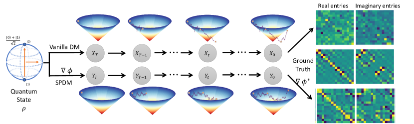
This article considers the generative modeling of the states of quantum systems, and an approach based on denoising diffusion model is proposed. The key contribution is an algorithmic innovation that respects the physical nature of quantum states. More precisely, the commonly used density matrix representation of mixed-state has to be complex-valued Hermitian, positive semi-definite, and trace one. Generic diffusion models, or other generative methods, may not be able to generate data that strictly satisfy these structural constraints, even if all training data do. To develop a machine learning algorithm that has physics hard-wired in, we leverage the recent development of Mirror Diffusion Model and design a previously-unconsidered mirror map, to enable strict structure-preserving generation. Both unconditional generation and conditional generation via classifier-free guidance are experimentally demonstrated efficacious, the latter even enabling the design of new quantum states when generated on unseen labels.
1 Introduction
Generative modeling, a specialized subfield of machine learning, is dedicated to creating models capable of generating new data points that closely match the statistical distribution of a given dataset. These models adeptly capture and replicate the patterns, structures, and characteristics of the input data, allowing them to yield new instances that seem to originate from the same distribution. Among them, diffusion model (Sohl-Dickstein et al., 2015; Ho et al., 2020; Song et al., 2021) has risen to prominence for its remarkable ability to produce high-quality data, especially notable in image generation (Rombach et al., 2022; Ho et al., 2022). The fundamental mechanism of diffusion model starts with adding noise to the data and progressively altering it into a tractable Gaussian prior with analytically available transition kernels. The model then effectively reverses this noise addition, reconstructing the data from its noised state through the application of learned score functions (Anderson, 1982; Haussmann & Pardoux, 1986). This process not only results in easily obtainable conditional score functions but also simplifies regression objectives, significantly boosting their capability in managing complex, high-dimensional data distributions.
Diffusion model has showcased impressive capabilities in generating various types of dataset across different application area, such as video synthesis (Ge et al., 2023; Blattmann et al., 2023), language modeling (Austin et al., 2021; Lou et al., 2023) and point cloud generation (Zeng et al., 2022; Luo & Hu, 2021). With the recent rise of AI4Science, the potential of diffusion model in tackling scientific problems also started being explored, including applications in biology (Jumper et al., 2021; Watson et al., 2022), chemistry (Duan et al., 2023; Hoogeboom et al., 2022), and climate science (Mardani et al., 2024). Other important notions relevant to this article include constrained generations (e.g., Liu et al., 2023; Fishman et al., 2023b, a; Lou & Ermon, 2023) and conditional generations (e.g., Dhariwal & Nichol, 2021; Ho & Salimans, 2022).
What is under-studied but important is the (classical) generative modeling of quantum data. This is not the same as quantum computing or quantum machine learning, because the goal is not to design quantum algorithms, but to develop algorithms that run on classical computers for handling quantum data. Similar to the already extremely successful application of the generation (and thus design) of molecular configurations (e.g., Watson et al., 2023; Duan et al., 2023), it would be useful to generate, for example, the states of quantum systems, before quantum computers become accessible to general researchers.
To be able to represent quantum states, which in general can be mixed states, one needs to be mindful of their structural constraints that originated from physics. For example, it is standard in quantum information and quantum computing to represent mixed states as complex-valued density matrices (Nielsen & Chuang, 2010), but such matrices have to be Hermitian, positive semidefinite, and trace one. Data-based generation of quantum density matrices therefore amounts to generative modeling in non-Euclidean spaces. Without strictly satisfying the structural constraints, the generated matrices will no longer correspond to quantum states (e.g., Huang et al., 2020). Unfortunately, generic generative modeling approaches will almost surely violate the constraints due to indispensable errors originated from finite data and compute. This article proposes the first machine learning methodology that generates density matrices similar to training data and strictly satisfying their structural constraints, based on hard-wiring these constraints into diffusion models via technique from convex optimization.
Imperative to mention is, machine learning has already been demonstrated promising for quantum problems, and it is rapidly becoming popular in the domain. There is even an interesting research frontier on quantum algorithms for generative modeling (e.g., Dallaire-Demers & Killoran, 2018; Khoshaman et al., 2018; Chakrabarti et al., 2019; Stein et al., 2021; Zhang et al., 2024; Chen & Zhao, 2024); however, this article still focuses on classical algorithm as quantum computer is not yet widely available, and existing results did not generate mixed states larger than 3-qubits. Meanwhile, classical algorithms have already been considered for many important quantum problems, such as the classification and regression of quantum states (e.g., Huang et al., 2020, 2022) and quantum state tomography (e.g., Torlai et al., 2018; Torlai & Melko, 2018; Carrasquilla et al., 2019; Vicentini et al., 2022; Jayakumar et al., 2023). The latter, roughly speaking, corresponds to the process of estimating one latent quantum density matrix through repeated, but necessarily noisy measurements of many copies of the same state. It is very important to clarify the similarity and difference between this work and quantum state tomography:
In fact, some may feel that quantum state tomography is already generative modeling, in a broad sense, because once the latent deterministic density matrix is recovered from noisy measurements, one can produce additional, synthetic classical measurements, which are random and ideally identically distributed with the training data. However, it is actually very different from the generative modeling of quantum states considered here, which might be in a narrow sense, however being a common setup in (classical) machine learning. More precisely, what this article considers is a collection of many different quantum mixed states, instead of classical observations of a single quantum state, and the goal is to generate more mixed states that are similar to the given ones. The problem of using machine learning to infer a single quantum state from classical observational data, i.e. state tomography, has already been considered by a series of seminal work mentioned above; there the probability distribution of data is uniquely determined by a latent quantum state, and thus one essentially needs to learn a -dimensional vector (if the latent state is an -qubit mixed state represented by a density matrix, then ). The new task of state generative modeling in this article, on the other hand, assumes mixed states are already given and they follow some unknown latent probability distribution, which can be represented by a probability density function of variables, and the goal is in some sense to learn this function, which is exponentially more complex than a -dimensional vector. An additional difference between this work and existing milestones on generative modeling for state tomography, from a machine learning methodology point of view, is that this work is based on denoising diffusion for generative modeling, while work cited above used, e.g., EBM, RBM, RNN instead.
What is the point of generating more quantum states?
One perspective is to actually create innovative states. Unconditional generation will simply produce states similar to those in the training data, but modern (diffusion) generative modeling technique also unleashes the ability of conditional generation. More precisely, given training data that carry different labels (e.g., traditionally labels could be ‘astronaut’, ‘horse’, etc., but in our case they can be ‘insulating’, ‘magnetic’, ‘topological’, etc.), we can not only generate under a label that already has training data (e.g., ‘astronaut’, or ‘magnetic’), but also generate under a label that has no training data (e.g., the famous ‘horse-riding astronaut’ (Heaven, 2022), or, this time, a motivating perspective of creating ‘topological magnetic’ states). This article humbly starts a first step toward this goal of scientific innovation, essentially via the interpolation/extrapolation of quantum data. The inter-/extra-polation, however, is in the sense of probability distributions but not sample points, because when one tries to design new states, it may not make sense to take, e.g., a specific ‘topological’ state and a specific ‘magnetic’ state and force a new ‘topological magnetic’ state based on them two alone. Instead, our conditional generative modeling approach hybrids multiple probability distributions and innovate just like prevailing generative AI tools.
Another application is, generative modeling can also estimate the probability distribution of states in the data, hence providing further quantitative insights for probing the physical process behind it. Some consideration of this aspect was already included in the state tomography literature (e.g., Carrasquilla et al., 2019), but not for an ensemble of states. Moreover, diffusion model excels in this regard. As a more recent generative approach, it is posited to be particularly effective for estimating density near the data manifold, even when data is high-dimensional but sample size is small, as long as there is a low-dimensional structure in the data. This is oftentimes the case for image and video generations, and their empirical successes were the root of this belief. Quantum density matrices data could be similar; at least, they are high-dimensional since dimension grows exponentially with the number of qubits, but scarce due to the cost of experiments. This is a case where diffusion generative model could be advantageous over traditional approaches.
In addition, generative model can serve as a sampler for crafting synthetic data that are experimentally expensive to harvest. Synthetic data that are statistically similar to training data are useful for discovering system properties through helping estimate observable values. The seminal work (Carrasquilla et al., 2019) showcases one such application for state-tomography type generative modeling. The idea is, generative modeling could help obtain more virtual ‘measurements’ from physical ones, hence improving the accuracy of the estimated latent state. Analogously, generative modeling of a distribution of mixed states can help the investigation of stochastic quantum systems, such as Random Transverse-field Ising Models (RTFIM) (Fisher, 1992, 1995; Kovács, 2022) and measurement-altered quantum critical systems (Murciano et al., 2023). The generated states can empower more accurate estimation of random parameters in the system, such as coupling and transverse field strengths.
2 Background
2.1 Unconditional Generation via Diffusion Model
Denoising diffusion generative models in Euclidean space admit many descriptions, with focuses on different perspectives, and here we adopt the stochastic differential equations (SDE) description (Song et al., 2021). Given samples of -valued random variable that follows the data distribution , denoising diffusion adopts a forward noising process followed by a backward denoising generation process to generate more samples of .
The forward process transports the (unknown latent) data distribution to a known, easy-to-sample distribution by evolving the initial condition via an SDE,
| (1) |
The evolution of the distribution’s density , given by , can be characterized by a partial differential equation (PDE) known as the Fokker-Planck Equation (FPE),
Upon certain choices of the drift and diffusion coefficient , the solution to the FPE will approach some limiting distribution. For example, corresponds to the well-known Variance-Preserving (VP) scheme, also known as Ornstein–Uhlenbeck process. In this case, will be a standard Gaussian .
The backward process then utilizes the time-reversal of the SDE (1) (Anderson, 1982). More precisely, if one considers
| (2) |
with , where , known as the score function, is given by
then we have , i.e. in distribution. In particular, the -time evolution of (2.1), , will follow the data distribution .
In practice, one considers evolving the forward dynamics for finite but large time , so that , and then initialize the backward dynamics using and simulate it numerically till to obtain approximate samples of the data distribution. Critically, the score function needs to be estimated in the forward process.
2.2 Diffusion Guidance for Conditional Generation
For the task of conditional generation, we have an additional input which is often a class label (e.g., a text sequence), and the goal is to sample from the conditional distribution given training data . For diffusion model, this means that we need the conditional score function . After applying Bayes’ rule, it’s clear that we can decompose the conditional score into two parts,
where is the usual score function of the data distribution, and is the gradient of the conditional probability of the addition input being . can be learned by training a diffusion model on unconditional data, and we need an estimator of to generate samples from the conditional distribution . Noticed that can be approximated by training a discriminative model such as a classifier based on the data-label pair . In practice, practitioners often use pre-tained classifier models to estimate .
Dhariwal & Nichol (2021) exploited this fact and proposed the technique of classifier-based diffusion guidance, originally for boosting the sample quality generated by diffusion models. Instead of , they proposed to sample from a condition-enhanced distribution,
The score of this condition-enhanced distribution can be computed by
is called the strength of the guidance, which amplifies the influence of the conditioning when setting to a scale larger than . When , the distribution is sharpened and focused onto its mode that corresponds to the condition (Dieleman, 2022). By tuning , classifier guidance allows us to capture the influence of the condition signal.
However, classifier-based diffusion guidance can become impractical due to the expensive cost of training a separate classifier model. Such a classifier often requires to be noise-robust to handle the noise-corrupted input during the sampling process. Ho & Salimans (2022) proposed classifier-free diffusion guidance to sample from the condition-enhanced distribution without the need for an extra discriminative model. Their insight came from another writing of Bayes’ rule: can also be decomposed as,
Therefore, classifier-free diffusion guidance motivates the training of a model that functions both as the conditional score and the unconditional score , depending on whether an additional condition input is given. We will use classifier-free guidance due to improved performance and computational cost.
2.3 Density Matrix Representation of Quantum State
Since we will consider the unconditional and conditional generations of quantum states, let’s review some of their basics. A quantum state describes the physical status of a quantum system. For generality and with some motivations being quantum computing and quantum information in mind, we consider mixed states, which can be represented by density matrices (in theory, they are operators, but once we fix the bases of the Hilbert space, they become finite dimensional objects).
Precisely, a (quantum) density matrix is a matrix with each element being a complex number, which satisfies the following structural constraints (e.g., Nielsen & Chuang, 2010):
It is Hermitian, with trace 1, and positive semi-definite.
Notations: Here we denote the set of complex Hermitian matrices of dimension as ,
| (3) |
where is the conjugate transpose of , defined through . We also denoted the set of positive definite complex Hermitian matrices of dimension as
| (4) |
Definition 2.1.
A qubit quantum state is an element of with trace 1.
Because of the structural constraints, the generative modeling of quantum states is nontrivial but an interesting machine-learning problem. Ideally speaking, if there were an infinite amount of data and infinite computational resources (so that generative modeling can be exact), the training data already implicitly carry information about the structural constraints, and then the generated data will also respect the constraints, thus yielding true quantum states. Nevertheless, in practice the generation is plagued with various sources of error (e.g., statistical error of finite samples, (score) function approximation error, finite-time approximation of , numerical integration of the backward process, etc.) and generic generative modeling approaches that are not built to respect those constraints will likely generate samples that violate them, and the samples will no longer possess physical meaning and are hence useless. Therefore, in the following, we hardwire these important physical knowledge into our generative model, so that the constraints will be exactly satisfied.
3 Method
Our task is to generate new samples of quantum mixed states, from a distribution characterized by the training data. Out of the three structure constraints of density matrix representation of quantum states, Hermitianity is easy to handle as one can just work with the upper triangular part of the matrix. Trace one condition will only be minimally violated due to generation error, and we simply normalize the generated result by dividing its trace to strictly enforce this constraint. The most nontrivial constraint is the positive semi-definiteness. Since this is a convex constraint, we can leverage the recent approach of Mirror Diffusion Model (MDM) (Liu et al., 2023), which is a class of diffusion models that generate data on convex-constrained sets, to enable exact generation on . To achieve this goal, we work out a complex and multivariate extension of the results in MDM.
3.1 Mirror Map with Real Numbers
More precisely, the approach of MDM relies on a tool from convex optimization known as mirror map. It can create a nonlinear bijection that maps the data from the constrained primal space to an unconstrained dual space, which is Euclidean. This bijection serves as a coordinate transformation, i.e. a pair of exact encoder and decoder. A mirror map is defined as follows:
Definition 3.1.
Given a convex constrained set, , is called mirror map if is a twice differentiable function that is strictly convex and satisfying:
is an invertible map from the constrained primal space to an unconstrained dual space , which is also called the mirror space.
Its inverse enjoys a pleasant characterization from convex analysis (Rockafellar, 2015). Namely, by defining the dual function of as the inverse (as a mapping) of is the same as the gradient of , i.e.
Therefore, acts as a pair of encoder-decoder that transform each datum between the primal constrained space and the unconstrained mirror space .
3.2 Mirror Map for Complex-Valued Density Matrices
A complication is that our data consists of complex-valued matrices, different from real vectors and matrices typically considered in convex optimization. Therefore, what remains to be described is the construction of a strictly convex potential for the class of positive definite Hermitian matrices. It turns out that the negative von Neumann entropy satisfies the need.
The von Neumann entropy (e.g., Bengtsson & Życzkowski, 2017) is an extension of the concept of Shannon entropy to quantum states. For , the negative von Neumann entropy is defined as,
| (5) |
The mirror map and its inverse are computed analytically as
| (6) |
where log and exp are matrix logarithm and matrix exponential. Specifically, we define the matrix logarithm to be if admits spectral decomposition , where are positive real numbers, are a set of complex-valued vectors that are also orthonormal basis of
Proposition 3.2.
given by (6) is a pair of bijective mappings between the set of positive definite complex Hermitian matrices and the set of complex Hermitian matrices . Moreover, is the inverse of .
Proof. Please see Appendix.A.2.
3.3 Generative Modeling in Primal Space Based on Diffusion in Dual Space
The gradient map of negative von Neumann entropy, , allows us to transform the problem of learning and sampling the data distribution over , to that for a new distribution over the mirror space , where is the push-forward operation. Moreover, although is still a convex-constrained set due to each element being a Hermitian matrix, enjoys a much simpler structure due to the fact that , i.e. it is isomorphic to an unconstrained real Euclidean space of dimension . This is because each complex Hermitian matrix can be represented using only its upper or lower triangular entries. Since complex Hermitian has real diagonal values, the diagonal contributes dimension. There are strict upper triangular entries, each having a complex value. Each complex entry can be represented with a point in . Therefore, the total dimension is and linearity guarantees the isomorphism.
Since diffusion models leverage a neural network parameterization of the score function, and most neural networks have not been designed for complex numbers, we utilize the isomorphism mentioned above and further transform into a vector in . This enables us to represent the score function based on simple Euclidean space again.
3.4 Summary of Methodology
Our approach can be summarized in the following steps. We take quantum state data in and apply the mirror map to transform them into . We extract the upper triangular entries and create their real representation as a vector in the dual space . On the dual space, we build a diffusion model that transforms the distribution to a Gaussian measure. We train the score neural network with a score-matching loss on the dual space.
For quantum state generation, we simulate the reverse-time SDE or marginally equivalent probability flow ODE with the learned score network to generate new samples , which is on . We compute its representation as a complex Hermitian matrices through , where stands for the isomorphic transformation between the two spaces. We generate a new quantum state by applying the inverse of mirror map, , which approximately satisfies the desired data distribution .
4 Experiments
As this work is the first on the generative modeling of quantum data, there is no existing approach to compare to, although both statistical and physical means for assessing the success still exist. Moreover, no public dataset has been curated either, and we will therefore prove the concept using physical but synthetic data.
More precisely, we will consider three labeled classes of data, corresponding to quantum mixed states of a qubit system with three different levels of entanglements. We will first conduct unconditional generation, from the distribution of the union of all classes. Then we will perform conditional generation, from the same union distribution but conditioned on the class label; results similar to that of individually generating from each class would be seen. Finally, we will investigate conditional generation beyond the known class labels, i.e., the ability to interpolate/extrapolate across existing classes in the training data.
4.1 Problem Setup
To demonstrate the efficacy of our method, we consider an example of generating quantum states based on training data consisting of quantum states with three different levels of entanglement between qubits.
Product state. Let be quantum states of one qubit. The product state with no entanglement for a qubit system is given by
| (7) |
To simplify the setting, we consider to be sampled i.i.d. from the same distribution over quantum states of one qubit. Product state is a quantum state of the system that corresponds to the situation where there is no quantum entanglement between any of the two qubits, i.e., each qubit has a quantum state that can be independently described regardless of others.
Pairwisely entangled state. We now entangle qubits to create entangled state from product state . Let be complex-valued unitary matrices of dimension , where corresponds to the quantum entanglement between qubit and , corresponds to the quantum entanglement between qubit and . A pairwisely entangled state for the qubit system is given by
| (8) |
Such states correspond to a situation where there is simultaneous quantum entanglement between qubits and , as well as qubits and , but no entanglement between any other qubit pair. Since and refer to entanglement between only two qubits, the two unitary matrices are created with complex unitary matrices of dimension .
In this experiment, we let be unitary matrices of dimension , sampled from the Haar measure of . Haar measure generalizes the concept of uniform distribution to compact Lie groups. are then created from in the following way:
where is the identity matrix.
Fully entangled state. We now entangle more qubits to create further entangled state from product state . For , let be complex unitary matrices of dimension , where corresponds to the quantum entanglement between qubit and . Consider a fully entangled state for the qubit system given by
| (9) |
Fully entangled state is a quantum state of the system that corresponds to a situation where there is simultaneous entanglement between any pair of qubits. Each matrix corresponds to the entanglement between only two qubits, thus the matrix is created using complex unitary matrices of dimension .
are created from in the following way:
where permutes the rows and columns that correspond to qubit and , is the identity matrix.
4.2 Data Preparation
This section describes how we generate thethree classes of quantum states, which altogether constitute our training set.
Single qubit quantum state distribution. In the generation process of product state, we consider the scenario where each qubit has a quantum state sampled i.i.d. from the same distribution , which is defined by the following procedure. Let , where , with . is computed as
| (10) |
We consider to be the distribution of generated via eq.(10). By construction, is a positive definite Hermitian matrix with trace , thus a valid quantum state.
| Class | ||||||
|---|---|---|---|---|---|---|
| Unconditional | Mixture | 0.020 | 0.000076 | 0.0000110 | ||
| Product | 0.00079 | 0.011 | 0.000070 | 0.0000025 | ||
| Conditional | Pairwisely | 0.00100 | 0.018 | 0.000082 | 0.0000061 | |
| Fully | 0.00092 | 0.026 | 0.000100 | 0.0000062 | ||
| Magnitude reference | – | 0.0854 | 0.1554 | 1.7484 | 1.1236 | 0.0134 |
Haar measure of . To generate the training data for pairwisely entangled and fully entangled states, we chose to sample from the Haar measure on to create unbiased quantum entanglement matrices between qubit and . is the set of matrices defined as,
Sampling a probability distribution on , such as the Haar measure, is also an interesting task. One may view it as a sampling problem on a constrained set, but note is actually a non-convex constrained set, and thus common constrained sampling tools (e.g., projected Langevin (Bubeck et al., 2015), sophisticated MCMC walkers (Lovász & Simonovits, 1993; Lovász, 1999; Kannan & Narayanan, 2009; Chen et al., 2018), mirror Langevin (Zhang et al., 2020; Li et al., 2022)) may not suit well. Fortunately, due to the Lie group structure of , the problem can be solved by considering the dynamics,
| (11) |
where , is an element in the Lie algebra, is the Brownian motion over the vector space . The Lie algebra and Brownian motion is defined as,
where , are independent one dimensional Brownian motion. One notable property of the diffusion process described in (11) is that it converges to a unique invariant distribution and the -marginal of its invariant distribution is the Haar measure of (Kong & Tao, 2024). Therefore, by numerically integrating (11), we can approximately sample uniformly from the unitary group to generate the quantum entanglement matrices. This numerical integration can be done computational-efficiently with exactly remaining on via the operator splitting approach (Tao & Ohsawa, 2020).
4.3 Evaluation
In this section, we discuss the metrics and observables (since the data distribution is high dimensional) used for evaluating the sample quality of the generated quantum states. Both statistical and physical quantities will be used.
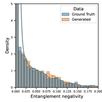
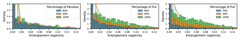
Entanglement negativity. Entanglement negativity is a non-negative measure of the amount of quantum entanglement present in a quantum state. Entanglement negativity is an entanglement monotone whose value does not increase under local operations and classical communication. Consider a composite quantum system consisting of two subsystems and , described by a density matrix in a Hilbert space that is the tensor product of the spaces of and . We denote the transpose operator on the space of subsystem A as . We denote the partial transpose of with respect to subsystem as , which can be computed as . Then, the entanglement negativity is defined as,
where are eigenvalues of . A high value of represents a high level of quantum entanglement.
Distributional-wise metric. To evaluate the similarity between high-dim probability distributions, we mainly use Sliced Wasserstein Distance (SWD) (Kolouri et al., 2019), Maximum Sliced Wasserstein Distance (MSWD) (Deshpande et al., 2019), and Maximum Mean Discrepancies (MMD) (Gretton et al., 2012), in addition to the standard Wasserstein distance, as they suffer less from the curse of dimensionality. Within the family of MMDs, we consider Energy-MMD, which is computed with kernel . We also compute the 1-Wasserstein distance based on values of the physically meaningful low-dim observable of entanglement negativity.
4.4 Training
We train on a dataset of samples, distributed equally across all three classes of quantum states. The entire dataset is first transformed to the dual space by applying the mirror map. Then a DDPM is trained on the transformed dataset. We train for iterations with AdamW optimizer, using an initial learning rate of and decay rate of every AdamW steps. We summarize our neural network architecture in Appendix.A.3. We adopt the same data post-processing and metrics evaluation used in (Chen et al., 2023), and we elaborate them in Appendix.A.4.
4.5 Results
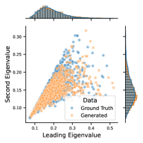
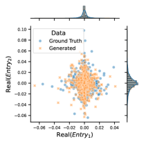
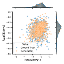
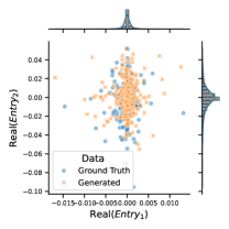
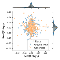
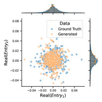
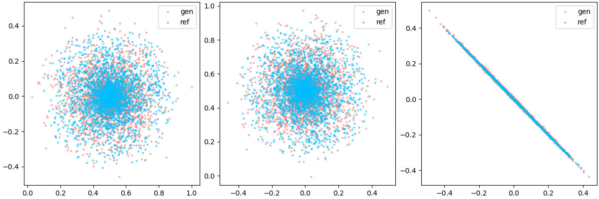
SPDM accurately learns the distribution of quantum states. Table 1 summarizes our quantitative results for both conditional and unconditional generation of three classes of quantum states. Figure 2 and Figure 3 depict the generated samples compared against ground truth. Our method manages to learn accurately the correct distribution of eigenvalues, which is extremely sensitive to all the entries in the matrix. We note that product states, pairwisely entangled states, and fully entangled states considered in this work share an identical distribution of eigenvalues since the spectrum of matrices is invariant under unitary conjugations. However, they have distinct marginal distributions for each entry due to the quantum entanglement. Our method successfully predicts the correct joint distribution of all the entries in the density matrix, which is also confirmed by small values in all distribution-based metrics listed in Table 1.
SPDM generates the correct level of quantum entanglement between qubits. Other than eigenvalues and distribution-based metrics, another assessment of generation quality is whether the generated samples demonstrate the same level of entanglement as the training data. We use entanglement negativity to capture the degree of quantum entanglement between two subsystems. As is evident from Table 1 and Figure 2, our method accurately generates samples with the same amount of quantum entanglement as the training data. This implies that under our framework, diffusion models manage to learn the sophisticated relationships between entangled entries and reproduce such entanglements in the generation process.
SPDM enables the design of physically-meaningful new quantum states. We generate new labels by taking a convex combination of the one-hot encodings of seen classes. Then we conditionally generate samples that correspond to these new labels with our model. Figure 4 demonstrated the quantum entanglement level of the resulting data. When generating under labels that are mixtures of two classes with different entanglements, the model produces data with an entanglement level in the middle ground of the two classes, which is in accordance with the interpolation ratio we used in generating new labels. This implies that our method manages to learn a meaningful embedding of class labels that also reflects the interpolation of entanglement level among quantum data. The model allows an extrapolation to unseen quantum states. This means that our model is capable of designing quantum states with specific (new) entanglement level controlled by a manually created label.
5 Conclusion
We developed the first diffusion-based method for the generative modeling of quantum states. Our method hard codes physical knowledge into the generative models and generates samples that strictly satisfy the structural constraints of quantum states. We demonstrate that the model accurately learns and reproduces the distribution of quantum states represented by high dimensional density matrix, and can even create physically-meaningful quantum states of unseen level of entanglements, via conditional generation. In the future, it will be an interesting task to design neural network architectures for parametrizing the score function that specialize in quantum state generation for even better generation quality.
6 Impact Statement
This paper presents work whose goal is to advance the field of machine learning and quantum sciences. There could be potential societal consequences of our work, none of which we feel must be specifically highlighted here.
References
- Anderson (1982) Anderson, B. D. Reverse-time diffusion equation models. Stochastic Processes and their Applications, 12(3):313–326, 1982.
- Austin et al. (2021) Austin, J., Johnson, D. D., Ho, J., Tarlow, D., and Van Den Berg, R. Structured denoising diffusion models in discrete state-spaces. Advances in Neural Information Processing Systems, 34:17981–17993, 2021.
- Bengtsson & Życzkowski (2017) Bengtsson, I. and Życzkowski, K. Geometry of quantum states: an introduction to quantum entanglement. Cambridge university press, 2017.
- Blattmann et al. (2023) Blattmann, A., Rombach, R., Ling, H., Dockhorn, T., Kim, S. W., Fidler, S., and Kreis, K. Align your latents: High-resolution video synthesis with latent diffusion models. In Proceedings of the IEEE/CVF Conference on Computer Vision and Pattern Recognition, pp. 22563–22575, 2023.
- Bubeck et al. (2015) Bubeck, S., Eldan, R., and Lehec, J. Finite-time analysis of projected langevin monte carlo. Advances in Neural Information Processing Systems, 28, 2015.
- Carrasquilla et al. (2019) Carrasquilla, J., Torlai, G., Melko, R. G., and Aolita, L. Reconstructing quantum states with generative models. Nature Machine Intelligence, 1(3):155–161, 2019.
- Chakrabarti et al. (2019) Chakrabarti, S., Yiming, H., Li, T., Feizi, S., and Wu, X. Quantum wasserstein generative adversarial networks. Advances in Neural Information Processing Systems, 32, 2019.
- Chen & Zhao (2024) Chen, C. and Zhao, Q. Quantum generative diffusion model. arXiv preprint arXiv:2401.07039, 2024.
- Chen et al. (2023) Chen, T., Liu, G.-H., Tao, M., and Theodorou, E. A. Deep momentum multi-marginal schr” odinger bridge. NeurIPS, 2023.
- Chen et al. (2018) Chen, Y., Dwivedi, R., Wainwright, M. J., and Yu, B. Fast mcmc sampling algorithms on polytopes. The Journal of Machine Learning Research, 19(1):2146–2231, 2018.
- Dallaire-Demers & Killoran (2018) Dallaire-Demers, P.-L. and Killoran, N. Quantum generative adversarial networks. Physical Review A, 98(1):012324, 2018.
- Deshpande et al. (2019) Deshpande, I., Hu, Y.-T., Sun, R., Pyrros, A., Siddiqui, N., Koyejo, S., Zhao, Z., Forsyth, D., and Schwing, A. G. Max-sliced wasserstein distance and its use for gans. In Proceedings of the IEEE/CVF Conference on Computer Vision and Pattern Recognition, pp. 10648–10656, 2019.
- Dhariwal & Nichol (2021) Dhariwal, P. and Nichol, A. Diffusion models beat gans on image synthesis. Advances in neural information processing systems, 34:8780–8794, 2021.
- Dieleman (2022) Dieleman, S. Guidance: a cheat code for diffusion models, 2022. URL https://benanne.github.io/2022/05/26/guidance.html.
- Duan et al. (2023) Duan, C., Du, Y., Jia, H., and Kulik, H. J. Accurate transition state generation with an object-aware equivariant elementary reaction diffusion model. Nature Computational Science, 2023.
- Fisher (1992) Fisher, D. S. Random transverse field ising spin chains. Physical review letters, 69(3):534, 1992.
- Fisher (1995) Fisher, D. S. Critical behavior of random transverse-field ising spin chains. Physical review b, 51(10):6411, 1995.
- Fishman et al. (2023a) Fishman, N., Klarner, L., De Bortoli, V., Mathieu, E., and Hutchinson, M. Diffusion models for constrained domains. TMLR, 2023a.
- Fishman et al. (2023b) Fishman, N., Klarner, L., Mathieu, E., Hutchinson, M., and De Bortoli, V. Metropolis sampling for constrained diffusion models. NeurIPS, 2023b.
- Ge et al. (2023) Ge, S., Nah, S., Liu, G., Poon, T., Tao, A., Catanzaro, B., Jacobs, D., Huang, J.-B., Liu, M.-Y., and Balaji, Y. Preserve your own correlation: A noise prior for video diffusion models. In Proceedings of the IEEE/CVF International Conference on Computer Vision, pp. 22930–22941, 2023.
- Gretton et al. (2012) Gretton, A., Borgwardt, K. M., Rasch, M. J., Schölkopf, B., and Smola, A. A kernel two-sample test. The Journal of Machine Learning Research, 13(1):723–773, 2012.
- Haussmann & Pardoux (1986) Haussmann, U. G. and Pardoux, E. Time reversal of diffusions. The Annals of Probability, pp. 1188–1205, 1986.
- Heaven (2022) Heaven, W. D. Horse riding astronaut, 2022. URL https://www.technologyreview.com/2022/04/06/1049061/dalle-openai-gpt3-ai-agi-multimodal-image-generation/.
- Ho & Salimans (2022) Ho, J. and Salimans, T. Classifier-free diffusion guidance. arXiv preprint arXiv:2207.12598, 2022.
- Ho et al. (2020) Ho, J., Jain, A., and Abbeel, P. Denoising diffusion probabilistic models. Advances in neural information processing systems, 33:6840–6851, 2020.
- Ho et al. (2022) Ho, J., Saharia, C., Chan, W., Fleet, D. J., Norouzi, M., and Salimans, T. Cascaded diffusion models for high fidelity image generation. The Journal of Machine Learning Research, 23(1):2249–2281, 2022.
- Hoogeboom et al. (2022) Hoogeboom, E., Satorras, V. G., Vignac, C., and Welling, M. Equivariant diffusion for molecule generation in 3d. In International conference on machine learning, pp. 8867–8887. PMLR, 2022.
- Huang et al. (2020) Huang, H.-Y., Kueng, R., and Preskill, J. Predicting many properties of a quantum system from very few measurements. Nature Physics, 16(10):1050–1057, 2020.
- Huang et al. (2022) Huang, H.-Y., Kueng, R., Torlai, G., Albert, V. V., and Preskill, J. Provably efficient machine learning for quantum many-body problems. Science, 377(6613):eabk3333, 2022.
- Jayakumar et al. (2023) Jayakumar, A., Vuffray, M., and Lokhov, A. Y. Learning energy-based representations of quantum many-body states. arXiv preprint arXiv:2304.04058, 2023.
- Jumper et al. (2021) Jumper, J., Evans, R., Pritzel, A., Green, T., Figurnov, M., Ronneberger, O., Tunyasuvunakool, K., Bates, R., Žídek, A., Potapenko, A., et al. Highly accurate protein structure prediction with alphafold. Nature, 596(7873):583–589, 2021.
- Kannan & Narayanan (2009) Kannan, R. and Narayanan, H. Random walks on polytopes and an affine interior point method for linear programming. In Proceedings of the forty-first annual ACM symposium on Theory of computing, pp. 561–570, 2009.
- Khoshaman et al. (2018) Khoshaman, A., Vinci, W., Denis, B., Andriyash, E., Sadeghi, H., and Amin, M. H. Quantum variational autoencoder. Quantum Science and Technology, 4(1):014001, 2018.
- Kolouri et al. (2019) Kolouri, S., Nadjahi, K., Simsekli, U., Badeau, R., and Rohde, G. Generalized sliced wasserstein distances. Advances in neural information processing systems, 32, 2019.
- Kong & Tao (2024) Kong, L. and Tao, M. Convergence of kinetic langevin monte carlo on lie groups. arXiv:2403.12012, 2024.
- Kovács (2022) Kovács, I. A. Quantum multicritical point in the two-and three-dimensional random transverse-field ising model. Physical Review Research, 4(1):013072, 2022.
- Li et al. (2022) Li, R., Tao, M., Vempala, S. S., and Wibisono, A. The mirror langevin algorithm converges with vanishing bias. In International Conference on Algorithmic Learning Theory, pp. 718–742. PMLR, 2022.
- Liu et al. (2023) Liu, G.-H., Chen, T., Theodorou, E. A., and Tao, M. Mirror diffusion models for constrained and watermarked generation. NeurIPS, 2023.
- Lou & Ermon (2023) Lou, A. and Ermon, S. Reflected diffusion models. ICML, 2023.
- Lou et al. (2023) Lou, A., Meng, C., and Ermon, S. Discrete diffusion language modeling by estimating the ratios of the data distribution. NeurIPS, 2023.
- Lovász (1999) Lovász, L. Hit-and-run mixes fast. Mathematical programming, 86:443–461, 1999.
- Lovász & Simonovits (1993) Lovász, L. and Simonovits, M. Random walks in a convex body and an improved volume algorithm. Random structures & algorithms, 4(4):359–412, 1993.
- Luo & Hu (2021) Luo, S. and Hu, W. Diffusion probabilistic models for 3d point cloud generation. In Proceedings of the IEEE/CVF Conference on Computer Vision and Pattern Recognition, pp. 2837–2845, 2021.
- Mardani et al. (2024) Mardani, M., Brenowitz, N., Cohen, Y., Pathak, J., Chen, C.-Y., Liu, C.-C., Vahdat, A., Kashinath, K., Kautz, J., and Pritchard, M. Residual diffusion modeling for km-scale atmospheric downscaling. 2024.
- Murciano et al. (2023) Murciano, S., Sala, P., Liu, Y., Mong, R. S., and Alicea, J. Measurement-altered ising quantum criticality. Physical Review X, 13(4):041042, 2023.
- Nielsen & Chuang (2010) Nielsen, M. A. and Chuang, I. L. Quantum computation and quantum information. Cambridge university press, 2010.
- Rockafellar (2015) Rockafellar, R. Convex analysis. Princeton landmarks in mathematics and physics. Princeton University Press, 2015.
- Rombach et al. (2022) Rombach, R., Blattmann, A., Lorenz, D., Esser, P., and Ommer, B. High-resolution image synthesis with latent diffusion models. In Proceedings of the IEEE/CVF conference on computer vision and pattern recognition, pp. 10684–10695, 2022.
- Sohl-Dickstein et al. (2015) Sohl-Dickstein, J., Weiss, E., Maheswaranathan, N., and Ganguli, S. Deep unsupervised learning using nonequilibrium thermodynamics. ICML, 2015.
- Song et al. (2021) Song, Y., Sohl-Dickstein, J., Kingma, D. P., Kumar, A., Ermon, S., and Poole, B. Score-based generative modeling through stochastic differential equations. ICLR, 2021.
- Stein et al. (2021) Stein, S. A., Baheri, B., Chen, D., Mao, Y., Guan, Q., Li, A., Fang, B., and Xu, S. Qugan: A quantum state fidelity based generative adversarial network. In 2021 IEEE International Conference on Quantum Computing and Engineering (QCE), pp. 71–81. IEEE, 2021.
- Tao & Ohsawa (2020) Tao, M. and Ohsawa, T. Variational optimization on lie groups, with examples of leading (generalized) eigenvalue problems. In International Conference on Artificial Intelligence and Statistics, pp. 4269–4280. PMLR, 2020.
- Torlai & Melko (2018) Torlai, G. and Melko, R. G. Latent space purification via neural density operators. Physical review letters, 120(24):240503, 2018.
- Torlai et al. (2018) Torlai, G., Mazzola, G., Carrasquilla, J., Troyer, M., Melko, R., and Carleo, G. Neural-network quantum state tomography. Nature Physics, 14(5):447–450, 2018.
- Vicentini et al. (2022) Vicentini, F., Rossi, R., and Carleo, G. Positive-definite parametrization of mixed quantum states with deep neural networks. arXiv preprint arXiv:2206.13488, 2022.
- Vincent (2011) Vincent, P. A connection between score matching and denoising autoencoders. Neural computation, 23(7):1661–1674, 2011.
- Watson et al. (2022) Watson, J. L., Juergens, D., Bennett, N. R., Trippe, B. L., Yim, J., Eisenach, H. E., Ahern, W., Borst, A. J., Ragotte, R. J., Milles, L. F., et al. Broadly applicable and accurate protein design by integrating structure prediction networks and diffusion generative models. BioRxiv, pp. 2022–12, 2022.
- Watson et al. (2023) Watson, J. L. et al. De novo design of protein structure and function with rfdiffusion. Nature, 2023.
- Zeng et al. (2022) Zeng, X., Vahdat, A., Williams, F., Gojcic, Z., Litany, O., Fidler, S., and Kreis, K. Lion: Latent point diffusion models for 3d shape generation. arXiv preprint arXiv:2210.06978, 2022.
- Zhang et al. (2024) Zhang, B., Xu, P., Chen, X., and Zhuang, Q. Generative quantum machine learning via denoising diffusion probabilistic models. Physical Review Letters, 132(10):100602, 2024.
- Zhang et al. (2020) Zhang, K. S., Peyré, G., Fadili, J., and Pereyra, M. Wasserstein control of mirror langevin monte carlo. In Conference on Learning Theory, pp. 3814–3841. PMLR, 2020.
Appendix A Appendix
A.1 Vanilla SGM on Quantum State Dataset
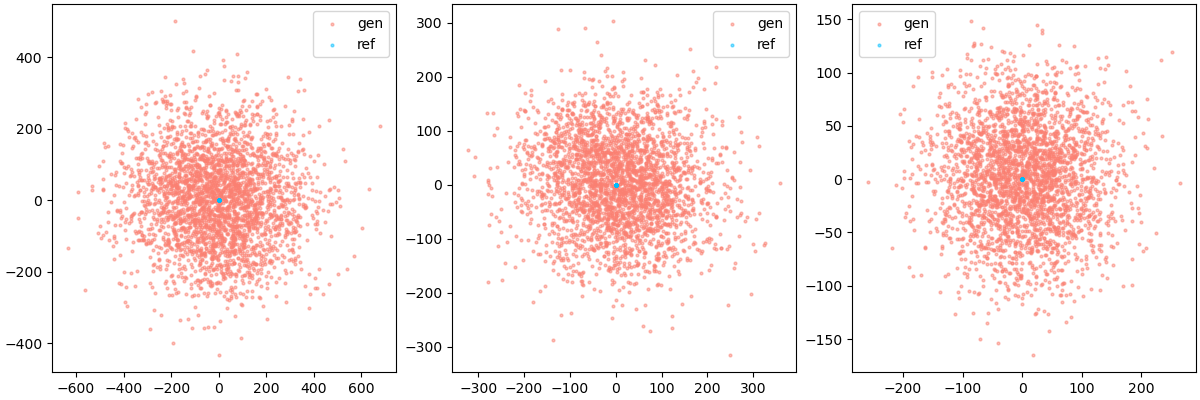
In our research, we demonstrate that conventional score-based generative models (SGMs) fall short in reliably generating high-dimensional quantum datasets. Figure 5 exemplifies that, although these SGMs can precisely mimic the distribution of a 1-qubit quantum state (4 dimensions), they face significant challenges due to the curse of dimensionality when the dimensionality is expanded to a 4-qubit state (256 dimensions), as highlighted in Figure 6. This limitation likely stems from the current neural network parameterization strategies. Identifying an efficient network architecture capable of effectively capturing the essence of quantum states remains a pivotal, yet unresolved, question, which we aim to address in future work.
A.2 Proof of Proposition.3.2
Proof.
We first show that is a mapping from to and is a mapping from to . For any , , we denote their spectral decomposition as , with complex-valued eigenvectors and form orthonormal basis of , and eigenvalues , ,
This implies that is a complex Hermitian matrix for any . Similarly,
Since has positive eigenvalues , for any .
Now we need to show that and are inverse of each other.
This implies that is the identity map on .
Similarly, is the identity map on . Therefore, we conclude that is a pair of bijective mappings that are inverse of each other. ∎
A.3 Training and neural network
Our neural network takes an input pair , where is the spatial input, is the time, and is the condition. Time is passed through a module to generate a standard sinusoidal embedding and then fed to fully connected layers with Sigmoid Linear Unit (SiLU) and generate an output . Spatial input is passed through an MLP with residual blocks, each containing linear layers with hidden dimension and SiLU activation. This generates an output . The condition , considered to be a one-hot encoding in our case, is fed to fully connected layers with SiLU and generates an output . Our final output out is computed through,
where Outmod is an out module that consists of fully connected layers with hidden dimension and SiLU activation, stands for group normalization.
A.4 Evaluation
The 1-Wasserstein Distance suffers from the curse of dimensionality seriously which is pointed out in Appendix.C in (Chen et al., 2023). Therefore, we use various metrics to comprehensively evaluate the distance between high dimensional distributions. For the scalar distribution of negativity, we stick to using 1-Wasserstein distance. In the main results, when evaluating the sample quality of generated quantum states (which is a density of dimensions), we use the Sliced-Wasserstein Distance (SWD) type and Maximum Mean Discrepancies (MMD) type of metrics as our major criterion. These metrics include Energy Maximum Mean Discrepancy (Energy-MMD), Max-sliced Wasserstein distance (MSWD), and Sliced-Wasserstein Distance (SWD). Here, Energy-MMD is the MMD distance computed with kernel . Our implementation is adapted from Geoloss (, Energy-MMD) and POT (SWD, MSWD).