Tests of the Kerr Hypothesis with MAXI J1803-298 Using Different RELXILL_NK Flavors

Abstract

Iron line spectroscopy has been one of the leading methods not only for measuring the spins of accreting black holes but also for testing fundamental physics. Basing on such a method, we present an analysis of a dataset observed simultaneously by NuSTAR and NICER for the black hole binary candidate MAXI J1803-298, which shows prominent relativistic reflection features. Various relxill_nk flavors are utilized to test the Kerr black hole hypothesis. The results obtained from our analysis provide stringent constraints on Johannsen deformation parameter $\alpha_{13}$ with the highest precise to date, namely $\alpha_{13}=0.023^{+0.071}_{-0.038}$ from relxillD_nk and $\alpha_{13}=0.006^{+0.045}_{-0.022}$ from relxillion_nk respectively in 3-$\sigma$ credible lever, where Johannsen metric reduces to Kerr metric when $\alpha_{13}$ vanishes. Furthermore, we investigate the best model-fit results using Akaike Information Criterion and assess its systematic uncertainties.

1 Introduction

Since Einstein proposed General Relativity in late 1915, it has found applications across various physical phenomena and has undergone numerous tests in the weak field regime (will2014confrontation). Over the decades, advancements in instruments and technology have made the testing of general relativity in strong gravitational regimes a prominent and contemporary research focus. Astrophysical black holes, which can be described by the Kerr solution (kerr1963gravitational; carter1971axisymmetric; robinson1975uniqueness), serve as an ideal laboratory for probing strong gravity.

The presence of an accretion disk, nearby stars, or a potential non-vanishing electric charge of the black hole is typically negligible in the strong gravitational field near the event horizon (bambi2009black; bambi2018astrophysical; cardoso2019testing). Conversely, certain plausible macroscopic deviations from the Kerr metric arise in the presence of quantum gravity effects (dvali2013black; giddings2017astronomical; giddings2018event), exotic matter (giddings2018event; herdeiro2016kerr), and various modified theories of gravity (kleihaus2011rotating; ayzenberg2014slowly; sotiriou2014black). Consequently, testing the Kerr metric proves to be an effective approach for exploring the strong gravitational field regime.

Numerous methods for testing the Kerr hypothesis have been explored, primarily encompassing electromagnetic techniques (johannsen2016sgr; Bambi:2016sac) and, in recent years, gravitational wave approaches (glampedakis2006mapping; yunes2013gravitational; scientific2016tests; yunes2016theoretical). The X-ray reflection spectrum is generally used to study the relativistic effects on the inner part of the accretion disk around BHs and to understand the properties of spacetime (bambi2021towards). There are many observational constraints already published using X-ray reflection spectrum originated from the accretion disk around Black Holes to test the Kerr hypothesis (cao2018testing; xu2018study; tripathi2019constraints; tripathi2019toward; tripathi2019constraining; abdikamalov2019testing). Among these approaches, the disk-corona model is regarded as a phenomenological model describing the relationship between the accretion disk and the ionized corona in a black hole system.

The thermal photons emitted from the disk undergo inverse Compton scattering within the corona, characterized by high temperatures (approximately 100 keV), and some of them are reflected to the disk, which is the so-called reflection spectrum. The most prominent features of the reflection spectrum are often characterized by the iron $K\alpha$ line around 6.4 keV, depending on the ionization of iron atoms, and the Compton hump peaked around 20–30 keV. In the rest frame of the gas, fluorescent emission lines display narrow profiles; however, in a strong gravity region, the $K\alpha$ line undergoes broadening due to relativistic effects, which indicates that it is one of the most potential tools that can be used to test relativistic effects in strong gravity region (cao2018testing; abdikamalov2019testing; tripathi2020testing).

The relxill_nk model(bambi2017testing; abdikamalov2019public), an extension of the relxill package(dauser2013irradiation; garcia2014improved), is a versatile tool for analyzing the reflection features of a geometrically thin and optically thick disk in non-Kerr spacetimes. The model employs a parametric black hole spacetime metric, where a set of deformation parameters parameterizes deviations from the Kerr solution. The Kerr metric is recovered when all the deformation parameters vanish (cao2018testing; abdikamalov2019testing; tripathi2020testing).

This paper details the spectral analysis conducted on the observational data during the outburst of the Galactic black hole binary candidate MAXI J1803-298. The outburst of this black hole binary candidate was first captured by the Gas Slit Camera of the Monitor of All-sky X-ray Image (MAXI/GSC) nova alert system at 19:50 UT on May 1st, 2021, located at R.A.=$270.923^{\circ}$, Dec=$-29.804^{\circ}$ (J2000) (serino2021maxi). A comprehensive multiwavelength follow-up of the discovery outburst and the timing analysis of the black hole candidate MAXI J1803$-$298 is presented in sanchez2022hard and zhu2023timing. These findings indicate a state transition from the low/hard state to the hard intermediate state, followed by the soft intermediate state, and ultimately reaching the high/soft state. The works of feng2022spin and coughenour2023reflection previously examined variability and reflection features, revealing a notable relativistically broadened iron line component in the spectrum with an extraordinarily high value of spin parameter.

Based on the reflection feature from MAXI J1803-298 within a soft intermediate state, we mainly test the Kerr metric with different flavors of model relxill_nk and then discuss the impact of different relxill_nk flavors in fitting data from NuSTAR and NICER in this work. Stringent constraints on its parameters have been obtained, and these findings reveal no significant distinctions among different flavors of relxill_nk. Subsequently, the Akaike Information Criterion (AIC) was employed to assess the congruence among diverse models for the purpose of selecting the best-fitting model.

The contents of this paper are organized as follows. In Section 2, we present the observations of MAXI J1803-298 and data reduction from NuSTAR and NICER. In Section 3, we present our spectrum analysis with different relxill flavors and relxill_nk flavors. In Section 4, we discuss our results, estimate the systematic uncertainties, and give conclusions in the end.

2 Observation and Data Reduction

Table 1: Observations Analyzed in the Present Work

Mission	Observation ID	Start Date	Exposure (s)
NuSTAR	90702318002	2021-05-23	12922
NICER	4202130110	2021-05-23	7508

2.1 Observations

MAXI J1803-298 was observed by various X-ray missions, including simultaneous observations by NuSTAR and NICER on May 23, 2021. Observation IDs and their exposure times are reported in Table 1. The focus of this work is the observation with ObsID 90702318002 from NuSTAR/(FPMA$|$FPMB) and ObsID 4202130110 from NICER/XTI followed by works in feng2022spin. Assuming that the Kerr solution describes the spacetime metric around the black hole, feng2022spin and coughenour2023reflection estimated the black hole’s spin and well-constrained features of the reflection spectrum. We followed their works but mainly employed the relxill_nk with different flavors to estimate the deformation parameter $\alpha_{13}$ of the Johannsen metric. The line element of the Johannsen spacetime is reported in the Appendix, where we also list the main properties of this black hole metric.

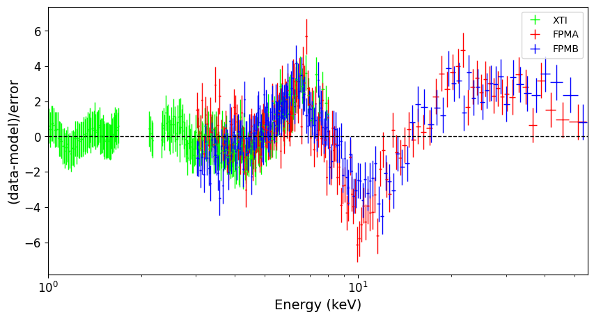
Figure 1: Normalized residuals for an absorbed power-law spectrum + disk blackbody spectrum [in XSPEC language, tbabs$\times$(diskbb+powerlaw)]. Green crosses are for XTI/NICER data, red crosses are for FPMA/NuSTAR data, and blue crosses are for FPMB/NuSTAR data. Data have been rebinned for visual clarity.

2.2 Data reduction

The raw data obtained from the NuSTAR detectors, denoted as FPMA and FPMB, are processed by the standard pipeline NUPIPELINE 0.4.9 in HEASOFT v6.32 using the latest calibration database CALDB v20230816. The Good time interval (GTI) files are produced using nuscreen, and we remove some obvious variabilities in the NuSTAR light curve by tool fv to preclude the impact of flare and dip events on the spectrum analysis. The source events are extracted from a circular region centered on MAXI J1803-298 with a radius of $120^{\prime\prime}$. The background region is a circle of the same size taken far from the source region to avoid any contribution from the source. We use the nuproducts to generate the spectra and other products. The FPMA and FPMB spectra are grouped to have a minimum count of 25 photons per bin for the chi-squared statistics to be applicable. The NuSTAR data are modeled over the 3–55 keV band for further analysis.

Based on the latest calibration file, the NICER data are processed following the standard steps. We use the tool nicer12 and nibackgen3C50 to extract the source and background spectra, respectively. The response matrix and ancillary file are generated by nicerrmf and nicerarf. In this work, the spectrum from NICER’s data is fitted over the energy band of 1.0-8.0 keV, ignoring the energy range of 1.7-2.1 keV (calibration residuals remain found in Si band) and 2.2-2.3 keV (calibration residuals remain in Au edges), respectively. We also group the XTI spectra to have a minimum count of 25 photons per bin.

3 Spectrum Analysis

Spectra are modeled using XSPEC v12.13.1 with $\chi^{2}$ statistics. To fit these spectra simultaneously from FPMA, FPMB, and XTI, a constant multiplicative factor was included in each model, set to 1.0 for XTI, and allowed to vary freely for FPMA and FPMB to eliminate the calibration differences in different instruments in the process of joint fit. To begin with, We fit the NuSTAR spectrum with a galactic absorbed power-law component from the corona and a thermal spectrum from the disk. The normalized residual is shown in Figure 1. This residual presents a strong reflection feature with a broad iron line around 6.4 keV and a Compton hump with a peak at 20-30 keV, with $\chi^{2}_{\nu}=3127.37/2290$.

Table 2: Best-fit Values for the Kerr Model I1-I4.

	Parameter	Model I1	Model I2	Model I2${}^{+}$	Model I3	Model I4
tbabs
$N_{H}(10^{21}cm^{-2}$)	Hydrogen column density	$3.68\pm 0.04$	$3.39\pm 0.07$	$3.54\pm 0.12$	$3.31\pm 0.04$	$3.16\pm 0.06$
diskbb
$T_{in}(keV)$	Temperature of disk	$0.813\pm 0.017$	$0.768\pm 0.007$	$0.822\pm 0.009$	$0.765\pm 0.005$	$0.793\pm 0.010$
$N_{diskbb}$	Normalization	$425\pm 43$	$612\pm 30$	$433\pm 31$	$598\pm 19$	$546\pm 33$
relxill flavor		relxill	relxillCP	relxillCP	relxilllp	relxilllpCP
h	Height of the corona	$-$	$-$	$-$	$<11.7$	$<10.8$
$q_{in}$	Emissivity index in the inner region	$10.0_{-4.9}$	$9.64_{-2.1}$	$10.0_{-5.09}$	$-$	$-$
$q_{out}$	Emissivity index in the outer region	$5.7\pm 5.7$	$6^{*}$	$6^{*}$	$-$	$-$
$R_{r}$(M)	Break radius	$2.13\pm 1.07$	$2.37\pm 0.79$	$2.15\pm 0.30$	$-$	$-$
$a^{*}$	Black hole spin	$0.989\pm 0.005$	$0.993\pm 0.007$	$0.984\pm 0.006$	$0.998^{*}$	$0.998^{*}$
$i$(deg)	Inclination angle	$72.5\pm 1.5$	$72.5\pm 1.8$	$68.2\pm 1.7$	$50.3\pm 2.2$	$44.1\pm 1.9$
$R_{in}$	Disk inner radius	$-1^{*}$	$-1^{*}$	$-1^{*}$	$-1^{*}$	$-1^{*}$
$\Gamma$	Photon Index	$2.34\pm 0.03$	$2.25\pm 0.02$	$2.22\pm 0.05$	$2.23\pm 0.02$	$2.17\pm 0.04$
$log\xi$	Ionization state of disk	$3.78\pm 0.28$	$4.44\pm 0.21$	$3.35\pm 0.09$	$4.70\pm 0.19$	$3.97\pm 0.14$
$logN$	The density of the accretion disk	$15^{*}$	$15^{*}$	$18.3\pm 0.5$	$15^{*}$	$18.0\pm 0.6$
$Fe$	Iron abundance	$1.17\pm 0.42$	$5.63\pm 2.90$	$1.30\pm 0.28$	$7.07\pm 2.19$	$4.35\pm 1.60$
$E_{cut}(kT_{e})(keV)$	Energy cut-off (or $T_{corona}$)	$300^{*}$	$100^{*}$	$100^{*}$	$300^{*}$	$100^{*}$
$R_{f}$	Reflection fraction	$1.92\pm 0.87$	$1.77\pm 0.52$	$1.74\pm 0.47$	$1.16\pm 0.42$	$0.66\pm 0.38$
$norm(10^{-2})$	Normalization	$1.9\pm 0.4$	$1.5\pm 0.2$	$1.2\pm 0.3$	$2.0\pm 0.7$	$2.2\pm 1.2$
gaussian
$E_{line}$	Absorption line energy in keV	$7.12\pm 0.06$	$7.11\pm 0.07$	$7.11\pm 0.06$	$7.33\pm 0.10$	$7.06\pm 0.10$
$\sigma_{E}$	Line width in keV	$0.08\pm 0.09$	$0.06\pm 0.10$	$0.08\pm 0.08$	$0.51\pm 0.11$	$0.78\pm 0.07$
$C_{FPMA}$	Cross-normalization	$1.023$	$1.023$	$1.023$	$1.023$	$1.024$
$C_{FPMB}$	Cross-normalization	$0.996$	$0.997$	$0.997$	$0.997$	$0.997$
$\chi^{2}/\nu$(reduced)	$-$	$2520/2279$	$2545/2280$	$2492/2279$	$2509/2282$	$2507/2281$
		$=1.106$	$=1.116$	$=1.093$	$=1.099$	$=1.099$

Note. — Best-fit values of initial Model I1-I4: $\texttt{tbabs}\times(\texttt{diskbb}+{\texttt{relxill(flavor)}}+\texttt{gaussian})$, in Xspec language (relxill, relxillCP, relxillp and relxillpCP, respectively), with errors calculated within a 90% confidence interval by $\chi^{2}$ statistic. $*$ indicates that the parameter is frozen in the fit. ${}^{+}$ indicates that the parameter $logN$ is free. $R_{in}=-1$ means that $R_{in}$ is set at the ISCO radius. The radial coordinate of the outer edge of the accretion disk is fixed at 400. $i$ is allowed to vary from $3^{\circ}$ to $80^{\circ}$. $a^{*}$ is allowed to vary from $-0.998$ to $0.998$. $logN$ in relxillCP flavors are allowed to range from 15 to 19. When the lower/upper uncertainty is not reported, the 90% confidence level reaches the boundary (or the best-fit is at the boundary).

To study the strong relativistic reflection composition in this source, our primary full XSPEC model involves substituting the power-law component with standard reflection models, denoted as relxill(flavor), which encompasses relxill, relxillCP, relxillp, and relxillpCP. The initial model is described by $\texttt{constant}\times\texttt{tbabs}\times(\texttt{diskbb}+{\texttt{relxill(flavor)}})$, where the specific flavors are respectively marked as I1-I4. tbabs describes the galactic absorption and has only one parameter; column density ($N_{H}$) along the line of sight. $N_{H}$ is set to be free while fitting the spectra. diskbb describes the thermal spectrum from the accretion disk. relxill(flavor) component describes the power-law and reflection composition. As it is widely believed that the accretion disk approaches the ISCO between the intermediate and soft states, we assume that the inner edge of the accretion disk is at the ISCO (equal to $6GM/c^{2}=6R_{g}$ for a Schwarzchild BH, or just 1 $R_{g}$ for a maximally spinning Kerr BH), and the outer radius is set to 400 $R_{g}$ where $R_{g}$ is the gravitational radius. The emissivity profile in model I1-I2 is modeled with a broken power-law emissivity profile with three parameters, and let them to free. Due to the limited fitting energy range, we additionally set the electron temperature of the corona (kTe) to 1/3 of the default value of the power law cutoff energy ($E_{cut}$ = 300 keV), i.e., kTe = 100 keV. Because inclination is measured by a high value from the same and another NuSTAR’s observation from feng2022spin and coughenour2023reflection, we also left it free to vary in the same way. In the lamppost model I3 and I4, we freeze the spin parameter to 0.998. Besides, a Fe XXVI absorption line at 7.0 keV has been detected during its intermediate state in zhang2024diskwinds, we also added a gaussian component in our model I1-I4.

After fitting the data with the model, we found the ”standard” weighting scheme in XSPEC often resulted in overfitting the data, yielding a reduced $\chi^{2}<1$. This is a known issue discussed in galloway2020multi regarding handling the low-count bins in XSPEC v.12. The Churazov weighting scheme is an alternative to the standard weighting used for fitting data (churazov1996mapping). It adjusts the weight by taking into account the counts in neighboring channels. This ensures that local extrema are not given disproportionate weight, leading to a smoother overall weighting. The result is a more accurate and reliable data fitting. Our best-fit results of Model I1-I4 are shown in Table 2, and all errors are reported at the 90% credible level.

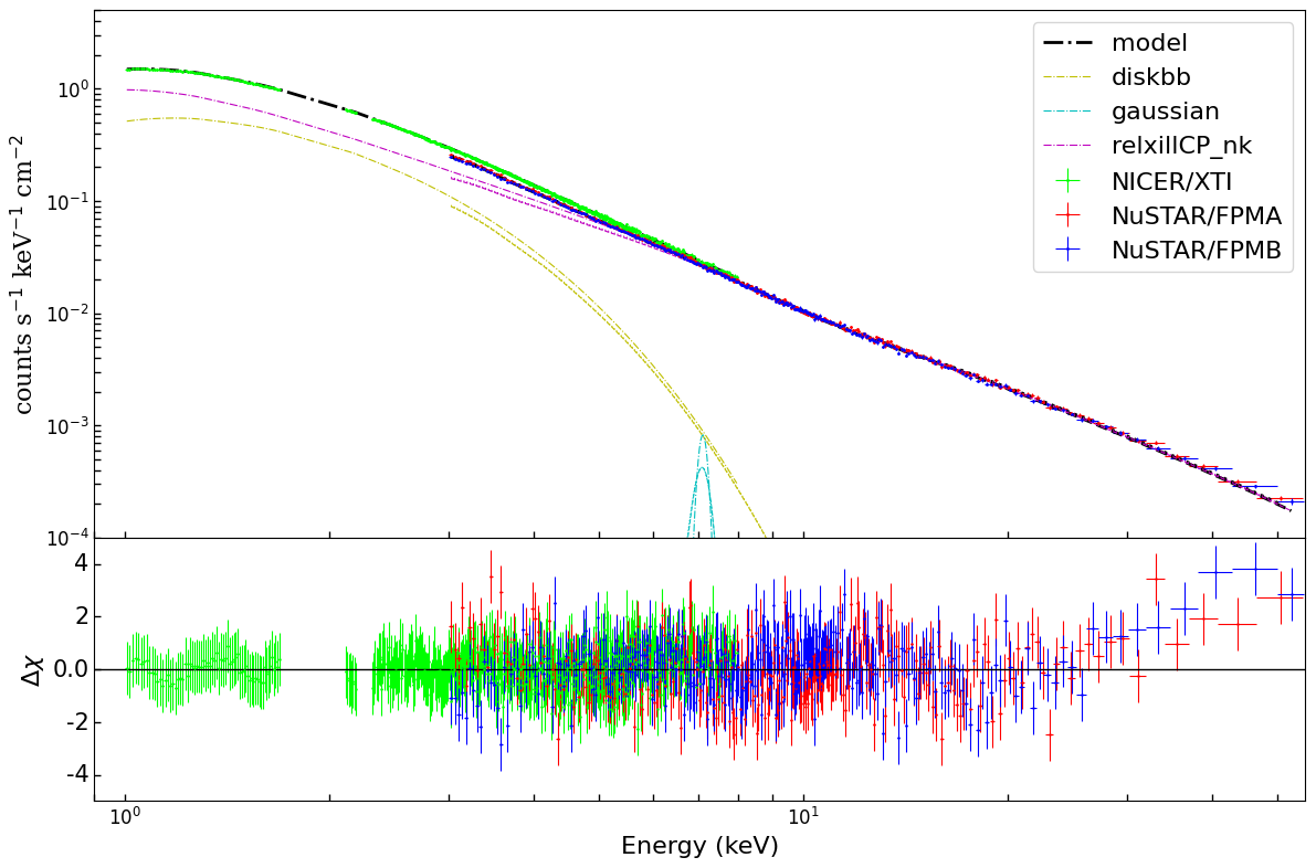
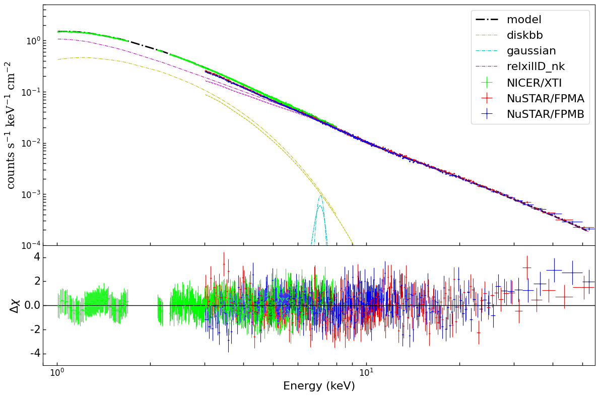
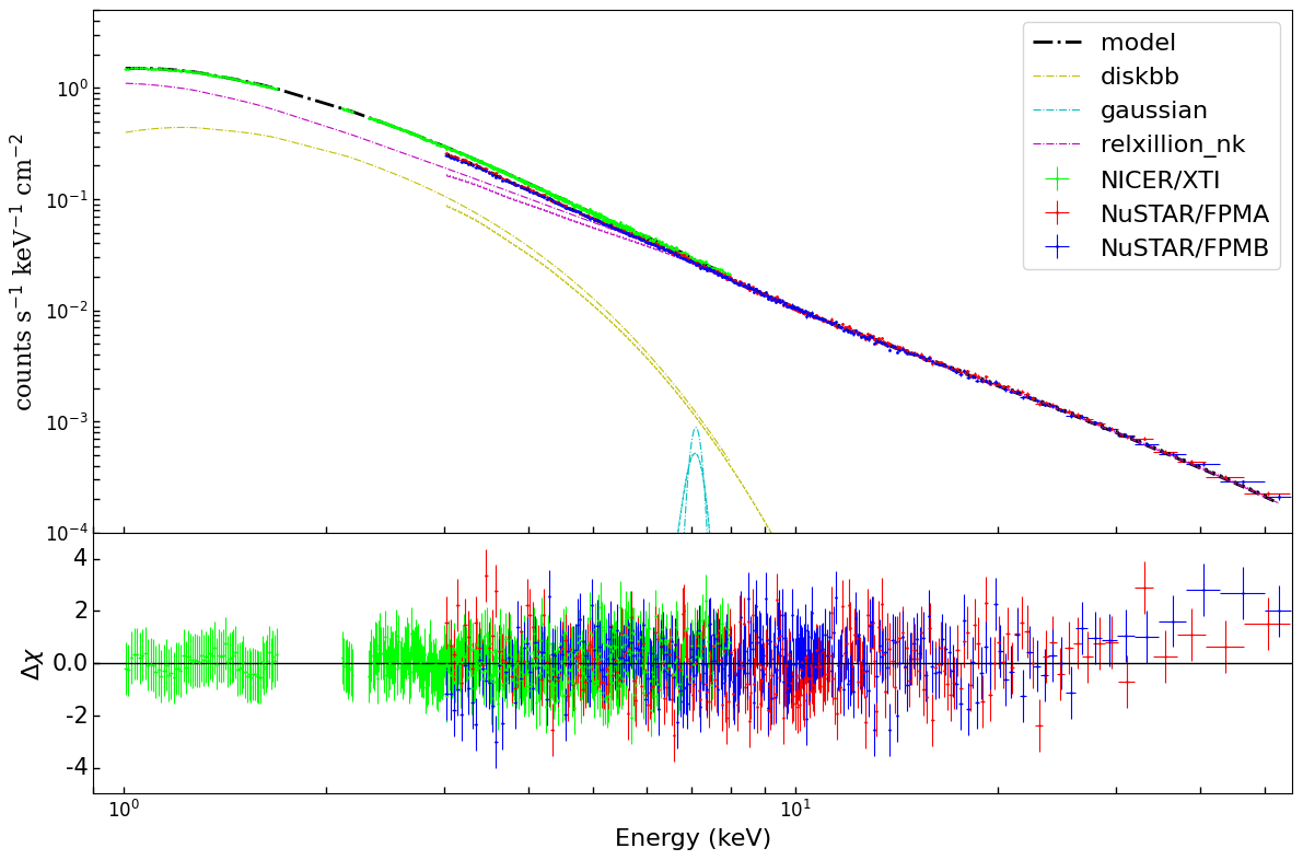
Figure 2: The best-fit results of unfolded spectra and normalized residuals of Model B1-B4. Upper quadrants show total models (black), relxill_nk (magenta), and diskbb (yellow). For each subgraph, dash-dot, dotted, and dashed lines present the same model for NICER/XTI, NuSTAR/FPMA, and NuSTAR/FPMB data, respectively. Lower quadrants show normalized residuals. NICER/XTI, NuSTAR/FPMA, and NuSTAR/FPMB data are plotted in green, red, and blue, respectively. Data have been rebinned for visual clarity.

We then substitute the relxill(flavors) model with various relxill_nk flavors: the relxill_nk (default model), relxillCP_nk (nthcomp Comptonization for the coronal spectrum), relxillD_nk (variable disk electron density), and relxillion_nk (the value of the ionization parameter varies as the radial coordinate r increases). We conduct joint fitting on the data. The models in XSPEC language are constant$\times$tbabs$\times$(diskbb+relxill_nk(flavor)+gaussian), which are respectively marked as A1-A4 (set $\alpha_{13}$ to 0) and B1-B4 (set $\alpha_{13}$ to free). More details of the extension of the relxill_nk model can be found in abdikamalov2019public. We apply the same bounds to the emissivity profile and the break radius as we did for Model I1-I2.

Within the framework of Johannsen spacetime, it is assumed that, with the exception of $\alpha_{13}$, the remaining three deformation parameters, namely $\alpha_{22}$, $\epsilon_{3}$ and $\alpha_{52}$, are held constant at zero for simplicity in this work. Here, a non-zero former signifies the departure from the Kerr metric. After we free $\alpha_{13}$, the best-fit results from our model B1-B4 are shown in Table 3, and its unfolded spectra and normalized residuals are shown in Figure 2.

The chi-square statistics is employed to determine the best-fit parameters, serving as the prior distribution for Markov Chain Monte Carlo (MCMC) analysis in the fitting process. The MCMC samples were generated using the Goodman & Weare algorithm embedded in the XSPEC software. The chains were run with 40 walkers, each comprising 25000 iterations, with an initial burn-in phase of 1000 steps. Thus, a total of $1\times 10^{6}$ samples were obtained. The 90% confidence intervals, indicative of purely statistical uncertainties across the entire parameter chain, for the free parameters within the best-fit results of models B1-B4 derived from the MCMC simulations, are detailed in Table 3. Furthermore, Figure LABEL:fig:relxill_nk, LABEL:fig:relxillCP_nk, LABEL:fig:relxillD_nk, and LABEL:fig:relxillion_nk showcase corner plots illustrating the one- and two-dimensional projections of the posterior probability distributions for the relevant free parameters corresponding to Model B1-B4, respectively, as a result of the MCMC analysis.

4 Discussion and Conclusions

After scrutinizing the spectra of MAXI J1803-298 from NuSTAR and NICER utilizing state-of-art relativistic reflection models in the preceding section, we derived precise and accurate constraints within these models employed in the present work. Our findings and conclusions are presented below.

In this work, we mainly used the relxill flavors and relxill_nk flavors to fit the data. Our best-fit values of our employed models I1-I4 and A1-B6 are shown in Table 2 and Table 3, respectively. It is essential to recognize that direct comparisons of the $\chi^{2}$ values between Models I1-I4 utilizing relxill flavors and Models A1-B6 employing relxill_nk flavors cannot definitively ascertain the superior model due to variations in the calculation of the transfer function. As such, the minor discrepancies observed in the $\chi^{2}$ values between these two sets of models will not impact the subsequent discussion.

4.1 Fitting with Relxill Flavors

We first compare our best-fit results of model A with results shown on feng2022spin. Our findings showcase a relatively lower galactic absorption coefficient$\sim 3.0\times 10^{21}cm^{-1}$, which aligns with results in Homan2021ATel. However, the best-fit values in Table 2 show a slightly higher galactic absorption coefficient than the results in chandApJHIS, which may be caused by the outflowing disk winds and the moving clouds during the outburst.

In the initial model I1-I2, the results obtained with relxill and relxillCP, which are standard models for relativistic reflection within the Kerr paradigm, incorporate emissivity that can be parameterized either through an empirically defined broken power law. Our results shown in Table 2, indicative of a black hole with extremely high spin and a highly inclined accretion disk (approximately $70^{\circ}$). Particularly, there shows $\Delta\chi^{2}>45$ when the density of the accretion disk is set free, denoted to Model I2${}^{+}$. This suggests a high ionization density disk near $\sim 10^{18}$ cm${}^{-3}$, within MAXI J1803-298, which aligns with coughenour2023reflection. Thus, their fit results with a higher galactic absorption coefficient $\sim 5.0\times 10^{21}$ cm${}^{-1}$ with only a low ionization density disk model relxillCP in feng2022spin appear to be inconclusive.

We subsequently incorporate lamppost models I3 and I4, which posit a lamppost source located along the rotational axis, to evaluate the proximity of the corona to the disk, setting the spin parameter to 0.998. The results indicate that the height of the compact corona above the disk is constrained to $h<10.8R_{g}$, suggesting a still pronounced reflection component in the data observed during its SIMS.

4.2 Fitting with Relxill_nk Flavors

Afterward, we transition to the relxill_nk flavors to investigate the correlation between deformation parameters $\alpha_{13}$ and the spin parameter $a^{*}$ based on its reflection feature. As is shown in model B1-B4 in Table 3, it is evident that when modeling the emissivity profile with a broken power law using the relxill_nk flavors, consistently high spin values ($a^{*}>0.98$) are observed. Additionally, there is a notable pattern of high values for the emissivity index $q_{in}$ and low values for $q_{out}$. This further supports our fit results of a compact corona near the black hole modeled by Model I3-I4 in Section 4.1.

In model B2 with relxillCP_nk, in which the parameter $kT_{e}$ represents the temperature of the corona, we found a stringent constraint on the deformation parameter assuming the Johannsen spacetime (johannsen2013regular). However, this constraint on $\alpha_{13}$ should be excluded due to its bad parameter estimation, details are presented in Section 4.3. In addition, since the electron density is fixed to a low value of $10^{15}$ cm${}^{-3}$ rather than a high disk density in the disk in Model B1 and Model B2. We employed relxillD_nk for data fitting, where the parameter linked to the disk electron density, $logN$, which was frozen to 18 due to the high disk density we got from Model I2${}^{+}$ in section 4.1. Notably, when the high disk density is set to 18 in Model B3, it shows $\Delta\chi^{2}>14$, but it will not significantly change the constraint on $\alpha_{13}$. The contours of spin versus deformation parameter $\alpha_{13}$ are shown in Figure LABEL:fig:a13_a.

In previous relxill_nk flavors, the ionization parameter $\xi$ was not considered as a variable. To address this, we also applied the relxillion_nk model (abdikamalov2021implementation), utilizing xillver table for the reflection spectrum in the rest-frame of the gas. In this model, the electron density is assumed to be a constant ($10^{15}$ cm${}^{-3}$) across the entire disk. The ionization has instead a radial profile described by a power law

$$\xi(r)=\xi_{\mathrm{in}}\left(\frac{R_{\mathrm{in}}}{r}\right)^{\alpha_{\xi}}.$$ (1)

For the index of $\alpha_{\xi}=0$, model relxillion_nk is reduced to relxill_nk. Our best-fit result from model B4 indicates a positive value of $\alpha_{\xi}$, which shows the $\Delta\chi^{2}>80$ compared with Model B1, implying that the ionization parameter decreases as the radial coordinate $r$ increases within the actual disk.

4.3 The Best-fit Model

Among the initial models I1-I4 with deferent relxill flavors, Model I2${}^{+}$ shows the best-fit results modeled by a high density disk, approximately 10${}^{18}$ cm${}^{-3}$. From the residuals of Model B1-B4 shown in Figure 2, there are no significant differences among their fits. However, there is a slight elevation in the residuals above 30 keV among Models B1-B4. We attribute this behavior to a low count rate above 30 keV during the soft intermediate state. If we compare their $\chi^{2}$, we see that model B4 best fits MAXI J1803-298, and its value of the ionization index is near 0.5. However, comparing the minimum of $\chi^{2}$ of different models is not a particularly robust method to determine which model is favored by the data. AIC (Akaike Information Criterion) (akaike1974new), which is already applied and discussed in mall2022impact, is a more reliable method to determine the best model in this case of a relatively small size of samples for the number of free parameters. As we already have the minimum $\chi^{2}$ for every model by XSPEC, it can be calculated the AICc straightly by

$$\mathrm{AICc}=\chi_{\min}^{2}+2N_{p}+\frac{2N_{p}\left(N_{p}+1\right)}{\left(N_{b}-N_{p}-1\right)},$$ (2)

where $N_{p}$ is the number of free parameters, and $N_{b}$ is the number of bins. The values of AICc obtained from Model A1-A3 and Model B1-B4 are shown in Table LABEL:tab:AICc. As a general criterion for AIC, models with $\Delta AICc>5$ are considered less favored by the data, while those with $\Delta AICc>10$ are deemed ruled out and can be excluded from further analysis (burnham2004model).

By applying this selection criterion, we determine that among Models A1-A3, Model I2${}^{+}$, which incorporates a high-density disk, achieves the best fit. Among Models B1-B4, the relxillion_nk model distinctly outperforms the other three in terms of fit quality. Despite we found a precise constraint on $\alpha_{13}=0.002^{+0.020}_{-0.015}$ with relxillCP_nk, at a 3-$\sigma$ confidence level, Model B2 is deemed unsuitable for consideration. This is due to its fixed corona electron temperature at 100 keV and unrealistic estimates of certain parameters, such as $A_{Fe}$ and $log\xi$. Notably, the fits where $kT_{e}$ is allowed to vary, it invariably maxes out at 400 keV. Consequently, the outcomes from Models A2 and B2 are excluded from our analysis, not merely because of their elevated reduced $\chi^{2}$ values but also due to the low disk density values inserted. Considering the AICc values presented in Table LABEL:tab:AICc and their plausible parameter estimates, Models B3 and B4 are affirmed as providing more reliable constraints on $\alpha_{13}$.

Table 3: Summary of the Best-fit Values for Johannsen Models A1-B6 with only set free $\alpha_{13}$ after the MCMC Runs

	Model A1	Model B1	Model A2	Model B2	Model A3	Model B3	Model A4	Model B4	Model B5	Model B6
tbabs
$N_{H}(10^{21}cm^{-2}$)	$3.35^{+0.04}_{-0.08}$	$3.34^{+0.04}_{-0.03}$	$3.22^{+0.04}_{-0.03}$	$3.20^{+0.02}_{-0.03}$	$3.33^{+0.06}_{-0.05}$	$3.33^{+0.05}_{-0.04}$	$3.60^{+0.05}_{-0.06}$	$3.58^{+0.08}_{-0.06}$	$3.50^{+0.03}_{-0.06}$	$3.28^{+0.03}_{-0.03}$
diskbb
$T_{in}(keV)$	$0.765^{+0.006}_{-0.015}$	$0.783^{+0.003}_{-0.003}$	$0.746^{+0.004}_{-0.003}$	$0.745^{+0.004}_{-0.004}$	$0.774^{+0.005}_{-0.005}$	$0.777^{+0.006}_{-0.007}$	$0.808^{+0.007}_{-0.008}$	$0.804^{+0.012}_{-0.008}$	$0.787^{+0.004}_{-0.003}$	$0.755^{+0.002}_{-0.004}$
$N_{diskbb}$	$606^{+53}_{-20}$	$599^{+14}_{-25}$	$702^{+14}_{-20}$	$714^{+15}_{-18}$	$564^{+27}_{-22}$	$567^{+16}_{-41}$	$430^{+31}_{-24}$	$438^{+36}_{-37}$	$496^{+15}_{-18}$	$645^{+14}_{-9}$
relxill_nk flavor	relxill_nk		relxillCP_nk		relxillD_nk		relxillion_nk		relxill_nk
	$\alpha_{13}=0$	free $\alpha_{13}$	$\alpha_{13}=0$	free $\alpha_{13}$	$\alpha_{13}=0$	free $\alpha_{13}$	$\alpha_{13}=0$	free $\alpha_{13}$	set Fe=1	set Fe=5
$q_{in}$	$10^{*}$	$10^{*}$	$9.76_{-0.92}$	$9.73_{-0.91}$	$9.94_{-0.49}$	$9.94_{-2.3}$	$9.73_{-0.89}$	$9.96_{-1.10}$	$9.94_{-2.42}$	$9.94_{-2.26}$
$q_{out}$	$1.62^{+0.75}_{-0.38}$	$1.83^{+0.44}_{-0.93}$	$2.02^{+0.26}_{-0.18}$	$2.09^{+0.27}_{-0.25}$	$1.60^{+0.30}_{-0.28}$	$1.66^{+0.35}_{-0.56}$	$1.24^{+0.35}_{-0.35}$	$1.06^{+0.32}_{-0.55}$	$1.64^{+0.37}_{-0.77}$	$2.11^{+0.91}_{-1.21}$
$R_{r}$(M)	$2.97^{+0.47}_{-0.25}$	$2.85^{+1.36}_{-0.07}$	$2.83^{+0.15}_{-0.11}$	$2.80^{+0.33}_{-0.15}$	$3.06^{+0.42}_{-0.20}$	$3.36^{+0.93}_{-0.36}$	$3.97^{+0.43}_{-0.49}$	$4.04^{+1.09}_{-0.42}$	$2.97^{+1.27}_{-0.33}$	$2.99^{+2.02}_{-0.13}$
$a^{*}$	$0.993_{-0.011}$	$0.994_{-0.012}$	$0.995^{+0.002}_{-0.005}$	$0.997^{+0.001}_{-0.002}$	$0.992_{-0.005}$	$0.992_{-0.010}$	$0.988^{+0.004}_{-0.004}$	$0.993_{-0.007}$	$0.997_{-0.001}$	$0.995_{-0.009}$
$i$(deg)	$71.1^{+3.0}_{-3.4}$	$73.7^{+1.2}_{-9.4}$	$69.2^{+2.8}_{-6.5}$	$69.7^{+3.1}_{-3.1}$	$69.5^{+2.6}_{-5.4}$	$67.3^{+4.1}_{-9.8}$	$74.4^{+2.5}_{-2.4}$	$75.9^{+2.1}_{-3.3}$	$72.1^{+4.4}_{-3.9}$	$71.1^{+3.9}_{-6.1}$
$R_{in}$	$-1^{*}$	$-1^{*}$	$-1^{*}$	$-1^{*}$	$-1^{*}$	$-1^{*}$	$-1^{*}$	$-1^{*}$	$-1^{*}$	$-1^{*}$
$\Gamma$	$2.203^{+0.013}_{-0.042}$	$2.204^{+0.023}_{-0.006}$	$2.187^{+0.013}_{-0.006}$	$2.178^{+0.008}_{-0.008}$	$2.194^{+0.012}_{-0.011}$	$2.200^{+0.020}_{-0.009}$	$2.319^{+0.016}_{-0.021}$	$2.317^{+0.016}_{-0.020}$	$2.271^{+0.010}_{-0.011}$	$2.190^{+0.006}_{-0.008}$
$log\xi$	$4.29^{+0.25}_{-0.07}$	$4.30^{+0.02}_{-0.09}$	$4.84^{+0.10}_{-0.09}$	$4.80^{+0.12}_{-0.12}$	$4.07^{+0.07}_{-0.06}$	$4.07^{+0.07}_{-0.05}$	$4.41^{+0.08}_{-0.07}$	$4.38^{+0.08}_{-0.08}$	$4.08^{+0.05}_{-0.03}$	$4.49^{+0.04}_{-0.04}$
$A_{Fe}$	$2.83^{+1.55}_{-0.50}$	$2.71^{+0.32}_{-0.47}$	$8.55^{+0.62}_{-0.94}$	$8.64^{+1.05}_{-0.98}$	$2.02^{+0.50}_{-0.31}$	$1.89^{+0.61}_{-0.39}$	$1.41^{+0.46}_{-0.32}$	$1.31^{+0.71}_{-0.30}$	$1^{*}$	$5^{*}$
$E_{cut}(kT_{e})(keV)$	$300^{*}$	$300^{*}$	$100^{*}$	$100^{*}$	$300^{*}$	$300^{*}$	$300^{*}$	$300^{*}$	$300^{*}$	$300^{*}$
$logN(cm^{-3})$	$15^{*}$	$15^{*}$	$15^{*}$	$15^{*}$	$18^{*}$	$18^{*}$	$15^{*}$		$15^{*}$	$15^{*}$
$\alpha_{\xi}$	$0^{*}$	$0^{*}$	$0^{*}$	$0^{*}$	$0^{*}$	$0^{*}$	$0.54^{+0.04}_{-0.04}$	$0.52^{+0.03}_{-0.04}$	$0^{*}$	$0^{*}$
$\alpha_{13}$	$0^{*}$	$0.029^{+0.043}_{-0.040}$	$0^{*}$	$0.002^{+0.021}_{-0.011}$	$0^{*}$	$0.023^{+0.050}_{-0.031}$	$0^{*}$	$0.006^{+0.038}_{-0.016}$	$0.026^{+0.051}_{-0.050}$	$0.032^{+0.034}_{-0.037}$
$R_{f}$	$1.87^{+0.76}_{-0.64}$	$1.42^{+0.56}_{-0.20}$	$0.92^{+0.20}_{-0.17}$	$1.07^{+0.09}_{-0.16}$	$1.64^{+0.14}_{-0.16}$	$1.03^{+0.40}_{-0.16}$	$0.96^{+0.12}_{-0.10}$	$0.98^{+0.30}_{-0.19}$	$1.47^{+0.69}_{-0.14}$	$1.25^{+0.46}_{-0.11}$
$norm(10^{-3})$	$3.9^{+2.1}_{-1.9}$	$4.1^{+2.3}_{-1.4}$	$7.0^{+1.8}_{-1.7}$	$6.2^{+1.8}_{-1.5}$	$4.7^{+2.8}_{-1.7}$	$5.6^{+1.4}_{-0.8}$	$8.3^{+4.3}_{-4.6}$	$7.5^{+4.2}_{-3.7}$	$4.2^{+2.1}_{-3.2}$	$3.9^{+2.5}_{-3.1}$
gaussian
$\sigma_{line}$	$<0.31$	$<0.47$	$<0.13$	$<0.12$	$<0.33$	$<0.35$	$<0.53$	$<0.56$	$<0.41$	$<0.35$
$Norm(10^{-4})$	$-3.1$	$-2.6$	$-3.0$	$-2.3$	$-4.1$	$-3.2$	$-3.1$	$-3.0$	$-2.6$	$-2.2$
$C_{FPMA}$	$1.023$	$1.023$	$1.023$	$1.023$	$1.023$	$1.023$	$1.023$	$1.023$	$1.022$	$1.023$
$C_{FPMB}$	$0.996$	$0.997$	$0.997$	$0.995$	$0.997$	$0.997$	$0.997$	$0.997$	$0.997$	$0.997$
$\chi^{2}/\nu$(reduced)	$2533/2281$	$2527/2280$	$2563/2280$	$2565/2279$	$2521/2280$	$2513/2279$	$2446/2279$	$2444/2278$	$2567/2280$	$2533/2280$
	$=1.110$	$=1.108$	$=1.124$	$=1.125$	$=1.105$	$=1.103$	$=1.073$	$=1.072$	$=1.125$	$=1.111$

Note. — Best-fit Values of Model A1-B6(includes relxill_nk, relxillCP_nk, relxillD_nk, and relxillion_nk). All errors determined through a 90% confidence interval after MCMC runs for the global minimum. $*$ indicates that the parameter is frozen in the fit. $R_{in}=-1$ means that $R_{in}$ is set at the ISCO radius. The radial coordinate of the outer edge of the accretion disk is fixed to 400. $i$ is allowed to vary from $3^{\circ}$ to $80^{\circ}$. $a^{*}$ is allowed to vary from $-0.998$ to $0.998$. The deformation parameters of $\alpha_{13}$ is allowed to vary from $-1$ to 1. $E_{line}$ in gaussian is frozen to 7.1 keV. When the lower/upper uncertainty is not reported, the 90% confidence level reaches the boundary (or the best-fit is at the boundary).