Robust Advertisement Pricing
Click here for the latest version

Abstract

We consider the robust pricing problem of an advertising platform that charges a producer for disclosing hard evidence of product quality to a consumer before trading. Multiple equilibria arise since consumer beliefs and producer’s contingent advertisement purchases are interdependent. To tackle strategic uncertainty, the platform offers each producer’s quality type a menu of disclosure-probability-and-price plans to maximize its revenue guaranteed across all equilibria. The optimal menus offer a continuum of plans with strictly increasing marginal prices for higher disclosure probabilities. Full disclosure is implemented in the unique equilibrium. All partial-disclosure plans, though off-path, preclude bad equilibrium play. This solution admits a tractable price function that suggests volume-based pricing can outperform click-based pricing when strategic uncertainty is accounted for. Moreover, the platform prioritizes attracting higher types into service and offers them higher rents despite symmetric information between the platform and the producer.

JEL codes: D47, D82, D86, L86, M37

Keywords: verifiable disclosure, advertisement pricing, contracting with externalities, adversarial equilibrium selection, divide and conquer

1 Introduction

Search engines, social media, and e-commerce platforms offer ad plans that enable producers to disclose product information to consumers to affect product prices. A crucial issue is that consumers often cannot observe the producers’ ad plan choices; they only see the ads if the platforms distribute them. This leads to consumer skepticism: When consumers find themselves unexposed to any ad, they cannot distinguish between a producer investing little on ads and one investing heavily yet unable to reach out to them.

A key problem of strategic uncertainty thus arises: Consumer skepticism depends on how much consumers expect the producers to spend on ads contingent on product quality; In turn, such skepticism also endogenously determines the producers’ outside value of not purchasing ads, consequently influencing their contingent purchase decisions. Different consumer skepticism can be self-fulfilling and there may be multiple equilibria, some of which lead to extremely low revenue for the platform.

In the presence of such strategic uncertainty, this paper studies a platform’s optimal design of advertisement pricing that maximizes the revenue guarantee across all equilibria. We ask: What is the robustly optimal pricing scheme? How much surplus is left for producers? Should the platform hide information intentionally? Does our solution speak to the prolonged discussion on the modeling of ad prices/costs?

In our model, a producer acquires hard evidence that reveals the quality of her product. For example, the producer can obtain hard evidence through awards, test certificates, product reviews/ratings However, the producer cannot disclose the hard evidence to a (representative) consumer by herself. This may be because the producer cannot attract consumer attention, or because it is too costly for each individual consumer to verify the hard evidence. The only way the producer can disclose product information to the consumer is to purchase the ad services offered by a platform. To profit from advertising, the platform designs a profile of menus that contain ad plans. Each plan consists of a (potentially interior) disclosure probability and a price. Since the evidence is usually needed for producing ads, we assume the platform can directly observe the producer’s type and offer type-dependent menus of ad plans. In this way, we eliminate adverse selection as a confounding driving force in the model.

Given any profile of type-dependent menus, a game between the producer and the consumer unfolds as follows. First, the hard evidence is realized and observed by both the producer and the platform. The producer can either choose no disclosure or pick one plan from the menu exclusive to her type. Crucially, the producer’s choice is not observed by the consumer. If a plan is chosen, the platform charges the price and stochastically discloses the evidence with the probability specified in the chosen plan. Upon seeing the evidence, the consumer learns the type. If disclosure does not happen, the consumer updates belief according to his conjecture of the producer’s contingent purchase decisions. Finally, the producer sells the product to the consumer via a take-it-or-leave-it offer at a price equal to his posterior mean.

There may be multiple equilibria between the producer and the consumer. To illustrate how severe the issue of strategic uncertainty can be in our environment and motivate our robust objective, let us start with the benchmark where the platform can select its favorite equilibrium as in standard principal-agent frameworks. In this case, the optimal pricing policy for the platform is to sell full disclosure to producers of any type $\theta$ except the lowest type $\underline{\theta}$ at the price $\theta-\underline{\theta}$. In the induced platform’s favorite equilibrium, producers of all types except the lowest type $\underline{\theta}$ pay for full disclosure. The consumer skepticism in this equilibrium is rather extreme: When the consumer sees no ads, he believes the product has the lowest quality. This extreme skepticism serves as the most powerful punishment against producers who turn down the platform’s offer by giving them an outside value of $\underline{\theta}$. The platform can thus achieve maximum possible surplus extraction. However, under the same pricing design, there is an extremely undesirable equilibrium for the platform where it earns zero revenue. In this equilibrium, no producers of any type purchase the ad, and the consumer skepticism belief remains the prior. This mild skepticism means the producer can sell the product at a price equal to the prior mean $\mathbb{E}[\theta]$ without advertising, so she has no incentives to purchase the expensive full disclosure.

The stark difference in the revenue among multiple equilibria suggests that the platform faces large strategic uncertainty. In fact, we can show a stronger result: For any pricing policy that achieves close to full-surplus extraction in the platform’s favorite equilibrium, the pricing policy also induces a bad equilibrium where the platform’s revenue is close to 0. To the extent that the platform in our model does not create social surplus, it may especially worry that the producer and the consumer coordinate on its least favorite equilibrium to resist surplus extraction. Moreover, the platform may also worry that market participants cannot play Nash equilibrium and instead resort to weaker notions such as rationalizability.

With these motivations, we solve for the robustly optimal menu profile that guarantees the maximum expected revenue to the platform in the worst-case equilibrium of the induced producer-consumer game. The optimal solution also induces a unique rationalizable outcome, so it remains optimal if the objective is to maximize revenue guarantee among all rationalizable outcomes.

Our main result, Theorem 1, delivers two central characteristics of the robustly optimal menu profile: (i) The menu for each type contains a continuum of plans equivalent to a strictly convex price function, but most of plans are never chosen on the equilibrium path; (ii) The platform adopts a complete divide-and-conquer strategy by offering plans as if it always prioritizes guaranteeing disclosure probabilities from high types over low types.

One can visualize the robustly optimal menu profile through the following procedure: First, the platform uses a plan with a small disclosure probability with a sufficiently low price to bait the highest type producer to deviate from the hypothetical equilibrium where no type discloses. Then, it introduces a continuous sequence of similar bait plans. Each such bait plan lures the highest type out of the hypothetical equilibrium where she chooses the plan right before the bait plan in the sequence. Full disclosure hereby becomes the unique credible choice of the highest type. Next, this continuous baiting process repeats for the second highest type, but the hypothetical equilibria to be broken now take the highest type’s full disclosure as granted. After this, the process continues sequentially for the other lower types, assuming all higher types’ full disclosure as guaranteed.

Our first solution characteristic points out the optimality of using continuous off-path plans. Off-path plans are never chosen by the producer in the induced equilibrium, but they serve as baits to break undesirable equilibria. To provide intuitions for the result, we examine the following binary-type example. Consider a producer whose product is of value either 0 (low) or $\overline{\theta}=1$ (high), and each value occurs with equal probabilities. Since it is never profitable to induce the low type to disclose, we assume for now the platform offers a single menu exclusive to the high type.

To see why it is beneficial to offer more than one plan in the menu, let us start by solving the optimal single-plan menu. In this case, it is optimal to offer a full disclosure plan, and the high type must choose between purchasing the plan and ignoring the ads. To robustly induce full disclosure from the high type, the price of the full disclosure plan must be so low that the high type ignoring the ads cannot form an equilibrium. Suppose such under-advertising indeed forms an equilibrium, the consumer skepticism equals the prior, and the producer can sell the product with price $\frac{1}{2}$ without purchasing ads. Thus, to break the hypothetical equilibrium, the full disclosure price cannot exceed $1\times(\overline{\theta}-\frac{1}{2})=\frac{1}{2}$, where 1 is the disclosure probability, $\overline{\theta}$ and $\frac{1}{2}$ are the respective gains from reaching and not reaching the consumer via ads. In conclusion, the robust guarantee cannot exceed $\frac{1}{2}$ with single-plan menus.

However, the platform can do better by offering a second plan in the menu as follows. The menu offers a full disclosure plan with price $\frac{7}{12}-2\epsilon$ and a half disclosure plan (probability $\frac{1}{2}$) with price $\frac{1}{4}-\epsilon$. This menu induces full disclosure in the unique equilibrium and guarantees a revenue of $\frac{7}{12}-2\epsilon$, higher than the revenue of $\frac{1}{2}$ in the previous case. To see this, let us first consider the hypothetical equilibrium where the high type ignores the ads completely. Because observing no ads does not alter the consumer’s belief, the producer’s outside value is $\frac{1}{2}$. The price for half disclosure is strictly smaller than $\frac{1}{2}\times(\overline{\theta}-\frac{1}{2})=\frac{1}{4}$ so the high type finds it optimal to deviate to purchase the half disclosure plan. Next, consider the second hypothetical equilibrium where the high type chooses half disclosure. Importantly, since the high type producer does disclose in this hypothetical equilibrium, observing no ads becomes a bad signal: The consumer in skepticism believes that the high type only has probability $\frac{1}{3}$. This implies the producer’s outside value drops to $\frac{1}{3}$. Thus, the high type finds it profitable to deviate to full disclosure because the price increment from half to full disclosure is strictly smaller than $\frac{1}{2}\times(\overline{\theta}-\frac{1}{3})=\frac{1}{3}$.

As illustrated in the binary example, an interesting feature of the optimal solution is that the high-type producer is lured to “defeat herself”. In a hypothetical equilibrium where the high type has more disclosure, the consumer thinks worse of the producer in skepticism, creating a lower outside value for her. From above, one can see the outside value of $\frac{1}{3}$ in the half disclosure equilibrium is lower than that of $\frac{1}{2}$ in the ignore-the-ads equilibrium. However, the high type is always lured to deviate to a higher disclosure probability, failing to internalize the indirect externalities this has on herself. The example only shows how to move from a 1-plan menu to a 2-plan menu. One can imagine how to further improve the revenue guarantee by filling in more intermediate plans. As the number of plans grows to infinity, the menu converges to our optimal solution with a continuum of plans.

The intuition for the other solution characteristic, complete divide-and-conquer, is harder to deliver in short sentences. Roughly speaking, one can sense from the previous example that to robustly induce an additional unit of disclosure probability, the platform needs to compensate the producer for giving up her outside value, which equals the consumer’s value expectation in skepticism. Therefore, to reduce the total rent left to the producer while robustly inducing full disclosure, the platform wants to strike down consumer skepticism as “fast” as possible. The disclosure of higher types should be prioritized because the Bayes rule indicates that one unit of ex-ante disclosure probability from a higher type strikes down skepticism more effectively than that from a lower type. Thus, the complete divide-and-conquer strategy is optimal.

It is challenging to prove the optimality of our solution because worst-case implementation requires breaking all the undesirable equilibria and it is unclear what is the optimal way to break them. In other words, the platform has to answer two questions: In each undesirable equilibrium, which type of the producer deviates, and which plan does the type deviate to? We provide clear answers to these questions. Lemma 2 answers the second question by showing that it suffices to look at cases where each equilibrium is broken by some local upward deviation. Lemma 3 answers the first question and says that the deviating type should always be the highest type that has not yet fully disclosed herself.

Our main result gives rise to a couple of interesting implications. First, optimally countering strategic uncertainty does not lead to distortion in “allocations” as full disclosure is induced in the unique equilibrium. For comparison, other frictions such as adverse selection would rather induce inefficient communication. Second, under the optimal solution, producers of higher types enjoy higher rents. Such a monotonic rent structure comes from the optimality condition: Many suboptimal menu profiles induce non-monotonic rents. This contrasts with a setting where adverse selection is the main driving force and monotonic rents result from incentive compatibility. Third, the strictly convex price functions contrast with the well-known click-based pricing yet take a logarithm form that supports the classic volume-based pricing first developed by, for example, Butters (1977) and Grossman and Shapiro (1984).

To explore the allocative role of platform advertising, we first consider two benchmarks where the platform is absent and the producer either can or cannot control disclosure. If the producer cannot self-advertise, then no communication happens and every type earns the prior mean. If the producer does have the option to disclose freely, we have the setting of Grossman (1981) and Milgrom (1981) who show that, in equilibrium, the producer’s unraveling impetus results in every type fully disclosing and earning exactly the type. In both cases, the producer extracts full surplus, albeit distributed differently among types. In comparison, the platform in our model is able to extract high surplus despite adversarial equilibrium selection, and every producer type is strictly worse off than in both benchmarks.

Finally, we consider several robustness checks and extensions. First, we show that under the optimal menu profile, all types expect the lowest type choosing full disclosure is the unique rationalizable outcome so our solution remains robustly optimal even if the platform worries that market participants may fail to play Nash equilibrium.

Second, in the main model, the type-dependent menus are deterministic. We show this is without loss of generality and point out another way of implementing our optimal solution: Instead of offering a deterministic menu with continuous options, the platform can achieve the same by offering only the option of full disclosure at a random price. This implementation may work better in applications where the platform cannot completely control or fine-tune the disclosure probability.

Third, we allow the platform to jointly design the menu profile and the information structure. This extension speaks to applications where evidence about product value is generated and controlled by the platform. For example, Amazon extracts keywords from reviews and YouTube gives out creator awards. We show that the platform’s desire to strike down consumer skepticism as “fast” as possible makes it want to segregate the information. Consequently, perfect revealing is the optimal information structure. Fourth, we show that the producer types still face strictly convex price functions even if the platform needs to pay potentially non-convex advertising costs.

Outline. Section 2 lays out the model, entailing a benchmark case without strategic uncertainty and a discussion of assumptions. With a binary-type example, Section 3 illustrates the optimality of using continuous menus. Section 4.1 discusses our main result. Section 4.2 and Section 4.3 show three lemmas toward the proof and insights. Section 5 analyzes the extensions. All proofs are in the Appendix.

Literature Review

This paper relates to the literature on contracting with externalities in multi-agent settings, pioneered by Segal (1999, 2003). Our solution concept of robust optimum achieves unique implementation, as in most papers in this literature.

The most related paper is Segal (2003) who also studies settings where a principal offers bilateral agent-by-agent (in our case, type-by-type) menus of plans to implement the desired outcome in the unique equilibrium. Our major departure from him and all the others in this literature mentioned below is that the multiple producer types in our model have indirect externalities. In other words, one type’s disclosure will not directly affect other types’ payoffs but it can indirectly influence payoffs through shifting consumer beliefs. Put differently, the consumer’s skepticism belief is an equilibrium element that the platform can neither contract on nor provide incentives to. This key difference separates our solution that offers continuous menus from Segal’s solution where it suffices to use finite ones, even though both settings allow for continuous action spaces. Moreover, one result of Segal (2003), his Lemma 3, is related to our Lemma 2 in showing that every menu profile can be mapped into an alternating divide-and-conquer strategy. However, since we deal with plan continuums and do not have increasing externalities for all types, his Round-Robin optimization argument is not directly applicable.

Another branch of this literature led by Winter (2004) also seeks to weaken contractibility by limiting the principal’s ability to monitor agent actions and offer incentives to them. Many, such as Winter (2004), Bernstein and Winter (2012), and Halac et al. (2020), consider binary actions and simple monitoring systems, which results in the principal offering a single plan to each agent. Halac et al. (2021), Halac et al. (2022), and Halac et al. (2023) allow the principal to jointly design communication or monitoring schemes, which enriches the solution structure. In particular, Halac et al. (2021) study a principal who can offer stochastic contracts and privately inform each agent of his contract realization before choice-making. Their optimal contracts alternatingly divide-and-conquer the probabilities of agents taking actions. However, their solution shares a finite structure with Segal (2003). Our random menus extension (Section 5.3) interprets our optimal solution as random menus with continuous supports.

On the pricing of communication under adversarial equilibrium selection, Ali et al. (2022) study a rating agency that designs a signal about a product, and sets a single price for disclosing the hard evidence to the market after the potential buyer of the rating service observes the signal realization. Our joint-design extension (Section 5.2) shares a similar setup except that our platform has greater pricing power. The platform in our model can offer type-dependent menus; later (Section 5.3), we even allow the price to be random. With this pricing power, our platform prefers the perfect revealing signal structure and shifts all the complexity onto the design of prices. In contrast, in Ali et al. (2022), the optimal information design is noisy because their principal is restricted to a simpler pricing structure - it can only charge a deterministic price that is uniform across all signal realizations.

Our insights build on the literature of verifiable disclosure, starting with Grossman (1981) and Milgrom (1981). The key concept incorporated by many models is skepticism, namely the receiver’s belief when no disclosure happens both depends on and shifts the sender’s contingent behavior. For example, Dye (1985), Ben-Porath et al. (2018), Migrow and Severinov (2022), and Whitmeyer and Zhang (2022) consider a receiver who cannot tell if a sender has acquired evidence. Verrecchia (1983) considers costly disclosure. More broadly, Okuno-Fujiwara et al. (1990) and Hagenbach et al. (2014) discuss the verifiable information sharing among multiple players, and Shin (1994), Hart et al. (2017), and Ben-Porath et al. (2019) develop evidence games.

This paper also interacts with the prolonged discussion on advertisement pricing and costs. Our solution highlights a class of convex price functions in the logarithm form, which looks similar to the classic volume-based pricing first micro-founded by, for example, Butters (1977) and Grossman and Shapiro (1984). It thus contrasts the more recent click-based pricing which tends to admit a linear price. One can see, for example, Bagwell (2007) for a survey on nonlinear advertisement pricing and Kapoor et al. (2016) for a survey on click-based pricing.

2 Model

A risk-neutral producer (she) wants to sell a product to a risk-neutral consumer (he) through a take-it-or-leave-it price offer. The producer observes the product value, $\theta\geq 0$, whereas the consumer only knows that the value is drawn from a type space $\Theta\subset\mathbb{R}_{+}$ according to a distribution $F\in\Delta(\Theta)$. We focus on finite-type cases, that is $\Theta=\{\theta^{k}\}_{k=1}^{K}$ with $K\geq 2$ and $F$ is represented by prior probabilities $\mu_{0}^{1}$, $\mu_{0}^{2}$, …, and $\mu_{0}^{K}$, which we assume are strictly positive. Reorder the types such that $\theta^{1}\geq\theta^{2}\geq...\geq\theta^{K}$, so $\theta^{1}$ refers to the highest type while $\theta^{K}$ is the lowest.

Despite the producer’s knowledge of the type, we assume there is no way for her to transmit any information credibly to the consumer. So, absent a third party, the producer will charge a price (slightly lower than) the consumer’s willingness to pay which equals the prior mean $\operatorname{\mathbb{E}}[\theta]$ and the consumer will buy the product given this price.

Menu profiles of advertisement plans. Before making the price offer, the producer can purchase an advertisement plan from a platform. The key feature is that the platform can obtain (and thus observe) a hard evidence that reveals the type and commit to menus of plans that offer to potentially partially disclose the evidence. Specifically, each plan $r$ consists of a disclosure probability $q\in[0,1]$ and a price $p\geq 0$, written as $r=(q,p)$. Prior to type realization, the platform chooses a profile of menus $M^{\Theta}=(M^{k})_{k=1}^{K}$ where each menu is a set of plans, namely for each type $\theta^{k}$:

$$M^{k}=\{r_{j}\}_{j}=\{(q_{j},p_{j})\}_{j}.$$ (1)

As a convention, we use superscript $k$ to denote objects that are specific for type $\theta^{k}$ and superscript $\Theta$ to denote a vector of such type-dependent objects. Each menu $M^{k}$ can be arbitrarily large and even contain a continuum of plans. To address the issue of equilibrium existence, we make a technical assumption that each menu must induce a compact graph in the joint space of probabilities and prices. Moreover, since the producer can always ignore the platform, we require each menu to contain $(0,0)$. The set of all such menu profiles is denoted by $\mathcal{M}$.

Timing and payoffs. Before type realization, the platform offers a menu profile $M^{\Theta}$. A type, say $\theta^{k}$, is realized and observed by both the producer and the platform. Having observed the menu profile, the producer picks a plan from the menu designated to her type, denoted by $r^{k}=(q^{k},p^{k})\in M^{k}$. The platform then discloses the hard evidence that reveals $\theta^{k}$ to the consumer with the chosen probability $q^{k}$. Importantly, the consumer cannot observe the producer’s choice of plan but does observe the menu profile. He observes the hard evidence if and only if disclosure happens. Given these, he updates his belief according to the Bayes rule. Finally, the producer makes a take-it-or-leave-it price offer and the consumer decides whether to accept it or not.

The payoffs are described for the “ex-post” stage right before the producer makes the price offer. The platform earns the chosen price $p^{k}$ (so advertising per se is costless), the producer earns the consumer’s willingness to pay which now equals the posterior expected type net the price $p^{k}$, and the consumer expects zero surplus from the trading.

Disclosure equilibria. We consider the pure-strategy sequential equilibria (Kreps and Wilson (1982)) of the disclosure subgame induced by a menu profile $M^{\Theta}$. The timing of this subgame is the same as above except that the menu profile is already chosen and held fixed. Each such equilibrium specifies the producer’s contingent choices, $(r^{k})_{k=1}^{K}$, and the consumer’s posterior beliefs $(\mu^{\ell}(\theta^{k},r,e))_{\ell,k,r,e}$. Here, $\mu^{\ell}(\theta^{k},r,e)$ refers to the probability the consumer’s posterior assigns to $\theta^{\ell}$ following the game path on which the true type is $\theta^{k}$, the producer chooses $r$, and the disclosure action is $e$ being $e=O$ if disclosure happens, or $e=N$ if not. The vector $\mu(\theta^{k},r,e)\in\Delta(\Theta)$ without superscript denotes the posterior.

For more notational conventions, we let $r^{\Theta}=(r^{k})_{k=1}^{K}$ be some profile of contingent choices of plans, and $q^{\Theta}=(q^{k})_{k=1}^{K}$ and $p^{\Theta}=(p^{k})_{k=1}^{K}$ be contingent choices of probabilities and prices, respectively. We let $\theta^{-k}$ denote the types other than $\theta^{k}$, and $r^{-k}$, $q^{-k}$, and $p^{-k}$ be the profiles without the $k$th component, and something like $(\widetilde{r}^{k},r^{-k})$ be a full profile with the $k$th number being replaced with $\widetilde{r}^{k}$ and the non$k$ part unchanged. Moreover, we introduce an incomplete order that compares probability profiles: $q_{1}^{\Theta}\leq q_{2}^{\Theta}$, if $q^{k}_{1}\leq q^{k}_{2}$ for all $k$.

An equilibrium being sequential is equivalent to the following:

(i) Given consumer beliefs, each type $\theta^{k}$ chooses a plan $r^{k}\in M^{k}$ to maximize the producer’s interim expected payoff $q^{k}\operatorname{\mathbb{E}}[\theta|\mu(\theta^{k},r^{k},O)]+(1-q^{k})\operatorname{\mathbb{E}}[\theta|\mu(\theta^{k},r^{k},N)]-p^{k}$; (ii) For every $\theta^{k}$ and $r$, any observation of hard evidence reveals the type, that is $\mu^{k}(\theta^{k},r,O)=1$; (iii) Given producer strategy profile $r^{\Theta}$, for every $\ell$, $k$, and $r$, the belief at nondisclosure, or also called at skepticism (in the terminology of Milgrom (1981)), is given by the Bayes rule:

$$\mu^{\ell}(\theta^{k},r,N)=\begin{cases}\frac{\mu_{0}^{\ell}(1-q^{\ell})}{\sum_{j=1}^{K}\mu_{0}^{j}(1-q^{j})}&\text{if }\sum_{j=1}^{K}\mu_{0}^{j}(1-q^{j})>0;\\ \text{arbitrary}&\text{if for all $j$, }q^{j}=1.\end{cases}$$ (2)

Let $\mathcal{E}(M^{\Theta})$ be the set of all such disclosure equilibria when menu profile $M^{\Theta}$ is fixed. In addition, let $g=((q^{k},p^{k})_{k=1}^{K},(\mu^{\ell}(\theta^{k},r,e))_{\ell,k,r,e})\in\mathcal{E}(M^{\Theta})$ denote one such disclosure equilibrium.

Robustness. We investigate the robustly optimal menu profile that maximizes the platform’s expected profit guaranteed across all disclosure equilibria given each menu profile.

Definition 1.

The platform’s maximal revenue guarantee is:

$$R^{*}:=\sup_{M^{\Theta}\in\mathcal{M}}\inf_{g\in\mathcal{E}(M^{\Theta})}\sum_{k=1}^{K}\mu_{0}^{k}p^{k}.$$ (3)

In fact, the infimum above can be replaced with minimum as $\mathcal{E}(M^{\Theta})$ is compact. Thus, given each menu profile $M^{\Theta}$, there exists a worst-case disclosure equilibrium denoted by $(\underline{r}^{\Theta}_{M},\underline{\mu}^{N}_{M})$ where we further write $\underline{r}_{M}^{\Theta}=(\underline{q}_{M}^{\Theta},\underline{p}_{M}^{\Theta})$, or sometimes without confusion, simply $(\underline{r}^{\Theta},\underline{\mu}^{N})$ with $\underline{r}^{\Theta}=(\underline{q}^{\Theta},\underline{p}^{\Theta})$. We say that $M^{\Theta}$ robustly induces the probability profile $\underline{q}^{\Theta}$ and guarantees revenue $R(M^{\Theta}):=\sum_{k=1}^{K}\mu_{0}^{k}\underline{p}^{k}$.

The supremum in (3), however, may not be attainable and we seek to characterize a robustly optimal menu profile. This solution concept is defined by the following:

Definition 2.

A menu profile $M^{*\Theta}$ is a robustly optimal menu profile if there exists a sequence of menu profiles $(M^{\Theta}_{n})_{n=1}^{\infty}$ such that:

1. For all $k$, the menu sequence $(M_{n}^{k})_{n=1}^{\infty}$ converges to $M^{*k}$ with respect to the Hausdorff metric;

2. The revenue guarantee sequence $\left(R(M_{n}^{\Theta})\right)_{n=1}^{\infty}$ converges to $R^{*}$.

To simplify the terminology for stating our results, we say that $M^{*\Theta}$ robustly induces a certain probability profile $\underline{q}^{\Theta}$ if there is a sequence $(M^{\Theta}_{n})_{n=1}^{\infty}$ that approximates $M^{*\Theta}$ in the sense above and some $n^{\prime}$ such that for all $n\geq n^{\prime}$, $M_{n}^{\Theta}$ robustly induces $\underline{q}^{\Theta}$.

2.1 Simplifying Disclosure Equilibria

We first process a preliminary step that simplifies the notations we use to denote each disclosure equilibrium. To do this, we fix a menu profile. As one can see from (2), if the Bayes rule can be applied, the beliefs in skepticism, namely $\mu(\theta^{k},r,N)$, do not vary with type realization $\theta^{k}$ or producer choice $r$. In cases where the Bayes rule cannot be applied, all types fully disclose, which can only be supported in equilibrium by the skepticism belief that assigns probability one to the lowest type because, otherwise, the lowest type will enjoy the skepticism in her favor and never disclose. Moreover, the beliefs at observation, namely $\mu(\theta^{k},r,O)$, are pinned down by the type realization $\theta^{k}$. So, it suffices to denote an equilibrium by $(r^{\Theta},\mu^{N})$ where $\mu^{N}\in\Delta(\Theta)$ is the single skepticism belief determined by $r^{\Theta}$ as in (2).

The next thing is to define the skepticism value associated with a probability profile $q^{\Theta}\neq 1^{\Theta}$ as the consumer’s expected type in skepticism, which marks the outside value of each producer type in the equilibrium with contingent disclosure $q^{\Theta}$ and plays a crucial role in later analysis. According to (2), the skepticism value is given by:

$$w^{N}(q^{\Theta})=\operatorname{\mathbb{E}}[\theta|\mu^{N}]=\frac{\sum_{k=1}^{K}\mu_{0}^{k}(1-q^{k})\theta^{k}}{\sum_{k=1}^{K}\mu_{0}^{k}(1-q^{k})}.$$ (4)

For convenience, we complete this definition by setting $w^{N}(1^{\Theta})=\theta^{K}$. In fact, this is the unique skepticism value that can support probability profile $1^{\Theta}$ in equilibrium. One crucial feature of this function is that for all disclosure outcomes $q^{\Theta}$, if some type satisfies $\theta^{k}>(=;<)w^{N}(q^{\Theta})$, then increasing $q^{k}$ the $k$th component of $q^{\Theta}$ will increase (not change; decrease) $w^{N}(q^{\Theta})$. In other words, additional disclosure probability from a type always “pushes away” consumer skepticism from the type.

With this function, we can rewrite the optimal choice of each type $\theta^{k}$ as $(q^{k},p^{k})\in\operatorname{argmax}_{(q,p)\in M^{k}}q\theta^{k}+(1-q)w^{N}(q^{\Theta})-p$. Moreover, if we fix the consumer’s skepticism value $w^{N}$, type $\theta^{k}$’s indifference curve becomes a straight line, namely for some $(q^{\prime},p^{\prime})$, she is indifferent between all plans $(q,p)$ that satisfy:

$$p-p^{\prime}=(\theta^{k}-w^{N})(q-q^{\prime}).$$ (5)

The line has slope $\theta^{k}-w^{N}$ being the marginal benefit of disclosing with higher probability. All plans that lie beneath this line become profitable deviations for $\theta^{k}$ (given the fixed $w^{N}$).

2.2 Benchmark without Strategic Uncertainty

We first consider what would happen if the platform does not take into account strategic uncertainty. In this benchmark, the platform chooses the menu profile to maximize the expected revenue in the best-case equilibrium, namely it solves: $\max_{M^{\Theta}\in\mathcal{M}^{\Theta},g\in\mathcal{E}(M^{\Theta})}\sum_{k=1}^{K}\mu_{0}^{k}p^{k}$.

Proposition 1.

Under best-case implementation, an optimal menu profile $\overline{M}^{\Theta}$ is given by for all $k$, $\overline{M}^{k}=\{(0,0),(1,\theta^{k}-\theta^{K})\}$. All types choose full disclosure in the best-case equilibrium where the platform earns $\overline{R}:=\operatorname{\mathbb{E}}[\theta]-\theta^{K}$. However, there is another equilibrium where all types choose the outside option.

To see why the two equilibria can coexist given the optimal menu profile in Proposition 1, first notice that with full disclosure of all types, no disclosure is off-path, so the skepticism belief can be arbitrary. Here, we let it assign all probability to the lowest type. Then, given this punishing belief, all types are indifferent between the outside option and the full disclosure plan. Second, with all types choosing the outside option, the skepticism belief is simply the prior, and this less punishing belief makes the full disclosure prices seem too expensive, so all types indeed find the outside option satisfying.

Proposition 1 highlights two observations. First, in the best-case equilibrium, the platform extracts the maximum possible surplus, $\overline{R}$, because $\operatorname{\mathbb{E}}[\theta]$ is the total surplus and consumer beliefs cannot be worse than the lowest type $\theta^{K}$. From a technical perspective, this simple feature marks our model as a frictionless benchmark once we rule out strategic uncertainty. This helps us to clearly isolate the driving force of our results. In terms of modeling choices, this benchmark makes it questionable to grant extreme market power to the platform, a point we will elaborate on later.

Second, there is another extremely bad equilibrium where the platform gains no surplus, so the optimal menu profile in the standard framework is extremely fragile to strategic uncertainty. To highlight such fragility, we establish a stronger result. In particular, Proposition 2 shows that every menu profile that induces an equilibrium where the platform’s revenue is close to the maximum possible surplus extraction also induces an equilibrium where the revenue is close to 0.

Proposition 2.

There is $\delta>0$ such that for any small $\epsilon\geq 0$, any menu profile that induces an equilibrium where the revenue is no less than $\overline{R}-\epsilon$ also has an equilibrium where the revenue is no greater than $\delta\epsilon$.

Hence, the extreme strategic uncertainty is not just the feature of one particular optimal mechanism, and it can not be resolved by using approximately optimal mechanisms.

2.3 Discussions of Model Assumptions

Pure-strategy equilibrium. Our equilibrium concept only considers pure strategies to be played by different types, which, nevertheless, is without loss in the following sense. On the one hand, by extending to mixed-strategy equilibrium, the set of equilibria given each menu profile becomes larger making the maximal revenue guarantee lower than in the pure-strategy case. On the other, our main result (Theorem 1) proposes a solution that, even allowing for mixed strategies, implements the desired outcome in the unique equilibrium. Thus, the maximal revenue guarantees in both cases are equal to each other and can be implemented with the same menu profile.

Efficient trading. We make a stylized assumption that the producer always sells the product to the consumer. This setup assumes away the matching value of advertising. Thus, we can focus on the platform’s allocative role and influence on communication quality, even without serving a productive role. What is more subtle is that the platform’s ability to induce disclosure and payment depends on the externalities from actions across different producer types, so without a productive aspect of the game, the externalities are restricted to informational interactions.

Type-dependent menus. Our platform can offer type-dependent menus instead of, for example, a single menu. Apart from the fact that the platform must observe the content of ads before distributing them, this setup is also a stylized assumption that serves the following goal: We must shut down other contractual frictions such as adverse selection, and leave strategic uncertainty to be the sole driving force. On the one hand, Proposition 1 shows that with type-dependent menus and best-case implementation, the platform extracts the maximum possible surplus, so considering worst-case implementation provides a stylized demonstration of the effect of strategic uncertainty. On the other, by instead considering a single menu but maintaining best-case implementation, we obtain a framework where adverse selection is the driving force. In this case, the revelation principle says that every mechanism induces disclosure probabilities that are monotonic in type, and partial disclosure appears in the optimal solution. We can thus compare adverse selection and strategic uncertainty as two common frictions.

3 A Binary-Type Example

We now consider the case $K=2$. For clarity, we redenote the two types by high type $\overline{\theta}$ and low type $\underline{\theta}$. For this example alone, we use a single scalar $\mu\in[0,1]$ to represent consumer belief which refers to the probability of the high type. The prior is also redenoted by $\overline{\mu}$. We further set $\overline{\theta}=1$ and $\underline{\theta}=0$, which brings the convenience that consumer belief coincides with his value expectation. Moreover, since it is never profitable to induce disclosure out of the low type as the consumer never thinks of the producer worse than the low type, it is without loss to always offer the low type nothing, and the essential choice is a single menu exclusive to the high type. Also, a probability profile now degenerates to the high type’s probability and thus, for this example alone, we rewrite the skepticism value given the profile $q^{\Theta}=(q,0)$ as a function of $q$:

$$w^{N}(q)=\frac{\overline{\mu}(1-q)\overline{\theta}+(1-\overline{\mu})\underline{\theta}}{\overline{\mu}(1-q)+(1-\overline{\mu})}=\frac{\overline{\mu}(1-q)}{\overline{\mu}(1-q)+(1-\overline{\mu})}.$$ (6)

This example aims to illustrate two things: (i) The platform can do strictly better by enriching a simple menu with partial-disclosure plans; (ii) A continuous menu represented by a tractable price function that is strictly convex in disclosure probability emerges as the optimal menu.

Why large menu and partial disclosure? These two elements are the novel pricing power we give to the platform. They expand the platform’s choice space beyond the bang-bang disclosure options (plans with 0/1 probabilities) studied by, for example, Ali et al. (2022). To see why this is important, consider the following bang-bang menu offered to the high type (with small $\epsilon>0$):

$$M_{2}=\{(0,0),(1,1-\overline{\mu}-\epsilon)\}.$$ (7)

This menu robustly induces full disclosure out of the high type because the new price breaks the hypothetical equilibrium where both types choose $(0,0)$. Namely, suppose both types choose $(0,0)$, the consumer’s skepticism belief is the prior $\overline{\mu}$ which, however, makes the high type want to deviate to $(1,1-\overline{\mu}-\epsilon)$ and earn $\epsilon>0$. Actually, if we restrict the platform to offer only bang-bang options, $M_{2}$ delivers the highest revenue guarantee as $\epsilon$ goes to 0.

However, this binary menu can be improved by a three-plan menu given by (with small $\epsilon>0$):

$$M_{3} =\{(0,0),(\frac{1}{2},\frac{1-\overline{\mu}}{2}-\frac{\epsilon}{2}),(1,\frac{1-\overline{\mu}}{2}+\frac{1-w^{N}(\frac{1}{2})}{2}-\epsilon)\}.$$ (8)

Recall that $w^{N}(\frac{1}{2})$ is the skepticism belief when the high type discloses with probability $\frac{1}{2}$ while the low type has no disclosure. The new menu $M_{3}$ looks similar to $M_{2}$ in that its second plan is the “half” of the full disclosure plan in $M_{2}$. The previous argument again shows that this plan breaks the hypothetical equilibrium where the high type chooses $(0,0)$. The difference between $M_{2}$ and $M_{3}$ is that the latter includes a third plan constructed to break the hypothetical equilibrium where the high type chooses the second plan of half disclosure. That is, suppose the low type chooses $(0,0)$ (as she always will) and the high type chooses the half disclosure plan, the consumer’s skepticism belief is exactly $w^{N}(\frac{1}{2})$. But, the high type now would rather deviate to the third plan of full disclosure to earn $\epsilon-\frac{\epsilon}{2}>0$.

As a result, $M_{3}$ robustly induces full disclosure out of the high type while approximating an expected profit, $\overline{\mu}\left(1-\frac{\overline{\mu}}{2}-\frac{w^{N}(\frac{1}{2})}{2}\right)$, higher than that with $M_{2}$, $\overline{\mu}(1-\overline{\mu})$, because $\overline{\mu}>\frac{\overline{\mu}}{2-\overline{\mu}}=w^{N}(\frac{1}{2})$.

The insight behind such improvement is akin to the adverse selection argument of unraveling (e.g., Grossman (1981); Milgrom (1981)) which says that more disclosure out of high types worsens the receiver’s skepticism, which pushes up the opportunity cost of nondisclosure making further disclosure even easier to induce. In $M_{3}$, the platform takes advantage of a related implication that a hypothetical equilibrium with more high-type disclosure requires less reduction of price to break. This improvement depends on two elements: large menu and partial disclosure.

For other settings that also allow for these two elements, Segal (2003) studies a model where a principal offers agent-dependent menus of plans to multiple agents to implement certain outcomes in the unique equilibrium. However, his principal will not find the improvement process above helpful, so the optimal menus there tend to be “coarse”. In particular, when there is one menu to be offered, as in our binary-type example, Segal’s optimal menu will be simply binary. In our case, one will see below that by continuing such improvement, we eventually obtain a continuous menu. The cause of such difference is that our model incorporates indirect externalities but Segal (2003) does not. In other words, the disclosure of each type of our producer will not directly affect other types’ payoffs but it can indirectly influence payoffs by shifting consumer beliefs. Segal’s setup only admits direct externalities. Thus, our platform finds it profitable to introduce intermediate plans to shift the beliefs in its favor.

Optimal menu. We demonstrate by construction why the robustly optimal menu can be continuous and represented by a strictly convex price function. The basic idea is to iterate an improvement process like the one from $M_{2}$ to $M_{3}$. Figure 1 illustrates a further improvement upon $M_{3}$ where a new probability $\frac{1}{4}$ is introduced for a new menu $M_{4}$. In each subfigure, the set of black dots composes a menu and each dashed line is the high type’s indifference curve in a hypothetical equilibrium, and in that equilibrium, she wants to deviate to every dot beneath this curve. For example, in the subfigure of $M_{3}$, the “Indifference curve at $\frac{1}{2}$” in the legend refers to the high type’s indifference curve when the consumer expects the high type chooses half disclosure and the low type has no disclosure, and the full disclosure plan is a profitable deviation in this case because it lies beneath this indifference curve.

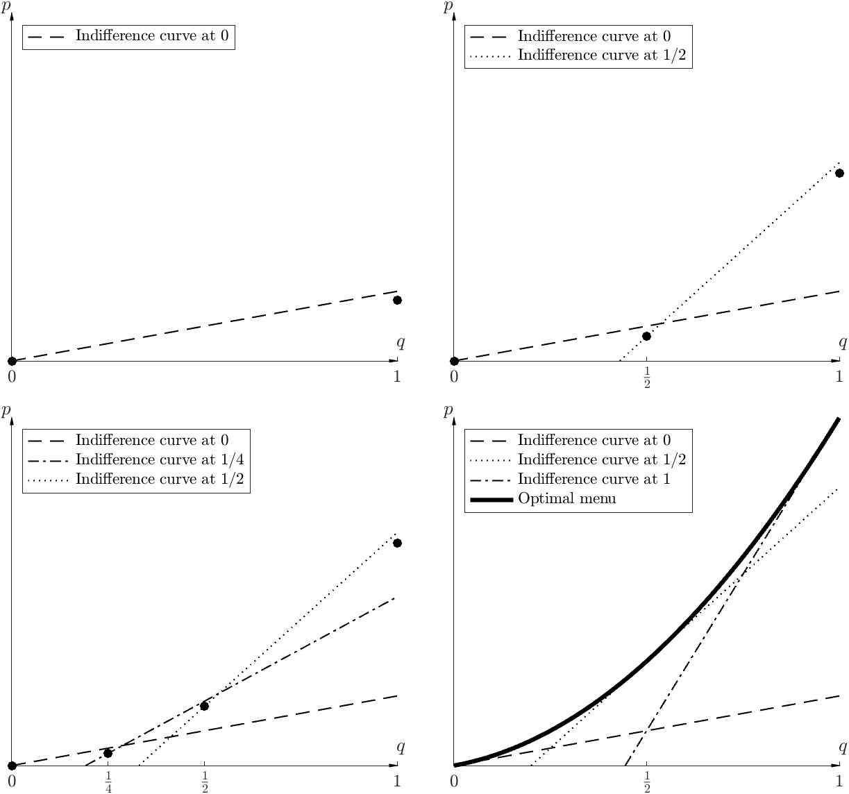
Figure 1: Improvement From $M_{2}$ (Upper Left) To $M_{3}$ (Upper Right),
$M_{4}$ (Lower Left), And $M^{*}_{\text{binary}}$ (Lower Right).

Two features are remarkable: (i) The new menu $M_{4}$ robustly induces full disclosure via local upward deviation, that is, every partial disclosure plan (including $(0,0)$) is broken by the next plan with a higher probability; (ii) The marginal price increment is upward bounded by the indifference curve of the high type at each plan to be broken. In particular, if $(q_{1},p_{1})$ and $(q_{2},p_{2})$ are adjacent plans with $q_{2}>q_{1}$, we must have bounded marginal price $\frac{p_{2}-p_{1}}{q_{2}-q_{1}}\leq\overline{\theta}-w^{N}(q_{1})$ where $w^{N}(q_{1})$ is the skepticism belief when the high type chooses $(q_{1},p_{1})$. These indifference curve slopes are interpreted as the high type’s marginal benefit of disclosure in different hypothetical equilibria as by disclosing marginally, the high type earns the type $\overline{\theta}$ and gives up the outside value $w^{N}(q_{1})$. As one can imagine, if we continue this improvement process, a continuous menu will emerge as a price function of disclosure probability, denoted by $p_{\text{binary}}^{*}(.)$, such that ${p_{\text{binary}}^{*}}^{\prime}(q)=\overline{\theta}-w^{N}(q)$ for all $q\in[0,1]$. The key to construction is to equate the marginal prices with their upper bounds, namely the slopes of indifference curves. In Figure 1, the lower right subfigure depicts three indifference curves that are tangent to the optimal price function. Formally, the optimal menu is approximated by (with small $\epsilon>0$):

$$M^{*}_{\text{binary}} =\{(q,p_{\text{binary}}^{*}(q)-\epsilon q):q\in[0,1]\}\text{, where}$$ (9)

$$p_{\text{binary}}^{*}(q) =\int_{0}^{q}\left[\overline{\theta}-w^{N}(\widetilde{q})\right]d\widetilde{q}=\int_{0}^{q}\left[\overline{\theta}-\frac{(1-\overline{\mu})\underline{\theta}+\overline{\mu}(1-\widetilde{q})\overline{\theta}}{(1-\overline{\mu})+\overline{\mu}(1-\widetilde{q})}\right]d\widetilde{q}=\int_{0}^{q}\frac{\overline{\theta}-\operatorname{\mathbb{E}}[\theta]}{1-\overline{\mu}\widetilde{q}}d\widetilde{q}$$

$$=-\frac{\overline{\theta}-\operatorname{\mathbb{E}}[\theta]}{\overline{\mu}}\ln(1-\overline{\mu}q).$$

Notice that in (9), the solution is written without replacing $\overline{\theta}$ or $\underline{\theta}$ with their values, and in interpreting our main result later in Section 4.1, we will invoke the form $p_{\text{binary}}^{*}(q)=-\frac{\overline{\theta}-\operatorname{\mathbb{E}}[\theta]}{\overline{\mu}}\ln(1-\overline{\mu}q)$.

The price $p_{\text{binary}}^{*}(.)$ is strictly convex and induces full disclosure in the unique equilibrium. Plugging in $\overline{\theta}=1$ and $\underline{\theta}=0$, we obtain $p^{*}_{\text{binary}}(q)=-\frac{1-\overline{\mu}}{\overline{\mu}}\ln(1-\overline{\mu}q)$. The platform’s maximal revenue guarantee is thus $\overline{\mu}p^{*}_{\text{binary}}(1)=-(1-\overline{\mu})\ln(1-\overline{\mu})$, strictly lower than full surplus $\overline{\mu}$.

Figure 2 depicts the maximal revenues under our worst-case implementation and the benchmark in Section 2.2 where best-case implementation was considered, and how they vary with the prior. The worst-case revenue curve is intuitive: the platform receives no revenue from quality disclosure when consumers are almost certain about the producer’s quality, whether good or bad. The platform’s profits are highest in the presence of significant uncertainty ($\overline{\mu}$ in the middle range).

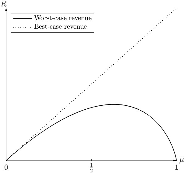
Figure 2: Revenue Under Worst-Case Implementation
And Best-Case Implementation

In contrast, the revenue curve for the best-case implementation seems problematic, as there is a sharp discontinuity at $\overline{\mu}=1$. In the corner case where the consumer is certain that the product has high quality, the platform will receive no revenue from the disclosure service, as there is nothing to disclose. However, as long as there is any small doubt so $\overline{\mu}<1$, the platform can extract all the surplus $\overline{\mu}$ away.

Discussion on bargaining power. The classical approach of assuming the principal can pick the favorite equilibrium is often justified by technique reasons, and in many classical settings, it is innocuous. However, when this assumption leads to significant differences, it becomes a questionable modeling choice, especially since it further strengthens the principal’s bargaining power in a context where the platform already has considerable bargaining leverage due to its ability to commit to a take-it-or-leave-it contract. To the extent that the bargaining position between the platform and the producer is perhaps not totally one-sided in reality and the classical principal-agent approach is sometimes a compromise to the lack of an ideal model of bargaining, we think that the worst-case equilibrium selection is an interesting reduce-form approach to give back some bargaining power to the producer.

4 Optimal Menu Profile

In this section, we establish our main result that provides the explicit forms of a robustly optimal menu profile and the maximal revenue guarantee. Section 4.1 states the main result, Theorem 1, followed by a discussion of its interpretation, implications, and proof sketch. Section 4.2 and Section 4.3 elaborate on each proof step and present three useful lemmas, through which we offer insights.

4.1 Main Result

Our main result finds that, to guarantee maximum revenue, the platform wants to robustly induce full disclosure by (i) offering a profile of continuous menus with strictly increasing marginal prices to break any under-advertising equilibrium with a local upward deviation of some type, and (ii) rationalizing the full disclosure choices of different types in a complete divide-and-conquer manner.

Specifically, the following menu profile robustly attains the maximal revenue guarantee:

Theorem 1.

There is a robustly optimal menu profile $M^{*\Theta}$ given by $M^{*K}=\{(0,0)\}$ and for all $k<K$:

$$M^{*k} =\{(q,p_{k}^{*}(q)):q\in[0,1]\}\text{, where }$$ (10)

$$p_{k}^{*}(q) =\frac{\theta^{k}-\operatorname{\mathbb{E}}[\theta|\theta\leq\theta^{k}]}{\Pr(\theta^{k}|\theta\leq\theta^{k})}\ln\frac{1}{1-\Pr(\theta^{k}|\theta\leq\theta^{k})q}.$$

Moreover, this profile induces a unique equilibrium where all types except $\theta^{K}$ choose the full disclosure plans while $\theta^{K}$ chooses zero disclosure. The maximal revenue guarantee is therefore $R^{*}=\sum_{k=1}^{K-1}\mu_{0}^{k}p_{k}^{*}(1)$.

To understand (10), recall that the optimal menu for the binary-type example offers the high type a strictly convex price function that breaks every hypothetical equilibrium where the high type discloses only partially by tempting her to deviate locally upward. The multiple-type solution (10) resembles the binary-type solution (9), which gives:

$$p_{\text{binary}}^{*}(q)=\frac{\overline{\theta}-\operatorname{\mathbb{E}}[\theta]}{\overline{\mu}}\ln\frac{1}{1-\overline{\mu}q}.$$

In this case, the high type is $\overline{\theta}$, the low type is $\underline{\theta}$, and $\overline{\theta}$ has prior probability $\overline{\mu}$.

By comparing (9) and (10), we find that the multiple-type optimal price, $p_{k}^{*}(.)$ for $k<K$, looks identical to the solution for a binary-type problem where the high type is $\overline{\theta}=\theta^{k}$ with prior $\overline{\mu}=\Pr(\theta^{k}|\theta\leq\theta^{k})$, and the low type is $\underline{\theta}=\operatorname{\mathbb{E}}[\theta|\theta<\theta^{k}]$. This is equivalent to excluding all types higher than $\theta^{k}$ from the problem and combining all types lower than $\theta^{k}$ to be the low type. Recall that in the binary-type case, the low type stays at zero disclosure, and the optimal menu equalizes the marginal prices to the high type’s marginal benefit of disclosure in different undesirable hypothetical equilibria. This, in (9), refers to ${p_{\text{binary}}^{*}}^{\prime}(q)=\overline{\theta}-w^{N}(q)$ for all $q\in[0,1]$, where $w^{N}(q)$ is the skepticism value when the high type discloses with probability $q$ (and low type with zero probability). This indicates that the optimal menu profile in Theorem 1 prices each type $\theta^{k}$ by also equalizing the marginal prices to the marginal benefit of disclosure in each hypothetical equilibrium where all types higher than $\theta^{k}$ fully disclose while all types lower than $\theta^{k}$ never disclose. Formally, the skepticism value $w^{N}(.)$ defined by (4) helps us to write the optimal marginal prices in Theorem 1 as the following, for all $k<K$ and $q\in[0,1]$:

$${p^{*}_{k}}^{\prime}(q)=\theta^{k}-w^{N}(\underbrace{1,...,1}_{k-1\text{ ones}},q,0,...,0)=\theta^{k}-w^{N}_{k}(q),$$ (11)

Where we use a shorthand notation $w^{N}_{k}(q)=w^{N}(1,...,1,q,0,...,0)$ with $k-1$ ones.

Complete divide-and-conquer. To interpret the price functions in Theorem 1 and their marginal prices given by (11), one can regard them as being constructed along a complete divide-and-conquer path. That is, the platform starts with the worst case where no type ever discloses. First, it increases the highest type $\theta^{1}$’s disclosure level to 1 while setting the marginal prices of $p_{1}^{*}(.)$ to equal the marginal benefit of disclosure at each level. This delivers (11) for $k=1$. Next, the platform turns to increasing the second highest type $\theta^{2}$’s disclosure level and pinning down $p_{2}^{*}(.)$ in a similar way, given that $\theta^{1}$ is already fully disclosing, which yields (11) for $k=2$. By iterating this procedure till the disclosure probability of the second lowest type $\theta^{K-1}$ is depleted, one obtains (11) and thus (10).

In other words, the platform adopts a complete divide-and-conquer strategy which sequentially and robustly induces full disclosure from $\theta^{1}$ to $\theta^{K-1}$. In particular, the platform offers $\theta^{1}$ a menu that breaks every hypothetical equilibrium where, regardless of all lower types’ behavior, $\theta^{1}$ discloses only partially. Given that full disclosure is the unique credible choice of $\theta^{1}$ that can appear in equilibrium, the platform offers $\theta^{2}$ a menu that breaks every hypothetical equilibrium where, regardless of all lower types’ behavior, $\theta^{1}$ discloses fully while $\theta^{2}$ discloses only partially. This procedure continues until full disclosure becomes the unique credible choice of $\theta^{K-1}$. It stops here because inducing disclosure out of the lowest type $\theta^{K}$ is never profitable as she would rather enjoy skepticism than paying anything for exposure.

We keep calling this divide-and-conquer strategy complete since the rationalization procedure above does not proceed in a partial and alternating manner. For example, the platform could have first robustly induced some disclosure level $q_{1}<1$ from $\theta^{1}$, then turned to $\theta^{2}$ for some level $q_{2}<1$, and come back to $\theta^{1}$ again for the remaining probability $1-q_{1}$. In fact, an important lemma discussed later, Lemma 2, implies that every menu profile corresponds to such a partial and alternating divide-and-conquer path such that the points on the path provide upper bounds for all marginal prices induced by the menus. For a loose formalization (which will be clear when we discuss Lemma 2), for all $k$ and $\widetilde{q}\in[0,1]$, there is a probability profile $q^{\Theta}$ on the path such that its $k$th component $q^{k}=\widetilde{q}$ and:

$$p_{k}^{\prime}(\widetilde{q})\leq\theta^{k}-w^{N}(q^{\Theta}),$$ (12)

Notice that (11) satisfies the complete divide-and-conquer version of (12). We say that a path that satisfies (12) has the property of pointwise upper-boundedness.

The assertion by Theorem 1 that complete divide-and-conquer outperforms all the alternating paths strikingly simplifies the solution form. To compare with literature, Segal (2003) (particularly his Lemma 3) suggests that with increasing externalities among players (or types in our case), alternating divide-and-conquer is usually optimal. In our setting, different types also have increasing externalities in the sense that by first inducing disclosure from high types, the consumer skepticism is worsened so that the other types’ disclosure becomes easier to induce. Moreover, the types are heterogeneous as the disclosure from a high type strikes down consumer skepticism more effectively than the “same” disclosure from a low type. Both observations above are consistent with the unraveling insight we gave when we discussed the binary-type example. We will see later how such monotonic-in-type increasing externalities form a crucial force that drives the complete divide-and-conquer solution.

Implications and simple implementation via volume-based pricing. Now, we discuss the implications we can make with Theorem 1 about advertisement pricing. First, despite the platform’s anticipation that the worst-case equilibrium will emerge, it manages to induce full disclosure. Full disclosure also happens in the classic disclosure setting studied by Grossman (1981) and Milgrom (1981) where the producer has free access to disclose its type. Nonetheless, the two settings clearly have different surplus allocations. The full disclosure feature of our solution depends on two things: (i) Advertising is costless, and (ii) the menu profile is type-dependent, so the platform can exploit the type information.

Second, each menu $M^{*k}$ (except for the lowest type) contains a continuum of plans, while only the full disclosure plan is chosen on the equilibrium path whereas most plans serve as baits, or carrots (in the terminology of Ali et al. (2022)) that induce local upward deviations for breaking all the under-advertising hypothetical equilibria. Such “dense” menus are useful in making the consumer believe that an equilibrium with any type partially disclosing cannot exist.

Third, denote the producer surplus conditional on each type $\theta^{k}$ by $W(\theta^{k})=\theta^{k}-p^{*}_{k}(1)$. Proposition 3 displays the main features of the producer’s surplus distribution across types. Since the platform needs to keep compensating the producer for giving up outside values, the surplus can be written as an interal $\int_{0}^{1}w_{k}^{N}(q)dq$. Moreover, the strategy of complete divide-and-conquer prioritizes attracting higher types into business by offering them better rents. This rent structure emerges even without an adverse selection issue, so it is not a result of incentive compatibility but instead stems from the platform’s optimal order of “conquering”. Namely, to induce disclosure from the highest type first, the platform keeps compensating her for giving up quite high outside values; however, once the highest type’s disclosure is guaranteed, the outside values are struck down, so the compensation to lower types will also be lower.

Proposition 3.

For all $k<K$, $W(\theta^{k})=\int_{0}^{1}w_{k}^{N}(q)dq$ and $\operatorname{\mathbb{E}}[\theta|\theta\leq\theta^{k}]>W(\theta^{k})>\operatorname{\mathbb{E}}[\theta|\theta\geq\theta^{k+1}]$. Thus, $W(\theta^{k})$ is strictly increasing in types.

However, being offered a higher rent does not mean the type would favor the presence of the platform since Proposition 3 also says that each type is strictly worse off than without the platform. To see this, notice that the upper bound $\operatorname{\mathbb{E}}[\theta|\theta\leq\theta_{k}]$ is strictly lower than both the type $\theta^{k}$ and the prior mean $\operatorname{\mathbb{E}}[\theta]$. These three numbers correspond to the respective surplus levels in three benchmarks: (i) If the platform is restricted to offering only bang-bang disclosure options, $W(\theta^{k})=\operatorname{\mathbb{E}}[\theta|\theta\leq\theta^{k}]$; (ii) If the platform is absent and the producer can self-advertise, $W(\theta^{k})=\theta^{k}$; (iii) If the platform is absent and the producer cannot self-advertise, $W(\theta^{k})=\operatorname{\mathbb{E}}[\theta]$. Hence, Proposition 3 shows that our platform extracts type-wise strictly higher surplus than in these benchmark setups.

To see Proposition 3, notice that according to (11), the price paid by type $\theta^{k}$ can be written as $p_{k}^{*}(1)=\int_{0}^{1}\left[\theta^{k}-w^{N}_{k}(q)\right]dq$. The type’s rent is therefore $\theta^{k}$ net this price, which becomes simply $\int_{0}^{1}w^{N}_{k}(q)dq$, the skepticism values accumulated along the path on which $\theta^{k}$’s disclosure is “conquered”. The rents are monotonic in types because the outside value $w_{k}^{N}(.)$ is strictly decreasing along the complete divide-and-conquer path. Furthermore, the outside value starts at the prior mean and eventually decreases to the lowest type. The rent is thus strictly lower than both the prior mean and the type.

One thing the reader might expect is that the price charged from a higher type should also be higher. Nonetheless, this is not true. For a counterexample, imagine three types with the two higher types being very close to each other and the middle type assigned with a very high prior. In this case, the price paid by the middle type will be higher than that of the highest type. The reason is that the type’s rent depends on the ability of her disclosure to strike down consumer skepticism, so a type with higher prior tends to face a lower rent and thus a higher price.

The last implication we make is that the optimal price functions in (10) take a logarithm form, indicating that once strategic uncertainty is accounted for, the platform has less tendency to adopt a linear pricing strategy such as per-click price. Instead, the classic rationale of Butters (1977) and Grossman and Shapiro (1984) for modeling volume-based pricing provides a class of convex price functions, remarkably similar to (10). We hence develop a simple implementation of our solution that (i) avoids the need for the platform to write contracts based on disclosure probability, which is hardly verifiable in practice, and (ii) makes concrete how the continuous menus can be implemented.

Specifically, the platform and the producer contract on the number of ad trials, $n$, and the associated prices $p_{n}$. This trial number indicates the volume of ads and $p_{n}$ is thus the volume-based prices. Given each trial, we assume the consumer sees the information with probability $\eta$, so with $n$ trials, the consumer is informed with probability $q=1-(1-\eta)^{n}$. In other words, to implement probability $q$, the platform needs to distribute $n(q)=\frac{\ln(1-q)}{\ln(1-\eta)}$ trials. If the platform charges a constant per-trial price, namely $p_{n}$ is linear in $n$, the relation between price and probability becomes $p(q)=p_{n(q)}=c\ln\frac{1}{1-q}$ for some $c>0$. This function resembles our solution (10) except that in the log-function of (10), we have an extra term $\Pr(\theta^{k}|\theta\leq\theta^{k})$. Such difference implies that we need nonlinear volume-based prices. For each $k<K$, the offer exclusive to type $\theta^{k}$ is:

$$p^{k}_{n}=-c^{k}\ln\left(1-\delta^{k}+\delta^{k}(1-\eta)^{n}\right),\text{ where }c^{k}=\frac{\theta^{k}-\operatorname{\mathbb{E}}[\theta|\theta\leq\theta^{k}]}{\Pr(\theta^{k}|\theta\leq\theta^{k})}\text{ and }\delta^{k}=\Pr(\theta^{k}|\theta\leq\theta^{k}).$$ (13)

This pricing strategy almost produces a constant per-trial price but with a distortion $\delta^{k}\in(0,1)$, and $p_{n}^{k}$ becomes linear in $n$ as $\delta^{k}\rightarrow 1$. Moreover, $p_{n}^{k}$ is strictly increasing and strictly concave in volume $n$, and it is bounded by $\lim_{n\rightarrow\infty}p_{n}^{k}=c^{k}\ln\frac{1}{1-\delta^{k}}$, so the per-trial price is decreasing and it eventually approximates zero. Thus, with such type-dependent volume-based prices, the platform induces a unique equilibrium where all types except for the lowest keep requesting more trials while the lowest never requests anything. Hence, the continuous menus in Theorem 1 are equivalent to diminishing per-trial prices in this sense. Besides, for another simple implementation, see Section 5.3 where we make equivalence between our solution and random pricing.

A sketch of proof. It is convoluted to show Theorem 1 because of the following challenge: In order to robustly induce a probability profile and maximize the revenue guarantee, the platform must “optimally” break every under-advertising hypothetical equilibrium with a deviation of some type; However, it faces two problems: (i) Which type of the producer deviates? and (ii) Which plan does the type deviate to? For binary-type cases, the answer to (i) is clearly the high type since it is never beneficial to offer the low type anything beyond the outside option. With additional arguments, the answer to (ii) is to always use local upward deviations. It is with these prerequisites that we can show (9) is optimal. In contrast, for multiple types, the answers to both (i) and (ii) are ambiguous because the equilibrium-breaking types and directions are now both within the platform’s discretion of choice.

Note that the pointwise upper-boundedness property (12) (see Lemma 2 for formal statement) provides a unifying answer to (ii) that we can always use local upward deviations to break equilibria. Building on this, the strategy of complete divide-and-conquer (see Lemma 3 for formal statement) answers (i) by suggesting the platform always uses the highest type that is not yet fully disclosing to break equilibria. Nonetheless, both claims are difficult to show.

We decompose the proof into four steps where the first three steps are supported by three lemmas, respectively, that will be discussed in Section 4.2 and Section 4.3. The four steps are:

Step 1 - We show that if a menu profile robustly induces a certain probability profile, it also does so if we lower-convexify each menu and delete all the plans that offer probabilities strictly higher than the robustly induced probability. We hence focus on such truncated convexifications.

Step 2 - We develop an algorithm that explicitly finds, for every menu profile, an alternating divide-and-conquer path that has the pointwise upper-boundedness property. To show the existence of such a path, we utilize the fact that every under-advertising probability profile cannot form an equilibrium. Further integration regarding both sides of the inequalities (12) yields an upper bound for the revenue guaranteed by the menu profile which we find the path for.

Step 3 - We show that the complete divide-and-conquer path gives such a revenue upper bound that is no less than any alternating divide-and-conquer path can provide. To show this, we explicitly construct an improvement for every alternating path by exchanging the order of “conquering” to let a high type’s disclosure probability be induced before that of a low type, and by continuing such improvement, we eventually obtain the complete divide-and-conquer path. Thus, the complete divide-and-conquer path determines an upper bound for the maximal revenue guarantee $R^{*}$.

Step 4 - We take a sequence of menu profiles $(M_{n}^{\Theta})_{n=1}^{\infty}$, where for all $n$ and $k<K$, $M_{n}^{k}=\{(q,p^{*}_{k}(q)-\frac{\epsilon}{n}q):q\in[0,1]\}$ where $\epsilon>0$ is small. This sequence converges to (10). We verify that every $M_{n}^{\Theta}$ induces full disclosure in the unique equilibrium and gives a revenue that approximates the upper bound for $R^{*}$ found in Step 3. So, $R^{*}$ equals this upper bound, and (10) gives a robustly optimal menu profile.

Once three more intermediate results are introduced in the following subsections, we will elaborate on insights for why it is optimal to adopt the complete divide-and-conquer strategy.

4.2 Pointwise Bounded Paths

The first step is to show it is without loss to focus on a subset of menu profiles, in which each profile (i) consists of lower-convexified menus, and (ii) robustly induces the plans with maximal probabilities.

To state the result, we define the price envelope of a menu $M$ which is denoted by $\check{p}_{M}:[0,Q_{M}]\rightarrow\mathbb{R}_{+}$ where $Q_{M}=\max\{q:(q,p)\in M\}$ is the maximal probability offered in $M$, The price envelope is defined as the highest convex function lying below the menu, given by $\check{p}_{M}(q)=\min\{p:(q,p)\in co(M)\}$ where $co(M)$ is the convex hull of $M$. We further call the graph of price envelope the (lower-)convexification of $M$, denoted as $\operatorname{conv}M$. This implies $\check{p}_{M}(.)$ has nondecreasing left- and right-derivatives at all interior points, denoted by $\check{p}_{M}(.-0)$ and $\check{p}_{M}(.+0)$, respectively. For simplicity, we sometimes denote by $p_{k}(.)$ the price envelope of menu $M^{k}$ when a menu profile $M^{\Theta}$ is specified in the context.

Lemma 1 says that if a menu profile $M^{\Theta}$ robustly induces some choice profile, it remains a worst-case equilibrium play even if, for every menu, we delete (i) all plans that lie above the convexification, and (ii) all plans that have higher probabilities than the robustly induced one. We call the resulting menu profile $\widehat{M}^{\Theta}$ defined in Lemma 1 the truncated convexification of $M^{\Theta}$, or sometimes convexified menus in short.

Lemma 1.

If a menu profile $M^{\Theta}$ robustly induces some contingent choices $\underline{r}^{\Theta}$, the menu profile $\widehat{M}^{\Theta}$ given by for all $k$, $\widehat{M}^{k}=\{(q,p)\in M^{k}\cap\operatorname{conv}M^{k}:q\leq\underline{q}^{k}\}$ also robustly induces $\underline{r}^{\Theta}$.

We prove Lemma 1 by first showing that we can focus on plans lying on the convexifications. To see this, note that for every contingent choice profile $(q^{\Theta},p^{\Theta})$, $\theta^{k}$’s indifference curve is $p(q)=p^{k}+(\theta^{k}-w^{N}(q^{\Theta}))(q-q^{k})$ and any plan that lies beneath this curve is a profitable deviation for her. This implies that: (i) $\theta^{k}$ reaches optimum if and only if the indifference curve is a subdifferential of the price envelope; (ii) If a profitable deviation exists, we can always find one on the price envelope. Therefore, it suffices to focus on convexifications for both verifying and breaking equilibria.

We then show that deleting high-probability plans is also harmless. This is less obvious since it could be that given $M^{\Theta}$, an under-advertising choice profile $(q^{\Theta},p^{\Theta})$ with $q^{\Theta}\leq\underline{q}^{\Theta}$ is broken by some type $\theta^{k}$ wanting to deviate upward to some $(q,p)\in M^{k}$ with $q>\underline{q}^{k}$, so deleting $(q,p)$ could cause problems. Let’s suppose this issue indeed creates an under-advertising equilibrium when the menu profile is $\widehat{M}^{\Theta}$. Fortunately, this cannot happen. The fact that indifference curves are subdifferentials of price envelopes in equilibrium implies that the indifference curve slopes in the under-advertising equilibrium are lower than in the equilibrium robustly induced by $M^{\Theta}$. This implies that if there is a deviation regarding the under-advertising profile given $M^{\Theta}$, it must be downward, instead of upward as supposed.

The second step for proving Theorem 1 is to show our central lemma that maps every menu profile to an alternating divide-and-conquer path that offers an upper bound for the revenue guaranteed by the menu profile. We define (and rename) an alternating divide-and-conquer path as follows:

Definition 3.

A nondecreasing alternating path from probability profile $\widetilde{q}_{1}^{\Theta}$ to profile $\widetilde{q}_{2}^{\Theta}$ with $\widetilde{q}_{1}^{\Theta}\leq\widetilde{q}_{2}^{\Theta}$ is a sequence of tuples $(q_{t}^{\Theta},k_{t})_{t=0}^{T}$ with $T$ being either finite or infinite. The path satisfies:

1. $q_{0}^{\Theta}=\widetilde{q}_{1}^{\Theta}$ and $\lim_{t\rightarrow T}q_{t}^{\Theta}=\widetilde{q}_{2}^{\Theta}$;

2. For all $t<T$, $q_{t}^{k_{t}}<q_{t+1}^{k_{t}}$ and $q_{t}^{-k_{t}}=q_{t+1}^{-k_{t}}$.

In other words, a nondecreasing alternating path specifies the step number $T$ and the moving direction $k_{t}$ for each step $t<T$, and the probability profile increases only its $k_{t}$th component in every step. We also call $k_{t}$ the direction type and the interval $[q_{t}^{k_{t}},q_{t+1}^{k_{t}}]$ the path stride of step $t$.

To illustrate what such a path looks like, we consider a three-type example. Let $\widetilde{q}_{1}^{\Theta}=0^{\Theta}$ and $\widetilde{q}_{2}^{3}=0$ as the lowest type will never disclose in equilibrium, so it suffices to consider moving in two directions. Figure 3 depicts a possible nondecreasing alternating path from $0^{\Theta}$ to $\widetilde{q}_{2}^{\Theta}$. In this case, the step number is $T=4$, and direction types are $k_{0}=k_{2}=1$ and $k_{1}=k_{3}=2$. The path is always nondecreasing as it moves by only increasing either $q^{1}$ or $q^{2}$ while holding the other directions unchanged.

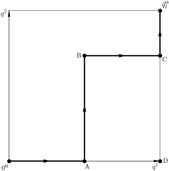
Figure 3: A Nondecreasing Alternating Path.

We now state the following important lemma:

Lemma 2.

If a menu profile $M^{\Theta}$ robustly induces some probability profile $\underline{q}^{\Theta}$, there exists a nondecreasing alternating path $(q^{\Theta}_{t},k_{t})_{t=0}^{T}$ from $0^{\Theta}$ to some $\widehat{q}^{\Theta}\leq\underline{q}^{\Theta}$ such that $R(M^{\Theta})$ is upward bounded by:

$$\sum_{t=0}^{T-1}\mu_{0}^{k_{t}}\int_{q^{k_{t}}_{t}}^{q^{k_{t}}_{t+1}}\left[\theta^{k_{t}}-w^{N}(\widetilde{q}^{k_{t}},q^{-k_{t}}_{t})\right]d\widetilde{q}^{k_{t}}.$$ (14)

In the proof of Lemma 2, we actually show a stronger version of the result which says that there is a pointwise upper bound for every marginal price, in the form of (12). In particular, each step $t$ has:

$$p_{k_{t}}^{\prime}(\widetilde{q})\leq\theta^{k_{t}}-w^{N}(\widetilde{q},q_{t}^{-k_{t}})\text{, for all }\widetilde{q}\in[q_{t}^{k_{t}},q_{t+1}^{k_{t}}].$$ (15)

In each step, the path increases the direction type who wants to deviate locally upward at each probability profile in the path stride where the other types’ probabilities stay still. Put differently, the left-hand side and the right-hand side of (15) represent the marginal cost and benefit of disclosure, respectively, for type $\theta^{k}$ in the hypothetical equilibrium where the probability profile is $(\widetilde{q},q_{t}^{-k_{t}})$. By integrating the left-hand side of (15) along the path weighted by prior probabilities, we can obtain the revenue in the worst-case equilibrium $R(M^{\Theta})$, so the integral with respect to the right-hand side of (15) produces an upper bound for the revenue guaranteed by the given menu profile.

The intuition Lemma 2 conveys is that every menu profile robustly induces a certain disclosure outcome as if it breaks all the under-advertising equilibria in an alternating manner with local upward deviations. Such alternating divide-and-conquer somewhat generalizes the complete divide-and-conquer feature of the robustly optimal menu profile.

Lemma 2, in a way, extends the necessary part of Lemma 3 by Segal (2003) to our setting who borrows the Round-Robin optimization procedure from Topkis (1998), Subsection 4.3.1. The difference, however, is significant. First, as mentioned when we discuss the binary-type example, producer types have indirect externalities, so the optimal menus tend to be continuous and the upper bounds (15) are rather pointwise than piecewise as in Segal’s Lemma 3(c). To see this, notice that an optimal deviation given one belief does not remain optimal with other beliefs, so we differ from Segal by using more than one plan in each path step. Second, Segal (2003) assumed increasing externalities, which our case does not have since if one induces probability out of a type lower than the skepticism value, it makes the other types harder to lure. This fact complicates the proof and invalidates a sufficient counterpart of Segal’s lemma.

The proof of Lemma 2 relies on an algorithm that explicitly finds a nondecreasing alternating path recursively. Our algorithm considers the following process: In every step $t$, as long as the path’s current location $q^{\Theta}$ has not reached the destination $\underline{q}^{\Theta}$, we find a type $\theta^{k}$ that wants to deviate upward, namely $p_{k}^{\prime}(q^{k})<\theta^{k}-w^{N}(q^{\Theta})$; We let $k$ be the new direction type and push the path toward this direction until it meets the first point where the upward-deviation inequality above fails; then, the next step begins. In this way, we guarantee (15) holds along the whole path. Notice that the criterion for upward deviation is expressed as a local condition, which is sufficient because the producer’s indifference curve is a straight line and the price envelop is convex.

An illustration is given by Figure 3. The path start at $0^{\Theta}$, where there must be some type that wants to deviate upward because, otherwise, $0^{\Theta}$ forms an under-advertising equilibrium. In Figure 3, the upward-deviating type is $\theta^{1}$. The path moves from $0^{\Theta}$ to point A by increasing the disclosure probability of $\theta^{1}$, and point A, associated with probability profile $q_{A}^{\Theta}$, is such that (i) upward deviation vanishes $p_{1}^{\prime}(q_{A}^{1}+0)\geq\theta^{1}-w^{N}(q_{A}^{\Theta})$, and (ii) for all $q^{\Theta}$ lying between $0^{\Theta}$ and A, upward deviation exists $p_{1}^{\prime}(q^{1}+0)<\theta^{1}-w^{N}(q^{\Theta})$. With a continuity argument, (ii) implies $p_{1}^{\prime}(q^{1}_{A}-0)\leq\theta^{1}-w^{N}(q_{A}^{\Theta})$. This along with (i) implies that if $(q_{A}^{1},p_{1}(q_{A}^{1}))$ is contained in $M^{1}$, then by choosing this plan, $\theta^{1}$ reaches its optimum given the skepticism belief at point A. $M^{1}$ indeed must have offered this plan because (ii) implies that $\theta^{1}$ has been greater than the skepticism value on the path stride from $0^{\Theta}$ to A, so further increasing her disclosure level can only worsen skepticism. We then show that if there is no plan offered at A, then the marginal price envelope is locally constant, and (i) and (ii) cannot coexist. Thus, to prevent $q_{A}^{\Theta}$ from forming an under-advertising equilibrium, $\theta^{2}$ must want to deviate upward at A.

So, the path moves from A to point B by increasing the disclosure level of $\theta^{2}$, and point B is the first point for $\theta^{2}$’s upward-deviation inequality to fail. Repeating previous arguments, we show that $\theta^{2}$ reaches its optimum there. Since B cannot form an equilibrium, $\theta^{1}$ must want to deviate at this point. Suppose $\theta^{1}$ wants to deviate downward. We adopt an argument that is somewhat related to Round-Robin (see Segal (2003), Lemma 3) to obtain a contradiction. Notice that $\theta^{2}$’s willingness to deviate upward at A requires her type to be greater than the skepticism value there, so increasing her disclosure level can only worsen the skepticism further. Hence, if $\theta^{1}$ is not afraid of consumer’s skepticism at B and thus wants to deviate downward, then she also cannot be afraid of the skepticism at A, contradicting her optimality at A. This means she must want to deviate upward at B.

So, the path moves from B to point C where $\theta^{1}$ depletes its probability. With similar logic, we show $\theta^{2}$ must want to deviate upward at C, and thus the path moves up again and ends at its destination $\widetilde{q}_{2}^{\Theta}$.

Two things worth mentioning about the general proof of Lemma 2 are: (i) When the path arrives at a point like C in Figure 3, Lemma 1 which allows us to ignore all plans with excessive probabilities is significant in eliminating the possibility that the hypothetical equilibrium here is broken by the upward deviation of $\theta^{1}$, who has reached her induced probability; (ii) The algorithm must end within countable steps since, otherwise, we can show that the path converges to a point that forms an under-advertising equilibrium using arguments related to those in the above illustration.

4.3 An Upper Bound for Maximal Revenue Guarantee

We have shown that the revenue guarantee of every menu profile is controlled by an upper bound determined by a nondecreasing alternating path. Each such path has a fixed starting point $0^{\Theta}$ and a flexible endpoint $\underline{q}^{\Theta}\leq 1^{\Theta}$. To further bound the maximal revenue guarantee $R^{*}$, we search among all such paths to maximize the path-specific bound (14).

The following result states that the complete divide-and-conquer path is optimal:

Lemma 3.

The bound (14) is maximized by the full disclosure profile $\underline{q}^{\Theta}=(1,...,1,0)$ and the complete divide-and-conquer path $(q_{t}^{\Theta},k_{t})_{t=0}^{K-1}$ where for all $t<K-1$, $k_{t}=t+1$ and $q_{t}^{\Theta}=(1,...,1,0,...,0)$ with $t$ ones. Moreover, the maximal value of (14) puts an upper bound for $R^{*}$, which is:

$$\sum_{k=1}^{K-1}\mu_{0}^{k}\frac{\theta^{k}-\operatorname{\mathbb{E}}[\theta|\theta\leq\theta^{k}]}{\Pr(\theta^{k}|\theta\leq\theta^{k})}\ln\frac{1}{1-\Pr(\theta^{k}|\theta\leq\theta^{k})}.$$ (16)

For the example in Figure 3, the complete divide-and-conquer path corresponds to moving the path first along the bottom edge and then up along the right edge, namely from $0^{\Theta}$ to point D to $\widetilde{q}_{2}^{\Theta}$.

The insight for the optimality of the complete divide-and-conquer path is related to the intuition we gave in the binary-type example: More disclosure out of high types worsens consumer skepticism, which is also the opportunity cost of nondisclosure, “faster” than inducing disclosure from low types.

To see this formally, consider finding the optimal path while fixing the endpoint to be the full disclosure profile $(1,...,1)$. We use a quantile $Q\in[0,1]$ to parameterize each path $(q_{t}^{\Theta},k_{t})_{t=1}^{T}$. That is, for every $Q$, find the step $t^{\prime}$ such that:

$$\underline{Q}_{t^{\prime}}:=\sum_{t=0}^{t^{\prime}-1}\mu^{k_{t}}_{0}(q_{t+1}^{k_{t}}-q_{t}^{k_{t}})\leq Q\leq\overline{Q}_{t^{\prime}}:=\sum_{t=0}^{t^{\prime}}\mu^{k_{t}}_{0}(q_{t+1}^{k_{t}}-q_{t}^{k_{t}}).$$ (17)

Let $t^{\prime}$ vary with $Q$ as above, and redenote the path by:

$$q^{\Theta}_{Q}=(q^{k_{t^{\prime}}}_{t^{\prime}}+(Q-\underline{Q}_{t^{\prime}})/\mu^{k_{t^{\prime}}}_{0},q^{-k_{t^{\prime}}}_{t^{\prime}})\text{, for all }Q\in[0,1].$$ (18)

In other words, $Q$ denotes the total ex-ante probability that has already been robustly induced along the path. $t^{\prime}$ represents the path step in which $Q$ is reached, and $q_{Q}^{\Theta}$ marks the position by which the path has induced total probability $Q$. The bound (14) can be rewritten as:

$$\sum_{t=0}^{T-1}\mu_{0}^{k_{t}}\int_{q^{k_{t}}_{t}}^{q^{k_{t}}_{t+1}} \left[\theta^{k_{t}}-w^{N}(\widetilde{q}^{k_{t}},q^{-k_{t}}_{t})\right]d\widetilde{q}^{k_{t}}$$ (19)

$$=\sum_{t=0}^{T-1}\mu_{0}^{k_{t}}\int_{q^{k_{t}}_{t}}^{q^{k_{t}}_{t+1}}\theta^{k_{t}}d\widetilde{q}^{k_{t}}-\sum_{t=0}^{T-1}\mu_{0}^{k_{t}}\int_{q^{k_{t}}_{t}}^{q^{k_{t}}_{t+1}}w^{N}(\widetilde{q}^{k_{t}},q^{-k_{t}}_{t})d\widetilde{q}^{k_{t}}$$

$$=\operatorname{\mathbb{E}}[\theta]-\sum_{t=0}^{T-1}\int_{\underline{Q}_{t}}^{\overline{Q}_{t}}w^{N}(q_{Q}^{\Theta})dQ$$

$$=\operatorname{\mathbb{E}}[\theta]-\int_{0}^{1}w^{N}(q_{Q}^{\Theta})dQ.$$

We thus decompose it into two simple parts, $\operatorname{\mathbb{E}}[\theta]$ and $\int_{0}^{1}w^{N}(q_{Q}^{\Theta})dQ$. Only the latter is path-specific and determined by how consumer skepticism changes along the path. This new form expresses the previous insight formally: No matter whether a type is high or low, its disclosure will be induced sooner or later, which results in the non-path-specific constant $\operatorname{\mathbb{E}}[\theta]$; An optimal path constructs a mapping $q_{Q}^{\Theta}$ that drives the skepticism value down as “fast” as possible to minimize the total compensation to the producer for giving up outside values along the path, which equals $\int_{0}^{1}w^{N}(q_{Q}^{\Theta})dQ$; The most effective strategy is to prioritize the highest type whose probability has not yet been depleted.

The proof of Lemma 3 follows the same logic. In particular, for every path that is not complete divide-and-conquer, we can always find two consecutive steps where the direction type of the first step is lower than that of the second step. We show that by exchanging the order of these steps, the path ends up with a higher value of (14). All paths can be improved with a sequence of such exchanges until they become (or approximate) complete divide-and-conquer.

Again, we use Figure 3 as an illustration. The plotted path can be improved by exchanging the moving directions of its second and third steps, which leads to the complete divide-and-conquer path. To exhibit the improvement graphically, for every path $q_{Q}^{\Theta}$, define its quantile-skepticism value $w^{N}(Q):=w^{N}(q_{Q}^{\Theta})$. Then, (19) says that a better path must yield a smaller integral $\int_{0}^{1}w^{N}(Q)dQ$, namely a smaller area below its quantile-skepticism value. Figure 4 depicts the quantile-skepticism values associated with the original path and the improved path in Figure 3 that we described. We mark in Figure 4 the correspondences of points A, B, C, and D. The original path moves along A-B-C whereas the improved path passes A-D-C.

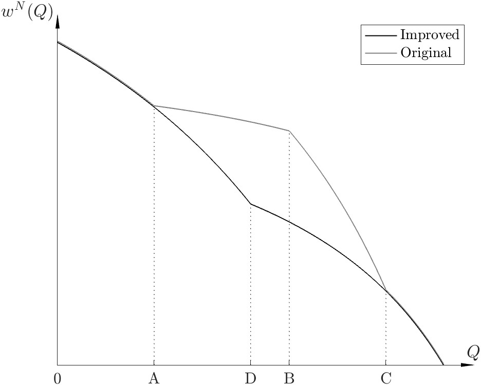
Figure 4: Quantile-Skepticism Values Of Two Paths.

As one can see in Figure 4, the quantile-skepticism value of the improved path is uniformly no greater than that of the original path with the middle part from A to C being strictly lower. We have segments satisfying AD=BC and AB=DC, meaning the exchange of two steps does not affect the total probabilities induced out of each type. Nonetheless, the skepticism value drops faster on AD than on AB because the improved path induces the highest type’s disclosure first. Also, the skepticism value drops faster on DC than on AB, both of which correspond to the revelation of the lower type. This feature results from the fact that the types have increasing externalities, that is to say, more disclosure from a higher type makes it easier to induce disclosure from a lower type.

With this optimal path, we obtain an upper bound (16) for $R^{*}$. By comparing (16) and (10), one can see that this bound is exactly the full disclosure revenue $\sum_{k=1}^{K-1}\mu^{k}_{0}p_{k}^{*}(1)$ given by the solution claimed in Theorem 1. Consequently, the only thing left is to show that this claimed menu profile indeed guarantees full disclosure in the worst-case equilibrium, which we relegate to the Appendix.

5 Extensions

We now discuss four extensions. Section 5.1 shows that the unique equilibrium induced by the robustly optimal menu profile can also be solved with iterated deletion of strictly dominated strategies. Thus, our solution is robust under weaker assumptions on player behavior. Section 5.2 analyzes the platform that can jointly design the information structure and the menu profile. We show that the platform wants to perfectly reveal the types, based on which we compare our model with that of Ali et al. (2022). Section 5.3 allows the platform to offer random menus (in the sense of Halac et al. (2021)). We show that it suffices to consider nonrandom menus for achieving maximal revenue guarantee, whereas a class of random menus is equivalent to the robustly optimal menu profile and takes the form of bang-bang menus with price dispersion. Section 5.4 shows that the two main features of our solution are preserved even with costly advertising.

5.1 Rationalizable Outcomes

Traditionally, the term strategic uncertainty may refer to multiple equilibria as well as multiple rationalizable outcomes. This subsection shows that choosing different concepts does not matter: The menu profile in Theorem 1 remains robustly optimal even if the platform seeks to maximize revenue guarantee among all rationalizable outcomes.

In Section 2.1, we show that the disclosure game induced by a menu profile simply consists of the producer’s contingent choices of ad plans $r^{\Theta}$ and the consumer’s skepticism belief $\mu^{N}$. The implicit modelling of the consumer’s strategy is that the consumer decides whether to purchase the product or not, when facing the take-or-leave-it offer from the producer. Thus, the consumer’s formal strategy is a mapping $a:(\Theta\cup N)\times\mathbb{R}\to\{0,1\}$, where $a=1$ means the consumer purchases the product. In any equilibrium of the producer-consumer game, the consumer’s strategy takes the following form:

$$\begin{cases}a(\theta,p)&=1_{\theta\geq p},\quad\forall\theta,\\ a(N,p)&=1_{w^{N}\geq p}.\end{cases}$$

Here, $w^{N}$ is the consumer’s skepticism value defined by (4). Note that this class of strategy is parameterized by a single variable $w^{N}$, so we denote this strategy as $a^{w^{N}}$.

With this extended model, in this subsection we consider the simultaneous move game between the producer and the consumer, where the consumer’s strategy is a function $a$ defined above and producer’s strategy $r^{\Theta}$ maps her types to a (potentially mixed) choice of ad plan. Both parties choose their strategy to maximize their ex-ante expected utility. According to the Harsanyi transformation, the Nash equilibrium of this game is also the equilibrium in our main specification. The purpose of this subsection is to show that the optimal menu profile in Theorem 1 also induces a unique rationalizable outcome in this producer-consumer simultaneous move game.

First, notice that for any producer strategy $r^{\Theta}$, the consumer’s best response is exactly the strategy $a^{w^{N}}$ with $w^{N}=\operatorname{\mathbb{E}}_{\mu^{N}}[\theta]$ where $\mu^{N}$ follows the Bayes rule (2) given $r^{\Theta}$. This means any consumer strategy $a$ that does not take the form of $a^{w}$ cannot be the best response to any strategy of the producer. Therefore, to discuss rationalizable outcomes, the set of consumer strategies that we need to consider is $\{a^{w}:w\in[\theta^{K},\theta^{1}]\}$ where $\theta^{K}$ and $\theta^{1}$ respectively specify the lower and upper bounds of a skepticism value. We identify the strategy $a^{w}$ simply with the threshold $w$. Formally, given a menu profile $M^{\Theta}$, we define:

$$\Sigma^{P}_{0}:=\{r^{\Theta}:r^{k}\in M^{k}\text{ for all }k\};\qquad\Sigma^{C}_{0}:=[\theta^{K},\theta^{1}].$$ (20)

These two sets are the “strategy space” of the producer and the consumer in a simultaneous move game. Also, we let $u(r^{\Theta},w^{N})=\sum_{k=1}^{K}q^{k}\theta^{k}+(1-q^{k})w^{N}-p^{k}$ denote the producer’s utility function.

Definition 4.

The process of iterated deletion of strictly dominated strategies proceeds as follows. For $n\geq 1$, define $\Sigma_{n}^{P}$ and $\Sigma_{n}^{C}$ recursively by:

$$\Sigma_{n}^{P} =\{r^{\Theta}\in\Sigma^{P}_{n-1}:\text{there is no }\widetilde{r}^{\Theta}\in\Sigma^{P}_{n-1}\text{ such that }u(\widetilde{r}^{\Theta},w^{N})>u(r^{\Theta},w^{N})\text{ for all }w^{N}\in\Sigma^{C}_{n-1}\};$$ (21)

$$\Sigma_{n}^{C} =\{w^{N}\in\Sigma^{C}_{n-1}:w^{N}=\operatorname{\mathbb{E}}_{\mu^{N}}[\theta]\text{ where $\mu^{N}$ follows the Bayes rule (\ref{bayes}) given some }r^{\Theta}\in\Sigma^{P}_{n-1}\}.$$

Define $\Sigma_{\infty}^{P}=\cap_{n=0}^{\infty}\Sigma_{n}^{P}$ and $\Sigma_{\infty}^{C}=\cap_{n=0}^{\infty}\Sigma_{n}^{C}$. These are the sets of producer and consumer strategies that survive the iterated deletion of strictly dominated strategies.

Since the robustly optimal menu profile $M^{*\Theta}$ given by Theorem 1 is defined as the limit of a sequence of profiles, to deal with strict dominance, we define (for small $\epsilon>0$) the $\epsilon$-optimal menu profile $M^{*\Theta}_{\epsilon}$ by: For all $k$, $M^{*\Theta}_{\epsilon}=\{(q,p-\epsilon q):(q,p)\in M^{*\Theta}\}$. In other words, we focus on the approximating sequence where the prices are slightly lower than in the optimal solution. The following proposition establishes that given the $\epsilon$-optimal menu profile, the survivors of iterated strict dominance are given by the unique equilibrium induced by the menu profile:

Proposition 4.

Given $M^{*\Theta}_{\epsilon}$, $\Sigma^{P}_{\infty}$ contains a single strategy of all types fully disclosing except for the lowest type, and $\Sigma^{C}_{\infty}$ contains a single value of the lowest type.

By definition, the maximal revenue guarantee among all equilibria naturally serves as an upper bound on the revenue guarantee among all rationalizable outcomes. Now that Proposition 4 demonstrates the menu profile achieves this upper bound by inducing a unique rationalizable outcome, our menu profile remains optimal under a different robust criterion.

We prove Proposition 4 in three steps. First, we show in the first round of deletion, all non-monotonic producer strategies are strictly dominated. In particular, we take any such strategy $r^{\Theta}$ and assume there are two types $\theta^{k_{1}}>\theta^{k_{2}}$ whose probabilities have $q^{k_{1}}<q^{k_{2}}$. We then construct a different strategy by increasing $q^{k_{1}}$ to $\widetilde{q}^{k_{1}}$ and decreasing $q^{k_{2}}$ to $\widetilde{q}^{k_{2}}$ while preserving the total ex-ante probability $\mu_{0}^{k_{1}}q^{k_{1}}+\mu_{0}^{k_{2}}q^{k_{2}}=\mu_{0}^{k_{1}}\widetilde{q}^{k_{1}}+\mu_{0}^{k_{2}}\widetilde{q}^{k_{2}}$. Irrespective of consumer skepticism values, the new strategy gives a higher payoff than the original one does. Second, the fact that only monotonic producer strategies can survive the first round implies that only the skepticism values no less than the prior mean can survive the second round. Last, in the third round, any producer strategy with the highest type choosing a probability lower than some small $\delta_{1}$ cannot survive because the construction of her menu $M^{*1}$ induces local upward deviation as long as the skepticism values are no greater than the prior mean. Thus, in the fourth round, the surviving skepticism values must be “lower” than in the previous round because the highest type now at least discloses with probability $\delta_{1}>0$. Given this, then in the fifth round, the construction of $M^{*1}$ further deletes the strategies where the highest type chooses a probability lower than $\delta_{1}+\delta_{2}$ with some small $\delta_{2}>0$. And one can imagine how this leads to the complete deletion of all strategies where the highest type chooses partial disclosure. Recalling the complete divide-and-conquer construction of $M^{*\Theta}$, one can further imagine how such complete deletion will continue until the second lowest type.

5.2 Joint Design of Evidence Structure

The main model makes an important assumption that the platform obtains a hard evidence of the product’s value, which could be, e.g., a certificate generated by a test. It is sometimes possible that the platform can also control the testing process. We consider the platform’s joint design of information structure and price profile. This extension helps to compare our setting with Ali et al. (2022) who consider an information design problem with pricing on disclosure opportunities.

Changing the language a bit, we have states $\theta^{1}\geq\theta^{2}\geq...\geq\theta^{K}\in\Theta$ with a prior belief $\mu_{0}=(\mu^{k}_{0})_{k=1}^{K}$. A signal (or an information structure) is a profile of conditional distributions $\pi:\Theta\rightarrow\Delta(S)$ where $S$ is a space of signal realization and $\Delta(S)$ denotes the space of probability distributions over $S$. We consider signals fully supported by finite realizations, namely $|S|<\infty$.

The signal realizations correspond to the types in the main model, being the verifiable objects that the platform can contract on and the consumer will believe.

Here is the timing. First, the platform, only knowing the prior, publicly chooses both a signal and a realization-specific menu profile, denoted by $M^{S}=(M^{s})_{s\in S}$. The signal realizes and both the platform and the producer observe the realization, say $\widetilde{s}$, and then the producer chooses a plan from $M^{\widetilde{s}}$. Then, disclosure, price payment, belief updating, and trading happen accordingly as in the main model.

Let $\mathcal{S}$ collect all the finite realization spaces, and given a realization space $S$, $\Pi(S)$ and $\mathcal{M}(S)$ collect all the signals and menu profiles, respectively. The platform’s objective is to choose a signal that admits a robustly optimal menu profile that achieves the following jointly maximal revenue guarantee:

$$R^{**}=\sup_{S\in\mathcal{S}}\sup_{\pi\in\Pi(S)}\left[\sup_{M^{S}\in\mathcal{M}(S)}\inf_{g\in\mathcal{E}(M^{S})}\sum_{s\in S}\sum_{k=1}^{K}\mu^{k}_{0}\pi(s|\theta^{k})p^{s}\right].$$ (22)

The following result states that the optimal information structure is perfectly revealing:

Proposition 5.

With $S=\Theta$ and the perfectly revealing signal, (10) gives a robustly optimal menu profile that achieves $R^{**}$. Moreover, $R^{**}=R^{*}$.

Proposition 5 shows that the platform dislikes noisy signals and every bit of informativeness can be profitable. This result, however, contrasts the solution given by Ali et al. (2022) who study a noisy and continuous signal. The main cause of this difference is that their setting does not allow for commitment to type-dependent menus or partial disclosure plans. Instead, they consider a disclosure fee uniform across all types. We hence suggest that once the platform has great pricing power, it wants the informational details to be rather straightforward.

The intuition behind Proposition 5 is that since the platform’s goal, given by (19), is to strike down consumer skepticism as “fast” as possible, it desires the posterior distribution the signal induces to be as segregated as possible. To offer a formal understanding, we first show in the proof that, given a signal $\pi$, the choice of menu profile is equivalent to the same choice in the main model where the types are essentially the posterior means, namely for all $s\in S$:

$$\text{posterior }\mu^{s}:\theta^{k}\mapsto\frac{\mu^{k}_{0}\pi(s|\theta^{k})}{\sum_{j=1}^{K}\mu^{j}_{0}\pi(s|\theta^{j})},\text{ posterior mean }\widetilde{\theta}^{s}=\operatorname{\mathbb{E}}_{\mu^{s}}[\theta].$$ (23)

By abusing the notations a bit, we reorder and rename the types as $\widetilde{\theta}^{1}\geq\widetilde{\theta}^{2}\geq...\geq\widetilde{\theta}^{|S|}$. In addition, the signal and the prior together induce a distribution of these types, denoted by $(\widetilde{\mu}^{k}_{0})_{k=1}^{|S|}$, which also forms a posterior distribution $\tau$ that must satisfy the Bayes plausibility condition $\operatorname{\mathbb{E}}_{\tau}[\mu^{s}]=\mu_{0}$ (e.g., Kamenica and Gentzkow (2011)). This implies $\operatorname{\mathbb{E}}[\widetilde{\theta}]=\operatorname{\mathbb{E}}_{\tau}\left[\sum_{k=1}^{K}\mu^{s}(\theta^{k})\theta^{k}\right]=\sum_{k=1}^{K}\mu^{k}_{0}\theta^{k}=\operatorname{\mathbb{E}}[\theta]$. Thus, the first part of (19) is pinned down regardless of the signal, so the optimal signal seeks to minimize the second part regarding the quantile-skepticism value $w^{N}(.)$.

Given each signal, Theorem 1 allows us to focus on the menu profile that induces full disclosure via complete divide-and-conquer, which maps every signal to a well-defined quantile-skepticism value. As one may anticipate, the perfectly revealing signal and the complete divide-and-conquer strategy prioritize inducing disclosure from the highest possible type $\widetilde{\theta}^{1}=\theta^{1}$, ensuring $w^{N}(.)$ is the lowest possible for all $Q\leq\mu^{1}_{0}$. Similar arguments continue as once the first $\mu^{1}_{0}$ probability is depleted, the current highest type $\widetilde{\theta}^{2}=\theta^{2}$ becomes the next target. Sequentially, we conclude that the perfectly revealing signal induces a quantile-skepticism value that is pointwise no greater than any other signal would do.

5.3 Random Menus

As pointed out by Halac et al. (2021), introducing uncertainty in menu offers can reduce the principal’s cost of ensuring efforts from multiple agents. This section illustrates that, in our framework, introducing random menus does not help improve the platform’s revenue guarantee. On the other hand, allowing for random menus helps us to provide a different implementation of the robustly optimal menu profile in Theorem 1, where the platform simply offers a type-dependent random price for full disclosure. This implementation is more practical in settings where the platform cannot commit to partial disclosure, such as the credit agency in Ali et al. (2022).

By introducing uncertainty in menu offers, we refer to the following setup. The platform still chooses a profile of type-dependent menus but with each menu being potentially stochastic. In particular, let $\mathcal{M}^{k}$ be the set of all deterministic menus of the form (1), and $\Delta(\mathcal{M}^{k})$ collects all the probability distributions over deterministic menus. The platform now chooses a random menu profile $\widetilde{M}^{\Theta}=(\widetilde{M}^{k})_{k=1}^{K}$ where for all $k$, $\widetilde{M}^{k}\in\Delta(\mathcal{M}^{k})$. We call a random menu profile deterministic if for all $k$, $\widetilde{M}^{k}$ is supported by a single deterministic menu, and we also refer to $\widetilde{M}^{k}$ as its deterministic support. Finally, given a random menu $\widetilde{M}$, let $\operatorname{\mathbb{E}}_{M\sim\widetilde{M}}[.]$ denote the expectation regarding the distribution $\widetilde{M}$ and $M$ is a typical realization.

Here is the timing. First, the platform publicly chooses a random menu profile. After this, importantly, both the type $\theta^{k}$ and a deterministic menu $M^{k}$ are realized according to the type-dependent distribution $\widetilde{M}^{k}$. The producer picks a plan from the realized menu. Next, disclosure, price payment, belief updating, and trading happen accordingly. Both the platform and the producer observe everything while the consumer cannot observe the type, the realized menu, or the producer’s choice.

Given a random menu profile, a disclosure equilibrium consists of the producer’s choices contingent on both type and menu realizations, and the consumer’s skepticism belief. We say two disclosure equilibria (potentially induced by different menu profiles) are outcome-equivalent if (i) they have the same skepticism belief, and (ii) conditional on each type, they induce identical platform and producer expected payoffs. We say two random menu profiles are outcome-equivalent if, for every equilibrium induced by either profile, there is an outcome-equivalent equilibrium induced by the other profile. We establish that every random menu profile is outcome-equivalent to a deterministic menu profile:

Proposition 6.

For every random menu profile $\widetilde{M}^{\Theta}$, an outcome-equivalent deterministic menu profile $M^{\Theta}$ is given by for all $k$, $(q,p)\in M^{k}$ if and only if there are $w\in[\theta^{K},\theta^{1}]$ and random variables $q_{M}^{k}$ and $p_{M}^{k}$ such that $q=\operatorname{\mathbb{E}}_{M\sim\widetilde{M}^{k}}[q^{k}_{M}]$, $p=\operatorname{\mathbb{E}}_{M\sim\widetilde{M}^{k}}[p^{k}_{M}]$, and $(q^{k}_{M},p^{k}_{M})\in\arg\max_{(q^{\prime},p^{\prime})\in M}q^{\prime}\theta^{k}+(1-q^{\prime})w-p^{\prime}$.

In words, the above outcome-equivalent deterministic menu profile is constructed by adding all pairs of expected optimal probability and expected optimal price under any possible skepticism value, given the random menu profile. The key to such equivalence is the fact that only the type-dependent expected disclosure probabilities matter when the Bayes rule yields the skepticism belief.

An immediate implication of Proposition 6 is that it suffices to implement the maximal revenue guarantee with merely deterministic menu profiles as in the main model.

However, allowing for random menus enriches the possible forms of robustly optimal menu profiles. In particular, the platform faces a realistic concern that it sometimes cannot commit to partial disclosure whereas random price offers are more accessible. For example, the platform cannot perfectly control how information is disseminated among consumers, nor can it precisely determine the proportion of informed consumers. We thus consider the bang-bang menus with price dispersion, namely random menus that are supported by deterministic menus offering only full disclosure plans.

The following delivers a robustly optimal profile of bang-bang menus with price dispersion:

Proposition 7.

A robustly optimal random menu profile $\widetilde{M}^{*\Theta}$ is given by $\widetilde{M}^{*K}=\{(0,0)\}$ and for all $k<K$, $\widetilde{M}^{*k}$ is supported by deterministic menus $M^{k}_{p}=\{(0,0),(1,p)\}$ for all $p\in[{p_{k}^{*}}^{\prime}(0),{p_{k}^{*}}^{\prime}(1)]$ and $\widetilde{M}^{*k}$ induces the cumulative distribution function of price $p$ given by $H^{k}(p)=({p_{k}^{*}}^{\prime})^{-1}(p)$.

Proposition 7 is an immediate corollary of Proposition 6 which gives $M^{*\Theta}$ as the outcome-equivalent deterministic menu profile of $\widetilde{M}^{*\Theta}$. To offer an example of such price dispersion, consider the binary type example discussed in Section 3, and the associated optimal random menu for the high type is represented by the following price distribution:

$$H_{\text{binary}}(p)=\frac{1}{\overline{\mu}}\left(1-\frac{\overline{\theta}-\operatorname{\mathbb{E}}[\theta]}{p}\right)\text{, for all }p\in\left[\overline{\theta}-\operatorname{\mathbb{E}}[\theta],\overline{\theta}-\underline{\theta}\right].$$ (24)

Observe that without accounting for strategic uncertainty as in our benchmark (Section 2.2), the platform offers the high type a single plan $(1,\overline{\theta}-\underline{\theta})$. Comparing this with $H_{\text{binary}}(.)$, we learn that taking into consideration strategic uncertainty gives rise to downward price dispersion since $\overline{\theta}-\operatorname{\mathbb{E}}[\theta]<\overline{\theta}-\underline{\theta}$.

5.4 Advertising Costs

Our analysis assumed that advertising is costless for the platform, which, however, may not be a good approximation of the reality. Suppose the platform incurs a cost $c(q)$ when implementing a plan with disclosure probability $q\in[0,1]$. We do not impose too much structure on the costs except that $c(.)$ is nonnegative and continuous. We now turn to the maximal profit guarantee:

$$P^{*}:=\sup_{M^{\Theta}\in\mathcal{M}}\inf_{g\in\mathcal{E}(M^{\Theta})}\sum_{k=1}^{K}\mu_{0}^{k}(p^{k}-c(q^{k})).$$ (25)

The following result shows that most features of our main result hold but the robustly induced disclosure outcome now could be partial disclosure:

Proposition 8.

There is some probability profile $q^{*\Theta}$, and a robustly optimal menu profile $M^{*\Theta}$ given by, for all $k<K$:

$$M^{*k} =\{(q,\widetilde{p}_{k}(q)):q\in[0,q^{*k}]\}\text{, where }$$ (26)

$$\widetilde{p}_{k}(q) =\int_{0}^{q}\left[\theta^{k}-w^{N}(q^{*1},...,q^{*k-1},\widetilde{q},0,...,0)\right]d\widetilde{q}.$$

Moreover, this profile induces a unique equilibrium where each type $\theta^{k}$ chooses its maximal plan $(q^{*k},\widetilde{p}_{k}(q^{*k}))$. The maximal revenue guarantee is therefore $P^{*}=\sum_{k=1}^{K-1}\mu_{0}^{k}\left[\widetilde{p}_{k}(q^{*k})-c(q^{*k})\right]$.

Proposition 8 is a corollary of Theorem 1 and its proof. In our proof of Lemma 3, we show that given a probability profile $q^{*\Theta}$ being robustly induced, the maximal upper bound for the revenue (costs excluded) is attained with a complete divide-and-conquer path that first moves the highest type’s disclosure from 0 to $q^{*1}$, and then moves the second highest type’s disclosure from 0 to $q^{*2}$, and so on sequentially for the other types. The price functions given by (26) are essentially (11) but with an endpoint that is not necessarily full disclosure. Following the fourth step of Theorem 1’s proof, one can see that (26) actually obtains the previous upper bound, which thus becomes the maximal revenue. In this way, the platform’s goal degenerates to choosing the optimal $q^{*\Theta}$ that maximizes profit $\sum_{k=1}^{K-1}\mu_{0}^{k}\left[\widetilde{p}_{k}(q^{*k})-c(q^{*k})\right]$.

Apart from showing that the complete divide-and-conquer strategy is still central in the presence of costs, Proposition 8 also predicts that the producer is going to face convex advertising prices anyway despite the arbitrary shape of the platform’s technology. Furthermore, in many cases such as $c(1)=\infty$ (e.g., Butters (1977)), full disclosure is clearly no longer optimal.

Appendix Appendix A

A.1 Proof of Lemma 1

Proof. To start with, note that for all $k$, for all $(q,p)\in M^{k}$, $(q,p)\in\operatorname{conv}M^{k}$ if and only if there exists a separating hyperplane that crosses $(q,p)$ and is pointwise beneath all plans in $M^{k}$, which formally corresponds to the existence of an $\eta\in\mathbb{R}$ such that for all $(q^{\prime},p^{\prime})\in M^{k}$, $\eta(q-q^{\prime})\geq p-p^{\prime}$.

Let the skepticism value associated with $\underline{r}^{\Theta}=(\underline{q}^{\Theta},\underline{p}^{\Theta})$ be $\underline{w}^{N}$ (the skepticism belief $\underline{\mu}^{N}$). The producer’s optimal choices give that for all $k$, for all $(q,p)\in M^{k}$, $\underline{q}^{k}\theta^{k}+(1-\underline{q}^{k})\underline{w}^{N}-\underline{p}^{k}\geq q\theta^{k}+(1-q)\underline{w}^{N}-p$, which can be rewritten as $(\theta^{k}-\underline{w}^{N})(\underline{q}^{k}-q)\geq\underline{p}^{k}-p$. From the claim above, we have $\underline{r}^{k}=(\underline{q}^{k},\underline{p}^{k})\in\operatorname{conv}M^{k}$. Since $\underline{q}^{k}\leq\underline{q}^{k}$, we also have $\underline{r}^{k}\in\widehat{M}^{k}$. Moreover, $\widehat{M}^{\Theta}$ is constructed by deleting points in $M^{\Theta}$, so it is even easier for $\underline{r}^{N}$ to satisfy the equilibrium conditions. Thus, we have $(\underline{r}^{\Theta},\underline{\mu}^{N})\in\mathcal{E}(\widehat{M}^{\Theta})$.

Next, take any $(q^{\Theta},p^{\Theta})$ such that for all $k$, $(q^{k},p^{k})\in\widehat{M}^{k}$ and $\sum_{k=1}^{K}\mu^{k}_{0}p^{k}<\sum_{k=1}^{K}\mu^{k}_{0}\underline{p}^{k}$. In other words, this $(q^{\Theta},p^{\Theta})$ under-advertises and thus cannot correspond to an equilibrium given $M^{\Theta}$. For all $k$, let $p_{k}(.)$ be the price envelope of $M^{k}$. Let the skepticism value associated with $(q^{\Theta},p^{\Theta})$ be $w^{N}$. Due to the fact that $\underline{r}^{\Theta}$ is robustly induced by $M^{\Theta}$, there must be some $\widetilde{k}$ and deviation $(q,p)\in M^{\widetilde{k}}$ such that $q\theta^{\widetilde{k}}+(1-q)w^{N}-p>q^{\widetilde{k}}\theta^{\widetilde{k}}+(1-q^{\widetilde{k}})w^{N}-p^{\widetilde{k}}$.

We show by contradiction that $(q^{\Theta},p^{\Theta})$ also cannot correspond to an equilibrium given $\widehat{M}^{\Theta}$. Suppose there exists some skepticism belief $\mu^{N}$ such that $((q^{\Theta},p^{\Theta}),\mu^{N})\in\mathcal{E}(\widehat{M}^{\Theta})$, then repeating previous arguments, we have that for all $k$, $(\theta^{k}-w^{N})(q^{k}-q)\geq p^{k}-p$ for all $(q,p)\in\widehat{M}^{k}$. We construct a contradiction in the following three steps.

First, because of the convexity of $p_{k}(.)$, the separating hyperplane expression above is equivalent to that: if $q^{k}=0$, $\theta^{k}-w^{N}\leq p_{k}^{\prime}(0+0)$; if $0<q^{k}<\underline{q}^{k}$, $p_{k}^{\prime}(q^{k}-0)\leq\theta^{k}-w^{N}\leq p_{k}^{\prime}(q^{k}+0)$; if $q^{k}=\underline{q}^{k}$, $p_{k}^{\prime}(q^{k}-0)\leq\theta^{k}-w^{N}$. Note that as long as $q^{k}<\underline{q}^{k}$, these conditions also imply the equilibrium conditions given $M^{k}$, namely $(\theta^{k}-w^{N})(q^{k}-q)\geq p^{k}-p$ for all $(q,p)\in M^{k}$. Thus, given $M^{\Theta}$, the equilibrium must be broken by a type $\widetilde{k}$ that satisfies $q^{\widetilde{k}}=\underline{q}^{\widetilde{k}}$. Also, type $\widetilde{k}$’s deviation $(q,p)\in M^{\widetilde{k}}$ must be upward with $q>q^{\widetilde{k}}$ because, otherwise, if $q=q^{\widetilde{k}}$, then $(q^{\widetilde{k}},p^{\widetilde{k}})\in\operatorname{conv}M^{\widetilde{k}}$ implies $p\geq p^{\widetilde{k}}$, which cannot be a profitable deviation; or, if $q<q^{\widetilde{k}}$, then $(q,p)$ being a downward deviation means $(\theta^{\widetilde{k}}-w^{N})(q^{\widetilde{k}}-q)<p^{\widetilde{k}}-p$ and hence $\frac{p^{\widetilde{k}}-p}{q^{\widetilde{k}}-q}>\theta^{\widetilde{k}}-w^{N}$ while $(q^{\widetilde{k}},p^{\widetilde{k}})$ lying on a convex function $p_{\widetilde{k}}(.)$ implies $\frac{p^{\widetilde{k}}-p}{q^{\widetilde{k}}-q}\leq p_{\widetilde{k}}^{\prime}(q^{\widetilde{k}}-0)$, which contradicts the equilibrium condition $p_{\widetilde{k}}^{\prime}(q^{\widetilde{k}}-0)\leq\theta^{\widetilde{k}}-w^{N}$. This implies $q^{\widetilde{k}}=\underline{q}^{\widetilde{k}}$ is an interior point in the domain of $p_{\widetilde{k}}(.)$, and the fact that $(\underline{r}^{\Theta},\underline{\mu}^{N})\in\mathcal{E}(M^{\Theta})$ likewise gives equilibrium condition $p_{k}^{\prime}(\underline{q}^{\widetilde{k}}-0)\leq\theta^{k}-\underline{w}^{N}\leq p_{k}^{\prime}(\underline{q}^{\widetilde{k}}+0)$.

Second, we relate $\underline{w}^{N}$ and $w^{N}$. To do this, notice that there must be some $k^{\prime}$ such that $q^{k^{\prime}}<\underline{q}^{k^{\prime}}$ since, otherwise, we have $q^{\Theta}=\underline{q}^{\Theta}$ and thus $p^{k}=p_{k}(q^{k})=p_{k}(\underline{q}^{k})=\underline{p}^{k}$ for all $k$, contradicting $\sum_{k=1}^{K}\mu^{k}_{0}p^{k}<\sum_{k=1}^{K}\mu^{k}_{0}\underline{p}^{k}$. Then, the equilibrium conditions and the fact that $p_{k}(.)$ is convex imply $\theta^{k^{\prime}}-w^{N}\leq p_{k}^{\prime}(q^{k^{\prime}}+0)\leq p_{k}^{\prime}(\underline{q}^{k^{\prime}}-0)\leq\theta^{k^{\prime}}-\underline{w}^{N}$, so we have $\underline{w}^{N}\leq w^{N}$.

To summarize all above, we reach a contradiction: (i) $(q,p)$ being an upward deviation for type $\widetilde{k}$ means $\frac{p-p^{\widetilde{k}}}{q-q^{\widetilde{k}}}<\theta^{\widetilde{k}}-w^{N}$; (ii) $(q^{\widetilde{k}},p^{\widetilde{k}})$ lying on a convex function $p_{\widetilde{k}}(.)$ means $\frac{p-p^{\widetilde{k}}}{q-q^{\widetilde{k}}}\geq p_{\widetilde{k}}^{\prime}(q^{\widetilde{k}}+0)$; (iii) we have shown $\theta^{\widetilde{k}}-w^{N}\leq\theta^{\widetilde{k}}-\underline{w}^{N}\leq p_{\widetilde{k}}^{\prime}(\underline{q}^{\widetilde{k}}+0)=p_{\widetilde{k}}^{\prime}(q^{\widetilde{k}}+0)$ (the last equality results from $q^{\widetilde{k}}=\underline{q}^{\widetilde{k}}$). As a result, (i) and (ii) imply $\theta^{\widetilde{k}}-w^{N}>p_{\widetilde{k}}^{\prime}(q^{\widetilde{k}}+0)$ contradicting (iii). So, there cannot be any $\mu^{N}$ such that $((q^{\theta},p^{\theta}),\mu^{N})\in\mathcal{E}(\widehat{M}^{\Theta})$. Consequently, $\underline{r}^{\Theta}$ also delivers the worst-case equilibrium given $\widehat{M}^{\Theta}$.

A.2 Proof of Lemma 2

Proof. Before laying out our path-finding algorithm, we process some preliminary steps first. Lemma 1 allows us to focus on the truncated convexification of $M^{\Theta}$, denoted by $\widehat{M}^{\Theta}$, and for simplicity, we replace $M^{\Theta}$ with $\widehat{M}^{\Theta}$ and suppress the hat accent. Thus, $M^{k}\subseteq\operatorname{conv}M^{k}$ for all $k$. We now fix one such menu profile and the probability profile $\underline{q}^{\Theta}$ it robustly induces. For all $k$, since $(0,0)\in M^{k}$, the price envelope has $p_{k}(0)=0$. Also, $p_{k}(\underline{q}^{k})=\underline{p}^{k}$. We denote the expected revenue at $q^{\Theta}$ by $R(q^{\Theta})=\sum_{k=1}^{K}\mu^{k}_{0}p_{k}(q^{k})$. We define marginal price $p_{k}^{\prime}(.)$ by setting $p_{k}^{\prime}(q)$ to be the left-derivative $p_{k}^{\prime}(q-0)$ at each $q>0$ and $p_{k}^{\prime}(0)$ to be the right-derivative $p_{k}^{\prime}(0+0)$ at 0. We must have $p_{k}^{\prime}(0+0)\geq 0$ for $p_{k}(.)\geq 0$, so convexity means $p_{k}(.)$ and its derivatives are all nondecreasing. We then define the following two sets for all $k$:

$$A_{k} =\{q^{\Theta}\leq\underline{q}^{\Theta}:q^{k}<\underline{q}^{k}\text{ and }p_{k}^{\prime}(q^{k}+0)<\theta^{k}-w^{N}(q^{\Theta})\},\text{ and}$$ (27)

$$B_{k} =\{q^{\Theta}\leq\underline{q}^{\Theta}:q^{k}>0\text{ and }p_{k}^{\prime}(q^{k}-0)>\theta^{k}-w^{N}(q^{\Theta})\}.$$

Notice that $A_{k}$ collects all the probability profiles where $\theta^{k}$ wants to deviate upward while $B_{k}$ is the set for downward deviations. $C_{k}:=(A_{k}\cup B_{k})^{c}$ is the set on which $\theta^{k}$ reaches optimum. Due to convexity of $p_{k}(.)$, all the deviations and optimum here are in the global sense despite the conditions being local. One important property of $A_{k}$ is “right-openness” which says that for all $q^{\Theta}\in A_{k}$, there exists some small $\epsilon>0$ such that $(q^{k}+\epsilon^{\prime},q^{-k})\in A_{k}$ for all $\epsilon^{\prime}\in[0,\epsilon]$. This results from the fact that the right-derivative of price envelope is nondecreasing and right-continuous, and $\theta^{k}-w^{N}(q^{\Theta})$ is continuous in $q^{k}$. Moreover, the right-derivative cannot be defined on the boundary with $q^{k}=\underline{q}^{k}$, so $A_{k}$ contains no such points.

Our proof consists of four consecutive parts.

First, we describe an algorithm for finding the path stated in the lemma. Let $\Theta^{A}(q^{\Theta})=\{k:q^{\Theta}\in A_{k}\}$ collect all types that are willing to deviate upward at $q^{\Theta}$. For some $k$ and $q^{\Theta}$ such that $q^{\Theta}\in A_{k}$, we say that to increase $q^{k}$ to its closest boundary of $A_{k}$ is to increase $q^{k}$ to some $\overline{q}^{k}\leq\underline{q}^{k}$ such that (i) $(\widetilde{q}^{k},q^{-k})\in A_{k}$ for all $\widetilde{q}^{k}\in[q^{k},\overline{q}^{k})$, and (ii) $(\overline{q}^{k},q^{-k})\notin A_{k}$. In other words, $\overline{q}^{k}$ is the first point above $q^{k}$ that falls out of $A_{k}$. Since $A_{k}$ is right-open and the upper boundary $\underline{q}^{k}$ is never contained in $A_{k}$, such a $\overline{q}^{k}$ always exists.

The path-finding algorithm is given by the following:

Algorithm 1.

Start with $\widetilde{q}^{\Theta}=0^{\Theta}$, path $P=(q^{\Theta}_{t},k_{t})_{t=0}^{T}$, and $T=-1$:

1. Step 1: Set $T=T+1$ and $q^{\Theta}_{T}=\widetilde{q}^{\Theta}$. If $R(q_{T}^{\Theta})=R(\underline{q}^{\Theta})$, set $k_{T}$ to be any $k$ and exit the algorithm. Otherwise, go to Step 2.

2. Step 2: Randomly pick from $\Theta^{A}({\widetilde{q}^{\Theta}})$ some $k$ with equal probabilities, and set $k_{T-1}=k$. Increase $\widetilde{q}^{k}$ to its closest boundary of $A_{k}$. Go to Step 1.

Second, we show that Algorithm 1 is well-defined, that is, every step, once reached under any possible circumstance, can be implemented. Step 1 is well-defined because $R(.)$ is.

The challenging part is to show $\Theta^{A}(\widetilde{q}^{\Theta})\neq\emptyset$ for the well-definedness of Step 2. Step 2 is reached only when the previous step is Step 1 and $R(\widetilde{q}^{\Theta})\neq R(\underline{q}^{\Theta})$. Since $p_{k}(.)$ is nondecreasing, we must have $R(\widetilde{q}^{\Theta})<R(\underline{q}^{\Theta})$, so $\widetilde{q}^{\Theta}$ cannot correspond to an equilibrium, or $\underline{q}^{\Theta}$ would not be the worst case.

We start by proving one claim: conditional on Step 2 being reached at some $T$, then for all $t\leq T$, for all $k$ such that $q_{t}^{k}>0$, we have $p_{k}^{\prime}(q_{t}^{k}-0)\leq\theta^{k}-w^{N}(q_{t}^{\Theta})$. We show the claim by induction. First, this must be true for $t=1$ since $k_{1}\in\Theta^{A}(0^{\Theta})$ and $q_{1}^{k_{1}}$ is found such that every point lower than it belongs to $A_{k_{1}}$ meaning $p_{k_{1}}^{\prime}(q_{1}^{k_{1}}-\epsilon+0)<\theta^{k_{1}}-w^{N}(q_{1}^{k_{1}}-\epsilon,q_{1}^{-k_{1}})$ for small $\epsilon>0$, whose limit form is $p_{k_{1}}^{\prime}(q_{1}^{k_{1}}-0)\leq\theta^{k_{1}}-w^{N}(q_{1}^{\Theta})$. Next, suppose the claim is true for all $t<t^{\prime}$. Given $k$ such that $q_{t^{\prime}}^{k}>0$, we have two cases to discuss. If $q_{t^{\prime}-1}^{\Theta}$ changes to $q_{t^{\prime}}^{\Theta}$ by increasing the $k$th component in Step 2, the same argument as for the $t=1$ case applies. If the increase happens for some other $k^{\prime}\neq k$, then the induction assumption implies $\theta^{k^{\prime}}-w^{N}(q_{t^{\prime}-1}^{\Theta})\geq p_{k^{\prime}}^{\prime}(q^{k^{\prime}}_{t^{\prime}-1}-0)\geq 0$ and $\theta^{k}-w^{N}(q_{t^{\prime}-1}^{\Theta})\geq p_{k}^{\prime}(q^{k}_{t^{\prime}-1}-0)$. The first equality further implies $\theta^{k^{\prime}}\geq w^{N}(q_{t^{\prime}-1}^{\Theta})$. Hence, the definition of skepticism value (4) says that increasing the disclosure level of a type that is no less than the skepticism value cannot drive the skepticism value higher, so we have $w^{N}(q_{t^{\prime}}^{\Theta})\leq w^{N}(q_{t^{\prime}-1}^{\Theta})$. We thus have $\theta^{k}-w^{N}(q_{t^{\prime}}^{\Theta})\geq\theta^{k}-w^{N}(q_{t^{\prime}-1}^{\Theta})\geq p_{k}^{\prime}(q^{k}_{t^{\prime}-1}-0)=p_{k}^{\prime}(q^{k}_{t^{\prime}}-0)$. Hence, the claim is true for also $t=t^{\prime}$ and it is proved.

Now, suppose $\Theta^{A}(\widetilde{q}^{\Theta})=\emptyset$ when Step 2 is reached. We have three cases to consider. Case 1: for all $k$ such that $\widetilde{q}^{k}=\underline{q}^{k}$, from the claim above, we have $p_{k}^{\prime}(\widetilde{q}^{k}-0)\leq\theta^{k}-w^{N}(\widetilde{q}^{\Theta})$, which means $\theta^{k}$ has reached its optimum by choosing plan $(\underline{q}^{k},\underline{p}^{k})\in M^{k}$. Case 2: for all $k$ such that $\widetilde{q}^{k}\in(0,\underline{q}^{k})$, this weak inequality holds and implies $\widetilde{q}^{\Theta}\notin B_{k}$, and since $\Theta^{A}(\widetilde{q}^{\Theta})=\emptyset$, $\widetilde{q}^{\Theta}\in(A_{k}\cup B_{k})^{c}=C_{k}$. Hence, as long as $(\widetilde{q}^{k},p_{k}(\widetilde{q}^{k}))\in M^{k}$, $\theta^{k}$ reaches its optimum by choosing this plan.

We show that we indeed have $(\widetilde{q}^{k},p_{k}(\widetilde{q}^{k}))\in M^{k}$. Suppose this is not true, then by compactness of $M^{k}$, there is a small $\epsilon>0$ such that $p_{k}$ is differentiable on $[\widetilde{q}^{k}-\epsilon,\widetilde{q}^{k}+\epsilon]$ and $p_{k}^{\prime}(q)$ on it is constant. Suppose type $k$’s disclosure level reaches $\widetilde{q}^{k}$ in some previous step $t^{\prime}$ and back then we have $(\widetilde{q}^{k}-\epsilon,q^{-k}_{t^{\prime}})\in A_{k}$. Notice that the proof above of the claim, by the way, also shows that the skepticism value at the end of each step, $w^{N}(q^{\Theta}_{t})$, is nonincreasing in $t$. So, the definition of $A_{k}$ (27) implies that if $(\widetilde{q}^{k}-\epsilon,q^{-k}_{t^{\prime}})\in A_{k}$ in a previous step, we also have $(\widetilde{q}^{k}-\epsilon,\widetilde{q}^{-k})\in A_{k}$ in the current step. Moreover, the assumption that $\Theta^{A}(\widetilde{q}^{\Theta})=\emptyset$ means $\widetilde{q}^{\Theta}=(\widetilde{q}^{k},\widetilde{q}^{-k})\notin A_{k}$. The fact that $p_{k}^{\prime}(q^{k}+0)$ is locally constant implies that these can only happen when $w^{N}(\widetilde{q}^{k}-\epsilon,\widetilde{q}^{-k})<w^{N}(\widetilde{q}^{k},\widetilde{q}^{-k})$. However, this contradicts $\widetilde{q}^{k}>0$ since our previous claim says that $\theta^{k}\geq w^{N}(\widetilde{q}^{\Theta})+p_{k}^{\prime}(\widetilde{q}^{k}-0)\geq w^{N}(\widetilde{q}^{\Theta})$, so increasing $q^{k}$ from $\widetilde{q}^{k}-\epsilon$ to $\widetilde{q}^{k}$ cannot drive the skepticism value higher. Thus, $(\widetilde{q}^{k},p_{k}(\widetilde{q}^{k}))$ must be offered in $M^{k}$.

Case 3: for all $k$ such that $\widetilde{q}^{k}=0$, $\Theta^{A}(\widetilde{q}^{\Theta})=\emptyset$ implies $p_{k}^{\prime}(0+0)\geq\theta^{k}-w^{N}(\widetilde{q}^{\Theta})$, which means $\theta^{k}$ reaches its optimum by choosing $(0,0)\in M^{k}$. To summarize all three cases above, we conclude that $\widetilde{q}^{\Theta}$ corresponds to an equilibrium that yields worse revenue, which forms a contradiction. This shows $\Theta^{A}(\widetilde{q}^{\Theta})\neq\emptyset$ conditional on Step 2 being reached and the algorithm is well-defined.

Third, we show that Algorithm 1 indeed generates a desired path within countable steps with probability one. Due to the fact that $q_{t}^{\Theta}$ is nondecreasing in $t$ and bounded, we know that if the algorithm does not stop within finite steps, then a limit exists $\lim_{t\rightarrow\infty}q_{t}^{\Theta}=\widehat{q}^{\Theta}$.

We show that $R(\widehat{q}^{\Theta})=R(\underline{q}^{\Theta})$ with probability one. We first prove $\Theta^{A}(\widehat{q}^{\Theta})=\emptyset$. To see this, suppose there is some $k\in\Theta^{A}(\widehat{q}^{\theta})$, then due to the strict inequality in the definition of $A_{k}$ and the fact that the right-derivative is right-continuous and the skepticism value is continuous, we have $k\in\Theta^{A}(q^{\Theta})$ for all $q^{\Theta}\leq\widehat{q}^{\Theta}$ close enough to $\widehat{q}^{\Theta}$. Thus, there is some $\underline{t}$ such that for all $t>\underline{t}$, $k\in\Theta^{A}(q_{t}^{\Theta})$. But this is impossible because among the infinite times of reaching Step 2, $k$ is chosen with probability one, and when this is the case in some step $t^{\prime}>\underline{t}$, $q_{t^{\prime}}^{k}$ will be increased to $q_{t^{\prime}+1}^{k}$ such that $q_{t^{\prime}+1}^{\Theta}\notin A_{k}$, or equivalently $k\notin\Theta^{A}(q_{t^{\prime}+1}^{\Theta})$, a contradiction. Next, following the arguments in the second part of the proof, we conclude that $\widehat{q}^{\Theta}$ corresponds to an equilibrium. If $\widehat{q}^{\Theta}=\underline{q}^{\Theta}$ or $R(\widehat{q}^{\Theta})=R(\underline{q}^{\Theta})$, we are done. So, suppose $\widehat{q}^{\Theta}\neq\underline{q}^{\Theta}$ and $R(\widehat{q}^{\Theta})<R(\underline{q}^{\Theta})$. We then find an equilibrium that offers worse revenue than $\underline{q}^{\Theta}$ does, a contradiction. So, $\widehat{q}^{\Theta}=\underline{q}^{\Theta}$, which also gives $R(\widehat{q}^{\Theta})=R(\underline{q}^{\Theta})$.

In contrast, if the algorithm ends within finite steps, its ending step Step 1 guarantees $R(q_{T}^{\Theta})=R(\underline{q}^{\Theta})$. Hence, we have shown that the algorithm does yield a nondecreasing alternating path from $0^{\Theta}$ to some $\widehat{q}^{\Theta}\leq\underline{q}^{\Theta}$ with the revenue being preserved by $R(\widehat{q}^{\Theta})=R(\underline{q}^{\Theta})=R(M^{\Theta})$.

Fourth, we show that (14) indeed bounds $R(M^{\Theta})$ from above. Notice that Algorithm 1 guarantees that every step from $q_{t}^{\Theta}$ to $q_{t+1}^{\Theta}$ is chosen such that the following local bound exists:

$$p_{k_{t}}^{\prime}(\widetilde{q}^{k_{t}})\leq\theta^{k_{t}}-w^{N}(\widetilde{q}^{k_{t}},q_{t}^{-k_{t}})\text{, for all $\widetilde{q}^{k_{t}}\in[q_{t}^{k_{t}},q_{t+1}^{k_{t}}]$}.$$ (28)

Then, by multiplying both sides by $\mu^{k_{t}}_{0}$, integrating both sides along the step, and summing up all such integrals for all steps, we obtain the bound for the revenue guaranteed by $M^{\Theta}$:

$$\begin{aligned} R(M^{\Theta})&=R(\widehat{q}^{\Theta})=\sum_{k=1}^{K}\mu^{k}_{0}p_{k}(\widehat{q}^{k})=\sum_{t=1}^{T-1}\mu^{k_{t}}_{0}\int_{q_{t}^{k_{t}}}^{q_{t+1}^{k_{t}}}p_{k}^{\prime}(\widetilde{q}^{k})d\widetilde{q}^{k}\\ &\leq\sum_{t=1}^{T-1}\mu^{k_{t}}_{0}\int_{q_{t}^{k_{t}}}^{q_{t+1}^{k_{t}}}\left[\theta^{k_{t}}-w^{N}(\widetilde{q}^{k_{t}},q_{t}^{-k_{t}})\right]d\widetilde{q}^{k}.\end{aligned}$$ (29)

At this point, we complete the proof.

A.3 Proof of Lemma 3

Proof. We prove the lemma in three steps. First, we show that if we fix any endpoint $\underline{q}^{\Theta}\leq 1^{\Theta}$, (14) is maximized by the complete divide-and-conquer path $(q_{t}^{\Theta},k_{t})_{t=0}^{K}$ where for all $t<K$, $k_{t}=t+1$ and $q_{t}^{\Theta}=(\underline{q}^{1},\underline{q}^{2},...,\underline{q}^{t},0,...,0)$. Taken any alternative path $(\widehat{q}_{t}^{\Theta},\widehat{k}_{t})_{t=0}^{T}$. We show the claim by proving that if a path has $\widehat{k}_{t}>\widehat{k}_{t+1}$ for some $t$, namely it induces some disclosure probability from a low type right before it induces some disclosure probability from a high type, then it can always be (weakly) improved by exchanging the order. That is, instead of moving $\widehat{q}_{t}^{\widehat{k}_{t}}$ to $\widehat{q}_{t+1}^{\widehat{k}_{t}}$ in step $t+1$ and moving $\widehat{q}_{t+1}^{\widehat{k}_{t+1}}$ to $\widehat{q}_{t+2}^{\widehat{k}_{t+1}}$ in step $t+2$, we consider doing the latter in step $t+1$ and the former in step $t+2$. To simplify notations, let $\widehat{k}_{t}=j>i=\widehat{k}_{t+1}$, $\underline{q}^{j}:=\widehat{q}_{t}^{\widehat{k}_{t}}$, $\overline{q}^{j}:=\widehat{q}_{t+1}^{\widehat{k}_{t}}$, $\underline{q}^{i}:=\widehat{q}_{t}^{\widehat{k}_{t+1}}$, and $\overline{q}^{i}:=\widehat{q}_{t+2}^{\widehat{k}_{t+1}}$. Let $\widehat{q}_{t}^{-\widehat{k}_{t},\widehat{k}_{t+1}}$ denote the probability profile $\widehat{q}_{t}^{\Theta}$ without the $\widehat{k}_{t}$th and the $\widehat{k}_{t+1}$th components, and we rewrite the skepticism value (4) as a function of only $q^{i}$ and $q^{j}$ in the following way:

$$w^{N}(q^{i},q^{j})=w^{N}(\widehat{q}_{t}^{\widehat{k}_{t+1}}+q^{i},\widehat{q}_{t}^{\widehat{k}_{t}}+q^{j},\widehat{q}_{t}^{-\widehat{k}_{t},\widehat{k}_{t+1}})=\frac{\operatorname{\mathbb{E}}[\theta]-\mu_{0}^{i}q^{i}\theta^{i}-\mu_{0}^{j}q^{j}\theta^{j}-\sum_{k\neq i,j}^{K}\mu^{k}_{0}\widehat{q}_{t}^{k}\theta^{k}}{1-\mu_{0}^{i}q^{i}-\mu_{0}^{j}q^{j}-\sum_{k\neq i,j}^{K}\mu^{k}_{0}\widehat{q}_{t}^{k}}.$$ (30)

Notice that the stated exchange will not affect the values of integrals in the summation of (14) other than the two integrals associated with the exchanged steps $t+1$ and $t+2$. Therefore, the improvement it brings upon the original path $(\widehat{q}_{t}^{\Theta},\widehat{k}_{t})_{t=0}^{T}$ is given by the following:

$$\int_{\underline{q}^{i}}^{\overline{q}^{i}}\mu^{i}_{0}\left[\theta^{i}-w^{N}(\widetilde{q}^{i},\underline{q}^{j})\right]d\widetilde{q}^{i}+\int_{\underline{q}^{j}}^{\overline{q}^{j}}\mu^{j}_{0}\left[\theta^{j}-w^{N}(\overline{q}^{i},\widetilde{q}^{j})\right]d\widetilde{q}^{j}$$ (31)

$$\;\;\;\;\;\;\;\;\;\;-\int_{\underline{q}^{j}}^{\overline{q}^{j}}\mu^{j}_{0}\left[\theta^{j}-w^{N}(\underline{q}^{i},\widetilde{q}^{j})\right]d\widetilde{q}^{j}-\int_{\underline{q}^{i}}^{\overline{q}^{i}}\mu^{i}_{0}\left[\theta^{i}-w^{N}(\widetilde{q}^{i},\overline{q}^{j})\right]d\widetilde{q}^{i}$$

$$= \int_{\underline{q}^{j}}^{\overline{q}^{j}}\mu^{j}_{0}w^{N}(\underline{q}^{i},\widetilde{q}^{j})d\widetilde{q}^{j}+\int_{\underline{q}^{i}}^{\overline{q}^{i}}\mu^{i}_{0}w^{N}(\widetilde{q}^{i},\overline{q}^{j})d\widetilde{q}^{i}-\int_{\underline{q}^{i}}^{\overline{q}^{i}}\mu^{i}_{0}w^{N}(\widetilde{q}^{i},\underline{q}^{j})d\widetilde{q}^{i}-\int_{\underline{q}^{j}}^{\overline{q}^{j}}\mu^{j}_{0}w^{N}(\overline{q}^{i},\widetilde{q}^{j})d\widetilde{q}^{j}.$$

To make things more compact, we further rewrite (30) and (31) in terms of the revelation probability. By letting $x:=\mu^{i}_{0}q^{i}$, $y:=\mu^{j}_{0}q^{j}$, $\alpha:=\operatorname{\mathbb{E}}[\theta]-\sum_{k=1}^{K}\mu^{k}_{0}\widehat{q}_{t}^{k}\theta^{k}$, $\beta:=1-\sum_{k=1}^{K}\mu^{k}_{0}\widehat{q}_{t}^{k}$, $Q^{i}=\mu^{i}_{0}(\overline{q}^{i}-\underline{q}^{i})$, and $Q^{j}=\mu^{j}_{0}(\overline{q}^{j}-\underline{q}^{j})$, we define the following three versions of the skepticism value:

$$\widehat{w}^{N}(x,y)=\frac{\alpha-x\theta^{i}-y\theta^{j}}{\beta-x-y}.$$ (32)

$$\widehat{w}_{i}^{N}(Q)=\begin{cases}\widehat{w}^{N}(Q,0)&\text{if }Q\in[0,Q^{i}];\\ \widehat{w}^{N}(Q^{i},Q-Q^{i})&\text{if }Q\in[Q^{i},Q^{i}+Q^{j}].\end{cases}$$ (33)

$$\widehat{w}_{j}^{N}(Q)=\begin{cases}\widehat{w}^{N}(0,Q)&\text{if }Q\in[0,Q^{j}];\\ \widehat{w}^{N}(Q-Q^{j},Q^{j})&\text{if }Q\in[Q^{j},Q^{i}+Q^{j}].\end{cases}$$ (34)

Notice that the variable $Q$ in (33) and (34), respectively, refers to the revelation probability for the two different paths. For either path, in total, $Q^{i}$ probability is induced from $\theta^{i}$ and $Q^{j}$ probability is induced from $\theta^{j}$. $\widehat{w}^{N}_{i}(Q)$ denotes the skepticism value for the new path where $q^{i}$ increases before $q^{j}$ does when the revelation probability is $Q$. In particular, for $Q\in[0,Q^{i}]$, $\widehat{w}_{i}^{N}(Q)$ refers to the skepticism value when $q^{i}=\underline{q}^{i}+Q/\mu_{0}^{i}$ and $q^{-i}=\widehat{q}_{t}^{-i}$, and for $Q\in[Q^{i},Q^{i}+Q^{j}]$, $\widehat{w}^{N}_{i}(Q)$ refers to the skepticism value when $q^{i}=\overline{q}^{i}$, $q^{j}=\underline{q}^{j}+Q/\mu^{j}_{0}$, and $q^{-i,j}=\widehat{q}_{t}^{-i,j}$. Likewise, $\widehat{w}_{j}^{N}(.)$ relates skepticism value to revelation probability under the original path where $q^{j}$ moves before $q^{i}$ does.

What we eventually want to do with all the fuss above is to rewrite the benefit of exchanging path order in the following concise manner:

RHS of (31) $$=\int_{0}^{Q^{j}}\widehat{w}^{N}(Q,0)dQ+\int_{0}^{Q^{i}}\widehat{w}^{N}(Q^{j},Q)dQ-\int_{0}^{Q^{i}}\widehat{w}^{N}(0,Q)dQ-\int_{0}^{Q^{j}}\widehat{w}^{N}(Q,Q^{i})dQ$$ (35)

$$=\int_{0}^{Q^{j}}\widehat{w}^{N}_{j}(Q)dQ+\int_{Q^{j}}^{Q^{i}+Q^{j}}\widehat{w}^{N}_{j}(Q)dQ-\int_{0}^{Q^{i}}\widehat{w}^{N}_{i}(Q)dQ-\int_{Q^{i}}^{Q^{i}+Q^{j}}\widehat{w}^{N}_{i}(Q)dQ$$

$$=\int_{0}^{Q^{i}+Q^{j}}\left[\widehat{w}_{j}^{N}(Q)-\widehat{w}_{i}^{N}(Q)\right]dQ.$$

We next show $\widehat{w}_{j}^{N}(.)\geq\widehat{w}_{i}^{N}(.)$ for all $Q\in(0,Q^{i}+Q^{j})$, which implies (35) is nonnegative, so a (weak) improvement is obtained. This can be seen by noticing the following:

$$(\beta-Q)\widehat{w}_{i}^{N}(Q)=\begin{cases}\alpha-Q\theta^{i}&\text{if }Q\in[0,Q^{i}];\\ \alpha-Q\theta^{j}-(\theta^{i}-\theta^{j})Q^{i}&\text{if }Q\in[Q^{i},Q^{i}+Q^{j}].\end{cases}$$ (36)

$$(\beta-Q)\widehat{w}_{j}^{N}(Q)=\begin{cases}\alpha-Q\theta^{j}&\text{if }Q\in[0,Q^{j}];\\ \alpha-Q\theta^{i}+(\theta^{i}-\theta^{j})Q^{j}&\text{if }Q\in[Q^{j},Q^{i}+Q^{j}].\end{cases}$$ (37)

Knowing that $\beta-Q>0$ and $\theta^{i}\geq\theta^{j}$, one should be able to verify the claim above. Hence, we construct an alternative path that does no worse than $(\widehat{q}_{t}^{\Theta},\widehat{k}_{t})_{t=0}^{T}$.

Any finite-step path can be improved sequentially by exchanging all the “unreasonable” orders (with $\widehat{k}_{t}>\widehat{k}_{t+1}$) to finally become the complete divide-and-conquer path. For a countable-step path, given every integer $\widetilde{T}>0$, the truncated finite path $(\widehat{q}_{t}^{\Theta},\widehat{k}_{t})_{t=0}^{\widetilde{T}}$ can be similarly improved by the complete divide-and-conquer path toward a fixed endpoint $q_{\widetilde{T}}^{\Theta}$. Denote by $R(q_{\widehat{T}}^{\Theta})$ the revenue bound (14) produced by this complete divide-and-conquer path. Since the original path is nondecreasing and bounded, it must converge to some $\widehat{q}_{\infty}^{\Theta}\geq\widehat{q}_{\widehat{T}}^{\Theta}$. Thus, the revenue guaranteed by the path is upward bounded by $R(\widehat{q}_{\widehat{T}}^{\Theta})+\theta^{1}\sum_{k=1}^{K}\mu^{k}_{0}(\widehat{q}^{k}_{\infty}-\widehat{q}^{k}_{\widehat{T}})$. Since every $\widehat{T}$ constructs such a bound and $R(.)$ is continuous, this is also a bound when $\widehat{T}\rightarrow\infty$, and the limit bound is $R(\widehat{q}_{\infty}^{\Theta})$, which is produced by the complete divide-and-conquer path toward the endpoint $\widehat{q}_{\infty}^{\Theta}$. So, the same conclusion holds for any infinite-step path.

Second, we show that given the optimal path being complete divide-and-conquer, (14) is maximized by the full disclosure endpoint. Given such paths, we rewrite (14) for any endpoint $\underline{q}^{\Theta}$:

$$\text{(\ref{upper bound})}=\sum_{k=1}^{K}\mu^{k}\int_{0}^{\underline{q}^{k}}\left[\theta^{k}-w^{N}(\underline{q}^{1},\underline{q}^{2},...,\underline{q}^{k-1},\widetilde{q},0,...,0)\right]d\widetilde{q}$$ (38)

Consider first moving $\underline{q}^{1}$ upward. This increases the value of the first integral in the summation of (38) since $\theta^{1}\geq w^{N}(q^{\Theta})$ for all $q^{\Theta}$ and a higher $\underline{q}^{1}$ expands the integration interval with the integrand being nonnegative. This also increases the other integrals. To see this, note that for all $q^{\Theta}\neq 1^{\Theta}$ and $k$:

$$\frac{\partial w^{N}(q^{\Theta})}{\partial q^{k}}=-\frac{\mu^{k}_{0}\sum_{j=1}^{K}\mu^{j}_{0}(1-q^{j})(\theta^{k}-\theta^{j})}{\left(1-\sum_{j=1}^{K}\mu^{j}_{0}q^{j}\right)^{2}}.$$ (39)

Hence, with $k=1$, the skepticism value is nonincreasing in $\underline{q}^{1}$ and so it is (at least weakly) improving to set $\underline{q}^{1}=1$. Furthermore, once $\underline{q}^{1}=1$, we can consider next moving $\underline{q}^{2}$ upward. In fact, suppose for some $k<K$, $\underline{q}^{j}=1$ for all $j<k$, then moving $\underline{q}^{k}$ up increases the value of the $k$th integral in (38) by also expanding the integration interval of a nonnegative function, $\theta^{k}-w^{N}(1,...,1,\widetilde{q},0,...,0)$ with $k-1$ ones. The derivative (39) now becomes $-\mu^{k}_{0}\sum_{j=k+1}^{K}\mu^{j}_{0}(1-q^{j})(\theta^{k}-\theta^{j})/(1-\sum_{j=1}^{K}\mu^{j}_{0}q^{j})^{2}\leq 0$, still improving the integrals that come after the $k$th. All these show that an endpoint of form $\underline{q}^{\Theta}=(1,...,1,q^{K})$ offers a higher bound (14) with the complete divide-and-conquer path than any $(q^{K},q^{-K})$ does. Finally, the bound is not sensitive to the choice of $q^{K}$ because this number only affects the last integral which has an integrand $\theta^{K}-w^{N}(1,..,1,\widetilde{q})=0$. So, we simply choose $\underline{q}^{\Theta}=(1,...,1,0)$.

Third, we calculate the explicit form of the maximum bound (16) obtained under the path and the endpoint chosen above. The $k$th integral in the summation of (14) now becomes:

$$\int_{0}^{1}[\theta^{k}- w^{N}(\underbrace{1,...,1}_{k-1\text{ ones}},\widetilde{q},0,...,0)]d\widetilde{q}=\int_{0}^{1}\frac{\sum_{j=k}^{K}\mu^{j}_{0}(\theta^{k}-\theta^{j})}{\sum_{j=k}^{K}\mu^{j}_{0}-\mu^{k}_{0}\widetilde{q}}d\widetilde{q}$$ (40)

$$=\int_{0}^{1}\frac{\sum_{j=k}^{K}\mu^{j}_{0}(\theta^{k}-\theta^{j})\big{/}\sum_{j=k}^{K}\mu^{j}_{0}}{1-\mu^{k}_{0}\widetilde{q}\big{/}\sum_{j=k}^{K}\mu^{j}_{0}}d\widetilde{q}=\int_{0}^{1}\frac{\theta^{k}-\operatorname{\mathbb{E}}[\theta|\theta\leq\theta^{k}]}{1-\Pr(\theta^{k}|\theta\leq\theta^{k})\widetilde{q}}d\widetilde{q}$$

$$=\frac{\theta^{k}-\operatorname{\mathbb{E}}[\theta|\theta\leq\theta^{k}]}{\Pr(\theta^{k}|\theta\leq\theta^{k})}\ln\left(\frac{1}{1-\Pr(\theta^{k}|\theta\leq\theta^{k})}\right).$$

Putting this expression back to (38) yields (16). At this point, we complete the proof.

A.4 Proof of Theorem 1

Proof. Let $\overline{R}$ denote the upper bound (16) provided in Lemma 3. Since $R^{*}\leq\overline{R}$, it suffices to show that there exists a sequence of menu profiles $(M_{n}^{\Theta})_{n=1}^{\infty}$ such that (i) it converges to $M^{*\Theta}$ with respect to the Hausdorff metric, and (ii) $\lim_{n\rightarrow\infty}R(M_{n}^{\Theta})=\overline{R}$. With this, we can conclude $R^{*}=\overline{R}$ and $M^{*\Theta}$ is a robustly optimal menu profile. To do this, take a small $\epsilon>0$ and consider the menu profile sequence given by for all $n$, $M^{K}_{n}=\{(0,0)\}$ and for all $k<K$, $M^{k}_{n}=\{(q,p_{k}^{*}(q)-\frac{\epsilon}{n}q):q\in[0,1]\}$. One can easily see that (i) holds since this sequence contains menu profiles that are slightly lower than $M^{*\Theta}$. To show (ii), it suffices to show that for all $n$, $M_{n}^{\Theta}$ robustly induces probability profile $\underline{q}^{\Theta}=(1,...,1,0)$ and $\underline{q}^{\Theta}$ delivers revenue $\sum_{k=1}^{K-1}\mu^{k}_{0}p_{k}^{*}(1)-(1-\mu^{K}_{0})\frac{\epsilon}{n}$, which converges to $\overline{R}=\sum_{k=1}^{K-1}\mu^{k}_{0}p_{k}^{*}(1)$.

Thus, we need to show that every $M_{n}^{\Theta}$ satisfies the claim above. To do this, take any possible probability profile $\widehat{q}^{\Theta}\leq\underline{q}^{\Theta}$. First, suppose $\widehat{q}^{1}<1$ and $\widehat{q}^{\Theta}$ corresponds to an equilibrium. Denote the supporting types of $\widehat{q}^{\Theta}$ by $\widetilde{\Theta}=\{k:\widehat{q}^{k}>0\}$. In equilibrium, $k\in\widetilde{\Theta}$ means $\theta^{k}\geq w^{N}(\widehat{q}^{\Theta})$ because, otherwise, she can be better off by deviating to $(0,0)$ given that the price at $\widehat{q}^{k}>0$ is strictly positive. Let $\widetilde{q}^{\Theta}=(\widehat{q}^{1},0,...,0)$. If we have $w^{N}(\widehat{q}^{\Theta})>w^{N}(\widetilde{q}^{\Theta})$, then $\widehat{q}^{\Theta}$ must include a positive probability of some type $k^{\prime}$ such that $\theta^{k^{\prime}}<w^{N}(\widetilde{q}^{\Theta})$, which implies $k^{\prime}\in\widetilde{\Theta}$ and thus $\theta^{k^{\prime}}\geq w^{N}(\widehat{q}^{\Theta})$. However, this leads to a contradiction $w^{N}(\widehat{q}^{\Theta})>w^{N}(\widetilde{q}^{\Theta})>\theta^{k}\geq w^{N}(\widehat{q}^{\Theta})$. Hence, we have $w^{N}(\widehat{q}^{\Theta})\leq w^{N}(\widetilde{q}^{\Theta})$. Nonetheless, $p_{k}^{*^{\prime}}(\widehat{q}^{1})=\theta^{1}-w^{N}(\widetilde{q}^{\Theta})$, so the marginal price type $\theta^{1}$ faces is $p_{k}^{*^{\prime}}(\widehat{q}^{1})-\frac{\epsilon}{n}=\theta^{1}-w^{N}(\widetilde{q}^{\Theta})-\frac{\epsilon}{n}<\theta^{1}-w^{N}(\widehat{q}^{\Theta})$, which means $\theta^{1}$ wants to deviate upward. Therefore, if $\widehat{q}^{\Theta}$ is an equilibrium, $\widehat{q}^{1}=1$.

The next step is to do the same thing as above for $\theta^{2}$ and sequentially down to $\theta^{K-1}$. We show this by induction. Given $2\leq k\leq K-1$, suppose $\widehat{q}^{j}=1$ for all $j<k$, $\widehat{q}^{k}<1$, and $\widehat{q}^{\Theta}$ corresponds to an equilibrium. The argument is almost the same as before but with $\widetilde{q}^{\Theta}=(1,...,1,\widehat{q}^{k},0,...,0)$ with $k-1$ ones. In this way, we show that $\underline{q}^{\Theta}$ is the only candidate profile for equilibrium.

Lastly, we verify that $\underline{q}^{\Theta}$ indeed corresponds to an equilibrium. This is true because the price functions are convex, so for all $k$, $\underline{q}^{k}$ is globally optimal for type $\theta^{k}$ if and only if $\underline{q}^{\Theta}\in(A_{k}\cup B_{k})^{c}$ where $A_{k}$ and $B_{k}$ are defined by (27). $\theta^{K}$ always reaches optimum due to a single choice. For all $k<K$, $\underline{q}^{k}=1$ and by definition, we always have $\underline{q}^{\Theta}\notin A_{k}$. Also, $w^{N}(\underline{q}^{\Theta})=\theta^{K}$ and thus $p_{k}^{*^{\prime}}(1-0)-\frac{\epsilon}{n}<\theta^{k}-w^{N}(1,...,1,0,...,0)\leq\theta^{k}-\theta^{K}=\theta^{k}-w^{N}(\underline{q}^{\Theta})$ where $w^{N}(.)$ in the second term has $k$ ones. Thus, $\underline{q}^{\Theta}\notin B_{k}$. All these show that all types reach their optimum at $\underline{q}^{\Theta}$, which forms an equilibrium.

Back to the logic given in the first paragraph, we complete the proof.

A.5 Proof of Proposition 3

Proof. From (11), we know that for all $k<K$, $\theta^{k}$’s interim expected payoff is:

$$W(\theta^{k}) =\theta^{k}-p_{k}^{*}(1)=\theta^{k}-\int_{0}^{1}[\theta^{k}-w^{N}(\underbrace{1,...,1}_{k-1\text{ ones}},q,0,...,0)]dq$$ (41)

$$=\int_{0}^{1}w^{N}(\underbrace{1,...,1}_{k-1\text{ ones}},q,0,...,0)dq=\int_{0}^{1}w^{N}_{k}(q)dq.$$

It is clear that since $w^{N}_{k}(0)=\operatorname{\mathbb{E}}[\theta|\theta\leq\theta^{k}]<\theta^{k}$, the definition (4) implies that $w^{N}_{k}(.)$ is strictly decreasing. Also, we have $w^{N}_{k-1}(1)=w^{N}_{k}(0)$, so the skepticism value is strictly decreasing along the complete divide-and-conquer path. Thus, $W(\theta^{k})=\int_{0}^{1}w_{k}^{N}(q)<\int_{0}^{1}w_{k}^{N}(0)dq=w_{k}^{N}(0)=\operatorname{\mathbb{E}}[\theta|\theta\leq\theta^{k}]$ and $W(\theta^{k})=\int_{0}^{1}w_{k}^{N}(q)>\int_{0}^{1}w_{k+1}^{N}(0)dq=w_{k+1}^{N}(0)=\operatorname{\mathbb{E}}[\theta|\theta\leq\theta^{k+1}]$. For $k=K$, we simply have $W(\theta^{k})=\theta^{K}$. From all these we can see monotonicity: $W(\theta^{k})>\operatorname{\mathbb{E}}[\theta|\theta\leq\theta^{k+1}]\geq W(\theta^{k+1})$.

Appendix Appendix B

B.1 Proof of Proposition 1 and Proposition 2

Propositions 1 is an immediate corollary of Proposition 2. One remark is that for Proposition 2 to hold, the equilibrium concept needs to be extended to mixed-strategy sequential equilibrium. This is a technical adjustment for guaranteeing equilibrium existence.

Now, we fix some menu profile $M^{\Theta}$, small $\epsilon\geq 0$, and an induced equilibrium $\overline{g}$ where the revenue is no less than $\overline{R}-\epsilon$. In $\overline{g}$, denote the skepticism value by $\overline{w}^{N}$ and the indifference curve of $\theta^{k}$ by $\mathcal{C}^{k}$. Since $(0,0)\in M^{k}$, it cannot lie beneath $\mathcal{C}^{k}$, or it would be a profitable deviation of $\theta^{k}$. Also, the chosen probability satisfies $q^{k}\leq 1$, and the lower bound for revenue $\operatorname{\mathbb{E}}[\theta]-\theta^{K}-\epsilon$ requires each chosen price to satisfy $p^{k}\geq\theta^{k}-\theta^{K}-\frac{\epsilon}{\mu^{k}_{0}}$. Note that since we consider mixed strategies now, all the price and probability here are expected ones, and all plans that a type assigns positive probabilities to must stay on the same indifference curve. Moreover, the slope of $\mathcal{C}^{k}$ is $\theta^{k}-\overline{w}^{N}$, no greater than $\theta^{k}-\theta^{K}$.

With everything above, we construct $\delta$ and show the existence of an equilibrium where the revenue is no greater than $\delta\epsilon$. Let $(q,\delta\epsilon/K)$ be the intersection of $\mathcal{C}^{k}$ and line $p=\delta\epsilon/K$, and the conclusions in the previous paragraph requires $q\leq a^{k}\epsilon:=\frac{\delta/K+1/\mu_{0}^{k}}{\theta^{k}-\theta^{K}}\epsilon$. This $q=a^{k}\epsilon$ corresponds to the intersection when $q^{k}=1$, $p^{k}=\theta^{k}-\theta^{K}-\frac{\epsilon}{\mu^{k}_{0}}$, and the slope of $\mathcal{C}^{k}$ is $\theta^{k}-\theta^{K}$. Next, we think of a new disclosure game induced by the following menu profile $M_{\delta}^{\Theta}$ given by for all $k$, $M_{\delta}^{k}=\{(q,p)\in M^{k}:p\leq\delta\epsilon/K\}$. Since $(0,0)\in M_{\delta}^{k}$ (so the menus are nonempty) and we consider mixed-strategy equilibria, there always exists an equilibrium in this “small” game, and we denote it by $g_{\delta}$. Our goal is to find $\delta$ such that $g_{\delta}$ is also an equilibrium induced by $M^{\Theta}$, and then by construction, the revenue in $g_{\delta}$ cannot exceed $K\times(\delta\epsilon/K)=\delta\epsilon$.

To show $g_{\delta}$ is an equilibrium, note that the fact that $\overline{g}$ is an equilibrium requires all plans in $M^{k}$ to lie above $\mathcal{C}^{k}$. So, if we denote the indifference curve of $\theta^{k}$ in $g_{\delta}$ by $\mathcal{C}^{k}_{\delta}$, it suffices to show that every point $(q,p)$ in the area that lies above $\mathcal{C}^{k}$ and below $\mathcal{C}^{k}_{\delta}$ satisfies $p\leq\delta\epsilon/K$. In other words, this is to show all profitable deviations of $\theta^{k}$ must be those in $M^{k}_{\delta}$. And once we have this, since $g_{\delta}$ is an equilibrium given $M^{\Theta}_{\delta}$, such deviation cannot exist, even given $M^{\Theta}$.

To show the area between $\mathcal{C}^{k}$ and $\mathcal{C}^{k}_{\delta}$ satisfies $p\leq\delta\epsilon/K$, first observe that since all plans in $M^{k}$ must lie above $\mathcal{C}^{k}$, the plan in $M^{k}_{\delta}$ cannot have probabilities outside of $[0,a^{k}\epsilon]$. The Bayes rule then gives that the skepticism value in $g_{\delta}$, denoted by $w^{N}_{\delta}$, is $\operatorname{\mathbb{E}}[\theta]+o(\epsilon)$ where $o(\epsilon)$ denotes the residual term that is of magnitude $\epsilon$. We draw a line, denoted by $\mathcal{C}^{k}_{0}$, that crosses $(0,0)$ and has slope $w_{\delta}^{N}$. One sufficient condition is that the area between $\mathcal{C}^{k}$ and $\mathcal{C}^{k}_{0}$ satisfies $p\leq\delta\epsilon/K$. This is sufficient because $C^{k}_{0}$ and $C^{k}_{\delta}$ are parallel lines, and $C^{k}_{\delta}$ cannot lie above $C^{k}_{0}$ since, otherwise, $(0,0)$ is a profitable deviation of $\theta^{k}$ in the equilibrium $g_{\delta}$. To prove this condition, it suffices to have $\theta^{k}-w^{N}_{\delta}\leq\frac{\delta\epsilon/K}{a^{k}\epsilon}=\frac{\delta}{Ka^{k}}$ where $\theta^{k}-w^{N}_{\delta}$ is the slope of $\mathcal{C}^{k}_{0}$, and $a^{k}\epsilon$ is the maximum possible intersection of $\mathcal{C}^{k}$ and line $p=\delta\epsilon/K$. This is to require:

$$\delta \geq Ka^{k}(\theta^{k}-\operatorname{\mathbb{E}}[\theta]-o(\epsilon))=(\theta^{k}-\operatorname{\mathbb{E}}[\theta])\frac{\delta+K/\mu_{0}^{k}}{\theta^{k}-\theta^{K}}+o(\epsilon)$$ (42)

$$\Rightarrow\delta \geq\frac{\theta^{k}-\operatorname{\mathbb{E}}[\theta]}{\operatorname{\mathbb{E}}[\theta]-\theta^{K}}\frac{K}{\mu_{0}^{k}}+o(\epsilon)\Rightarrow\text{suffices to set }\delta>\max_{k}\frac{\theta^{k}-\operatorname{\mathbb{E}}[\theta]}{\operatorname{\mathbb{E}}[\theta]-\theta^{K}}\frac{K}{\mu_{0}^{k}}.$$

Here, we complete the construction and also the proof. Notice that the constructed $\delta$ above is independent of $\epsilon$ and only determined by model primitives.

B.2 Proof of Proposition 4

To start with, we take any $r^{\Theta}\in\Sigma_{0}^{P}$ such that there are $\theta^{k_{1}}>\theta^{k_{2}}$ and $q^{k_{1}}<q^{k_{2}}$. We then find probabilities $\widetilde{q}^{k_{1}}$ and $\widetilde{q}^{k_{2}}$ such that $\widetilde{q}^{k_{1}}>q^{k_{1}}$, $\widetilde{q}^{k_{2}}<q^{k_{2}}$, and $\mu_{0}^{k_{1}}\widetilde{q}^{k_{1}}+\mu_{0}^{k_{2}}\widetilde{q}^{k_{2}}=\mu_{0}^{k_{1}}q^{k_{1}}+\mu_{0}^{k_{1}}q^{k_{2}}$. By replacing $q^{k_{1}}$ and $q^{k_{2}}$ with $\widetilde{q}^{k_{1}}$ and $\widetilde{q}^{k_{2}}$ in $r^{\Theta}$ (otherwise identical), we obtain a new strategy that we denote by $\widetilde{r}^{\Theta}$. By the non-monotonicity assumption, this is always possible. Next, we take any $w^{N}\in\Sigma_{0}^{C}$. Recall that the menu for $\theta^{k}$ in the $\epsilon$-optimal menu profile is equivalent to a price function $p_{k}(q)=q\theta^{k}-\int_{0}^{q}w_{k}^{N}(s)ds-\epsilon q$ where $w_{k}^{N}(.)$ is defined by (11). Then, the utility is improved with the new strategy by:

$$u( \widetilde{r}^{\Theta},w^{N})-u(r^{\Theta},w^{N})$$ (43)

$$=\mu_{0}^{k_{1}}\left(\widetilde{q}^{k_{1}}\theta^{k_{1}}+(1-\widetilde{q}^{k_{1}})w^{N}-p_{k_{1}}(\widetilde{q}^{k_{1}})\right)+\mu_{0}^{k_{2}}\left(\widetilde{q}^{k_{2}}\theta^{k_{2}}+(1-\widetilde{q}^{k_{2}})w^{N}-p_{k_{2}}(\widetilde{q}^{k_{2}})\right)$$

$$-\mu_{0}^{k_{1}}\left(q^{k_{1}}\theta^{k_{1}}+(1-q^{k_{1}})w^{N}-p_{k_{1}}(q^{k_{1}})\right)-\mu_{0}^{k_{2}}\left(q^{k_{2}}\theta^{k_{2}}+(1-q^{k_{2}})w^{N}-p_{k_{2}}(q^{k_{2}})\right)$$

$$=\mu_{0}^{k_{1}}\left((1-\widetilde{q}^{k_{1}})w^{N}+\int_{0}^{\widetilde{q}^{k_{1}}}w_{k_{1}}^{N}(s)ds+\epsilon\widetilde{q}^{k_{1}}\right)+\mu_{0}^{k_{2}}\left((1-\widetilde{q}^{k_{2}})w^{N}+\int_{0}^{\widetilde{q}^{k_{2}}}w_{k_{2}}^{N}(s)ds+\epsilon\widetilde{q}^{k_{2}}\right)$$

$$-\mu_{0}^{k_{1}}\left((1-q^{k_{1}})w^{N}+\int_{0}^{q^{k_{1}}}w_{k_{1}}^{N}(s)ds+\epsilon q^{k_{1}}\right)-\mu_{0}^{k_{2}}\left((1-q^{k_{2}})w^{N}+\int_{0}^{q^{k_{2}}}w_{k_{2}}^{N}(s)ds+\epsilon q^{k_{2}}\right)$$

$$=\mu_{0}^{k_{1}}\int_{q^{k_{1}}}^{\widetilde{q}^{k_{1}}}w_{k_{1}}^{N}(s)ds-\mu_{0}^{k_{2}}\int_{\widetilde{q}^{k_{2}}}^{q^{k_{2}}}w_{k_{2}}^{N}(s)ds+\left(\epsilon-w^{N}\right)\left(\mu_{0}^{k_{1}}\widetilde{q}^{k_{1}}+\mu_{0}^{k_{2}}\widetilde{q}^{k_{2}}-\mu_{0}^{k_{1}}q^{k_{1}}-\mu_{0}^{k_{1}}q^{k_{2}}\right)$$

$$=\mu_{0}^{k_{1}}\int_{q^{k_{1}}}^{\widetilde{q}^{k_{1}}}w_{k_{1}}^{N}(s)ds-\mu_{0}^{k_{2}}\int_{\widetilde{q}^{k_{2}}}^{q^{k_{2}}}w_{k_{2}}^{N}(s)ds$$

$$>\mu_{0}^{k_{1}}\int_{q^{k_{1}}}^{\widetilde{q}^{k_{1}}}w_{k_{1}}^{N}(0)ds-\mu_{0}^{k_{2}}\int_{\widetilde{q}^{k_{2}}}^{q^{k_{2}}}w_{k_{1}}^{N}(0)ds$$

$$=w^{N}_{k_{1}}(0)\left(\mu_{0}^{k_{1}}\widetilde{q}^{k_{1}}+\mu_{0}^{k_{2}}\widetilde{q}^{k_{2}}-\mu_{0}^{k_{1}}q^{k_{1}}-\mu_{0}^{k_{1}}q^{k_{2}}\right)=0.$$

The second equality replaces the prices with the previous integral forms. The fourth and the last equalities use the construction assumption that the new strategy preserves the total ex-ante probability. The inequality exploits the two facts that $w_{k}^{N}(.)$ is strictly increasing and $w_{k}^{N}(0)=w_{k+1}^{N}(1)$, which implies $w_{k_{1}}^{N}(q)>w_{k_{1}}^{N}(0)>w_{k_{2}}^{N}(q)$ for all $q\in(0,1)$. As a result, only monotonic producer strategies can survive the first round of deletion.

In the second round, we characterize the surviving skepticism beliefs. Given that the producer strategies surviving the first round are all monotonic, every surviving skepticism value $w^{N}$ in this round must correspond to some monotonic producer strategy $r^{\Theta}$ with $q^{k_{1}}\geq q^{k_{2}}$ whenever $k_{1}<k_{2}$. We show that the $\mu^{N}$ given by the Bayes rule (2) given such $r^{\Theta}$ must be weakly first-order stochastic dominated by $\mu_{0}$, namely $\frac{\sum_{k=j}^{K}\mu_{0}^{k}(1-q^{k})}{\sum_{k=1}^{K}\mu_{0}^{k}(1-q^{k})}\geq\sum_{k=j}^{K}\mu_{0}^{k}$ for all types $j$. We first observe that this is true for $j=K$ and $j=1$:

$$\frac{\mu_{0}^{K}(1-q^{K})}{\sum_{k=1}^{K}\mu_{0}^{k}(1-q^{k})}\geq\frac{\mu_{0}^{K}(1-q^{K})}{\sum_{k=1}^{K}\mu_{0}^{k}(1-q^{K})} =\sum_{k=j}^{K}\mu_{0}^{k};$$ (44)

$$\frac{\sum_{k=1}^{K}\mu_{0}^{k}(1-q^{k})}{\sum_{k=1}^{K}\mu_{0}^{k}(1-q^{k})}=1 =\sum_{k=1}^{K}\mu_{0}^{k}.$$

Thus, suppose the dominance condition does not hold, then we can find two types $k_{1}>k_{2}$ such that:

$$\frac{\mu_{0}^{k_{1}}(1-q^{k_{1}})}{\sum_{k=1}^{K}\mu_{0}^{k}(1-q^{k})}<\mu_{0}^{k_{1}}\text{ and }\frac{\mu_{0}^{k_{2}}(1-q^{k_{2}})}{\sum_{k=1}^{K}\mu_{0}^{k}(1-q^{k})}>\mu_{0}^{k_{2}}.$$ (45)

However, this implies $1-q^{k_{1}}<\sum_{k=1}^{K}\mu_{0}^{k}(1-q^{k})<1-q^{k_{2}}$, which violates monotonicity $q^{k_{1}}\leq q^{k_{2}}$. Thus, $\mu^{N}$ is weakly first-order stochstic dominated by $\mu_{0}$, and an immediate implication is that the skepticism value $w^{N}=\operatorname{\mathbb{E}}_{\mu^{N}}[\theta]$ is no greater than the prior mean $\operatorname{\mathbb{E}}[\theta]$. As a result, $\Sigma_{1}^{C}\subset[\theta^{K},\operatorname{\mathbb{E}}[\theta]]$.

Finally, we show that in the following rounds, the producer strategies will be deleted in a complete divide-and-conquer manner. For example, in the third round, given that all surviving skepticism values are no greater than $\operatorname{\mathbb{E}}[\theta]$, the construction of $p_{1}(.)$ and our consideration of an $\epsilon$-optimal menu profile jointly imply some $\delta_{1}>0$ such that type $\theta^{1}$’s strategies of choosing probabilities in $[0,\delta_{1})$ are strictly dominated by choosing probability $\delta_{1}$. Given the deletion of these probabilities, the fourth round will preserve only those skepticism beliefs that do not expect $\theta^{1}$ to play a probability lower than $\delta_{1}$, which along with the construction of $p_{1}(.)$ further deletes $\theta^{1}$’s probabilities lower than $\delta_{1}+\delta_{2}$ with some $\delta_{2}>0$ in the fifth round. Next, suppose at some point all the partial disclosure strategies of $\theta^{1}$ are deleted, or more generally, all strategies where some type $\theta^{k}$ chooses a probability lower than some $q$ and all types higher than $\theta^{k}$ partially disclose are deleted, then the construction of $p_{k}(.)$ implies some $\delta>0$ such that $\theta^{k}$’s choices lower than $q+\delta$ will be deleted in the next two rounds. This ends until the partial disclosure of all types (except for $\theta^{K}$) are deleted. Note that every such $\delta$ is the solution to the following equation:

$$p_{k}(q+\delta)-p_{k}(q)=\left(\epsilon+{p_{k}}^{\prime}(q)\right)\delta.$$ (46)

By taking the Tylor expansion of the first term on the left-hand side, we obtain:

$$\delta{p_{k}}^{\prime}(q)+\frac{1}{2}\delta^{2}{p_{k}}^{\prime\prime}(q)+o(\delta^{3}) =\left(\epsilon+{p_{k}}^{\prime}(q)\right)\delta$$ (47)

$$\Rightarrow\delta\times\frac{1}{2}{p_{k}}^{\prime\prime}(q)+o(\delta^{2}) =\epsilon$$

$$\Rightarrow\delta \approx\frac{2\epsilon}{{p_{k}}^{\prime\prime}(q)}.$$

Hence, there exists some small $\Delta\delta>0$ such that $\delta\geq\frac{2\epsilon}{\max_{k,q}{p_{k}}^{\prime\prime}(q)}-\Delta\delta>0$. Since every such interval is uniformly bounded from zero, the above-mentioned procedure will end within finite rounds.

Consequently, the only strategies possibly left in $\Sigma_{\infty}^{P}$ and $\Sigma_{\infty}^{C}$ are those claimed by the proposition. Also, these strategies cannot be deleted since they form an equilibrium. We then complete the proof.

B.3 Proof of Proposition 5

Proof. We first show that, given signal $\pi$, the platform’s choice of a menu profile becomes an equivalent problem in the main model with types $\widetilde{\Theta}=\{\widetilde{\theta}^{k}\}_{k=1}^{|S|}$ and prior $\widetilde{\mu}_{0}=(\widetilde{\mu}^{k}_{0})_{k=1}^{|S|}$. These types are already defined by (23) while for all $s\in S$, $\widetilde{\mu}^{s}_{0}=\sum_{k=1}^{|S|}\mu^{k}_{0}\pi(s|\theta^{k})$ is the probability of realization $s$.

It suffices to show that the two languages produce equivalent disclosure equilibria given equivalent menu profiles. Let $M^{S}$ be a menu profile in the old language, and $M^{\widetilde{\Theta}}$ be the corresponding menu profile in the new language which satisfies that, for all $s\in S$, $M^{\widetilde{\theta}^{s}}=M^{s}$. Notice that we have used $\widetilde{\theta}^{k}$, $\widetilde{\mu}^{k}_{0}$ and $\widetilde{\theta}^{s}$, $\widetilde{\mu}^{s}_{0}$ interchangeably, where $\widetilde{\theta}^{s}=\operatorname{\mathbb{E}}_{\mu^{s}}[\theta]$ is the posterior mean associated with $s$ and $\mu^{s}$ denotes the related posterior belief. Now, we compare the equilibrium conditions given these two menu profiles. First, if expecting the same skepticism belief $\mu^{N}\in\Delta(\Theta)$, type $s$ (the old language) and type $\widetilde{\theta}^{s}$ (the new language) face the same problem:

$$\max_{(q,p)\in M^{s}} q\operatorname{\mathbb{E}}_{\mu^{s}}[\theta]+(1-q)\operatorname{\mathbb{E}}_{\mu^{N}}[\theta]-p$$ (48)

$$\Leftrightarrow\max_{(q,p)\in M^{\widetilde{\theta}^{s}}} q\widetilde{\theta}^{s}+(1-q)\operatorname{\mathbb{E}}_{\mu^{N}}[\theta]-p.$$

Second, we need to verify that, given equivalent contingent choices, the Bayes rule yields identical skepticism beliefs whenever it works. Given a choice profile $(q^{s},p^{s})_{s\in S}$ with $\sum_{s\in S}q^{s}<1$, the old language produces a skepticism belief, given by for all $k=1,2,...,|S|$:

$$\mu^{N}(\theta^{k})=\frac{\mu^{k}_{0}\sum_{s\in S}\pi(s|\theta^{k})(1-q^{s})}{\sum_{j=1}^{|S|}\mu^{j}_{0}\sum_{s\in S}\pi(s|\theta^{j})(1-q^{s})}=\frac{\mu^{k}_{0}\sum_{s\in S}\pi(s|\theta^{k})(1-q^{s})}{\sum_{s\in S}\widetilde{\mu}^{s}_{0}(1-q^{s})},$$ (49)

where the second equality uses the definition $\widetilde{\mu}^{s}_{0}=\sum_{k=1}^{|S|}\mu^{k}_{0}\pi(s|\theta^{k})$. On the other hand, given choice profile $(q^{\widetilde{\theta}^{s}},p^{\widetilde{\theta}^{s}})$ with $\sum_{s\in S}q^{\widetilde{\theta}^{s}}<1$, the new language produces a skepticism belief over types (but not yet states) according to (2), namely for all $s\in S$:

$$\widetilde{\mu}^{N}(\widetilde{\theta}^{s})=\frac{\widetilde{\mu}^{s}_{0}(1-q^{\widetilde{\theta}^{s}})}{\sum_{s^{\prime}\in S}\widetilde{\mu}^{s^{\prime}}_{0}(1-q^{\widetilde{\theta}^{s^{\prime}}})}.$$ (50)

Therefore, it further generates the skepticism belief over states, given by for all $k$:

$$\mu^{N}(\theta^{k}) =\sum_{s\in S}\mu^{s}(\theta^{k})\widetilde{\mu}^{N}(\widetilde{\theta}^{s})=\sum_{s\in S}\frac{\mu^{k}_{0}\pi(s|\theta^{k})}{\sum_{j=1}^{K}\mu^{j}_{0}\pi(s|\theta^{j})}\frac{\widetilde{\mu}^{s}_{0}(1-q^{\widetilde{\theta}^{s}})}{\sum_{s^{\prime}\in S}\widetilde{\mu}^{s^{\prime}}_{0}(1-q^{\widetilde{\theta}^{s^{\prime}}})}$$ (51)

$$=\sum_{s\in S}\frac{\mu^{k}_{0}\pi(s|\theta^{k})}{\widetilde{\mu}^{s}_{0}}\frac{\widetilde{\mu}^{s}_{0}(1-q^{\widetilde{\theta}^{s}})}{\sum_{s^{\prime}\in S}\widetilde{\mu}^{s^{\prime}}_{0}(1-q^{\widetilde{\theta}^{s^{\prime}}})}=\frac{\mu^{k}_{0}\sum_{s\in S}\pi(s|\theta^{k})(1-q^{\widetilde{\theta}^{s}})}{\sum_{s\in S}\widetilde{\mu}^{s}_{0}(1-q^{\widetilde{\theta}^{s}})}.$$

By comparing (49) and (51), one can see that once the two choice profiles are equivalent, that is $(q^{s},p^{s})=(q^{\widetilde{\theta}^{s}},p^{\widetilde{\theta}^{s}})$, the skepticism beliefs are the same. Hence, one should be able to see that with equivalent menu profiles, every disclosure equilibrium in one language corresponds to one in the other, and vice versa.

With everything above, Theorem 1 relates every signal to a complete divide-and-conquer path that generates a menu profile in the form of (10). Notice that every nondecreasing alternating path induces a quantile-skepticism value, so for every signal, we can pin down such a function $w^{N}:[0,1]\rightarrow\mathbb{R}$. Next, fixing a signal $\pi$, we identify a necessary condition that such quantile-skepticism value needs to satisfy and therefore construct a non-signal-specific pointwise lower bound for all such quantile-skepticism values, which forms an upper bound for the revenue guaranteed by any signal. Finally, we see that this upper bound is exactly $R^{*}$.

To do this, we explicitly write down the quantile-skepticism value given a signal. For every $Q\in[0,1]$, let $k^{\prime}$ be such that $\sum_{k=1}^{k^{\prime}-1}\widetilde{\mu}^{k}_{0}\leq Q\leq\widetilde{Q}:=\sum_{k=1}^{k^{\prime}}\widetilde{\mu}^{k}_{0}$. Then, the complete divide-and-conquer strategy gives $w^{N}(Q)=\operatorname{\mathbb{E}}_{\widetilde{\mu}^{N}_{Q}}[\widetilde{\theta}]$ where the belief $\widetilde{\mu}^{N}_{Q}\in\Delta(\widetilde{\Theta})$ is given by, for all $k$:

$$\widetilde{\mu}_{Q}^{N}(\widetilde{\theta}^{k})=\begin{cases}\frac{\widetilde{\mu}^{k}_{0}}{(\widetilde{Q}-Q)+\sum_{j=k^{\prime}+1}^{|S|}\widetilde{\mu}^{j}_{0}}=\frac{\widetilde{\mu}^{k}_{0}}{1-Q}&\text{if }k>k^{\prime};\\ \frac{\widetilde{Q}-Q}{(\widetilde{Q}-Q)+\sum_{j=k^{\prime}+1}^{|S|}\widetilde{\mu}^{j}_{0}}=\frac{\widetilde{Q}-Q}{1-Q}&\text{if }k=k^{\prime};\\ 0&\text{if }k<k^{\prime}.\end{cases}$$ (52)

In other words, (52) says that if the total induced probability is $Q$, then all types greater than $\theta^{k^{\prime}}$ fully disclose, all types lower than $\theta^{k^{\prime}}$ never disclose, and type $\theta^{k^{\prime}}$ discloses with probability $1-(\widetilde{Q}-Q)/\widetilde{\mu}^{k^{\prime}}_{0}$. We observe a necessary condition for the quantile-skepticism value: $(1-Q)\widetilde{\mu}^{N}_{Q}\leq\widetilde{\mu}_{0}$. We can translate these beliefs over types into beliefs over states, given by for all $k$:

$$\mu_{0}(\theta^{k}) =\sum_{s\in S}\frac{\mu^{k}_{0}\pi(s|\theta^{k})}{\widetilde{\mu}^{s}_{0}}\widetilde{\mu}_{0}^{s}=\mu^{k}_{0},$$ (53)

$$\mu^{N}_{Q}(\theta^{k}) =\sum_{s\in S}\frac{\mu^{k}_{0}\pi(s|\theta^{k})}{\widetilde{\mu}^{s}_{0}}\widetilde{\mu}^{N}_{Q}(\widetilde{\theta}^{s}).$$

As a result, we obtain the desired necessary condition: $w^{N}(Q)=\operatorname{\mathbb{E}}_{\mu^{N}_{Q}}[\theta]$ and $\mu^{N}_{Q}\leq\frac{\mu_{0}}{1-Q}$. Rewriting this, we have that for every signal and quantile $Q$, there exists a belief $\mu\in\Delta(\Theta)$ such that (i) $w^{N}(Q)=\operatorname{\mathbb{E}}_{\mu}[\theta]$, and (ii) $\mu\leq\frac{\mu_{0}}{1-Q}$. Therefore, we have the following pointwise lower-bound function:

$$\underline{w}^{N}(Q)= \min_{\mu\in\Delta(\Theta)}\operatorname{\mathbb{E}}_{\mu}[\theta]$$ (54)

s.t. $$\mu\leq\frac{\mu_{0}}{1-Q}.$$

Clearly, this linear problem allows us to write the optimal belief directly, which is similar to (52). What the solution does is to prioritize filling in probabilities of a lower type till the constraint becomes binding for that type, and this filling-in process stops when the condition $\mu\in\Delta(\Theta)$ is satisfied. In particular, let $\widehat{k}$ be such that $\sum_{k=1}^{\widehat{k}-1}\mu^{k}_{0}\leq Q\leq\overline{Q}:=\sum_{k=1}^{\widehat{k}}\mu^{k}_{0}$, and the optimal belief as the solution to (54) is, for all $k$:

$$\mu_{Q}^{*}(\theta^{k})=\begin{cases}\frac{\mu_{0}^{k}}{1-Q}&\text{if }k>\widehat{k};\\ \frac{\overline{Q}-Q}{1-Q}&\text{if }k=\widehat{k};\\ 0&\text{if }k<\widehat{k}.\end{cases}$$ (55)

In this way, we can derive an upper bound for $R^{**}$ by bounding (19) uniformly for all signal choices since (19) offers an upper bound for revenue guarantee with a fixed type structure. The fact that the first term in (19), $\operatorname{\mathbb{E}}[\widetilde{\theta}]=\operatorname{\mathbb{E}}[\theta]$ (Bayes plausibility), is held fixed irrespective of signals makes the following value a valid such upper bound: $\widetilde{R}:=\operatorname{\mathbb{E}}[\theta]-\int_{0}^{1}\underline{w}^{N}(Q)dQ\geq\operatorname{\mathbb{E}}[\widetilde{\theta}]-\int_{0}^{1}w^{N}(Q)dQ$ for all $\pi$.

Finally, we show that $R^{**}$ actually equals this upper bound. On the one hand, since the platform can always choose the perfectly revealing signal, we have $R^{**}\geq R^{*}$. On the other hand, from Theorem 1 we know that there exists a quantile-skepticism value $w^{N*}(.)$ such that $R^{*}=\operatorname{\mathbb{E}}[\theta]-\int_{0}^{1}w^{N*}(Q)dQ$ and $w^{N*}(.)$ results from the complete divide-and-conquer path, which is simply $w^{N*}(Q)=\underline{w}(Q)=\operatorname{\mathbb{E}}_{\mu_{Q}^{*}}[\theta]$ for all $Q\in[0,1]$. Thus, $R^{*}=\widetilde{R}\geq R^{**}$. As an implication, the proposition is proved.

B.4 Proof of Proposition 6

First, we take any equilibrium $\widetilde{g}$ induced by the random menu profile. In $\widetilde{g}$, denote the skepticism belief by $\widetilde{\mu}^{N}$, and let the producer’s choice when type $\theta^{k}$ and menu $M$ are realized be $(\widetilde{q}^{k}_{M},\widetilde{p}^{k}_{M})$. Further set $\widetilde{q}^{k}=\operatorname{\mathbb{E}}_{M\sim\widetilde{M}^{k}}[\widetilde{q}^{k}_{M}]$ and $\widetilde{p}^{k}=\operatorname{\mathbb{E}}_{M\sim\widetilde{M}^{k}}[\widetilde{p}^{k}_{M}]$. Then, we show the producer strategy profile $(\widetilde{q}^{k},\widetilde{p}^{k})_{k=1}^{K}$ and the skepticism belief $\widetilde{\mu}^{N}$ form an outcome-equivalent equilibrium of $\widetilde{g}$. By construction, $(\widetilde{q}^{k},\widetilde{p}^{k})\in M^{k}$ for all $k$. The skepticism value is $\widetilde{w}^{N}=\operatorname{\mathbb{E}}_{\widetilde{\mu}^{N}}[\theta]$. Next, for all $k$, take any $(q,p)\in M^{k}$, and by construction of $M^{k}$, there are $q_{M}^{k}$ and $p_{M}^{k}$ such that $(q_{M}^{k},p^{k}_{M})\in M$, $q=\operatorname{\mathbb{E}}_{M\sim\widetilde{M}^{k}}[q^{k}_{M}]$, and $p=\operatorname{\mathbb{E}}_{M\sim\widetilde{M}^{k}}[p^{k}_{M}]$. Then:

$$q\theta^{k}+(1-q)\widetilde{w}^{N}-p =\operatorname{\mathbb{E}}_{M\sim\widetilde{M}^{k}}[q_{M}^{k}\theta^{k}+(1-q_{M}^{k})\widetilde{w}^{N}-p_{M}^{k}]$$ (56)

$$\leq\operatorname{\mathbb{E}}_{M\sim\widetilde{M}^{k}}[\widetilde{q}_{M}^{k}\theta^{k}+(1-\widetilde{q}_{M}^{k})\widetilde{w}^{N}-\widetilde{p}_{M}^{k}]$$

$$=\widetilde{q}^{k}\theta^{k}+(1-\widetilde{q}^{k})\widetilde{w}^{N}-\widetilde{p}^{k}.$$

Moreover, the belief $\widetilde{\mu}^{N}$ assigns the following probability to type $\theta^{k}$:

$$\widetilde{\mu}^{N}_{k}=\frac{\mu_{0}^{k}\operatorname{\mathbb{E}}_{M\sim\widetilde{M}^{k}}[1-\widetilde{q}_{M}^{k}]}{\sum_{j=1}^{K}\mu_{0}^{j}\operatorname{\mathbb{E}}_{M\sim\widetilde{M}^{j}}[1-\widetilde{q}_{M}^{j}]}=\frac{\mu_{0}^{k}(1-\widetilde{q}^{k})}{\sum_{j=1}^{K}\mu_{0}^{j}(1-\widetilde{q}^{j})}.$$ (57)

Hence, $\widetilde{\mu}^{N}$ is consistent with the Bayes rule under profile $(\widetilde{q}^{k},\widetilde{p}^{k})_{k=1}^{K}$, and the producer’s type-dependent choices are optimal given value $\widetilde{w}^{N}$, which gives us an equilibrium denoted by $g$. One can easily see $g$ and $\widetilde{g}$ are outcome-equivalent since they have the same skepticism belief and $\widetilde{p}^{k}=\operatorname{\mathbb{E}}_{M\sim\widetilde{M}^{k}}[\widetilde{p}^{k}_{M}]$.

Second, we take any equilibrium $g$ induced by the deterministic menu profile. In $g$, denote the skepticism belief by $\mu^{N}$ and the producer choices by $(q^{k},p^{k})_{k=1}^{K}$. The skepticism value is $w^{N}=\operatorname{\mathbb{E}}_{\mu^{N}}[\theta]$. By the construction of $M^{k}$, there are $w^{k}\in[\theta^{K},\theta^{1}]$ and random variables $q_{M}^{k}$ and $p_{M}^{k}$ such that $q^{k}=\operatorname{\mathbb{E}}_{M\sim\widetilde{M}^{k}}[q^{k}_{M}]$, $p^{k}=\operatorname{\mathbb{E}}_{M\sim\widetilde{M}^{k}}[p^{k}_{M}]$, and $(q^{k}_{M},p^{k}_{M})\in\arg\max_{(q^{\prime},p^{\prime})\in M}q^{\prime}\theta^{k}+(1-q^{\prime})w^{k}-p^{\prime}$. Suppose $w^{k}$ cannot be $w^{N}$. Let $S^{k}_{M}=\arg\max_{(q^{\prime},p^{\prime})\in M}q^{\prime}\theta^{k}+(1-q^{\prime})w^{N}-p^{\prime}$ for all $k$ and $M$. Then, we must have $\Pr_{M\sim\widetilde{M}^{k}}(p_{M}^{k}\notin S_{M}^{k})>0$ since, otherwise, we can decompose $(q^{k},p^{k})$ with $w^{k}=w^{N}$, contradicting the supposition. We hence can construct a new plan $(q,p)=(\operatorname{\mathbb{E}}_{M\sim\widetilde{M}^{k}}[q_{M}],\operatorname{\mathbb{E}}_{M\sim\widetilde{M}^{k}}[p_{M}])$ where $(q_{M},p_{M})\in S_{M}^{k}$, so $(q,p)\in M^{k}$ by construction and given $M^{k}$, type $\theta^{k}$ strictly prefers $(q,p)$ to $(q^{k},p^{k})$, a contradiction to $(q^{k},p^{k})$ being the equilibrium choice. Therefore, we can set $w^{k}=w^{N}$. Now, we show the producer contingent choices $(q_{M}^{k},p_{M}^{k})_{k,M}$ and the skepticism belief $\mu^{N}$ compose an equilibrium induced by $\widetilde{M}^{\Theta}$. The Bayes consistency is again given by (57) and the optimality of contingent producer choices is by the construction of each $(q_{M}^{k},p_{M}^{k})$ and the fact that $w^{k}=w^{N}$. Also, the outcome-equivalency between this new equilibrium and $g$ is easy to see. We hereby complete the proof.

References

- (1)
- Ali et al. (2022) Ali, S Nageeb, Nima Haghpanah, Xiao Lin, and Ron Siegel, “How to sell hard information,” The Quarterly Journal of Economics, 2022, 137 (1), 619–678.
- Bagwell (2007) Bagwell, Kyle, “The economic analysis of advertising,” Handbook of industrial organization, 2007, 3, 1701–1844.
- Ben-Porath et al. (2018) Ben-Porath, Elchanan, Eddie Dekel, and Barton L Lipman, “Disclosure and choice,” The Review of Economic Studies, 2018, 85 (3), 1471–1501.
- Ben-Porath et al. (2019) , , and , “Mechanisms with evidence: Commitment and robustness,” Econometrica, 2019, 87 (2), 529–566.
- Bernstein and Winter (2012) Bernstein, Shai and Eyal Winter, “Contracting with heterogeneous externalities,” American Economic Journal: Microeconomics, 2012, 4 (2), 50–76.
- Butters (1977) Butters, Gerard R, “Equilibrium Distributions of Sales and Advertising Prices,” The Review of Economic Studies, 1977, 44 (3), 465–491.
- Dye (1985) Dye, Ronald A, “Disclosure of nonproprietary information,” Journal of accounting research, 1985, pp. 123–145.
- Grossman and Shapiro (1984) Grossman, Gene M and Carl Shapiro, “Informative advertising with differentiated products,” The Review of Economic Studies, 1984, 51 (1), 63–81.
- Grossman (1981) Grossman, Sanford J, “The informational role of warranties and private disclosure about product quality,” The Journal of Law and Economics, 1981, 24 (3), 461–483.
- Hagenbach et al. (2014) Hagenbach, Jeanne, Frédéric Koessler, and Eduardo Perez-Richet, “Certifiable pre-play communication: Full disclosure,” Econometrica, 2014, 82 (3), 1093–1131.
- Halac et al. (2021) Halac, Marina, Elliot Lipnowski, and Daniel Rappoport, “Rank uncertainty in organizations,” American Economic Review, 2021, 111 (3), 757–786.
- Halac et al. (2022) , , and , “Addressing strategic uncertainty with incentives and information,” in “AEA Papers and Proceedings,” Vol. 112 American Economic Association 2014 Broadway, Suite 305, Nashville, TN 37203 2022, pp. 431–437.
- Halac et al. (2020) , Ilan Kremer, and Eyal Winter, “Raising capital from heterogeneous investors,” American Economic Review, 2020, 110 (3), 889–921.
- Halac et al. (2023) , , and , “Monitoring teams,” American Economic Journal: Microeconomics, 2023.
- Hart et al. (2017) Hart, Sergiu, Ilan Kremer, and Motty Perry, “Evidence games: Truth and commitment,” American Economic Review, 2017, 107 (3), 690–713.
- Kamenica and Gentzkow (2011) Kamenica, Emir and Matthew Gentzkow, “Bayesian persuasion,” American Economic Review, 2011, 101 (6), 2590–2615.
- Kapoor et al. (2016) Kapoor, Kawaljeet Kaur, Yogesh K Dwivedi, and Niall C Piercy, “Pay-per-click advertising: A literature review,” The Marketing Review, 2016, 16 (2), 183–202.
- Kreps and Wilson (1982) Kreps, David M and Robert Wilson, “Sequential equilibria,” Econometrica: Journal of the Econometric Society, 1982, pp. 863–894.
- Migrow and Severinov (2022) Migrow, Dimitri and Sergei Severinov, “Investment and information acquisition,” American Economic Journal: Microeconomics, 2022, 14 (3), 480–529.
- Milgrom (1981) Milgrom, Paul R, “Good news and bad news: Representation theorems and applications,” The Bell Journal of Economics, 1981, pp. 380–391.
- Okuno-Fujiwara et al. (1990) Okuno-Fujiwara, Masahiro, Andrew Postlewaite, and Kotaro Suzumura, “Strategic information revelation,” The Review of Economic Studies, 1990, 57 (1), 25–47.
- Segal (1999) Segal, Ilya, “Contracting with externalities,” The Quarterly Journal of Economics, 1999, 114 (2), 337–388.
- Segal (2003) , “Coordination and discrimination in contracting with externalities: Divide and conquer?,” Journal of Economic Theory, 2003, 113 (2), 147–181.
- Shin (1994) Shin, Hyun Song, “News management and the value of firms,” The RAND Journal of Economics, 1994, pp. 58–71.
- Topkis (1998) Topkis, Donald M, Supermodularity and complementarity, Princeton university press, 1998.
- Verrecchia (1983) Verrecchia, Robert E, “Discretionary Disclosure,” Journal of Accounting and Economics, 1983, 5, 179–194.
- Whitmeyer and Zhang (2022) Whitmeyer, Mark and Kun Zhang, “Costly Evidence and Discretionary Disclosure,” arXiv preprint arXiv:2208.04922, 2022.
- Winter (2004) Winter, Eyal, “Incentives and discrimination,” American Economic Review, 2004, 94 (3), 764–773.