Thermal Casimir effect for a Dirac field on flat space with a nontrivial circular boundary condition
Abstract
This work investigates the thermal Casimir effect associated with a massive spinor field defined on a four-dimensional flat space with a circularly compactified spatial dimension whose periodicity is oriented along a vector in -plane. We employ the generalized zeta function method to establish a finite definition for the vacuum free energy density. This definition conveniently separates into the zero-temperature Casimir energy density and additional terms accounting for temperature corrections. The structure of existing divergences is analyzed from the asymptotic behavior of the spinor heat kernel function and removed in the renormalization by subtracting scheme. The only non-null heat coefficient is the one associated with the Euclidean divergence. We also address the need for a finite renormalization to treat the ambiguity in the zeta function regularization prescription associated with this Euclidean heat kernel coefficient and ensure that the renormalization procedure is unique. The high- and low-temperature asymptotic limits are also explored. In particular, we explicitly show that free energy density lacks a classical limit at high temperatures, and the entropy density agrees with the Nernst heat theorem at low temperatures.
I Introduction
The Casimir effect is a fascinating quantum phenomenon initially proposed by H. Casimir in 1948 Casimir . In its standard form, such an effect establishes that two parallel, electrically neutral conducting plates in close proximity experience an attractive force inversely proportional to the fourth power of the distance between them. This attraction arises from alterations in vacuum fluctuations of the electromagnetic field. Since this force between the plates is extremely weak, the Casimir effect was initially perceived as a theoretical curiosity. M. Sparnaay conducted the pioneering experimental attempt, however with low precision, to detect this effect in 1958 Sparnaay . It was only confirmed decades after by several high-accuracy experiments Bressi2002 ; Lamoreaux ; Lamoreauxx ; Mohideen . Since then, spurred by the progress in theories of particles and fields, the Casimir effect has been investigated in increasingly complicated configurations, not only due to its theoretical and mathematical aspects but also due to the countless technological applications arising from the macroscopic manifestation of a fully quantum effect Bordag ; Klimchitskaya ; Mostepanenko ; Ford1975 ; Dowker 1976 ; Dowker1978 ; Appelquist1983 ; Hosotani1983 ; Brevik2002 ; Zhang2015 ; Henke2018 ; Bradonjic2009 ; Peng2018 ; Pawlowski2013 ; Gambassi2009 ; Machta2012 ; Milton2019 . A thorough review concerning the Casimir effect is presented in Refs. Klimchitskaya2009 ; Milton2001 .
Although originally associated with the electromagnetic field, the Casimir effect is not an exclusive feature of this particular field. Other fields, for instance, scalar and spinor fields, and gauge fields (Abelian and non-Abelian), can exhibit analogous phenomena under nontrivial boundary conditions Stokes2015 ; Farina2006 ; Muniz2018 ; Cunha2016 ; Mobassem2014 ; Bytsenko2005 ; Pereira2017 ; Photon2001 ; Chernodub2018 ; Edery2007 . However, among the vast literature concerning the Casimir effect, the majority of the investigations have been focused on scalar fields. The reason for this is not conceptual but, most likely, the more significant technical complexity involved in the formalism needed to treat spinor fields, for instance.
Spinor fields play an important role in many branches of physics since they represent fermion fields. Additionally, they carry the fundamental representation of the orthogonal group, making spinors the building block of all other representations of this group. In this sense, spinors are the most fundamental entities of a space endowed with a metric Cartan1966 ; Benn1987 ; JoasBook2019 . In particular, studying vacuum energy associated with the quantized version of these fields sets a scenario for which the physics involved is quite rich.
The presence of divergencies is an inherent feature of vacuum energy when calculated with the quantum field theory (QFT) techniques. Knowing how to deal with them is challenging in general. This special concern has resulted in the development of regularization and renormalization techniques in mathematical physics, which can be applied to remove the divergences associated with the calculations involved in the Casimir effect Oikonomou2010 ; Cheng2010 ; Cavalcanti2004 ; Elizalde2008 . This study concentrates explicitly on a robust and elegant regularization method employing the generalized zeta function. This function is constructed from the eigenvalues of a differential operator, which governs the quantum field dynamics Elizalde1995 ; Hawking1977 ; Elizalde2012 . The divergencies are typically introduced in the partition function in QFT by the determinant of the operator, which is an infinite product over all eigenvalues, and encoded into the generalized zeta function Elizalde1994 . Once we obtain the partition function, the canonical ensemble establishes the formal connection with thermodynamics. It facilitates the calculation of free energy, which allows for considering temperature corrections to the vacuum energy. Basil1978 ; Plunien1986 ; Kulikov1988 ; Maluf2020 . The structure of the existing divergences in these calculations typically involves examining the asymptotic behavior of the two-point heat kernel function associated with the relevant operator, as considered in M. Kac’s seminal paper Kac1966 and further explored in Elizalde1994 ; Bordag2000 ; Vassilevich2003 ; Kirstein2010 . This zeta function investigation predominantly focuses on Laplace-type operators associated with scalar fields, with comparatively less emphasis on Dirac-type operators associated with spinor fields Branson1992A ; Branson1992B .
One potential explanation for this disparity is the requirement for the considered operator, which governs the propagation of the quantum field under specified boundary conditions, to be self-adjoint. The self-adjointness is necessary for the construction of zeta and heat kernel functions. The most common boundary conditions, widely used in the Casimir effect for the scalar field, are Dirichlet and Neumann ones. However, these conditions do not directly extend to spinor fields due to the first-order nature of Dirac operators. Instead, the bag model boundary conditions first presented in Refs. Chodos1974 ; Johnson1975 make the Dirac operator formally self-adjoint. This was also investigated in Ref. Arrizabalaga2017 recently. In particular, the Casimir effect for spinor fields under bag model boundary conditions has been addressed in Ref. Mamayev1980 and for Majorana spinor fields with temperature corrections in Refs. Oikonomou2010 ; Cheng2010 ; Erdas2011 ; Elizalde2012Maj . Alternative methods to maintain the self-adjoint nature of the Dirac operator have also been explored. For example, the Casimir effect involving spinor fields confined by a spherical boundary has been examined in Refs. Bender1976 ; Elizalde1998 using the zeta function method. This approach was recently extended to include a spherically symmetric -function potential in Ref. Fucci2023 . Furthermore, Elko fields, which are spinor fields satisfying a Klein-Gordon-like equation, allow for the imposition of boundary conditions similar to those used for scalar fields. The finite temperature Casimir effect for Elko spinor fields in a field theory at a Lifshitz fixed point is discussed in Refs. Pereira2017 ; Pereira2019 ; Maluf2020 .
Boundary conditions play a pivotal role in the exploration of the Casimir effect. Interestingly, it is possible to induce boundary conditions through identification conditions in spaces with nontrivial topology, thereby eliminating the need for material boundaries. Such topologies induce boundary conditions on the quantum fields that distort the corresponding vacuum fluctuations, such as a material boundary does, producing a Casimir-like effect Klimchitskaya ; Milton2001 . The Casimir effect for different types of fields and boundary conditions in spaces with nontrivial topology has been addressed in Refs. Mostepanenko2011 ; HerondyJunior2015 ; Mohammadi2022 ; Herondy2023 ; Farias2020 ; Xin-zhou ; Zhai ; Li ; Xin2011 .
In the present work, we have delved into the thermal Casimir effect using the generalized zeta function approach for a massive spinor field defined on a four-dimensional flat space with a circularly compactified spatial dimension, whose periodicity is oriented not along a coordinate axis as usual, but along a vector in the , dubbed compact vector. This space introduces a topological constraint that imposes a spatial anti-periodic boundary condition along the compact vector on the spinor field. Up to a coordinate origin redefinition, this condition is referred to as the anti-helix condition in Ref. Xiang2011 , where the authors investigated the zero-temperature Casimir effect for spinor fields induced by the helix topology. However, to our knowledge, a study that adds thermal effects induced by this topology in the spinor field context has not appeared in the literature. The calculations conducted in this study not only extend the findings from Ref. Xiang2011 to finite temperature but also revisit the results from Ref. Bellucci2009 in a limiting case. Additionally, our study serves as a spinor extension of the thermal Casimir effect studied in Ref. Giulia2021 , which focused on scalar fields subjected to a helix boundary condition.
The structure of this paper is organized as follows. Section II provides a general expression for the partition function associated with a massive Dirac field defined on a space endowed with a flat Euclidean metric, in the path integral representation. In Section III, we outline the mathematical framework employed to compute the vacuum-free energy using the generalized zeta function method. This method involves imposing an anti-periodic condition on the Dirac field in imaginary time and analyzing existing divergences based on the asymptotic behavior of the spinor heat kernel. In particular, we discuss the presence of ambiguities in the zeta function regularization due to nonzero heat kernel coefficients and the necessity of requiring vacuum energy to renormalize to zero for large masses. In Section IV, we derive the spinor heat kernel two-point function and the Casimir energy density, incorporating temperature corrections induced by the anti-periodic boundary condition along the compact vector. We also analyze the low- and high-temperature asymptotic limits. Finally, Section V provides a summary of the paper, highlighting the distinctions between the spinor and scalar cases. Throughout this paper, we adopt the natural units where .
II Path integrals
To illustrate the use of the generalized zeta function method in quantum field theory (QFT), we revisit some known underlying facts. In the path integral formulation, the one-loop partition function associated with a complex matter field (and its conjugate ) can be obtained from the following source-free generating functional
| (1) |
where stands for the integration measure over the field space, whose dynamics is described by the action . Such representation provides a straightforward method for introducing temperature into QFT. This can be achieved by defining a Euclidean action through a rotation in the complex plane, known as Wick rotation, with the fields satisfying periodic (for scalar fields) or anti-periodic (for spinor fields) conditions in imaginary time with period . In this Euclidean approach to QFT, is the one-loop partition function for a canonical ensemble at the temperature .
II.1 Spinor fields
We can start with the path integral for spinor fields. Let be an orthonormal frame field that spans , a -dimensional space endowed with a flat Euclidean metric whose components with respect to basis are
| (2) |
where is the Kronecker delta. That is, the space can be covered by cartesian coordinates such that the line element on is given by
| (3) |
The imaginary time coordinate is compactified into a finite length equal to the inverse of temperature , so that is closed in the -direction. This is equivalent to consider spinor fields on satisfying anti-periodic boundary conditions. The associated action has the form
| (4) |
where is the metric determinant and is the standard skew-adjoint Dirac operator, , in the presence of a mass term
| (5) |
The frame can be faithfully represented by the Dirac matrices that generate the Clifford algebra over
| (6) |
In Euclidean signature, the Dirac matrices defined above are Hermitian, denoted by , and the conjugate spinor is simply the Hermitian conjugate of , written as . Since the dimension of the spinor space in dimensions is (the floor of the number ), and stand for matrices. In four dimensions (), for instance, they are matrices. The spectral theory of general first-order differential operator of Dirac type can be found in Refs. Branson1992A ; Branson1992B .
Our goal is to solve the integral (1). To accomplish this, we can expand the spinor fields and in terms of four-component complete orthonormal sets of Dirac spinors :
| (7) | |||
| (8) |
The coefficients and are independent Grassmannian variables, and the index labels the field modes. The spinors are eigenfunctions of with eigenvalues determined by the equation
| (9) |
and satisfy the following orthonormality and completeness relations
| (10) | |||
| (11) |
where is Dirac delta-function in the Euclidean coordinates . Taking into account the orthonormality property (10) and the field expansions (7) and (8), the action (4) can be put into the diagonal form
| (12) |
where is given by:
| (13) |
Now, under the decompositions (7) and (8), the anti-periodic functional integral over the fields can be written in terms of and as
| (14) |
in which an arbitrary scale parameter has been introduced. An interesting discussion on the meaning of can be consulted in Elizalde1990 . By using the fact that the integration rules for Grassmannian degrees of freedom are
| (15) |
which must be equally satisfied by , we are eventually led to the following result
| (16) |
The exponential series’ quadratic and higher-order powers vanish identically due to Grassmannian anticommutative properties. Assuming that Eqs. (7)-(II.1) hold, the path integral (1) over the Grassmann-valued Dirac spinors and gives the one-loop functional determinant of the operator with a positive exponent, as follows
| (17) |
Note that the above functional determinant is divergent because of infinite product over the eigenvalues. This divergence indicates a need for some regularization procedure. In this paper, we will adopt a powerful and elegant regularization technique that utilizes the so-called generalized zeta function, the zeta function of an operator.
III Generalized zeta function
Let be a positive-definite self-adjoint second-order elliptic differential operator, i.e. the eigenvalues of are real and non-negative. The zeta function associated with the operator is defined as
| (18) |
where the sum over means the sum over the spectrum of . In dimensions, the serie (18) will converge for and can be analytically continued for the other values of Seeley1967 . In particular, it is regular at .
Now, we can use the zeta function above to provide a regularized version of the ill-defined product of all eigenvalues. Taking the exponential of the derivative of the zeta function with respect to , evaluated at , the zeta-function regularized determinant can be defined by the relation
| (19) |
where stands for the derivative of with respect to . The definition (19) is well defined because the zeta function is regular at , and encodes all divergences present in the sum .
Defined previously as a series over the eigenvalues of an operator, the zeta function admits also an integral representation by making a Mellin transform, that is
| (20) |
where is a spectral function called global heat kernel, defined as
| (21) |
with Tr standing for the trace operation. In the case of the operator which is a matrix in the spinor indices, Tr should be understood with an extra factor included. Besides that, being the eigenvalues of the operator , we can rewrite as
| (22) |
which diverges for . In general, the structure of the divergences present in the zeta function can be accessed from the asymptotic behavior of the heat kernel for small . For , the heat kernel admits the following expansion
| (23) |
where are the heat kernel coefficients. To review many of the basic properties of the heat kernel method in QFT, including some historical remarks, we refer to Vassilevich2003 ; Vassilevich2011 ; Gilkey1995 .
It is now possible to obtain a link between the one-loop partition function and the generalized zeta function. Using the cyclic property of the trace and the fact that the hermitian chiral matrix (denoted this way independently of the dimension) anticommutes with all Dirac matrices , we can show the important property
| (24) |
where is the negative of the spinor Laplacian on , , in the presence of the mass
| (25) |
Note in particular that the spinors are eigenfunctions of with non-negative eigenvalues
| (26) |
Employing the identity
| (27) |
one can derive from Eq. (24) the important relation
| (28) |
establishing the massive extension of the relation between the determinant of the Dirac operator and the square root of the determinant of its associated Laplace-type operator. From Eqs. (18), (19) and (28), the zeta-function regularization allows us to write the one-loop partition function as follows Bytsenko1992
| (29) |
which has the same structure as the scalar case, up to a global sign Hawking1977 ; Giulia2021 . This is expected since we are working with the zeta function associated with operator , which is of Laplace type, instead of .
With the expression (29), one can obtain the free energy , defined as Landau1980
| (30) |
which is needed for the derivation of the Casimir energy at finite temperature. A thermodynamics quantities closely related to the free energy is the entropy, defined as
| (31) |
which, as we will see later, satisfies the third law of thermodynamics (the Nernst heat theorem).
Although the zeta-function method encodes all divergences present in the functional determinant, the structure of these divergences, however, plays a central role in the renormalization procedure. Let us now utilize this mathematical machinery to discuss a generic case of the Casimir energy associated with the spinor field in four dimensions. To achieve our purpose, it is convenient to decompose the time dependence of the spinor field in the Fourier basis, namely
| (32) |
stemming from the fact that is an obvious Killing vector field of our metric, where is a generic index denoting the spatial quantum modes of the field. Imposing the anti-periodic condition in the imaginary time on the spinor field,
| (33) |
one can prove that the allowed frequencies must have the form
| (34) |
The condition (33) corresponds to compacting the imaginary-time dimension into a circumference of length . This amounts to considering spinor fields defined over a four-dimensional space with topology of the type , where periodicity represented by is oriented at the -direction. In Refs. Kulikov1989 ; Ahmadi2005 ; Joas2017 , spinor fields are worked out in several spaces whose topology is formed from the direct products.
Because of the time decomposition (32), it is particularly useful to write the operator as
| (35) |
where and are defined as follows
| (36) |
is an elliptic, self-adjoint, second-order differential spinor operator defined on the spatial part of . The generalized zeta function method associated with the scalar operators defined on spaces with different conditions can be found in Refs. Hawking1977 ; Giulia2021 . The trace of the operator can also be split into temporal and spatial parts through the trace property
| (37) |
where the multiplicative factor is due to the spinor nature of . The eigenvalues of can be obtained from Eq. (34), so we have that
| (38) |
Defining the constant parameters and , and using the Jacobi inversion identity Kirstein2010 ,
| (39) |
we can rewrite Eq. (38) as follows:
| (40) |
in which the first term inside the brackets represents the term in the series. Summing up these results, one eventually obtains the integral representation of the zeta function associated with , which is a Laplace type operator defined in a flat space with a metric of Euclidean signature and acts on a spinor field in thermal equilibrium at finite temperature , satisfying anti-periodicity conditions. It follows from (37), (40), and (20) that the zeta function can be put in the form
| (41) |
with
| (42) | ||||
| (43) |
where and are the zeta function and the global heat kernel associated with the spinor operator .
Once the zeta function is obtained, we should compute the vacuum-free energy, Eq. (30), which may have divergent parts. In order to analyze such divergences, it is convenient to perform the small- asymptotics expansion of the heat kernel Bordag2000 :
| (44) |
where are the heat kernel coefficients associated with the massless operator . Now, using the integral representation of , Eq. (20), we can use this asymptotic behavior of to write the function as
| (45) |
which has simple poles located at
| (46) |
since the gamma function diverges only at non-positive integers, with the corresponding residues containing non-negative mass exponents
| (47) |
As we are only interested in the limit , the constraint (46) translates into considering the series (III) up to order , to be consistent with the poles at . In particular, this means that the terms in the series with semi-integer have no poles, the divergent contributions come from the dominant coefficients and , with and multiplied by non-negative mass exponents. However, these divergent contributions are canceled out by the pole in in the denominator of . Indeed, near
| (48) |
where is the Euler constant. In particular, this implies that , since the remaining integral in Eq. (43) is finite at . Thus,
| (49) |
where
| (50) |
In order to obtain the expression for , we should note that while and its first derivative with respect to are finite at , has a pole at coming from the pole of at this point, with residue
| (51) |
So, separating off this pole contribution and taking the derivative of with respect to , after some algebra, leads to the relation for the regularized (reg) free energy for the Dirac field as follows
| (52) |
where stands for the finite part of . This result corresponds to the massive spinor counterpart of the one obtained by Kirstein in Ref. Kirstein2010 for the massless scalar field, in which the only nonvanishing heat kernel coefficient is . Finally, taking the limit , we obtain the following expression for zero-temperature free energy associated with the massive spinor field
| (53) |
where the rescaled parameter has been employed. The -dependent remaining term in Eq. (III) is the temperature correction to the free energy given by
| (54) |
At this stage, it is worth noting that there remains no singularity when . So, the spinor free energy is finite. However, when the heat kernel coefficient is nonvanishing, the zeta function regularization prescription becomes ambiguous due to its natural dependence on the arbitrary parameter , which has been rescaled without loss of generality. This scale freedom when is also responsible for the so-called conformal anomaly Vassilevich2011 ; Vassilevich2003 . It is worth mentioning that in the massless case (), all information concerning free energy ambiguity is contained in the coefficient so that such ambiguity is present only if .
To ensure the uniqueness of the renormalization process, such ambiguity can be removed by the subtraction of the contribution arising from the heat kernel coefficients with . After performing this finite renormalization, the remaining part can be expressed as the sum of the zero-temperature Casimir energy plus the temperature correction
| (55) |
where the Casimir energy at zero temperature is as follows
| (56) |
Note that as the Casimir energy exhibits a mass dependence of the type , serving as a convergence factor in the integral representation of , it must vanish when the mass tends to infinity. This is due to the fact that there can be no quantum fluctuations at this limit.
In the same fashion, one can use the small- heat kernel expansion, which can also be seen as a large- expansion, to fix the ambiguity problem uniquely. Since the heat kernel coefficient increases with non-negative powers of the mass, one must require that should be renormalized to zero for large Bordag2000
| (57) |
removing all the dependence on the scale factor of the Casimir energy. It is worth pointing out that when is identically null, i.e., when the FP prescription is redundant, the finite renormalization is unnecessary because the ambiguity is naturally removed, and hence the scale freedom is broken.
So far, the zeta function method has been utilized to obtain a generic expression for the vacuum free energy associated with a massive spinor field defined on a four-dimensional flat space endowed with a Euclidean metric. In particular, given the anti-periodic condition of spinor fields in imaginary time, we have been able to find a constraint on the eigenvalues of . From now on, we shall consider a space with a circularly compactified dimension that imposes an anti-periodic boundary condition along a vector on the spinor field. By imposing this spatial condition, we will explicitly obtain the restrictions that the eigenvalues of must obey, hence evaluating the spinor vacuum free energy.
IV Spinor field in a nontrivial compactified space
This section aims to find an analytical expression for the zero-temperature Casimir energy and its corresponding temperature corrections induced by a topological constraint simulating a boundary condition imposed on the spinor field along a vector in plane. To accomplish this, we will adopt the heat kernel approach to zeta-function regularization.
Consider the space , where is a positive-definite symmetric metric whose components are given by Eq. (2), namely , so that the line element on takes the form
| (58) |
where are cartesian coordinates. We recall that the coordinate is compactified into a circumference length as discussed in Sec. II, equivalent to equipping with the topology .
Here we consider the space with a circularly compactified dimension, where the periodicity represented by the circle is oriented in the direction of a vector given by
| (59) |
referred to here as compact vector. and denote the unit vectors along the directions and , respectively, and the parameters and constant displacements. In particular, the compact dimension size is determined by the vector length
| (60) |
Although not along a coordinate axis as usual, the compactification in a topology along is quite natural since is a homogeneous function of degree , that is for all non-null integer . Choosing a suitable frame field can recover the usual topology, as we will see later.
Along the compact vector, the spinor field is assumed to satisfy the following boundary condition
| (61) |
similar to the temporal anti-periodicity condition, Eq. (33). In fact, when and , the spinor field satisfies a spatial anti-periodicity condition, , induced by the compact subspace of the coordinate . The condition (61) means that the spinor field undergoes a sign change after traveling a distance in the -direction and in the -direction and returns to its initial value after traveling distances and , namely . In particular, through a coordinate origin redefinition, without changing the orientation of the axes, one can equally write the condition (61) as . In Ref. Xiang2011 , this latter condition was investigated in the helix-like topology context and called the anti-helix condition, with and labeling the circumference length and pitch of the helix, respectively.
An ansatz for the massive spinor field in the geometry of the space was given in Eq. (32), namely , with the spatial part satisfying the eigenvalue equation
| (62) |
The eigenfunctions of the above equation have the form
| (63) |
with being a normalization constant and being four-component spinors whose explicit form is unnecessary for our purposes. There are four spinors for each choice of momentum , two of which have positive energy and two with negative energy Xiang2011 .
We are interested in obtaining the finite temperature Casimir energy under the influence of the boundary condition (61), which imposes the following non-trivial relation for the momentum along the compact vector
| (64) |
This means that the label in the spinor field (63) should be understood as the set of quantum numbers , since can be eliminated employing Eq. (64). In particular, the sum over becomes
| (65) |
Thus, utilizing the identification mentioned above in the completeness relation (11) for the spinor field obeying the boundary condition (61), we are left with the normalization constant
| (66) |
Given the spinor fields (63), one can determine the eigenvalues in Eq. (62), allowing for the construction of the spinor heat kernel. Assuming that the requirement (64) holds, the corresponding eigenvalues are found to be
| (67) |
It is worth mentioning that with an appropriate choice of frame field, it is possible to align the compactification on along one of the coordinate axes. In the momentum space, this can be achieved by defining for instance
| (68) |
This transformation leads to the eigenvalues (IV) to be written as
| (69) |
These eigenvalues stem in particular from the spatial anti-periodic boundary condition induced by the usual topology , whereby the coordinate is compactified into a circumference length . In fact, along this compact dimension, the latter condition produces the discrete momentum . In particular, this means that in the limiting case , our results recover the ones presented in Ref. Bellucci2009 for a specific case and include temperature corrections. In this study, the authors investigated the Casimir effect for spinor fields in toroidally compactified spaces, including general phases in the boundary condition along the compact dimensions.
Building upon the previous results, we can introduce the heat kernel approach to obtain a zeta-function analytical expression for a spinor field defined on with the eigenvalues (IV). Instead of the global heat kernel, it is more appropriate to utilize the local heat kernel. The reason is that the heat kernel carries information concerning the space where the field is defined, making it particularly valuable when focusing on the the influence of topological constraint imposed by the boundary conditions on the thermal vacuum fluctuations.
IV.1 Spinor heat kernel and Casimir energy density
The spinor heat kernel is a two-point function locally defined as solutions of the heat conduction equation
| (70) |
supplemented with the initial condition
| (71) |
The operator is taken to act on the first argument of . Similar to , is represented by a matrix.
Taking into account Eq. (26), the solutions of Eq. (70) can be expressed in terms of the eigenvalues and eigenfunctions of
| (72) |
One can verify that the above expression provides a solution to Eq. (70), as well as satisfying the initial condition (71) since the spinor field obeys Eq. (11).
Inserting the spinor solution (63) along with the normalization constant (66) and eigenvalues (IV) into spinor heat kernel (72), it follows the expression
| (73) |
where
| (74) |
We can write Eq. (73) in a more compact form. To perform this, let us define the complex parameters and as follows
| (75) |
and introduce the following Jacobi function defined in terms of the parameters and as Elizalde1994
| (76) |
Evaluating the integrals over the independent momenta and in Eq. (73), we end up with the following relation between the spinor heat kernel and the Jacobi function
| (77) |
Since we are interested in the contributions coming from the topology for the thermal vacuum fluctuations, it is convenient to separate the Euclidean part of the heat kernel, which should not depend on the topology parameters. This can be done by rewriting the Jacobi function utilizing the following identity
| (78) |
Employing this identity, leads to the following expression
| (79) |
with
| (80) |
where is the spinor version of the well-known Euclidean heat kernel associated with the massive scalar Laplacian operator defined on the flat space Vassilevich2003 . Note that is identified with the term in the series.
Let us now explore the heat kernel properties at the coincidence limit in Eq. (79) which results in
| (81) |
The first term on the right-hand side corresponds to the Euclidean heat kernel, while the second term encodes information about the space topology, as can be seen from its dependence on parameter . For small , the heat kernel admits an expansion in powers of , with coefficients reflecting the space configuration. In our case, by evaluating the above series at small , one can see that all terms are exponentially small except for the one associated with the Euclidean heat kernel contribution (). Thus, the spinor heat kernel on Euclidean geometry with a circular compactification along exhibits an asymptotic behavior similar to the one considered in Eq. (44) with only one non-vanishing heat kernel coefficient
| (82) |
where the local heat kernel coefficients are given by
| (83) |
stands for those terms going to zero faster than any positive power of and, therefore, can be neglected. In contrast with the global case, the local heat kernel coefficients carry spinor indices, hence matrices. Note that can be obtained from performing an integral in the whole space
| (84) |
where is the spatial part of the metric determinant, and the trace operation tr is taken over the spinor indices only. Thus, the global heat kernel coefficient is found to be
| (85) |
where is the volume of the -dimensional base space of . As discussed in Sec. III, for nonvanishing heat kernel coefficients , the zeta function is not finite, and the renormalization procedure is not unique. In fact, although the vacuum energy is finite due to the FP prescription introduced in the Casimir energy, the coefficient gives origin to the terms in the vacuum energy, which increase with non-negative powers of the mass, besides the logarithmic dependence on the scale factor . To ensure a unique renormalization procedure and obtain an unambiguous spinor vacuum free energy, all contributions associated with should be disregarded, thereby renormalizing the energy to zero for large masses.
After performing the finite renormalization, we can proceed with the analytical calculation of the spinor vacuum free energy. First, we should note that even though we are working in the local regime, the two-point function is coordinate-independent. Therefore, considering that global quantities can be derived from local ones by integrating over the space coordinates, the local version of the spinor vacuum free energy differs from the global version by a volume element and retains the same form as Eq. (55), namely
| (86) |
where is then the Casimir energy density at zero temperature
| (87) |
and is the temperature correction with the form
| (88) |
Here, the trace operation tr is taken over the spinor indices only and the local zeta function is defined in terms of giving rise to
| (89) |
Then, inserting the spinor heat kernel (IV.1) into Eq. (IV.1), we conclude from Eq. (87) that the renormalized expression for the zero temperature Casimir energy density associated with a spinor field of mass depends on the topology parameter according to the relation
| (90) |
where is the MacDonald function. Note that the FP prescription removed the divergent contribution provided by the Euclidean heat kernel. The above result is exactly the one shown in Ref. Xiang2011 obtained in a different approach than the one presented here for both massive and massless spinors. In particular, the massless one can be obtained by making use of the following limit
| (91) |
In fact, by separating the even and odd terms in the series (90), and using the above equation, one can promptly verify that the following massless limit holds
| (92) |
where is the standard Riemann zeta function and is the Hurwitz zeta function defined for and , in the form Elizalde1994
| (93) |
Using the relation
| (94) |
along with the fact that , we are left with the expression for the Casimir energy density, at zero temperature, associated with a massless spinor field
| (95) |
It depends only on topology parameter, in complete agreement with the massless case obtained in Ref. Xiang2011 . In particular, its value is also times the result found in the massless scalar case under periodic boundary conditions along the compact vector Zhai ; Giulia2021 . It is worth mentioning that this case is unambiguous since the heat kernel coefficient is identically zero, so the renormalization procedure is unnecessary.
If one is interested in the limit , then it is legitimate to consider Mcdonald’s function behavior at
| (96) |
In this limiting case, one can see that the Casimir energy density decays exponentially with the mass of the field
| (97) |
as expected, since an infinitely heavy field should not present quantum fluctuations and hence should not produce Casimir energy Bordag2000 . In Ref. Maluf2020 , a similar analysis is carried out for the Casimir energy for a real scalar field and the Elko neutral spinor field in a field theory at a Lifshitz fixed point.
IV.2 Finite-temperature corrections
Let us now investigate the temperature correction, , to the vacuum energy densities. Inserting the heat kernel (IV.1) into defined in Eq. (IV.1) leads to the following analytical expression for the temperature correction associated with the massive spinor field, in terms of a double sum
| (98) |
For notational simplicity, we introduced the function related to the Mcdonald function as follows
| (99) |
The term is the contribution coming from the Euclidean heat kernel and thus does not depend on the parameter . It has the following form
| (100) |
In particular, from Eq. (91), we conclude that the temperature correction term in the massless limit is as follows
| (101) |
the standard black body radiation energy density associated with the massless spinor field. As we have seen, this contribution is directly related to the non-null coefficient . In more general spaces with nontrivial topology, however, there may be temperature corrections to the above Stefan-Boltzmann law, proportional to , coming from heat kernel coefficients associated with spacetime topology. These coefficients vanish in the limit of infinite space Herondy2023 ; Basil1978 .
Since the Casimir effect is a purely quantum phenomenon, the above term should not dominate in the high-temperature limit. Although not divergent, this quantum term should be subtracted in the renormalization procedure to obtain a correct classical contribution in this limit. By doing so, we end up with the renormalized version of the free energy (86)
| (102) |
In particular, by using the limit (91), the above expression yields the massless contribution
| (103) |
where is the Casimir energy density associated with massless spinor field at zero temperature, Eq. (95). The presence of the double sum is convenient if one is interested in obtaining the low- and high-temperature asymptotic limits. Although the final result is the same, performing the sum in first is more straightforward for obtaining the high-temperature limit, while performing the sum in first is less complicated for obtaining the low-temperature limit. The final result for the free energy is equivalent. Choosing which one first is a simple question of convenience to attain our purposes.
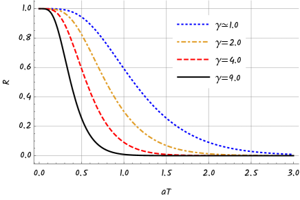
To conduct our analysis, let us rewrite as by convenience, where . In Fig. 1, we have plotted the ratio of the renormalized free energy density, , to the Casimir energy density, , varying with for different values of the parameter .
In each case, the plot shows the ratio going to as approaches zero, as we should expect, and decaying to zero as approaches infinity. In particular, this decay becomes more pronounced as the parameter increases, as illustrated by the curve for . The curves associated with , which decay to zero faster, correspond to the case where is greater than , whereas the curve with illustrates the particular case . In the limiting case when (), the system exhibits a structure known as a quantum spring, as discussed by Feng2010 in the context of the scalar Casimir effect.
In what follows, we will analyze the asymptotic limits of temperature corrections to the massless free energy density above.
IV.2.1 High-temperature limit
Let us analyze the high-temperature limit, , of the final expression (103). In this case, it is more appropriate to perform the summation in first, namely
| (104) |
Inserting this summation into Eq. (103), we are eventually led to the following expression
| (105) |
Note that the first term on the right-hand side in Eq. (IV.2.1), after performing the summation in , gives rise to Casimir energy density associated with massless spinor field (95) but with the opposite sign. Therefore, the effect of this latter term is entirely compensated by the corresponding one in the free energy density (103). Such a natural cancellation between the massless Casimir energy density and its corresponding temperature correction is not unusual. It is an intrinsic characteristic of temperature corrections at the high-temperature limit Plunien1986 .
Now, our task is to evaluate the series (IV.2.1) at a high-temperature limit, (or equivalently ). Through an asymptotic expansion up to terms of order , we arrive at the finite-temperature
| (106) |
which is exponentially suppressed at high and converges to zero as , in accordance with Fig. 1. This behavior is expected for a spinor field since, differently from the scalar field Giulia2021 , it lacks a temperature correction term that is linearly dependent on . We emphasize the need for the free energy density to undergo a finite renormalization by subtracting from it the blackbody radiation contribution, proportional to , to obtain the correct classical limit, a free energy density renormalized to zero at very high temperatures. Ref. Mostepanenko2011 found a similar result for temperature corrections associated with the spinor field in the closed Friedmann cosmological model.
With the renormalized free energy density now available, we can obtain an analytical expression for the renormalized entropy density. Employing the relation (31), we have
| (107) |
The corresponding asymptotic expansion in the high-temperature regime, , decays exponentially with the temperature
| (108) |
Note that the lack of a classical term proportional to in the free energy density results in the Casimir entropy density approaching zero at very high temperatures, which differs from the scalar case where it is dominated by a constant term Giulia2021 .
IV.2.2 Low-temperature limit
Let us now consider the asymptotic expansion of the expression (103) in the low-temperature regime, where , or equivalently . To accomplish this, as previously mentioned, we shall perform the summation in first, providing
| (109) |
Substituting it back in Eq. (103), we get
| (110) |
which at the low-temperature regime up to terms of the order , presents the following free energy density asymptotic behavior
| (111) |
Let us make a few remarks comparing our findings and those reported in Giulia2021 for the low-temperature behavior of the free energy associated with the scalar field under helix topology. Apart from the additional term for temperature correction observed in the scalar case, they differ by constant multiplicative factors that naturally arise because of the spinor degrees of freedom. Note that at small , the above asymptotic expansion is dominated by the first term, the massless Casimir energy density at zero temperature, Eq. (95), as expected Mostepanenko2011 ; Herondy2023 ; Basil1978 .
The entropy density can be obtained by inserting Eq. (IV.2.2) into Eq. (31), providing
| (112) |
Its corresponding asymptotic expansion in the low-temperature limit, where , is found to be
| (113) |
As expected, the above expression tends to zero as the temperature approaches zero. It implies that the entropy density for a massless spinor field satisfying an anti-periodic condition along the compact vector satisfies the third law of thermodynamics (the Nernst heat theorem) Landau1980 .
V Conclusion
In the present work, we have investigated the thermal Casimir effect associated with a massive spinor field defined on a four-dimensional flat space with a circularly compactified dimension. The periodicity represented by is oriented not along a coordinate axis as usual, but along a vector belonging to the -plane, Eq. (59). This geometry introduces a topological constraint inducing a spatial anti-periodic boundary condition on the spinor field, Eq. (61), which modifies the vacuum fluctuations, producing the Casimir effect. Imposing this boundary condition led to the discrete eigenvalues for the momentum along vector , Eq. (64), allowing for determining explicitly the eigenvalues (IV). They are used to construct the generalized zeta function for the spinor field and thus remove the formal divergences involved in the Casimir effect.
These divergencies were introduced by the Dirac operator determinant in the partition function originating from the infinite product over eigenvalues, Eq. (II.1). This divergence was encoded into the generalized zeta function employing the important relation connecting it with the partition function, Eq. (29). It was analyzed from the asymptotic behavior of the spinor heat kernel function, Eq. (44), and removed in the renormalization scheme by subtraction of the divergent contribution associated with non-null heat kernel coefficients. A rather peculiar aspect of the zeta function regularization prescription is related to the existence of ambiguities. Such ambiguities appear whenever the mass-dependent heat kernel coefficient is nonvanishing, Eq. (50), due to natural dependence on parameter , Eq. (III). For the geometry presented here, was the only non-null heat kernel coefficient, Eq. (85), associated with the Euclidean heat kernel contribution, Eqs. (80) and (100). In order to derive physically meaningful expressions, all contributions associated with were dropped to ensure that the renormalization procedure is unique and thus obtain an unambiguous spinor vacuum free energy. Besides that, since is multiplied by mass with a positive exponent, we adopt an additional requirement that vacuum energy should be renormalized to zero for large masses.
We outline all the mathematical machinery required for computing the vacuum-free energy density, starting with the construction of the partition function for the spinor field through Euclidean path integrals. In this Euclidean approach, we find closed and analytical expressions for the vacuum free energy density associated with the spinor field in thermal equilibrium at finite temperature , satisfying anti-periodic conditions in the imaginary time and along vector . This energy density can be expressed as a summation of the zero-temperature Casimir energy density, Eq. (90), and temperature correction terms, Eq. (IV.2), which generalize the results presented in Refs. Bellucci2009 ; Xiang2011 . We also analyzed the high- and low-temperature asymptotic limits, which agree entirely with the curves shown in Fig. 1. The ratio of the renormalized free energy density to the Casimir energy density goes to as approaches zero and decays to zero as approaches infinity. At high temperatures, in particular, we have shown that the coefficient gives rise to the Stefan-Boltzmann law, proportional to . Although not divergent, this quantum term was subtracted in the renormalization procedure to obtain a correct classical contribution in this limit. Also, the free energy density does not possess a classical limit at high temperatures. Except for this classical limit, all our results for spinor fields differ from the ones for scalar fields by constant multiplicative factors that naturally arise because of the spinor degrees of freedom. Finally, our analysis confirms that the entropy density agrees with the Nernst heat theorem.
VI Acknowledgments
J. V. would like to thank Fundação de Amparo a Ciência e Tecnologia do Estado de Pernambuco (FACEPE), for their partial financial support. A. M. acknowledges financial support from the Brazilian agencies Conselho Nacional de Desenvolvimento Científico e Tecnológico (CNPq), grant no. 309368/2020-0 and Coordenação de Aperfeiçoamento de Pessoal de Nível Superior (CAPES). H. M. is partially supported by CNPq under grant no. 308049/2023-3. L. F. acknowledges support from CAPES, financial code 001.
References
- (1) H. B. G. Casimir, On the Attraction Between Two Perfectly Conducting Plates, Indag. Math. 10, 261 (1948).
- (2) M. J. Sparnaay, Measurements of attractive forces between flat plates, Physica 24, 751 (1958).
- (3) G. Bressi, G. Carugno, R. Onofrio, and G. Ruoso, Measurement of the Casimir force between parallel metallic surfaces, Phys. Rev. Lett., 88, 041804 (2002).
- (4) S. K. Lamoreaux, Erratum: Demonstration of the casimir force in the 0.6 to 6 µm range, Phys. Rev. Lett. 81, 5475 (1998).
- (5) S. K. Lamoreaux, Demonstration of the Casimir force in the 0.6 to 6 micrometers range, Phys. Rev. Lett. 78, 5 (1997). Erratum: Phys.Rev.Lett. 81, 5475 (1998).
- (6) U. Mohideen and A. Roy, Precision measurement of the Casimir force from 0.1 to 0.9 micrometers, Phys. Rev. Lett. 81 4549 (1998).
- (7) M. Bordag, U. Mohideen, and V. M. Mostepanenko, New developments in the Casimir effect, Phys. Rept. 353, 1 (2001).
- (8) V. M. Mostepanenko and N. N. Trunov, The Casimir effect and its applications (Clarendon Press, Oxford, New York, 1997).
- (9) L. H. Ford, Quantum vacuum energy in general relativity, Phys. Rev. D 11, 3370 (1975).
- (10) J. S. Dowker and R. Critchley, Covariant Casimir calculations, J. Phys. A 9, 535 (1976).
- (11) J. S. Dowker, Thermal properties of Green’s functions in Rindler, de Sitter, and Schwarzschild spaces, Phys. Rev. D 18, 1856 (1978).
- (12) T. Appelquist and A. Chodos, Quantum Effects in Kaluza-Klein Theories, Phys. Rev. Lett. 50, 141 (1983).
- (13) Y. Hosotani, Dynamical gauge symmetry breaking as the Casimir effect, Phys. Lett. B 129, 193 (1983).
- (14) I. Brevik, K.A. Milton, S.D. Odintsov, Entropy Bounds in Geometries, Ann. Phys. 302, 120 (2002).
- (15) A. Zhang, Thermal Casimir Effect in Kerr Space-time, Nuclear Physcis B 898, 2020, (2015).
- (16) C. Henke, Quantum vacuum energy in general relativity, Eur. Phys. J. C 78, 126 (2018).
- (17) K. Bradonjic, J. Swain, A. Widom, and Y. Srivastava, The casimir effect in biology: The role of molecular quantum electrodynamics in linear aggregations of red blood cells, Journal of Physics: Conference Series 161, 012035 (2009).
- (18) Peng Liu and Ji-Huan He, Geometric potential: An explanation of nanofibers wettability, Thermal Science 22, 33 (2018).
- (19) P. Pawlowski and P. Zielenkiewicz, The quantum casimir effect may be a universal force organizing the bilayer structure of the cell membrane, The Journal of membrane biology 246, 383 (2013).
- (20) A. Gambassi, The Casimir effect: From quantum to critical fluctuations, J. Phys. Conf. Ser. 161, 012037 (2009).
- (21) B. B. Machta, S. L. Veatch, and J. P. Sethna, Critical casimir forces in cellular membranes, Phys. Rev. Lett. 109, 138101 (2012).
- (22) G. L. Klimchitskaya, U. Mohideen and V. M. Mostepanenko, The Casimir force between real materials: Experiment and theory, Rev. Mod. Phys. 81, 1827 (2009).
- (23) K. Milton and I. Brevik, Casimir Physics Applications, Symmetry 11, 201 (2019).
- (24) K. A. Milton, The Casimir Effect: Physical Manifestation of Zero-Point Energy (World Scientific, Singapore, 2001).
- (25) M. Bordag, G. L. Klimchitskaya, U. Mohideen, and V. M. Mostepanenko, Advances in the Casimir effect (Oxford University, Press, Oxford, 2009), Vol. 145.
- (26) A. Stokes and R. Bennett, The Casimir effect for fields with arbitrary spin, Annals Phys. 360, 246 (2015).
- (27) C. Farina, The Casimir Effect: Some Aspects. Brazilian Journal of Physics 36, 1137 (2006).
- (28) C. R. Muniz, M. O. Tahim, M. S. Cunha and H. S. Vieira, On the global Casimir effect in the Schwarzschild spacetime, JCAP 1801, 006 (2018).
- (29) M. S. Cunha, C. R. Muniz, H. R. Christiansen, V. B. Bezerra, Relativistic Landau levels in the rotating cosmic string spacetime, Eur. Phys. J. C 76, 512 (2016).
- (30) S. Mobassem, Casimir effect for massive scalar field, Mod. Phys. Lett. A 29, 1450160 (2014).
- (31) S. H. Pereira, J. M. Hoff da Silva and R. dos Santos, Casimir effect for Elko fields, Mod. Phys. Lett. A 32, 1730016 (2017).
- (32) A. A. Bytsenko, M. E. X. Guimarães and V. S. Mendes, Casimir Effect for Gauge Fields in Spaces with Negative Constant Curvature, Eur. Phys. J. C 39, 249 (2005).
- (33) M. N. Chernodub, V. A. Goy, A. V. Molochkov and Ha Huu Nguyen, Casimir effect in Yang-Mills theory, Phys. Rev. Lett. 121, 191601 (2018)
- (34) A. Edery, Casimir piston for massless scalar fields in three dimensions, Phys. Rev. D 75 (2007) 105012, [hep-th/0610173].
- (35) E. Ponton and E. Poppitz, Casimir Energy and Radius Stabilization in Five and Six Dimensional Orbifolds, JHEP 0106, 019 (2001).
- (36) E. Cartan, The Theory of Spinors, Dover (1966).
- (37) I. Benn and R. Tucker, An Introduction to spinors and geometry with applications in physics, Adam Hilger, Bristol (1987).
- (38) J. Venâncio, The spinorial formalism. Lambert Academic Publishing, Germany (2019).
- (39) V. K. Oikonomou and N. D. Tracas, Slab Bag Fermionic Casimir effect, Chiral Boundaries and Vector Boson-Majorana Fermion Pistons, Int. J. Mod. Phys. A 25, 5935 (2010).
- (40) H. Cheng, Casimir effect for parallel plates involving massless Majorana fermions at finite temperature, Phys. Rev. D 82, 045005 (2010).
- (41) R. M. Cavalcanti, Casimir force on a piston, Phys. Rev. D 69, 065015 (2004).
- (42) E. Elizalde, Zeta function methods and quantum fluctuations, J. Phys. A 41, 304040 (2008).
- (43) E. Elizalde, Ten Physical Applications of Spectral Zeta Functions (Springer, New York, 1995).
- (44) S. W. Hawking, Zeta function regularization of path integrals in curved spacetime, Commun. math. Phys. 55, 133 (1977).
- (45) E. Elizalde, Zeta function regularization in Casimir effect calculations and J.S. Dowker’s contribution, Int. J. Mod. Phys. A 27, 1260005 (2012).
- (46) E. Elizalde, S. D. Odintsov, A. Romeo, A. A. Bytsenko, and S. Zerbini, Zeta regularization techniques with applications, World Scientific (1994).
- (47) M. Basil Altaie and J. S. Dowker, Spinor fields in an Einstein universe: Finite-temperature effects, Phys. Rev. D 18, 3557 (1978).
- (48) G. Plunien, B. Muller and W. Greiner, The Casimir effect, Phys. Rept. 134, 87 (1986).
- (49) I. K. Kulikov, P. I. Pronin. Finite temperature contributions to the renormalized energy-momentum tensor for an arbitrary curved space-time. Czech J Phys 38, 121 (1988).
- (50) R. V. Maluf, D. M. Dantas and C. A. S. Almeida, The Casimir effect for the scalar and Elko fields in a Lifshitz-like field theory, Eur. Phys. J. C 80, 442 (2020).
- (51) M. Kac, Can one hear the shape of a drum? Amer. Math. Monthly 73, 1 (1966).
- (52) M. Bordag, Ground state energy for massive fields and renormalization, Commun. Mod. Phys., Part D 1, 347 (2000).
- (53) D. V. Vassilevich, Heat kernel expansion: user’s manual, Phys. Rept. 388, 279 (2003).
- (54) K. Kirstein, Basic zeta functions and some applications in physics, 2010. arXiv:1005.2389
- (55) T. Branson and P. Gilkey, Residues of the eta function for an operator of Dirac type, J. Funct. Anal. 108, 47 (1992).
- (56) T. Branson and P. Gilkey, Residues of the eta function for an operator of Dirac type with local boundary condtitons, Differential Geom. Appl. 2, 249 (1992).
- (57) A. Chodos, R. L. Jaffe, K. Johnson, C. B. Thorn, and V. F. Weisskopf, New extended model of hadrons, Phys. Rev. D 9, 3471 (1974).
- (58) K. Johnson, The M.I.T. bag model, Acta Phys. Polon. B 6, 865 (1975).
- (59) N. Arrizabalaga, L. Le Treust and N. Raymond, On the MIT bag model in the non-relativistic limit, Commun. Math. Phys. 354, 641 (2017).
- (60) S. G. Mamayev and N. N. Trunov, Vacuum expectation values of the energy-momentum tensor of quantized fields on manifolds with different topologies and geometries. III, Sov. Phys. J. 23, 551, (1980).
- (61) A. Erdas, Finite temperature Casimir effect for massless Majorana fermions in a magnetic field, Phys. Rev. D 83, 025005 (2011).
- (62) E. Elizalde et al., The Casimir energy of a massive fermionic field confined in a -dimensional slab-bag, International Journal of Modern Physics A 18, 1761 (2012).
- (63) E. Elizalde, M. Bordag and K. Kirsten, Casimir energy for a massive fermionic quantum field with a spherical boundary, J. Phys. A: Math. Gen. 31, 1743 ( 1998).
- (64) C. M Bender and P. Hays, Zero-point energy of fields in a finite volume, Phys. Rev. D 14, 2622 (1976).
- (65) G. Fucci and C. Romaniega, Casimir energy for spinor fields with -shell potentials, J. Phys. A: Math. Theor. 56, 265201 (2023).
- (66) S. H. Pereira and R. S. Costa, Partition function for a mass dimension one fermionic field and the dark matter halo of galaxies, Mod. Phys. Lett. A 34, 1950126 (2019).
- (67) Xiang-hua Zhai, Xin-zhou Li, Chao-Jun Feng, Casimir effect with a helix torus boundary condition, Mod. Phys. Lett. A 26, 1953 (2011).
- (68) K. E. L. de Farias and H. F. Santana Mota, Quantum vacuum fluctuation effects in a quasi-periodically identified conical spacetime, Phys. Lett. B 807 (2020) 135612, [arXiv:2005.03815].
- (69) Chao-Jun Feng and Xin-zhou Li, Quantum Spring from the Casimir Effect, Phys. Lett. B 691 (2010) 167–172, [arXiv:1007.2026].
- (70) Xiang-hua Zhai, Xin-zhou Li, Chao-Jun Feng, The Casimir force of Quantum Spring in the (D+1)-dimensional spacetime, Mod. Phys. Lett. A 26 (2011) 669–679, [arXiv:1008.3020].
- (71) Chao-Jun Feng and Xin-zhou Li, Quantum Spring, Int. J. Mod. Phys. Conf. Ser. 7 (2012) 165–173, [arXiv:1205.4475].
- (72) H. F. Mota and V. B. Bezerra, Topological thermal Casimir effect for spinor and electromagnetic fields, Phys. Rev. D 92, 124039 (2015).
- (73) K. E. L. de Farias, A. Mohammadi, and H. F. Santana Mota, Thermal Casimir effect in a classical liquid in a quasi-periodically identified conical spacetime, Phys. Rev. D 105, 085024 (2022).
- (74) H. Mota, Vacuum energy, temperature corrections and heat kernel coefficients in -dimensional spacetimes with nontrivial topology, 2023. arXiv:2312.01909
- (75) V. B. Bezerra, V. M. Mostepanenko, H. F. Mota, and C. Romero, Thermal Casimir effect for neutrino and electromagnetic fields in the closed Friedmann cosmological model, Phys. Rev. D 84, 104025 (2011).
- (76) N. D. Birrell and L. H. Ford, Renormalization of Self-Interacting Scalar Field Theories in a Nonsimply Connected Spacetime. Physical Review D 22, 330 (1980).
- (77) Xiang-hua Zhai, Xin-zhou Li and Chao-Jun Feng, Fermionic Casimir effect with helix boundary condition, Eur. Phys. J. C 71, 1654 (2011).
- (78) S. Bellucci, A.A. Saharian, Fermionic Casimir effect for parallel plates in the presence of compact dimensions with applications to nanotubes, Phys. Rev. D 80, 105003 (2009).
- (79) G. Aleixo, H. F. Santana Mota, Thermal Casimir effect for the scalar field in flat spacetime under a helix boundary condition, Phys. Rev. D 104, 045012 (2021).
- (80) Chao-Jun Feng, Xin-Zhou Li, Xiang-Hua Zhai, Casimir Effect under Quasi-Periodic Boundary Condition Inspired by Nanotubes, Mod. Phys. Lett A 29, 1450004 (2014
- (81) B. Liu, C. L. Yuan, H. L. Hu, et al. Dynamically actuated soft heliconical architecture via frequency of electric fields. Nat Commun 13, 2712 (2022).
- (82) I. Greenfeld, I. Kellersztein and H. D. Wagner, Nested helicoids in biological microstructures. Nat Commun 11, 224 (2020).
- (83) E. Elizalde and A. Romeo, Heat-kernel approach to zeta function regularization of the Casimir effect for domains with curved boundaries, Int. J. Mod. Phys. A 5, 1653, (1990).
- (84) R.T. Seeley, Complex powers of an elliptic operator, Amer. Math. Soc. Proc. Symp. Pure Math. 10, 288 (1967).
- (85) D. V. Vassilevich, Operators, Geometry and Quanta, Springer (2011).
- (86) P. Gilkey, Invariance Theory, the Heat Equation, and the Atiya-Singer Index Theorem. CRC Press, Boca Raton, FL, 1995.
- (87) I. K. Kulikov and P. I. Pronin, Topology and chiral symmetry breaking in four-fermion interaction, Acta Phys. Polon. B 20, 713 (1989).
- (88) N. Ahmadi and M. Nouri-Zonoz, Massive spinor fields in flat spacetimes with non-trivial topology, Phys. Rev. D 71, 104012 (2005).
- (89) J. Venâncio and C. Batista, Separability of the Dirac equation on backgrounds that are the direct product of bidimensional spaces, Physical Review D 95, 084022 (2017).
- (90) S. S. Gousheh, A. Mohammadi, and L. Shahkarami, Casimir energy for a coupled fermion-kink system and its stability, Phys. Rev. D 87, 045017 (2013).
- (91) A. Mohammadi, E. R. Bezerra de Mello and A. A. Saharian, Induced fermionic currents in de Sitter spacetime in the presence of a compactified cosmic string, Class. Quantum Grav. 32, 135002 (2015).
- (92) E. A. F. Bragança, E. R. Bezerra de Mello, and A. Mohammadi, Induced fermionic vacuum polarization in a de Sitter spacetime with a compactified cosmic string, Phys. Rev. D 101, 045019 (2020).
- (93) A. Bytsenko, L. Vanzo, S. Zerbini, Zeta-function regularization approach to finite temperature effects in Kaluza-Klein space-times, Mod. Phys. Lett. A 7, 2669 (1992).
- (94) S. Zerbini, Spinor fields on topologically nontrivial spacetime, Letters in Mathematical Physics 27, 19 (1993).
- (95) L. D. Landau and E. M. Lifshitz, Statistical Physics, Part I. Pergamon Press, Oxford, 1980.
- (96) C.J. Feng, X.Z. Li, Quantum spring from the Casimir effect, Phys. Lett. B 691, 167 (2010).
- (97) M. Abramowitz and I. A. Stegun, Handbook of Mathematical Functions with Formulas, Graphs, and Mathematical Tables (Dover, New York, 1972).