Excited-State Dynamics and Optically Detected Magnetic Resonance of Solid-State Spin Defects from First Principles

Abstract

Optically detected magnetic resonance (ODMR) is an efficient and reliable method that enables initialization and readout of spin states through spin-photon interface. In general, high quantum efficiency and large spin-dependent photoluminescence (PL) contrast are desirable for reliable quantum information readout. However, reliable prediction of the ODMR contrast from first-principles requires accurate description of complex spin polarization mechanisms of spin defects. These mechanisms often include multiple radiative and nonradiative processes in particular intersystem crossing (ISC) among multiple excited electronic states. In this work we present our implementation of the first-principles ODMR contrast, by solving kinetic master equation with calculated rates from ab initio electronic structure methods then benchmark the implementation on the case of the negatively-charged nitrogen vacancy (NV) center in diamond. We show the importance of correct description of multi-reference electronic states for accurate prediction of excitation energy, spin-orbit coupling, and the rate of ISC. Moreover, we underscore the importance of pseudo Jahn-Teller effect for the spin-orbit coupling, and the dynamical Jahn-Teller effect for electron-phonon coupling, key factors determining ISC rates and ODMR contrast. We show good agreement between our first-principles calculations and the experimental ODMR contrast under magnetic field. We then demonstrate reliable predictions of magnetic field direction, pump power, and microwave frequency dependency, as important parameters for ODMR experiments. Our work clarifies the important excited-state relaxation mechanisms determining ODMR contrast and provides a predictive computational platform for spin polarization and optical readout of solid-state quantum defects from first principles.

I Introduction

Point defects in solids as spin qubits offer multiple revenues to quantum technologies, in particular quantum sensing and quantum networking [1]. The promising candidates exhibit long quantum coherence times [2, 3, 4], essential for performing multi-step quantum operations with high fidelity. They are relatively scalable and easy to integrate into existing technologies due to their solid-state nature [5]. Furthermore, they can be optically initialized and reliably read out in a wide temperature range [6, 7, 8], through the spin-photon entanglement [9]. While discovering and exploring new spin defects beyond the extensively-studied negatively-charged nitrogen-vacancy (NV) center in diamond [10] has been a key interest in recent years, reliable theoretical predictions of optical readout properties remain challenging, which hinder rapid progress.

The first outstanding issue is the missing link between experimental observable and first-principles simulations for the spin polarization processes. The experimental tool to study spin polarization is through optically detected magnetic resonance (ODMR) [11, 12, 13, 14], by recording photoluminescence contrast with and without microwave radiation as a function of magnetic field. This requires to solve the kinetic equations for excited-state occupations of different spin sublevels. The excited-state occupation is determined by kinetic processes in the polarization cycle, including radiative and nonradiative recombination between different spin states. Previously, only model simulations with experimental rates and energy levels to describe ODMR have been reported [11, 12, 13, 14]. A first-principles formalism and computational tool is yet to be developed in order to interpret experiments or predict ODMR of new spin defect systems.

To perform first-principles ODMR, predictions of optical excitation energies, zero-field splitting, radiative and nonradiative recombination rates are required. Various first-principles electronic structure methods have been proposed to calculate excitation energies of spin defects. The key consideration is to accurately capture the electron correlation of defect states. For instance, mean-field theory such as constrained DFT (CDFT) [15] could provide reasonable structural and ground state information, but GW and solving the Bethe-Salpeter Equation (GW-BSE) can provide more accurate quasiparticle energies and optical properties including electron-hole interactions [16, 17]. On the other hand, if the defect states have strong multi-reference nature, such as open-shell singlet excited state of the NV center, theories like quantum-defect-embedding theory (QDET) for solids [18, 19] or multi-reference wavefunction methods [20] may be more appropriate.

The first-principles theory for excited-state kinetic properties of spin defects has recent advancement as well. For example, the radiative recombination rates have been calculated at finite temperature with inputs from many-body perturbation theory for better description of excitons [18, 21]. The nonradiative recombination transitions, in particular intersystem crossing (ISC) that requires spin-flip transition and phonon-assisted internal conversion (IC), can be obtained from phonon perturbation to electronic state [22, 16, 23, 15]. However, these calculations have not considered the multi-reference nature of the electronic states and complex Jahn-Teller (JT) effects coupled in the kinetic processes.

In this work, we have developed the first-principles ODMR theory and computational tool to directly predict ODMR contrast without prior input parameters as shown in Fig. 1(a). We note that such tool is fully general to all solid-state defect systems, although we first use the NV center as a prototypical example. By combining advanced electronic structure methods and group theory analysis, we discuss the significance of Coulomb repulsion, pseudo JT and dynamical JT effects to the SOC and ISC. The consideration of these effects facilitates the interpretation of the experimentally observed ISC rates that essentially contribute to spin polarization. We predict the ODMR contrast as a function of an external magnetic field fully from first-principles. We demonstrate that these simulations are invaluable for predicting spin-polarization mechanism and provide control strategy on high fidelity optical initialization and readout.

II Computational Methods

We carried out first-principles calculations of structural and ground-state properties using the open-source plane-wave code Quantum Espresso [24]. The NV center defect is introduced into a diamond crystal with $3\times 3\times 3$ supercell size, containing 216 atoms. Only Gamma point is sampled in the Brilloin zone of the defect supercells. We use the optimized norm-conserving Vanderbilt (ONCV) pseudopotentials [25] with the wavefunction energy cutoff of 70Ry. The lattice constant is optimized by using the exchange-correlation functional with the Perdew-Burke-Ernzerhof (PBE) generalized gradient approximation [26]. For comparison, we also used the range-separated hybrid function proposed by Heyd, Scuseria, and Ernzerhof (HSE) [27, 28]. The HSE functional has been shown to better describe the electronic structure of the NV center in diamond compared to the PBE functional [29, 30, 31]. We calculate the excitation energies using three different methods, constrained DFT (CDFT), single-shot GW plus the Bethe-Salpeter Equation ($\text{G}_{0}\text{W}_{0}\text{-}\text{BSE}$), and complete active space self-consistent field (CASSCF) method in quantum chemistry [32].

The many-body perturbation theory calculations are performed by using the Yambo-code [33], with PBE eigenvalues and wavefunctions as the starting point for quasiparticle energies at GW approximation. For the dynamical screening, we take the Godby-Needs plasmon-pole approximation (PPA) [34, 35]. We then solve the Bethe-Salpeter Equation (BSE) for two-particle excitation, specifically for optical excitation energies and transition dipole moments including explicit electron-hole interactions. A $2\times 2\times 2$ supercell is used for the $\text{G}_{0}\text{W}_{0}\text{-}\text{BSE}$ calculations, and the results are comparable to the previous reported values [18].

Due to the multi-reference character of the ${}^{3}E$, ${}^{1}E$, and ${{}^{1}A_{1}}$ excited states of the NV center, a single Slater determinant description in DFT is incomplete. To overcome this problem, we use the CASSCF method [32] to construct the state wavefunctions as linear combinations of multiple Slater determinants. Each determinant describes a particular occupation of single-electron orbitals. In the CASSCF method, the orbital space is partitioned into subspaces of the inactive, active, and virtual orbitals. The occupation of the active orbitals is allowed to change to generate all possible spin- and symmetry-allowed determinants for a particular electronic state. A choice of a partition of the orbital space, that is the choice of a number of active orbitals and active electrons, determines the CASSCF active space. We use the state-average (SA) version of the CASSCF method as implemented in ORCA [36, 37] to obtain state wavefunctions for calculations of SOC matrix elements. Specifically, we perform SA(10)-CASSCF(4,6) calculations, where SA(10) refers to state-averaging over ten states, which include five singlet and five triplet states, and CASSCF(4,6) refers to four electrons and six orbitals included in the active space. The second order Douglas-Kroll-Hess (DKH2) Hamiltonian [38] and the cc-pVDZ-DK basis set [39, 40] were used to account for the scalar relativistic effects. The spin-orbit mean-field operator was used [41].

III Results and Discussion

III.1 ODMR Theory, Implementation, and Benchmark

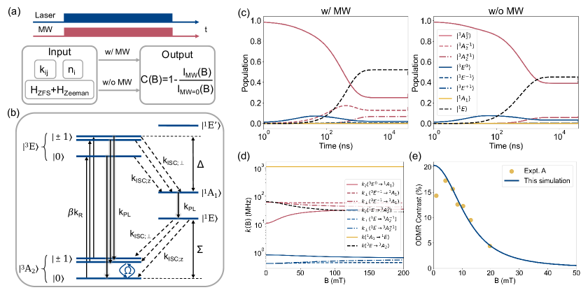
Figure 1: Numerical implementation of ODMR contrast and its benchmark with the NV center in diamond. (a) The continuous-wave (cw) ODMR and its simulation workflow with first-principles inputs. (b) Schematic diagram depicting the energy levels and excited-state kinetic processes of the NV center in diamond. $\ket{0}$, $\ket{-1}$ and $\ket{+1}$ denote the spin sublevels in the triplet states. The spin sublevels $\ket{+1}$ and $\ket{-1}$ are degenerate under zero magnetic field. (c) The time-evolved populations of the states reach a steady-state plateau with sufficiently long time, in the presence (w/MW, left panel) or absence (w/o MW, right panel) of microwave field. (d) Transition rates ($k$) for different processes vary differently with magnetic field B. (e) Simulated ODMR contrast as a function of magnetic field (solid line) and compared with the experiment (dots) [11]. The experimental data is extracted from a figure by using WebPlotDigitizer tool [42].

The basic mechanism of ODMR is related to the excited-state populations of spin sublevels. Therefore, we begin with the Hamiltonian that describes the spin sublevels of triplet states as in Fig. 1(b),

$$H_{\text{s}} =D(S_{z}^{2}-\frac{\mathbf{S}^{2}}{3})+E(S_{x}^{2}-S_{y}^{2})+g_{e}\mu_{B}\mathbf{B}\cdot\mathbf{S}$$ (1)

where $S_{i}$ is the spin-1 operator along $i$ axis, $D$ in the first term is the axial zero-field splitting (ZFS) parameter, $E$ in the second term is the rhombic ZFS parameter, $g_{e}$ is the electron g-factor or gyromagnetic ratio whose value is ${\sim}2$ in the NV center, $\mu_{B}$ is Bohr magneton, and $\mathbf{B}$ is the external magnetic field. The ZFS lifts the spin degeneracy. The third term describes the Zeeman effect occuring under magnetic field ($\mathbf{B}$) and further leading to the mixing of the original spin sublevels. Let $\alpha_{ij}$ be the mixing coefficient of original spin sublevels $\ket{i}$ and $\ket{j}$, then we can write the transition rates under magnetic field $k_{ij}(\mathbf{B})$ to be a function of mixing coefficients and the rates at zero magnetic field ($k^{0}_{pq}$),

$$k_{ij}(\mathbf{B}) =\sum_{p,q}|\alpha_{ip}(\mathbf{B})|^{2}|\alpha_{jq}(\mathbf{B})|^{2}k^{0}_{pq}.$$ (2)

The spin mixing will be shown below to be the source of the magnetic field-dependent ODMR.

We then numerically implement the ODMR contrast based on the kinetic master equation [11, 43], which integrates all transition rates and allows to simulate the dynamics of states populations, photoluminescence (PL) intensity, as well as continuous wave (cw) or time-resolved ODMR. The model starts with the conventional definition of ODMR contrast,

$$\begin{split}C(\mathbf{B})=1-\frac{\bar{I}(t,\mathbf{B},k_{\mathrm{MW}})}{\bar{I}(t,\mathbf{B},k_{\mathrm{MW}}=0)}\end{split}$$ (3)

$$\begin{split}\bar{I}(t,\mathbf{B})=\eta\sum_{i\in\mathrm{ES}}\sum_{j\in\mathrm{GS}}k_{ij}(\mathbf{B})\bar{n}_{i}(t,\mathbf{B})\end{split}$$ (4)

where $\bar{I}(t,\mathbf{B},k_{\mathrm{MW}})$ is the magnetic-field dependent PL intensity at the steady state in the presence of microwave resonance (MW), which is different from the case in the absence of microwave resonance ($k_{\mathrm{MW}}=0$). Here, $k_{\mathrm{MW}}$ is the Rabi frequency of a microwave field that is applied for rotating the populations of spin sublevels, and is a parameter in the model as it scales with the amplitude of the microwave field [44]. $\eta$ is the collection coefficient parameter for PL intensity which depends on experimental setup but does not affect ODMR. The optical saturation parameter $\beta$ seen in Fig. 1(b) and SM Sec. I plays a role in the optical excitation. Both $k_{\mathrm{MW}}$ and $\beta$ are determined according to the experimental range [11]. The PL intensity evolves with time depending on $n_{i}(t,\mathbf{B})$, the population of spin level $\ket{i}$ at time $t$, and can be solved numerically using the Euler method.

To validate the ODMR contrast implementation for triplet systems, we firstly simulate the ODMR of the prototypical system NV center, as shown in Fig. 1(b), using the experimental values of ZFS and rates [11, 45, 43]. The purpose of this benchmark is to confirm the numerical implementation of ODMR contrast from Eq. (1) to Eq. (4), independent of the accuracy of electronic structure and kinetic rates, which will be discussed in detail in the next sections. Values for the ODMR simulation parameters are tabulated in SM Table S1, and the microwave resonance is applied to drive the rotation between $\ket{\prescript{3}{}{A}_{2}^{0}}$ and $\ket{\prescript{3}{}{A}_{2}^{-1}}$. Since the simulated cw-ODMR is observed at steady state, arbitrary initial populations of the spin sublevels can be used. The system reaches the steady state after ${\sim}10^{4}$ ns, as shown in Fig. 1(c). From the steady-state populations, we can find that $\ket{\prescript{3}{}{A}_{2}^{-1}}$ has larger population due to the Rabi oscillation in the presence of the microwave field compared to the absence of the microwave field. Because the optical excitation is mostly spin-conserving [46], the population of $\ket{\prescript{3}{}{E}^{-1}}$ is subsequently larger. Because the nonaxial ISC $\prescript{3}{}{E}\rightarrow\prescript{1}{}{A}_{1}$ is symmetrically allowed and fast, as can be seen in Fig. 1(d), it competes with the radtiative recombination $\prescript{3}{}{E}\rightarrow\prescript{3}{}{A}_{2}$, leading to overall smaller excited-state population. Therefore, the PL intensity in the presence of the microwave field becomes smaller, and the ODMR contrast is positive as shown in Fig. 1(e). The decrease of ODMR contrast with the magnetic field is a consequence of the smaller difference between axial ISC rates and nonaxial ISC rates, compared Fig. 1(d) to Fig. 1(e). The fundamental reason is the mixing of spin sublevels, which will be discussed in details in Sec. III.6. To understand the magnetic field effect, first, when the magnetic field is misaligned with the NV axis, there is mixing between spin sublevels $m_{s}=0$ and $m_{s}=\pm 1$. Second, the spin mixing will further mix ISC rates between different transitions as Eq. (2).For the NV center, the spin polarization is mainly a result of $k_{\perp}(\prescript{3}{}{E}\rightarrow\prescript{1}{}{A}_{1})\gg k_{z}(\prescript{3}{}{E}\rightarrow\prescript{1}{}{A}_{1})$. When $k_{\perp}(\prescript{3}{}{E}\rightarrow\prescript{1}{}{A}_{1})$ is similar to $k_{z}(\prescript{3}{}{E}\rightarrow\prescript{1}{}{A}_{1})$ due to spin mixing, spin polarization is weaker, ODMR contrast is smaller. The excellent agreement of our simulation with experiment in Fig. 1(e) validates the numerical implementation of ODMR.

Besides triplet spin defects, singlet defects that have a triplet metastable state can also show ODMR signal, like ST1 defect in diamond [47, 48]. In SM Sec. I, we additionally include the detailed benchmark of the ODMR model for singlet spin defect. The benchmark for both triplet and singlet spin defects demonstrates the generality of the ODMR model.

Next, we will discuss in detail the first-principles calculations of electronic structure and excited-state kinetic rates at solid-state spin defects, specifically the NV center here.

III.2 Electronic Structure, Excitation Energies and Radiative Recombination of NV Center 

Table 1: The excitation energies of the NV center from various theories along with experiments. The energy of $\prescript{3}{}{A}_{2}$ is aligned to 0 eV, and the energies of the other states are entered with respect to $\prescript{3}{}{A}_{2}$. $\Sigma$ is the excitation energy of $\prescript{1}{}{E}$ with respect to $\prescript{3}{}{A}_{2}$, and $\Delta$ is the energy difference between $\prescript{3}{}{E}$ and $\prescript{1}{}{A}_{1}$, as illustrated in Fig. 1(b).

Method	$\prescript{1}{}{E}$ or $\Sigma$ (eV)	$\prescript{1}{}{A}_{1}$ (eV)	$\prescript{3}{}{E}$ (eV)	$\Delta$ (eV)
Expt. (ZPL)	0.325-0.411	1.515-1.601 [49, 50, 45]	1.945 [51, 52, 53]	0.344-0.430 [52, 53]
Expt. (abs)	–	1.76 [45]	2.180 [51]	–
CDFT (ZPL, HSE, this work)	0.37	–	1.95	–
GW-BSE@PBE (this work, absorption)	-	-	2.25	-
CASSCF (this work)	0.59	1.68	2.05	0.36

The NV center comprises a substitutional nitrogen atom and a vacancy with one extra electron in the faced-center cubic diamond, with its local structure described by the $C_{3v}$ symmetry point group. The three-fold symmetry axis is the nitrogen-vacancy axis along the [111] direction. The ground and low-lying excited electronic states of the NV center can be determined from two one-electron orbitals, $a_{1}$ and $e$ ($e_{x}$, $e_{y}$), which transform as the $A_{1}$ and $E$ irreducible representations of the $C_{3v}$ point group, respectively. These one-electron orbitals are formed by the carbon and nitrogen dangling bonds near the vacancy defect. The $a_{1}^{2}e^{2}$ configuration gives rise to the ${{}^{3}A_{2}}$, ${{}^{1}E}$ and ${{}^{1}A_{1}}$ states, and $a_{1}e^{3}$ to the ${{}^{3}E}$ and ${{}^{1}E^{\prime}}$ states. The states above are listed in the ascending energy order determined experimentally for all the states except ${{}^{1}E^{\prime}}$ whose relative energy is determined from the group theory [50, 45, 52, 15]. The total spin-orbit irreducible representations of these states are given in SM Table S3. The derivation of the representations can be found in literature [54, 55, 56].

Excitation energies play an important role in energy conservation in radiative (electron-photon interaction) and nonradiative (electron-phonon interaction) recombination rates. As we discussed earlier, the excited states of defects can have multi-reference character which is difficult to describe by conventional DFT. Therefore we show the calculated excitation energies from several different electronic structure methods, CDFT, $\text{G}_{0}\text{W}_{0}\text{-}\text{BSE}$@PBE and CASSCF, as listed in Table 1. With all three methods, we obtain excitation energies of triplet excited-state $\prescript{3}{}{E}$ in good agreement with experiments. However, only in the CASSCF calculation we can obtain the excitation energy of the $\prescript{1}{}{A}_{1}$ state, which has a multi-reference character. We also include the higher-lying ${{}^{1}E^{\prime}}$ state in the state-averaging to account for the Coulomb repulsion that couples the ${{}^{1}E}$ and ${{}^{1}E^{\prime}}$ states. More discussion about the excitation energies can be found in SM Sec. II A.

With the excitation energies, we employ the Fermi’s golden rule to calculate radiative recombination rate. The details of calculation methods can be found in our past work [21, 22, 16] and results can be found in SM Sec. III B. For the convenience of comparing our calculated results with previous experiment and calculations, here we adopt lifetime ($\tau$), which is the inverse of rate ($\tau=1/k$). Using the optical dipole moments and excitation energy from $\text{G}_{0}\text{W}_{0}\text{-}\text{BSE}$@PBE calculations which includes excitonic effect accurately, we obtain $\tau_{\text{R}}=$16.8 ns for the $\prescript{3}{}{E}\rightarrow\prescript{3}{}{A}_{2}$ transition and 3061 ns for the $\prescript{1}{}{A}_{1}\rightarrow\prescript{1}{}{E}$ transition. Our calculated radiative lifetimes are consistent with experiment 12 ns for $\prescript{3}{}{E}\rightarrow\prescript{3}{}{A}_{2}$ [52], and previous calculations, ${\sim}10$ ns for $\prescript{3}{}{E}\rightarrow\prescript{3}{}{A}_{2}$ and 1878 ns for $\prescript{1}{}{A}_{1}\rightarrow\prescript{1}{}{E}$ [18, 57].

III.3 Spin-Orbit Coupling and Pseudo Jahn-Teller Effect 

Spin-orbit coupling Hamiltonian can be separated into the axial/nonaxial SOC components ($\lambda_{z/\perp}$) with the angular momentum ladder operators ($L_{\pm}$ and $S_{\pm}$) and $z$ components ($L_{z}$ and $S_{z}$),

$$H_{\text{soc}} =\frac{\lambda_{\perp}}{2}(L_{+}S_{-}+L_{-}S_{+})+\lambda_{z}L_{z}S_{z}.$$ (5)

Table 2: Summary of SOC matrix elements predicted by group theory, calculated at the theory levels of CASSCF and TDDFT, and from experiment. The unit is GHz. CASSCF ($C_{3v}$) SOCs are consistent with prediction. TDDFT ($C_{3v}$) SOCs are inconsistent with group theory. “CR” stands for Coulomb repulsion that mixes $\prescript{1}{}{E}$ and ${{}^{1}E^{\prime}}$. Pseudo JT effect mixes $\prescript{1}{}{A}_{1}$ and $\prescript{1}{}{E}$ through electron-phonon coupling, leading to nonzero SOCs. “–” denotes value that does not exist or that is not found.

	$\lambda_{z}(\prescript{3}{}{E},\prescript{3}{}{E})$	$\lambda_{\perp}(\prescript{1}{}{A}_{1},\prescript{3}{}{E})$	$\lambda_{z}(\prescript{1}{}{A}_{1},\prescript{3}{}{E})$	$\lambda_{\perp}(\prescript{3}{}{A}_{2},{{}^{1}\bar{E}})$	$\lambda_{z}(\prescript{3}{}{A}_{2},{{}^{1}\bar{E}})$
Group Theory $(C_{3v})$	$\pm\lambda_{z}$	$i\lambda_{\perp}$	0	nonzero by CR	0
CASSCF ($C_{3v}$)	7.56	2.04	0	4.29	0
TDDFT ($C_{3v}$)	–	6.12	0.001	8.18	50.37
(w/ pseudo JT)	$\lambda_{z}({{}^{3}\widetilde{E}},{{}^{3}\widetilde{E}})$	$\lambda_{\perp}({{}^{1}\widetilde{A}_{1}},{{}^{3}\widetilde{E}})$	$\lambda_{z}({{}^{1}\widetilde{A}_{1}},{{}^{3}\widetilde{E}})$	$\lambda_{\perp}({{}^{3}\widetilde{A}_{2}},{{}^{1}\widetilde{E}})$	$\lambda_{z}({{}^{3}\widetilde{A}_{2}},{{}^{1}\widetilde{E}})$
Group Theory	$\pm\lambda_{z}$	nonzero	nonzero by pseudo JT	nonzero by CR	nonzero by pseudo JT
Effective SOC CASSCF	7.56	8.17	1.48	5.59	7.11
HSE [23, 15]	15.8	56.3	–	18.96	15.8
Expt. [52, 58, 53]	5.33	6.4	– (nonzero)	– (nonzero)	– (nonzero)

Group theory provides important information of whether a SOC matrix element is allowed or forbidden, from the symmetry point of view. And the multi-particle representation of the SOC matrix elements can be reduced to the single-particle representation by using the Wigner-Eckark theorem [56]. Some SOC matrix elements were previously evaluated at the single-particle level at HSE, as shown in Table 2. However, because of their multi-reference character, the excited states cannot be properly described with a single Slater determinant [20], as can be seen in SM Table S6. Therefore, we perform CASSCF for the evaluation of SOC to take into account the multi-reference nature of the states, in comparison with TDDFT [59] and previous DFT results  [23, 15].

As shown in Table 2, the SOC matrix elements from CASSCF are in accordance with the group theory prediction. Specifically, within the important SOC matrix elements listed, only $\lambda_{z}(\prescript{3}{}{E},\prescript{3}{}{E})$ and $\lambda_{\perp}(\prescript{3}{}{E},\prescript{1}{}{A}_{1})$ are symmetry-allowed. Accordingly we obtain finite values for these SOC matrix elements at CASSCF. We note that the nonzero $\lambda_{\perp}(\prescript{3}{}{A}_{2},\prescript{1}{}{E})$ at CASSCF does not contradict to the zero value from the group theory prediction. This is because $\prescript{1}{}{E}$ couples with the higher singlet excited state ${{}^{1}E^{\prime}}$ under Coulomb repulsion, as also discussed in Refs [45, 56, 55], resulting in ${{}^{1}\bar{E}}=C\prescript{1}{}{E}+(1-C)\prescript{1}{}{E}^{\prime}$ ($C$ the mixing coefficient). This leads to symmetry-allowed $\lambda_{\perp}(\prescript{3}{}{A}_{2},{{}^{1}\bar{E}})$. In comparison, the SOC matrix elements from TDDFT do not agree with the group theory prediction. The issue could still be that TDDFT as a single-determinant method does not describe the multi-reference state correctly. An apparent error is that the symmetry of the wavefunction is not preserved, as can be seen in SM Fig. S6.

However, experiments show allowed axial ISC for $\prescript{3}{}{E}\rightarrow\prescript{1}{}{A}_{1}$ and $\prescript{1}{}{E}\rightarrow\prescript{3}{}{A}_{2}$ [52, 11, 60, 46]. This is contradictory to the current group theory prediction that these axial ISC transitions are forbidden by zero $\lambda_{z}(\prescript{3}{}{E},\prescript{1}{}{A}_{1})$ and $\lambda_{z}(\prescript{3}{}{A}_{2},\prescript{1}{}{E})$. It implies that an additional mechanism may have modified the symmetry of wavefunctions. Previous studies attribute it to the pseudo JT effect, which particularly couples nondegenerate electronic states through electron-phonon coupling [61, 62, 15, 63, 31],

$$H =\underbrace{\begin{pmatrix}\Lambda&0&0\\ 0&0&0\\ 0&0&0\end{pmatrix}}_{H_{\text{e}}}+\underbrace{\frac{K}{2}(Q_{x}^{2}+Q_{y}^{2})}_{H_{\text{osc}}}+\underbrace{\begin{pmatrix}0&FQ_{x}&FQ_{y}\\ FQ_{x}&0&0\\ FQ_{y}&0&0\end{pmatrix}}_{H_{\text{PJT}}}$$ (6)

$$F =\matrixelement{{}^{1}A_{1}}{\frac{\partial V}{\partial Q_{x}}}{{{}^{1}E_{x}}}=\matrixelement{{}^{1}A_{1}}{\frac{\partial V}{\partial Q_{y}}}{{{}^{1}E_{y}}}$$ (7)

Here, $\Lambda$ is the energy gap between $\ket{{}^{1}A_{1}}$ and $\ket{{}^{1}E}$ in the electronic Hamiltonian $H_{\text{e}}$ . $K$ is the elastic vibronic constant in the harmonic oscillator Hamiltonian $H_{\text{osc}}$. $F$ is the linear vibronic coupling constant in the pseudo JT Hamiltonian $H_{\text{PJT}}$. $\ket{{}^{1}A_{1}}$, $\ket{{}^{1}E_{x}}$ and $\ket{{}^{1}E_{y}}$ form the basis of the Hamiltonian $H$. $Q_{x}$ and $Q_{y}$ are the nuclear coordinate transform as $x$ and $y$, respectively. Under the pseudo JT distortion, $\prescript{1}{}{A}_{1}$ is coupled with $\prescript{1}{}{E}$ with the assistance of the Jahn-Teller active $e$ phonon, denoted as $(A_{1}+E)\otimes e$. The coupling of electronic states results in the vibronic states ${{}^{1}\widetilde{E}}$ and ${{}^{1}\widetilde{A}_{1}}$ as the linear combination of $\prescript{1}{}{E}$ and $\prescript{1}{}{A}_{1}$,

$$\begin{split}\ket{{}^{1}\widetilde{E}_{\pm}}&=\sum_{i=1}^{\infty}\Bigg{[}c_{i}\ket{{}^{1}\bar{E}_{\pm}}\otimes\ket{\chi_{i}^{A_{1}}}+d_{i}\ket{{}^{1}A_{1}}\otimes\ket{\chi_{i}^{E_{\pm}}}\\ &\quad+f_{i}\ket{{}^{1}\bar{E}_{\pm}}\otimes\ket{\chi_{i}^{E_{\pm}}}+g_{i}\ket{{}^{1}\bar{E}_{\pm}}\otimes\ket{\chi_{i}^{A_{2}}}\Bigg{]}\end{split}~{}$$ (8)

$$\begin{split}\ket{{}^{1}\widetilde{A}_{1}}&=\sum_{i=1}^{\infty}\Bigg{[}c^{\prime}_{i}\ket{{}^{1}A_{1}}\otimes\ket{\chi_{i}^{A_{1}}}\\ &\quad+\frac{d^{\prime}_{i}}{\sqrt{2}}\bigg{(}\ket{{}^{1}\bar{E}_{+}}\otimes\ket{\chi_{i}^{E_{-}}}+\ket{{}^{1}\bar{E}_{-}}\otimes\ket{\chi_{i}^{E_{+}}}\bigg{)}\Bigg{]}\end{split}~{}$$ (9)

where $\ket{\chi_{i}^{\Gamma}}$ is the $i$-th phonon wavefunction transforming as irreducible representation $\Gamma$, and $c_{i}$, $d_{i}$, $f_{i}$, $g_{i}$, $c^{\prime}_{i}$ and $d^{\prime}_{i}$ are the amplitude of vibronic states. The states coupling give rise to a significant change in the SOC matrix elements as listed below:

$$\begin{split}\lambda_{z}({{}^{1}\widetilde{A}_{1}},{{}^{3}\widetilde{E}})&=d^{\prime}_{eff}\matrixelement{{{}^{1}\bar{E}}}{H_{\text{soc}}}{\prescript{3}{}{E}}_{z}\end{split}~{}$$ (10)

$$\begin{split}\lambda_{\perp}({{}^{1}\widetilde{A}_{1}},{{}^{3}\widetilde{E}})&=c^{\prime}_{eff}\matrixelement{\prescript{1}{}{A}_{1}}{H_{\text{soc}}}{\prescript{3}{}{E}}_{\perp}+d^{\prime}_{eff}\matrixelement{{{}^{1}\bar{E}}}{H_{\text{soc}}}{\prescript{3}{}{E}}_{\perp}\end{split}~{}$$ (11)

$$\begin{split}\lambda_{z}({{}^{3}\widetilde{A}_{2}},{{}^{1}\widetilde{E}})&=d_{eff}\matrixelement{\prescript{3}{}{A}_{2}}{H_{\text{soc}}}{\prescript{1}{}{A}_{1}}_{z}\end{split}~{}$$ (12)

$$\begin{split}\lambda_{\perp}({{}^{3}\widetilde{A}_{2}},{{}^{1}\widetilde{E}})&=(c_{eff}+f_{eff})\matrixelement{\prescript{3}{}{A}_{2}}{H_{\text{soc}}}{{{}^{1}\bar{E}}}_{\perp}\end{split}~{}$$ (13)

where $c^{\prime}_{eff}$, $d^{\prime}_{eff}$, $c_{eff}$, $d_{eff}$, $f_{eff}$ are the normalized effective state mixing coefficients, e.g. $|c^{\prime}_{eff}|^{2}+|d^{\prime}_{eff}|^{2}=1$.

We complete the derivation for all effective SOC matrix elements of the NV center, in complement to Ref. [15] which only provides $\lambda_{\perp/z}({{}^{3}\widetilde{A}_{2}},{{}^{1}\widetilde{E}})$. The derivation details can be found in SM Sec. IV A. The pseudo JT effect results in the finite values of $\lambda_{z}({{}^{1}\widetilde{A}_{1}},{{}^{3}\widetilde{E}})$ and $\lambda_{z}({{}^{3}\widetilde{A}_{2}},{{}^{1}\widetilde{E}})$, and a modification to $\lambda_{\perp}({{}^{1}\widetilde{A}_{1}},{{}^{3}\widetilde{E}})$ and $\lambda_{\perp}({{}^{3}\widetilde{A}_{2}},{{}^{1}\widetilde{E}})$, as can be seen in Table 2. The resulting effective SOC shows much better agreement with experiments, in contrast to other calculations by DFT or TDDFT. As will be shown in Sec. III.4, the nonzero SOC matrix elements lead to allowed ISC, consistent with experimental observations.

Finally, another approach based on the Taylor expansion of SOC matrix element in terms of coupling with phonon vibration is commonly used for the study of ISC in molecules [64, 65]. We examined this approach by computing its first-order derivative of SOC with respect to nuclear coordinate change. The result indicates that this approach does not apply to the NV center under the 1D effective phonon approximation. More details can be seen in the SM Sec. IV B.

Table 3: Electron-phonon coupling and rates of ISC ${{}^{3}\widetilde{E}}\rightarrow{{}^{1}\widetilde{A}_{1}}$ and ${{}^{1}\widetilde{E}}\rightarrow{{}^{3}\widetilde{A}_{2}}$ at 300 K. The degree of geometry degeneracy $g$ is specified as 3. $\Delta Q$ is the nuclear coordinate change between the initial and final states. $\hbar\omega_{i}$ and $\hbar\omega_{f}$ represent the phonon energy of the initial and final states, respectively. $S_{f}$ denotes the 1D Huang-Rhys (HR) factor of the final state, which is a measure of e-ph coupling strength. $\widetilde{X}_{if}$ is the phonon term. In these calculations, the JT-distorted geometries of $C_{s}$ symmetry are used for the initial states ${{}^{3}\widetilde{E}}$ and ${{}^{1}\widetilde{E}}$, and the geometry of $C_{3v}$ symmetry of ${{}^{3}\widetilde{A}_{2}}$ is used for the final states ${{}^{1}\widetilde{A}_{1}}$ and ${{}^{3}\widetilde{A}_{2}}$, considering the fact that the geometry and phonon modes of ${{}^{1}\widetilde{A}_{1}}$ is similar to that of ${{}^{3}\widetilde{A}_{2}}$ [63, 45].

	Transition	$\Delta Q$	$\hbar\omega_{i}$	$\hbar\omega_{f}$	$S_{f}$	$\widetilde{X}_{if}$	$k_{\perp}$	$k_{z}$
		(amu${}^{1/2}$\mathrm{\SIUnitSymbolAngstrom}$$)	(meV)	(meV)		($\mathrm{eV}^{-1}$)	(MHz)	(MHz)
expt.	${{}^{3}\widetilde{E}}\rightarrow{{}^{1}\widetilde{A}_{1}}$	0.64	–	71 [45]	3.49 [45]	–	24.3 [52]	$<0.62$ [52]
Calc. (our work)		0.65	73.7	67.7	3.38	1.34	43.8	1.43
Calc. [23, 15]		–	77.6	$66-91.8$	2.61	–	243	–
expt.	${{}^{1}\widetilde{E}}\rightarrow{{}^{3}\widetilde{A}_{2}}$	0.34	–	64 [45]	0.9 [45]	–	2.61 [46]	3.0 [46]
Calc. (our work)		0.23	75.9	71.0	0.45	$2.71\times 10^{-3}$	$4.55\times 10^{-2}$	$7.35\times 10^{-2}$
Calc. (our work, corr. w/ expt. HR factor)		0.33	75.9	71.0	0.9 [45]	$6.40\times 10^{-2}$	1.07	1.74
Calc. [15]		–	–	66	0.07	–	0.90	4.95

III.4 Electron-Phonon Coupling and ISC 

The ISC rate between electronic states with different spin multiplicities can be calculated as

$$k_{\text{ISC}} =\frac{2\pi}{\hbar}g\sum_{n,m}p_{in}|\matrixelement{fm}{H_{\text{soc}}}{in}|^{2}\delta(E_{fm}-E_{in}).~{}$$ (14)

Here, we make the 1D effective phonon approximation [66, 22, 16] for the ISC rate. Compared to the full-phonon method used in Ref. [23, 15], an advantage of this 1D effective phonon method is that it enables the use of different values for the phonon energy of initial state ($\hbar\omega_{i}$) and the one of final state ($\hbar\omega_{f}$). As already discussed in Sec. III.3 SM Sec. IV A, the SOC matrix element $\matrixelement{fm}{H_{\text{soc}}}{in}$ that couples the initial vibronic state $\ket{in}$ and final vibronic state $\ket{fm}$ can be separated into the effective SOC and effective phonon overlap. Therefore, the ISC rate equation is expressed as

$$k_{\text{ISC}} =\frac{2\pi}{\hbar}g\lambda^{2}\widetilde{X}_{if}~{}$$ (15)

$$\lambda =\matrixelement{\psi_{f}}{H_{\text{soc}}}{\psi_{i}}$$ (16)

$$\widetilde{X}_{if} =\sum_{n,m}p_{in}(T)|\innerproduct{\phi_{m}}{\phi_{n}}|^{2}\delta(m\hbar\omega_{f}-n\hbar\omega_{i}+\Delta E_{if})$$ (17)

where $g$ is the degree of degeneracy on equivalent structural configuration, $\lambda$ is the effective SOC matrix element, and $\widetilde{X}_{if}$ is the temperature-dependent phonon term representing the phonon contribution. $\ket{\psi}$ is the linear combination of possible electronic states after considering pseudo JT effect, and $\ket{\phi}$ denotes the phonon wavefunction under the harmonic oscillator approximation. $\lambda$ has been discussed in detail in Sec. III.3. Therefore, our primary focus in this section will be on the phonon term $\widetilde{X}_{if}$. We will show that dynamical JT effect is important to include for electron-phonon coupling in the nonradiative intersystem-crossing transitons. Otherwise the transition rates can be order of magnitude smaller.

In Fig. 2(a), we show the lower branch adiabatic potential energy surface (APES) of $\prescript{1}{}{E}$ by fitting the Hamiltonian in Eq. (18) [62] to the calculated potential energy curves,

$$\begin{split}H&=\underbrace{\frac{K}{2}(Q_{x}^{2}+Q_{y}^{2})}_{H_{\text{osc}}}\\ &\quad+\underbrace{F(Q_{x}\sigma_{z}-Q_{y}\sigma_{x})+G[(Q_{x}^{2}-Q_{y}^{2})\sigma_{z}+2Q_{x}Q_{y}\sigma_{x}]}_{H_{\text{DJT}}}.~{}\end{split}$$ (18)

Here $K$, $F$ and $G$ are elastic, linear and quadratic vibronic constants, respectively. $\sigma_{z}$ and $\sigma_{x}$ are Pauli’s matices. $Q_{x}$ and $Q_{y}$ denote nuclear coordinate transform as $x$ and $y$, respecitvely. The APES appears as a tricorn Mexican hat under the $E\otimes e$ JT distortion, which splits the doubly degenerate electronic states via the coupling with $e$ phonon. The symmetry of the geometry is $C_{3v}$ at the conical intersection, and $C_{s}$ at the three equivalent geometries of energy minima. The three-fold degeneracy of the geometry indicates that $g$ should be 3 in the ISC calculation. We find that the three energy minima are separated by a minor energy barrier ($\delta=2F^{2}|G|/(K^{2}-4G^{2})$) at ${\sim}30$ meV. Because of the small energy barrier, the system of the vibronic ground state may be delocalized and tend to undergo a hindered internal rotation among the energy minima like $\prescript{3}{}{E}$ [67], which is the so-called “dynamical JT effect”.

The dynamical JT effect distorts the geometries from $C_{3v}$ to lower symmetry. Then the geometries of $C_{s}$ symmetry become the starting points for the system to relax from the initial states ${{}^{1}\widetilde{E}}$ (${{}^{3}\widetilde{E}}$) to the final state ${{}^{3}\widetilde{A}_{2}}$ (${{}^{1}\widetilde{A}_{1}}$) through ISC. The nonradiative process is depicted in Fig. 2(b), the configuration coordinate diagram of ${{}^{1}\widetilde{E}}\rightarrow{{}^{3}\widetilde{A}_{2}}$ as an example. In the nonradiative process, the JT-active $e$ phonon breaks the symmetry of ${{}^{1}\widetilde{E}}$ and alters the potential energy curve of ${{}^{1}\widetilde{E}}$. This results in a small energy barrier between the initial and final electronic states, which is easy to overcome. Finally, the small energy barrier consequences in the fast nonradiative relaxation [68, 22]. In contrast, if not considering the dynamical JT effect, only the totally symmetric $a_{1}$ type phonon would participate in the ISC, and the transition rate would be orders of magnitude smaller due to the large energy barrier between the initial and final electronic states. The dramatic difference between $C_{3v}$-symmetry geometry and $C_{s}$-symmetry geometry as starting point indicates that dynamical JT effect plays an essential role in the nonradiative processes.

By listing the ISC calculation details in Table 3, we first find $k_{\perp}({{}^{3}\widetilde{E}}\rightarrow{{}^{1}\widetilde{A}_{1}})$ shows good agreement with experimental values. And $k_{z}({{}^{3}\widetilde{E}}\rightarrow{{}^{1}\widetilde{A}_{1}})$ becomes allowed in the first order due to the finite SOC by the pseudo JT effect, consistent with the nonzero ISC in experiment [52, 11, 60, 46]. On the other hand, the $k_{\perp/z}({{}^{1}\widetilde{E}}\rightarrow{{}^{3}\widetilde{A}_{2}})$ ISC rates are 1-2 orders of magnitude smaller than experiment, but the ratio $k_{z}({{}^{1}\widetilde{E}}\rightarrow{{}^{3}\widetilde{A}_{2}})/k_{\perp}({{}^{1}\widetilde{E}}\rightarrow{{}^{3}\widetilde{A}_{2}})=1.62$ is similar to the experimental value $1.15\pm 0.05$ or $1.6\pm 0.4$ [46] (the ratio between $k_{z}$ and $k_{\perp}$ is more critical for spin polarization). The underestimation of the rates may be originated from the underestimated electron-phonon coupling related to $\widetilde{X}_{if}$, the phonon contribution to ISC. Using the relation $\widetilde{X}_{if}\propto e^{-S}S^{k}/k!$ that follows the Poisson distribution of emitting phonons [69, 70, 22], we can proceed to determine the degree to which the phonon contribution is underestimated by using the experiment Huang-Rhys factor. Here $k=\Delta E_{if}/\hbar\omega$ denotes the number of absorbed or emitted phonons needed for satisfying energy conservation between initial and final states. With replacing the experimental $S$ for the calculated $S$, we find that $k_{\perp/z}({{}^{1}\widetilde{E}}\rightarrow{{}^{3}\widetilde{A}_{2}})$ increases by a factor of 23.6, giving the rates in good agreement with experiment, as shown in Table 3. This factor explains why the ISC rates are 1-2 orders of magnitude smaller, and suggests the need for a better theoretical description of the $\prescript{1}{}{E}$ geometry.

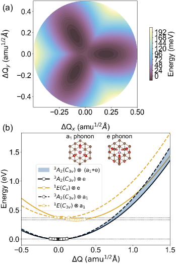
Figure 2: (a) Adiabatic potential energy surface (APES) of $\prescript{1}{}{E}$ of the NV center with the dynamical JT effect. $\Delta Q$ denotes the nuclear coordinate change, the mass weighted total nuclear displacement. $x$ and $y$ represent the displacement directions due to the degenerate $e_{x}$ and $e_{y}$ phonons, respectively. (b) The configuration coordinate diagram for the ${{}^{1}\widetilde{E}}\rightarrow{{}^{3}\widetilde{A}_{2}}$ ISC. The ISC starts from ${{}^{1}\widetilde{E}}$, whose geometry at local energy minima can have $C_{3v}$ and $C_{s}$ symmetries, and ends at ${{}^{3}\widetilde{A}_{2}}$ of $C_{3v}$ symmetry. The solid line represents the potential energy curve created by electron coupling with $e$ phonon, and the dashed line represent that due to electron coupling with $a_{1}$ phonon. The shaded area between the solid and dashed lines include electron coupling with the mix of $a_{1}$ and $e$ phonons. The inset is the visualization of effective $a_{1}$ and $e$ phonons, whose arrows represent the vibration amplitude larger than the threshold $0.05~{}\mathrm{amu}^{1/2}$\mathrm{\SIUnitSymbolAngstrom}$$ and $0.1~{}\mathrm{amu}^{1/2}$\mathrm{\SIUnitSymbolAngstrom}$$, respectively.

III.5 Internal Conversion 

The IC represents spin-conserving phonon-assisted nonradiative transition. Under the static coupling approximation and one-dimensional effective phonon approximation, the equation of nonradiative transition rates is written as in Refs. [66, 22].

$$\begin{split}k_{\text{IC}}&=\frac{2\pi}{\hbar}g|W_{if}|^{2}X_{if}(T)\\ \end{split}$$ (19)

$$\begin{split}W_{if}&=(\varepsilon_{f}-\varepsilon_{i})\innerproduct{\psi_{i}(\mathbf{r,R})}{\frac{\partial\psi_{f}(\mathbf{r,R})}{\partial Q}}\bigg{|}_{\mathbf{R=R_{a}}}\\ \end{split}$$ (20)

$$\begin{split}X_{if}&=\sum_{n,m}p_{in}(T)\Big{|}\matrixelement{\phi_{fm}(\mathbf{R})}{Q-Q_{a}}{\phi_{in}(\mathbf{R})}\Big{|}^{2}\\ &\quad\times\delta(m\hbar\omega_{f}-n\hbar\omega_{i}+\Delta E_{if}).\end{split}$$ (21)

This equation is similar to that of ISC except that the electronic term $W_{if}$ replaces SOC $\lambda$ with single particle wavefunctions $\psi_{i}$ to approximate many-electron wavefunctions, and that the phonon term becomes $X_{if}$ with additional expectation values of nuclear coordinate change ($Q-Q_{a}$).

From our calculations reported in Table 4, $\prescript{3}{}{E}\rightarrow\prescript{3}{}{A}_{2}$ shows long IC lifetime (${\gg}1$ s) because a great number of emitted phonons is needed to fulfill the energy conservation between $\prescript{3}{}{E}$ and $\prescript{3}{}{A}_{2}$. Therefore, this process is a radiative-dominant process. On the other hand, the $\prescript{1}{}{A}_{1}\rightarrow\prescript{1}{}{E}$ transition is likely to be nonradiative-dominant according to past experiments [50], but does not appear in the calculation where we obtain long IC lifetime. This could be a consequence of inaccurate description of the electron-phonon coupling of multi-reference states $\prescript{1}{}{A}_{1}$ and $\prescript{1}{}{E}$, currently calculated at DFT.

Although the calculated IC rate of $\prescript{1}{}{A}_{1}\rightarrow\prescript{1}{}{E}$ is underestimated, we can correct the IC rate. We estimate $W_{if}$ and $X_{if}$ by considering the pseudo JT-induced state mixing coefficients of ${{}^{1}\widetilde{E}}$ and ${{}^{1}\widetilde{A}_{1}}$, and the experimental Huang-Rhys factor [15, 63, 69, 70, 22]. The detailed procedure can be found in SM Sec. V C. With the corrected $W_{if}$ and $X_{if}$, the $k_{\text{IC}}({{}^{1}\widetilde{A}_{1}}\rightarrow{{}^{1}\widetilde{E}})$ can be enhanced by orders of magnitude and closer to experiment, as can be seen in Table 4.

Without correcting the IC rate, we find that the PL rate ($k_{\text{PL}}=k_{\text{R}}+k_{\text{IC}}$) of $\prescript{1}{}{A}_{1}\rightarrow\prescript{1}{}{E}$ is underestimated, but still allows us to obtain qualitatively correct ODMR contrast. When we consider the corrected $k_{\text{IC}}({{}^{1}\widetilde{A}_{1}}\rightarrow{{}^{1}\widetilde{E}})$, this transition becomes dominant by nonradiative recombination, and ODMR contrast is in better agreement with experiments. More details can be seen in Sec. III.6.

Table 4: Calculation details of internal conversion of the NV center at 300 K. The degree of geometry degeneracy $g$ is specified as 3. The ZPL is the energy change in the complete nonradiative process. $\Delta Q$ denotes the nuclear coordinate change between the initial and final states. $\hbar\omega_{f}$ is the phonon energy of the final state. $S_{f}=\omega\Delta Q^{2}/2\hbar$ denotes the Huang-Rhys factor under 1D effective phonon approximation. $W_{if}$ and $X_{if}$ are the electronic and phonon terms, respectively.

Transition	ZPL	$\Delta Q$	$\hbar\omega_{f}$	$S_{f}$	$W_{if}$	$X_{if}$	$\tau_{\mathrm{IC}}$	$k_{\mathrm{IC}}$
	(eV)	(amu${}^{1/2}$\mathrm{\SIUnitSymbolAngstrom}$$)	(meV)		(eV/(amu${}^{1/2}$\mathrm{\SIUnitSymbolAngstrom}$$))	(amu$\cdot$\mathrm{\SIUnitSymbolAngstrom}$^{2}$/eV)		(MHz)
$\prescript{3}{}{E}\rightarrow\prescript{3}{}{A}_{2}$	1.95	0.65	67.7	3.38	16.6	$3.17\times 10^{-19}$	${\sim}1$ s	${\ll}1$
$\prescript{1}{}{A}_{1}\rightarrow\prescript{1}{}{E}$ (w/o corr.)	1.13	0.22	76.4	0.46	$5.48*10^{-4}$	$8.84*10^{-12}$	${\gg}1$ s	${\ll}1$
${{}^{1}\widetilde{A}_{1}}\rightarrow{{}^{1}\widetilde{E}}$ (w/ corr.)	1.13	0.33	76.4	0.9	${\sim}1$	$4.19*10^{-10}$	83.2 ns	12.0
$\prescript{1}{}{A}_{1}\rightarrow\prescript{1}{}{E}$ (Expt.)	1.19	0.34	64 [45]	0.9 [45]	–	–	0.9 ns [49]	$1.11\times 10^{3}$  [49]

III.6 Angle-Dependent and Magnetic-Field Dependent ODMR 

The rates of radiative recombination, internal conversion and intersystem crossing obtained from the calculations above set the prerequisite for the simulation of ODMR contrast (spin-dependent PL contrast). Additionally, the ZFS of triplet ground state and excited state are entered to account for their spin sublevels. Our calculated ZFS of $\prescript{3}{}{A}_{2}$ is $D=3.03$ GHz, similar to the experimental value $D=2.87$ GHz [16, 11, 71]. We currently use the experimental value of $D=1.42$ GHz for excited triplet state $\prescript{3}{}{E}$ [71] given methods for accurate prediction of excited state ZFS remain to be developed. The optical saturation parameter $\beta$ and Rabi frequency $\Omega$ are entered as parameters into the model, and their values are selected within the experimental range [43]. cw-ODMR, which is evaluated at the steady state when the populations no longer change as a function of time, is independent on the initial spin state. We then apply an oscillatory microwave field to drive the population between $\ket{-1}$ and $\ket{0}$ spin sublevels in $\prescript{3}{}{A}_{2}$.

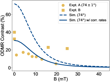
Figure 3: ODMR contrast from the simulation using the calculated rates compared with Expt. A [11] and Expt. B [72]. The angle refers to the angle of magnetic field with respect to the NV axis along [111]. Expt. A shows an angle of $74\pm 1$$\mathrm{\SIUnitSymbolDegree}$. The angle of magnetic field in Expt. B is unknown. The dashed blue curve is the ODMR simulation using all the rates from calculations. The solid blue curve is the simulation with calculated rates and corrected $k_{\perp/z}(\prescript{1}{}{E}\rightarrow\prescript{3}{}{A}_{2})$ and $k_{\text{IC}}(\prescript{1}{}{A}_{1}\rightarrow\prescript{1}{}{E})$ as discussed in Sec. III.4 and Sec. III.5.

Using the input from our first-principles calculations, we plot the simulated ODMR contrast against magnetic field in comparison with the experiments [11, 72] in Fig. 3. The simulated ODMR contrast decreases with increasing the magnetic field, consistent with the trend shown by the experiments (orange dots and squares). Such decrease of ODMR contrast is originated from the mixing of the spin sublevels under magnetic field, as can be seen in SM Fig. S11. The mixing of the spin sublevels leads to smaller contrast of the axial and nonaxial ISC rates, especially $k_{\perp/z}({{}^{3}\widetilde{E}}\rightarrow{{}^{1}\widetilde{A}_{1}})$. Consequently, the spin polarization is less pronounced, manifesting as reduced ODMR contrast.

Our simulated ODMR contrast is overestimated compared to experiments. This is because of the underestimated ISC rates $k_{\perp/z}({{}^{1}\widetilde{E}}\rightarrow{{}^{3}\widetilde{A}_{2}})$ and IC rate $k_{\text{IC}}({{}^{1}\widetilde{A}_{1}}\rightarrow{{}^{1}\widetilde{E}})$, with detailed explanation in earlier sections. Under continuous optical excitation, the system is easier to populate ${{}^{1}\widetilde{E}}$ and ${{}^{1}\widetilde{A}_{1}}$ through the channel ${{}^{3}\widetilde{E}}^{\pm 1}\rightarrow{{}^{1}\widetilde{A}_{1}}\rightarrow{{}^{1}\widetilde{E}}$ when there is an applied microwave field driving populations from spin sublevel $\ket{0}$ to $\ket{-1}$. When $k_{\perp/z}({{}^{1}\widetilde{E}}\rightarrow{{}^{3}\widetilde{A}_{2}})$ and $k_{\text{IC}}({{}^{1}\widetilde{A}_{1}}\rightarrow{{}^{1}\widetilde{E}})$ are underestimated, the population accumulates at the singlet states ${{}^{1}\widetilde{A}_{1}}$ and ${{}^{1}\widetilde{E}}$. This results in the enhanced PL intensity contrast between the two situations, namely in the presence and absence of a microwave field. With the corrected rates discussed in Sec. III.5 and Sec. III.4, we obtain ODMR contrast in better agreement with the experiments.

Finally, we study the ODMR contrast dependence on the magnetic field direction. How spin sublevels mix depends on the magnetic field direction with respect to the NV axis, which is quantified by polar angle $\theta$. In Figs. 4(a) and 4(b), we show both the angle dependency and magnetic-field dependency of normalized PL intensity and ODMR contrast. The simulated normalized PL intensity at $\theta=1$\mathrm{\SIUnitSymbolDegree}$$ exhibits similar sharp reduction character as the experiment [73]. This reduction shares the same origin as the ODMR, as elaborated below. When the magnetic field is perfectly aligned with the NV axis, the ODMR contrast is maximal since there is no spin mixing. When magnetic field is slightly misaligned to the NV axis, we can see two positions of sharp reductions of the ODMR contrast at $B={\sim}50$ mT and ${\sim}100$ mT, which are related to the ZFS in $\prescript{3}{}{E}$ and the one in $\prescript{3}{}{A}_{2}$, respectively. This is resulted from the excited state level-anticrossing (ESLAC) and the ground-state level-anticrossing (GSLAC). As can be seen in SM Fig. S11 that shows the extend to which the spin sublevels mix, there is strong spin mixing of $\ket{0}$ to $\ket{-1}$ at ESLAC and GSLAC. When the magnetic field is more misaligned with the NV axis, i.e. $10$\mathrm{\SIUnitSymbolDegree}$<\theta<90$\mathrm{\SIUnitSymbolDegree}$$, the ODMR contrast becomes highly sensitive to the magnetic field, nearly vanishing after the ESLAC. In addition, we find that the GSLAC and ESLAC of the NV center gradually disappear with increasing magnetic field after $B>25$ mT. The vanishing GSLAC and ESLAC can also be reflected by the ODMR frequency plots in SM Fig. S11. In general, this result suggests our theory can reliably predict the ODMR dependence on magnetic field direction, which is useful for setting up experiments.

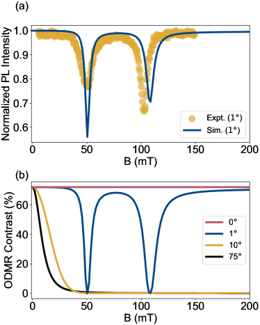
Figure 4: (a) Normalized PL intensity simulated using calculated rates against the applied magnetic field $\mathbf{B}$ whose direction is $1$\mathrm{\SIUnitSymbolDegree}$$ relative to the NV axis. The experiment for comparison is from Ref. [73]. (b) ODMR contrast against magnetic field of an angle with respect to the NV axis [111], which is the spin quantization axis at $B=0$. The strong magnetic field dependency is originated from spin mixing. In both the normalized PL intensity and ODMR contrast, the sharp reduction at $B={\sim}50$ and ${\sim}100$ mT corresponds to level-anticrossing (LAC) in the excited state $\prescript{3}{}{E}$ and ground state $\prescript{3}{}{A}_{2}$, respectively. $B={\sim}50$ and ${\sim}100$ are related to the ZFS in $\prescript{3}{}{E}$ and $\prescript{3}{}{A}_{2}$, respectively. At $\theta=0$\mathrm{\SIUnitSymbolDegree}$$, the ODMR contrast is optimized with no spin mixing.

III.7 Optimization for ODMR Contrast

The optimization of ODMR contrast is a critical step experimentally, as we show next can be realized through tuning optical saturation parameter $\beta$ (related to excitation efficiency $\beta k_{R}$) and tuning Rabi frequency $k_{\text{MW}}$ [43]. Such parameters are cumbersome to search for experimentally but our theory can be much more efficient.

In Fig. 5, we show the optimization of ODMR through the two methods, separately. By Fig. 5(a), we find that ODMR contrast is optimized when the optical excitation power is ${\sim 0.1}$ of the saturation. The part in $\beta>0.1$ is consistent with the experiment [43], and we additionally show the part in $\beta<0.1$, which might be difficult to measure due to low PL intensity under weak optical excitation. Fig. 5(b) indicates that the ODMR contrast can reach its maximum at $k_{\text{MW}}\approx 5$ MHz. When the populations of the spin sublevels are driven by the Rabi oscillation, the nonaxial ISC ${{}^{3}\widetilde{E}}\rightarrow{{}^{1}\widetilde{A}_{1}}$ becomes the preferential path for the relaxation from ${{}^{3}\widetilde{E}}$. Thus, the upper bound of the ODMR contrast in this case is limited by the contrast between $k_{\perp}({{}^{3}\widetilde{E}}\rightarrow{{}^{1}\widetilde{A}_{1}})$ and $k_{z}({{}^{3}\widetilde{E}}\rightarrow{{}^{1}\widetilde{A}_{1}})$.

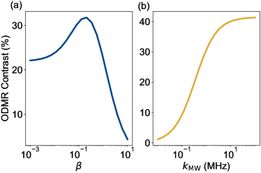
Figure 5: ODMR contrast can be comptimized by tuning (a) optical saturation parameter $\beta$ and (b) Rabi frequency $k_{\text{MW}}$. The ODMR is simulated at $B=0$ and $\theta=0$. The corrected rates are used for the ODMR simulation to show the optimization of ODMR contrast.

IV Conclusion

In conclusion, we have developed general first-principles computational platform for spin-dependent PL contrast and cw-ODMR, for triplet and singlet spin defects in solids. We solved the kinetic master equation with excited-state relaxation rates calculated from first-principles. We validated our implementation by comparing with the experimental data on NV center and ST1 defect in diamond.

The ODMR simulation from first principles requires electronic structure of spin defects including spin sublevels due to ZFS, and the rates of all possible transitions including radiative recombination, ISC (spin-flip nonradiative recombination) and IC (spin-conserving nonradiative recombination). Our calculations overall show good agreement with experiments on the protopytical solid-state spin defect, NV center in diamond. The results showcase the rich physics underlying the entire excitation and relaxation cycle. In particular, we identify the coupling of $\prescript{1}{}{E}$ and $\prescript{1}{}{E^{\prime}}$ due to the Coulomb repulsion from CASSCF calculation and group theory, and show the corresponding effect on SOC matrix elements. We complete the derivation and calculation for the effective SOC matrix elements of the NV center considering pseudo JT effect.As a result, we unequivocally clarify the experimental observation of the axial ISC ${{}^{3}\widetilde{E}}\rightarrow{{}^{1}\widetilde{A}_{1}}$, which was thought to be forbidden in the first order by symmetry. Importantly, we show dynamical JT effect in the degenerate states $\prescript{3}{}{E}$ and $\prescript{1}{}{E}$ significantly enhances the nonradiative recombination by reducing the potential energy barrier.

Finally, we simulate cw-ODMR of the NV center from first-principles calculations. We provide the optimization strategies for ODMR contrast with respect to magnetic field, optical saturation parameter and Rabi frequency. These are found to be informative especially for the range of conditions difficult to reach experimentally. This shows the critical role of our computational technique can play in guiding experiments, which also enables deeper understanding to the spin polarization of spin defects.

The study emphasizes the importance of accounting for the multi-reference character of the electronic states, SOC and electron-phonon coupling for spin defects. It unveils the challenge that there is a need of developing advanced first-principles theory for accurate prediction of SOC and electron-phonon coupling in solid-state spin defects. On the other hand, the atomic structure of many spin defects has not been determined yet, such as ST1 defect in diamond and quantum defects in two-dimensional wide-band gap semiconductors. Our developed computational platform can be essential for identifying existing spin defects, and potentially applied to the design of new solid-state spin defect important for nanophotonics and quantum information science.