Escape time in bistable neuronal populations driven by colored synaptic noise
Abstract
Local networks of neurons are nonlinear systems driven by synaptic currents elicited by its own spiking activity and the input received from other brain areas. Synaptic currents are well approximated by correlated Gaussian noise. Besides, the population dynamics of neuronal networks is often found to be multistable, allowing the noise source to induce state transitions. State changes in neuronal systems underlies the way information is encoded and transformed. The characterization of the escape time from metastable states is then a cornerstone to understand how information is processed in the brain. The effects of correlated input forcing bistable systems have been studied for over half a century, nonetheless most results are perturbative or valid only when a separation of time scales is present. Here, we present a novel and exact result holding when the correlation time of the noise source is identical to that of the neural population, hence solving in a very general setting the mean escape time problem.
Recurrent neural networks (RNN) are powerful and widespread models used to study the emergent dynamics of large networks of interacting neurons and their information processing capabilities [1, 2]. The single node dynamics is derived either phenomenologically [3, 4] or by first-principle under mean-field approximation [5, 6, 7, 8, 9]. They generally consist of differential equations for macroscopic quantities that describe the collective behaviour of neuronal populations. A common choice is the population firing rates , i.e. the fraction of neurons that emit spikes per unit of time. The simplest dynamical law for is:
| (1) |
where is the current-to-rate gain function, controls self-excitation, and is the synaptic current afferent to the neural population. is the relaxation time that we set to be the unit measure of time ( in the following).
By bridging micro- and and mesoscopic scales, networks of units like (1) can effectively model brain networks provided that suited connectivity matrices are incorporated. Besides, RNNs are universal approximators of dynamical systems [10], and as such they can mimic any computer algorithm [11, 12]. Given such computational power, it is not surprising with that over time RNNs have been widely used as “reservoir computers” modeling brain functions like storing memories [13, 14] and performing cognitive tasks [15, 16, 2]. Despite the multidisciplinary relevance of this modeling framework, the mechanistic roots of these computational capabilities and their intricate dependency on both network connectivity and single nodes features, is not yet fully understood. Of particular interest is the case of self-coupling for which the neuronal population displays bistability (for the critical value is ). Bistability in local cortical network has been linked with neural information processing and has been found in neuronal data as well [17]. This question prompted us to better understand metastability in these system, in particular the average residence time which will be the main focus of this letter. In fact, first passage times, i.e. the time needed to jump between states due to fluctuations, are of primary importance in statistical physics [18, 19], biology [20], chemistry [21] and many more fields of science. The synaptic current is generally a sum of external stimuli and neuronal activities of other population in the brain. Due to various sources of intrinsic randomness [22] we can assume to be a random process [23]. One of the main source of such noise is the fact that neuronal populations have a finite size (i.e. a finite number of neurons) [6, 24]. Finite-size fluctuations are correlated in time [24, 25]. Besides, such fluctuating activity is non-instantaneously delivered to postsynaptic neurons with a distribution of transmission delays further filtered by a non-instantaneous synaptic transmission. Both these effects can be accurately modeled considering the synaptic current as an Ornstein-Uhlenbeck (OU) process with correlation time [26]. In summary we will study the stochastic system:
| (2) |
where is a standard Gaussian noise (, and ). The synaptic input is an OU process with correlation time , zero mean and asymptotic variance . [26, 27]. As mentioned above, for strong enough self-coupling (i.e, for the example case ), (2) exhibits bistability. Numerous results have been found in the years that allowed to better understand how noise-induced transition are affected by the level of correlation in the noise source [28]. However, most of them rely on perturbative approaches for or . To the best of our knowledge, no exact results have yet been found in the challenging regime where the two time scales are identical, i.e. . Here we show that an exact result exists allowing us to work out the statistical features of the residence times in one of the metastable states, and to discuss how to leverage the newly found result to go beyond the case envisaging possible applications.
The Fokker-Planck operator —
Our starting point is the Fokker-Planck equation associated to (2):
| (3) |
with diffusion coefficient . Since we cannot write the drift as a gradient of a potential , Eq. (3) is in general difficult to solve. To make some progress we perform the following change of variables: and . Using Ito’s lemma the following stochastic differential equations (SDE) result:
| (4) |
For the specific case , such stochastic dynamics simplifies to
| (5) |
where the two variables and are not independent only because they are driven by the same white noise . The associated Fokker-Planck equation is:
| (6) |
with , and . Here we remark that the operator is the generator of the one-dimensional stochastic process
| (7) |
which in what follows we will take as reference process in characterizing the residence times of the original two-dimensional system (2). Despite the fact that in absence of noise () the drift of (6) is the gradient of a potential function of two independent variable, detailed balance is still broken by the mixed derivatives in [29]. However, we have now access to the marginal distributions of both variables under stationary conditions (i.e., ) defined as and . Indeed, due to the natural boundary conditions of the system (i.e., vanishing probability currents and densities for ), by integrating Eq. (6) with , we obtain whose solution is the Gibbs measure:
| (8) |
where is the potential for in Eq. (7).
Dominant eigenvalues of —
Since the introduced transformation of variables in the previous section is linear, the eigenvalues of the original operator with variable and , are the same as the operator in the variable and .
The decay rate is the sum of escape rates from all the minima of the energy landscape [30]. In what follow we will assume, without loss of generality, that is a bistable symmetric potential hence we have that the mean escape time is were is the dominant (closest to zero) eigenvalue of . We can now prove, for arbitrary and the following :
Theorem 1
If with and a real number, then the spectra of and belong also to the spectrum of .
To prove the theorem we will use a pseudo-spectral approach [31], which consists of an expansion of the eigenfunctions of in terms of the pairwise product of the eigenfunctions of and . First, we define:
| (9) |
and we indicate with a tilde the eigenfunctions of the adjoint operators and . The eigenbasis in braket notation is then:
| (10) |
which is orthogonal with respect to the inner product properly normalized such that . Then the operator is isospectral to the infinite matrix:
| (11) |
where the integer indexes and are mapped for convenience to the unique pairs and , respectively. Direct substitution of in Eq. (11) leads to:
where while . Consider now the rows of associated to the states equal to either or for any arbitrary . Then, since both :
for any arbitrary . Hence the rows of have only one non-zero element which implies that the spectra of and are contained in the spectrum of . Indeed, versors with elements are eigenvectors of as . This result is true for any arbitrary well-defined operators and .
In our case we have that and where are the Hermite polynomials [30], while can be either computed numerically, by solving directly the eigenfunctions boundary value problem with the generalized Scharfetter-Gummel method [32] (see 333Julia script for numerical computation of eigenvalues and eigenfunctions can be found in the repository: https://github.com/giav1n/NeuralPopColoredNoise for our implementation in Julia), or using analytical approximations, for the dominant eigenvalue, that involves integrals of [30]. All our conclusion are independent on the specific functional form of the gain function . As case study in this Letter we use the antisymmetric function .
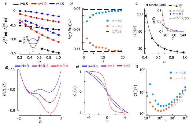
It should be noted that in the spectrum are also present eigenvalues different from and . However two arguments can be made here. First note that, thanks to the property of Hermite polynomial the diagonal of is null (i.e., ), as the partial derivative being . Applying a well know result from eigenvalue perturbation theory we have for the eigenvalues of :
where the versors are the eigenvectors of the diagonal matrix . Consequently, the full spectrum of includes also all the possible sums plus perturbation of order . As depend themselves on , here we are not excluding the possibility that such eigenvalues are not the leading terms of the expansion. Moreover, from a physical point of view, it is typical of multistable systems in regime of small fluctuations to have the first non-null which is a clear manifestation of the separation of time scales induced by the potential barrier that separates different stable states. Since for the one-dimensional -system , as shown inFig. 1a, we conjecture that the dominant eigenvalue of for the full system (2), and thus (4), is precisely . We test this conjecture in numerical simulations. By setting an initial condition of the system relatively close to a stationary and stable solution, a generic expectation value of an arbitrary function follows the exponential decay
where is the expectation value at equilibrium. This asymptotic limit allows to estimate the dominant eigenvalue as
| (12) |
In Fig. 1b the approximations to such limit are shown for the average firing rate , which for sufficiently large remarkably match the of the -system (7) (dashed lines).
In Fig. 1c we show the excellent agreement between the mean escape time of Monte Carlo simulations of system (2) for and . The equivalence of escape statistics between systems (7) and (2) goes beyond the mean as expected for such a separation of time scales eventually leading to a quasi-exponential distribution (Fig. 1c-inset).
Beyond —
When , the synaptic input approaches the white noise limit and the firing rate in Eq. (2)) is no longer an Ito equation because the noise enters nonlinearly in the drift term of . However, in the limit of fast synaptic input , in Eq. (4) and approaches a Wiener process: . Replacing this expression in the SDE (4) for , we eventually obtain the one-dimensional stochastic dynamics
For this systems the mean escape time is given by the inverse of the usual Kramers’ escape rate [19, 30]: with and () is the position of the maximum (minimum) of the potential . Given the scaling rule chosen for the synaptic noise (), in the limit it vanishes and the likelihood to cross the barrier of reduces to 0 as .
In the opposite regime, , we can use the argument presented in [34, 35]. In fact in this case we have that is much faster then and we proceed with an adiabatic approximation. In other words we can assume that reaches its stationary value instantaneously hence, . We can rewrite it as the input needed to reach in a time window smaller than , the asymptotic value :
As shown in Fig. 1d, for small enough , bistability is preserved and no escapes are allowed. A transition deterministically occurs only when the input is larger than a threshold value , i.e., when only one attractor exists, and it is beyond the barrier of the unperturbed system at . Consequently, the escape time in this regime is given by the probability to have in time windows . As fluctuations of have constant variance , the first-passage time needed for such OU process to reach is asymptotically linear in : [36].
Close to we can rely on perturbation theory and the results of this Letter. It is convenient to consider as a small parameter . For arbitrary we can write the Fokker-Planck operator as , where is the operator at and . Following standard perturbation theory of quantum mechanics, we expand eigenfunctions and eigenvalues as , , eventually obtaining for the first-order term in , . Considering from Eq. (10), the only integrals associated to the four terms of differing from 0 are and . From this, the contributing to the longest timescale, is given by the eigenmodes minimizing these two perturbative terms. For the former this happens when , while for the latter when the eigenfunction with the smallest non-zero eigenvalue is taken into account, eventually leading to
| (13) |
The derivative of the mean escape time at is then . Moreover we can demonstrate the following:
Theorem 2
For Fokker-Planck operator , defined in the closed finite interval with continuous drift and diffusion and natural boundary condition in , the integral .
The proof follows form the boundness of the adjoint eigenfunctions (Fig. 1e) 111Since the drift and diffusion are continuous, the adjoint eigenfunctions are continuous as well in the finite interval . The extreme values theorem guarantees the existent of a constant such that . Moreover thanks to the natural boundary condition . Thus . Consequently, for rather general systems, and we can conclude that at least a minimum of must exists and, if we assume that is unique, it must occur for . Note that the existence of optimal value of memory has been reported recently also in the context of active Brownian particle [38, 39, 40] where the noise source acts on the drift of the other variable linearly contrary to the case of neural population dynamics. Thus we have analyzed all possible regimes of correlation time and our prediction are in accordance with Monte-Carlo simulations, see Fig. 1f).
Conclusions —
Most of the result on escape time under the effect of colored noise are derived as effective limit of white noise where the dimensionality of the problem is reduced. On the contrary, our result is exact when the time scales of the two process are identical, , the most unperturbative regime possible. Our conclusions hold for arbitrary value of , and gain function . Moreover, systems like Eq. (2) are rather prototypical dissipative models that have been used in several field of science. For this reason we anticipate that our results might be beneficial also outside the neuroscience domain. Indeed, one possible application of our results is system identification, where the current could be experimentally manipulated and network properties like the level of excitability can be inferred from the escape rate. Another important application can be found in networks of bistable units proven to be successful in performing cognitive tasks [41]. In fact, some of the information processing capabilities of such systems could be deeply linked to the single unit stability to internal noise, which in RNNs with random connectivity naturally arise as chaotic dynamics [42, 43].
Work partially funded by the Italian National Recovery and Resilience Plan (PNRR), M4C2, funded by the European Union - NextGenerationEU (Project IR0000011, CUP B51E22000150006, ‘EBRAINS-Italy’) to M.M.
References
- Sussillo [2014] D. Sussillo, Neural circuits as computational dynamical systems, Curr. Opin. Neurobiol. 25, 156 (2014).
- Vyas et al. [2020] S. Vyas, M. D. Golub, D. Sussillo, and K. V. Shenoy, Computation through Neural Population Dynamics, Annu. Rev. Neurosci. 43, 249 (2020).
- Wilson and Cowan [1972] H. R. Wilson and J. D. Cowan, Excitatory and inhibitory interactions in localized populations of model neurons, Biophys. J. 12, 1 (1972).
- Ostojic and Brunel [2011] S. Ostojic and N. Brunel, From spiking neuron models to linear-nonlinear models, PLoS Comput. Biol. 7, e1001056 (2011).
- Treves [1993] A. Treves, Mean-field analysis of neuronal spike dynamics, Network 4, 259 (1993).
- Brunel and Hakim [1999] N. Brunel and V. Hakim, Fast global oscillations in networks of integrate-and-fire neurons with low firing rates, Neural Comput. 11, 1621 (1999).
- Schaffer et al. [2013] E. S. Schaffer, S. Ostojic, and L. F. Abbott, A Complex-Valued Firing-Rate Model That Approximates the Dynamics of Spiking Networks, PLoS Comput. Biol. 9, e1003301 (2013).
- Montbrió et al. [2015] E. Montbrió, D. Pazó, and A. Roxin, Macroscopic description for networks of spiking neurons, Phys. Rev. X 5, 021028 (2015).
- Mattia [2016] M. Mattia, Low-dimensional firing rate dynamics of spiking neuron networks, arXiv , 1609.08855 (2016), arXiv:1609.08855 .
- Funahashi and Nakamura [1993] K. I. Funahashi and Y. Nakamura, Approximation of dynamical systems by continuous time recurrent neural networks, Neural Netw. 6, 801 (1993).
- Siegelmann and Sontag [1992] H. T. Siegelmann and E. D. Sontag, On the computational power of neural nets, in Proceedings of the Fifth Annual ACM Workshop on Computational Learning Theory (1992) pp. 440–449.
- Koiran et al. [1994] P. Koiran, M. Cosnard, and M. Garzon, Computability with low-dimensional dynamical systems, Theor. Comput. Sci. 132, 113 (1994).
- Cohen and Grossberg [1983] M. A. Cohen and S. Grossberg, Absolute stability of global pattern formation and parallel memory storage by competitive neural networks, IEEE Trans. Syst. Man Cybern. SMC-13, 815 (1983).
- Hopfield [1984] J. J. Hopfield, Neurons with graded response have collective computational properties like those of two-state neurons., Proc. Natl. Acad. Sci. USA 81, 3088 (1984).
- Mastrogiuseppe and Ostojic [2017] F. Mastrogiuseppe and S. Ostojic, Linking connectivity, dynamics and computations in recurrent neural networks, Neuron 99, 609 (2017).
- Yang et al. [2019] G. R. Yang, M. R. Joglekar, H. F. Song, W. T. Newsome, and X.-J. Wang, Task representations in neural networks trained to perform many cognitive tasks, Nat. Neurosci. 22, 297 (2019).
- Brinkman et al. [2022] B. A. W. Brinkman, H. Yan, A. Maffei, I. M. Park, A. Fontanini, J. Wang, and G. La Camera, Metastable dynamics of neural circuits and networks, Appl. Phys. Rev. 9, 011313 (2022).
- Bray et al. [2013] A. J. Bray, S. N. Majumdar, and G. Schehr, Persistence and first-passage properties in nonequilibrium systems, Adv. Phys. 62, 225 (2013).
- Hänggi et al. [1990] P. Hänggi, P. Talkner, and M. Borkovec, Reaction-rate theory: fifty years after Kramers, Rev. Mod. Phys. 62, 251 (1990).
- Codling et al. [2008] E. A. Codling, M. J. Plank, and S. Benhamou, Random walk models in biology, J. R. Soc. Interface. 5, 813 (2008).
- Van Kampen [1992] N. G. Van Kampen, Stochastic processes in physics and chemistry, Vol. 1 (Elsevier, 1992).
- Faisal et al. [2008] A. A. Faisal, L. P. J. Selen, and D. M. Wolpert, Noise in the nervous system, Nat. Rev. Neurosci. 9, 292 (2008).
- Tuckwell [1989] H. C. Tuckwell, Stochastic processes in the neurosciences (SIAM, 1989).
- Mattia and Giudice [2002] M. Mattia and P. D. Giudice, Population dynamics of interacting spiking neurons, Phys. Rev. E 66, 051917 (2002).
- Vinci et al. [2023] G. V. Vinci, R. Benzi, and M. Mattia, Self-consistent stochastic dynamics for finite-size networks of spiking neurons, Phys. Rev. Lett. 130, 097402 (2023).
- Mattia et al. [2019] M. Mattia, M. Biggio, A. Galluzzi, and M. Storace, Dimensional reduction in networks of non-Markovian spiking neurons: Equivalence of synaptic filtering and heterogeneous propagation delays, PLoS Comput. Biol. 15, e1007404 (2019).
- Mattia and Vinci [2021] M. Mattia and G. V. Vinci, Low dimensional dynamics of spiking neuron networks, Zenodo , 5518215 (2021).
- Hänggi and Jung [1995] P. Hänggi and P. Jung, Colored noise in dynamical systems, Adv. Chem. Phys. 89, 239 (1995).
- Deniz and Rotter [2017] T. Deniz and S. Rotter, Solving the two-dimensional fokker-planck equation for strongly correlated neurons., Phys. Rev. E 95, 012412 (2017).
- Risken [1996] H. Risken, The Fokker-Planck Equation, Springer Series in Synergetics (Springer Berlin, Heidelberg, 1996) pp. XIV, 472.
- Shizgal [2015] B. Shizgal, Spectral methods in chemistry and physics, Scientific Computation. Springer (2015).
- Augustin et al. [2017] M. Augustin, J. Ladenbauer, F. Baumann, and K. Obermayer, Low-dimensional spike rate models derived from networks of adaptive integrate-and-fire neurons: comparison and implementation, PLoS Comput. Biol. 13, e1005545 (2017).
- Note [3] Julia script for numerical computation of eigenvalues and eigenfunctions can be found in the repository: https://github.com/giav1n/NeuralPopColoredNoise.
- Moreno-Bote and Parga [2004] R. Moreno-Bote and N. Parga, Role of synaptic filtering on the firing response of simple model neurons., Phys. Rev. Lett. 92, 028102 (2004).
- Woillez et al. [2020] E. Woillez, Y. Kafri, and V. Lecomte, Nonlocal stationary probability distributions and escape rates for an active ornstein-uhlenbeck particle, J. Stat. Mech. 2020, 10.1088/1742-5468/ab7e2e (2020).
- Sato [1977] S. Sato, Evaluation of the first-passage time probability to a square root boundary for the wiener process, J. Appl. Probab. 14, 850 (1977).
- Note [1] Since the drift and diffusion are continuous, the adjoint eigenfunctions are continuous as well in the finite interval . The extreme values theorem guarantees the existent of a constant such that . Moreover thanks to the natural boundary condition . Thus .
- Caprini et al. [2021a] L. Caprini, F. Cecconi, and U. Marini Bettolo Marconi, Correlated escape of active particles across a potential barrier, J. Chem. Phys. 155 (2021a).
- Dabelow et al. [2021] L. Dabelow, S. Bo, and R. Eichhorn, How irreversible are steady-state trajectories of a trapped active particle?, J. Stat. Mech. 2021, 033216 (2021).
- Caprini et al. [2021b] L. Caprini, A. Puglisi, and A. Sarracino, Fluctuation–dissipation relations in active matter systems, Symmetry 13, 81 (2021b).
- Stern et al. [2023] M. Stern, N. Istrate, and L. Mazzucato, A reservoir of timescales emerges in recurrent circuits with heterogeneous neural assemblies, eLife 12, 10.7554/eLife.86552 (2023).
- Sompolinsky et al. [1988] H. Sompolinsky, A. Crisanti, and H. Sommers, Chaos in random neural networks, Phys. Rev. Lett. 61, 259 (1988).
- Stern et al. [2014] M. Stern, H. Sompolinsky, and L. F. Abbott, Dynamics of random neural networks with bistable units, Phys. Rev. E 90, 062710 (2014).