An Oedometer Test under Acid Injection with a Discrete Element Model: the case of Debonding

Abstract

Rock weathering is a common phenomenon in most engineering applications, such as underground storage or geothermal energy. This work offers a discrete element modelization of the problem considering cohesive granular material and debonding effect. Oedometer conditions are applied during the weathering and the evolution of the coefficient of lateral earth pressure, a proxy of the state of stress, is tracked. Especially, the influence of the degree of cementation, the confining pressure, the initial value of $k_{0}$ and the history of load are investigated. It has been emphasized that the granular media aims to reach an attractor configuration. And the grain reorganization occurring is divided into two main phenomena: the collapse of the unstable chain forces (stable only thanks to the cementation) and the softening of the grains.

[1]organization=Institute of Mechanics, Materials and Civil Engineering, UCLouvain, addressline=Place du Levant 1, city=Louvain-la-Neuve, postcode=1348, country=Belgium

[2]organization=Multiphysics Geomechanics Lab, Duke University, addressline=Hudson Hall Annex, Room No. 053A, city=Durham, postcode=27708, country=NC, USA

A bonded granular sample is investigated in oedometer conditions during debonding. The focus is made on the evolution of the $k_{0}=\sigma_{II}/\sigma_{I}$ coefficient, where $\sigma_{I}$ is the stress applied on the vertical surface and $\sigma_{II}$ is the stress applied on the lateral surface.

The existence of an attractor configuration has been emphasized. $k_{0}$ aims to reach the $k_{0}^{attr}$ value.

Two main mechanisms for grain reorganization have been highlighted: the collapse of the unstable chain force (stable only thanks to the cementation) and the softening of the grains.

The influence of several parameters is illustrated, as the cementation, the confining pressure, the load history, and the initial value of $k_{0}$.

1 Introduction

Many rocks are affected by weathering, especially in engineering applications like underground storage [1] or geothermal energy [2]. In particular, underground storage strategies envisioned to store large amounts of $CO_{2}$, captured from large point sources like power generation facilities, or $H_{2}$, produced during overproduction periods of renewable energies like solar or wind, involve the injection of a fluid into a reservoir rock. This fluid reacts with the surrounding rock inducing dissolution and/or precipitation that affects rocks’ permeability [3], but also their mechanical behavior [4]. To ensure the long-term success and safety of such storage solutions, the role of chemo-mechanical couplings needs to be understood and modeled as they can influence settlement at the surface [5, 6], the stability of the caprock [7, 8] or induced seismicity [9].

This weathering has already been investigated experimentally [10, 11, 12] and numerically [13, 14, 15, 16] for rock (bonded material) and sand (unbonded material) in different configurations. Especially, Castellanza and Nova [10] have designed an oedometer test with a soft ring to capture the evolution of the horizontal stress during the debonding phenomena of a rock.

The work presented in this paper pursues this investigation with numerical simulations solved by discrete element modelization. The rock material is described as a cohesive granular material [17]. The mechanical parameters calibrated by Sarkis et al. [18] on biocemented sands [19] have been considered.

Several parameters such as the degree of cementation, the confining pressure, and the history of load are investigated here. Especially, the initial value of the coefficient of lateral earth pressure, a proxy of the state of stress, is monitored and studied. Indeed, this parameter can be affected by tectonic solicitations in the context of underground reservoirs [20, 21, 22] and reaches a larger value than in experimental setups.

The first section of this paper is dedicated to the formulation of the model used in the discrete element modelization. Then, a second one describes the framework and the context of this work. Finally, results and discussions are proposed in the next sections.

2 Theory and formulation

The Discrete Element Model (DEM) is an approach developed by Cundall & Strack [23] to simulate granular materials at the particle level. The foundation of this method is to consider inside the material the individual particles and their interactions explicitly [24]. Newton’s laws (linear and angular momentum) are used to compute the motion of the grains, formulated as follows for one grain:

$$m\frac{\partial v_{i}}{\partial t} =mg_{i}+f_{i}$$ (1)

$$I\frac{\partial\omega_{i}}{\partial t} =M_{i}$$ (2)

where $m$ is the particle mass, $v_{i}$ is the particle velocity vector, $g_{i}$ is the gravity acceleration vector, $f_{i}$ is the sum of contact force vectors applied to the particle, $I$ is the moment of inertia of the particle, $\omega_{i}$ is the angular velocity vector, $M_{i}$ is the sum of contact moment vectors applied to the particle (torques due to bending, and to twisting and to the tangential forces).

Considering two particles with radii $R^{1}$ and $R^{2}$, the interaction between particles is computed only if the distance between grains satisfies the following inequality:

$$\overline{x^{1}_{i}-x^{2}_{i}}<R^{1}+R^{2}$$ (3)

where $x^{1}_{i}$ (resp. $x^{2}_{i}$) is the center of the particle 1 (resp. 2) and $\overline{u_{i}}$ is the norm of the vector $u_{i}$. Once contact is detected between grains $1$ and $2$, the normal vector of the contact $n^{12}_{i}$ is computed as $n_{i}^{12}=(x_{i}^{1}-x_{i}^{2})/\overline{x^{1}_{i}-x^{2}_{i}}$. Then the normal overlap vector $\Delta_{ni}$ and the tangential overlap vector $\Delta_{si}$ are determined.

$$\Delta_{ni}=\left(R^{1}+R^{2}-\left(x_{j}^{1}-x_{j}^{2}\right)n_{j}^{12}\right)n^{12}_{i}$$ (4)

The tangential component $\Delta_{si}$ is computed incrementally, integrating the relative tangential velocity between particles during the contact.

$$\Delta_{si}=\Delta_{si}+v_{si}^{12}\times dt$$ (5)

where $v_{si}^{12}$ is the relative tangential velocity vector defined in Equation 6 and $dt$ is the time step used in the simulation.

$$v_{si}^{12} =v^{12}_{i}-\left(v^{12}_{j}n^{12}_{j}\right)n^{12}_{i}$$ (6)

$$v^{12}_{i} =v_{i}^{1}-v_{i}^{2}+(R^{1}-\delta/2)\epsilon_{ijk}n^{12}_{j}\omega^{1}_{k}$$

$$+(R^{2}-\delta/2)\epsilon_{ijk}n^{12}_{j}\omega^{2}_{k}$$ (7)

where $v^{12}_{i}$ is the relative velocity vector between grains and $\delta=\Delta_{ni}n^{12}_{i}$ is the norm of the normal overlap vector. Notice that the terms $\left(R-\delta/2\right)$ represent the corrected radii at the contact. Here, the angular velocity vectors $\omega_{i}$ of the grains are considered for computing the tangential overlap vector $\Delta_{si}$. As the contact orientation can evolve with time, it is important to update by rotation and scaling the tangential overlap vector $\Delta_{si}^{new}=\Delta_{si}^{old}-\Delta_{sj}^{old}n_{j}^{12}n_{i}^{12}$ and $\overline{\Delta_{si}^{new}}=\overline{\Delta_{si}^{old}}$.

A relative angular velocity vector $\Delta\omega_{i}$ is also needed to compute the twisting and bending behaviors.

$$\Delta\omega_{i}=\omega^{1}_{i}-\omega^{2}_{i}$$ (8)

This relative angular velocity vector $\Delta\omega_{i}$ is divided into a twisting component $\Delta\omega_{ti}$ and into a bending component $\Delta\omega_{bi}$.

$$\Delta\omega_{ti} =\Delta\omega_{j}n^{12}_{j}n^{12}_{i}$$ (9)

$$\Delta\omega_{bi} =\Delta\omega_{i}-\Delta\omega_{ti}$$ (10)

Those relative angular velocity vectors $\Delta\omega_{ti}$ and $\Delta\omega_{bi}$ are used to compute a twisting and a bending relative angular rotation vectors $\Delta\theta_{ti}$ and $\Delta\theta_{bi}$ incrementally.

$$\Delta\theta_{ti} =\Delta\theta_{ti}+\Delta\omega_{ti}\times dt$$ (11)

$$\Delta\omega_{bi} =\Delta\theta_{bi}+\Delta\omega_{bi}\times dt$$ (12)

As the contact orientation can evolve with time, it is important to update by rotation and scaling the twisting and bending relative angular rotation vectors $\Delta\theta_{ki}^{new}=\Delta\theta_{ki}^{old}-\Delta\theta_{kj}^{old}n_{j}^{12}n_{i}^{12}$ and $\overline{\Delta\theta_{ki}^{new}}=\overline{\Delta\theta_{ki}^{old}}$, with $k=t\text{ or }b$.

The contact models between particles obey a cohesive law [17]. Normal, tangential, bending and twisting models are shown in Figure 1 and described in the following.

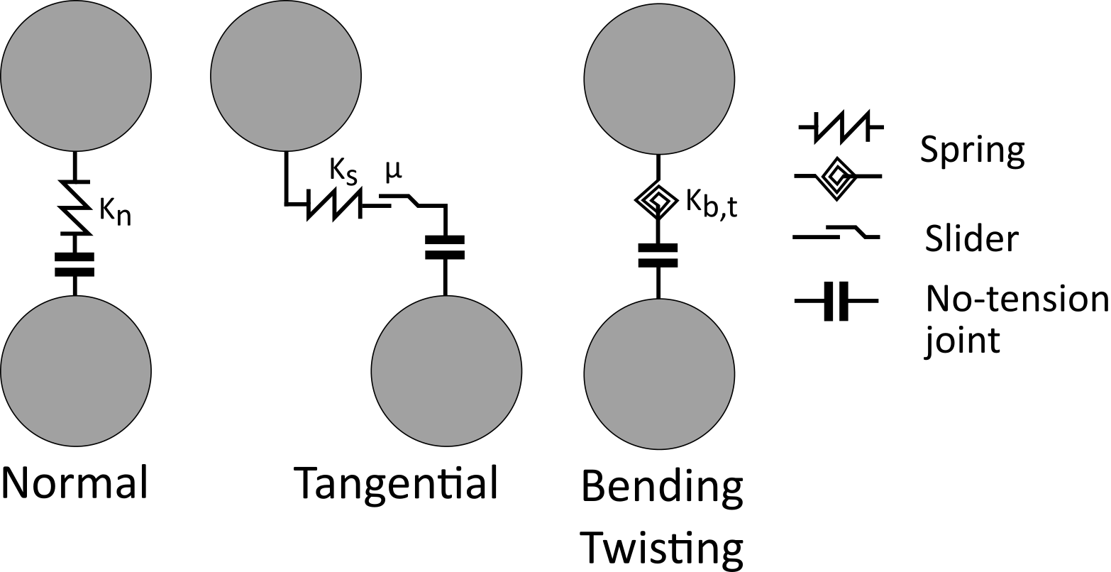
Figure 1: The contact between two particles obeys normal, tangential, bending and twisting elastic-plastic laws. A bond can be present if the contact is cemented. It increases the shear and the tensile strengths.

The normal force vector $F_{ni}$ is described in Equation 13. An elastic stiffness $K_{n}$ is needed, formulated Equation 14.

$$F_{ni} =K_{n}\Delta_{ni}$$ (13)

$$K_{n} =2E_{m}\frac{R^{1}R^{2}}{R^{1}+R^{2}}$$ (14)

where $E_{m}$ is the macroscale Young’s modulus, $R^{1}$ and $R^{2}$ are the radii of the particles in stake.

The tangential force vector $F_{si}$ is described in Equation 15. An elastic stiffness $K_{s}$ is needed, formulated Equation 16.

$$F_{si} =K_{s}\Delta_{si}$$ (15)

$$K_{s} =\nu K_{n}=2\nu E_{m}\frac{R^{1}R^{2}}{R^{1}+R^{2}}$$ (16)

where $\nu$ is the macroscale Poisson’s ratio.

The bending moment vector $M_{bi}$ is described in Equation 17. An elastic stiffness $K_{b}$ is needed, formulated Equation 18.

$$M_{bi} =K_{b}\Delta\theta_{bi}$$ (17)

$$K_{b} =\alpha_{b}K_{s}R^{1}R^{2}=2\alpha_{b}\nu E_{m}\frac{\left(R^{1}R^{2}\right)^{2}}{R^{1}+R^{2}}$$ (18)

where $\alpha_{b}$ is a non-dimensional factor, linking the bending and the tangential stiffnesses.

The twisting moment vector $M_{ti}$ is described in Equation 19. An elastic stiffness $K_{t}$ is needed, formulated Equation 20.

$$M_{ti} =K_{t}\Delta\theta_{ti}$$ (19)

$$K_{t} =\alpha_{t}K_{s}R^{1}R^{2}=2\alpha_{t}\nu E_{m}\frac{\left(R^{1}R^{2}\right)^{2}}{R^{1}+R^{2}}$$ (20)

where $\alpha_{t}$ is a non-dimensional factor, linking the twisting and the tangential stiffnesses. The bending and the twisting resistances aim to reproduce the shape of the grain [25, 26, 27] as spheres are used in this framework (numerically more efficient).

Those contact laws are linear in the elastic domain. Some contact failure is introduced based on the Mohr-Coulomb theory presented in Equation 21.

$$\overline{F_{si}}\leq\mu\;\overline{F_{ni}}$$ (21)

where $\mu$ is the friction coefficient between two particles.

The cementation of the sample is modeled as a cohesion between the grains. The bond exists until one of the two criteria presented in Equation 22 is not verified.

$$\overline{F_{si}} \leq\mu\;\overline{F_{ni}}+\sigma_{s}A_{b}\text{ (Shear condition)}$$

$$\overline{F_{ni}} \leq\sigma_{n}A_{b}\text{ (Tensile condition)}$$ (22)

where $\sigma_{s}$ is the shear strength of the bond, $\sigma_{n}$ is the tensile strength of the bond and $A_{b}$ is the surface of the bond.

3 Numerical model

The initial condition algorithm is presented in Figure 2. A box of $2,8~{}\times~{}2,8~{}\times~{}2,8$ mm is generated. Then $3000$ particles are created. It is important to notice that the grains are initially incorporated with a radius smaller than the final one, as a radius expansion algorithm is applied to generate an initial condition [24]. This algorithm aims to verify a uniform grain size distribution ($R_{min}=75$ $\mu$m and $R_{max}=125$ $\mu$m). Once the particles reach their final dimension, the position of the top wall is controlled to apply a vertical pressure equal to $P_{cementation}$ (see Equation 23 for details). Once the vertical pressure is equal to $P_{cementation}$, the friction between the grains, the twisting resistance and the bending resistance are switched on. Then, the cementation between the particles is done. At every contact, there is a random draw (with a probability equal to $p_{c}$) to determine if a bond is generated. Those bonds verify a shear strength $\sigma_{s}$ and a tensile strength $\sigma_{n}$ and they have a surface $A_{b}$ obtained by a lognormal distribution presented in A and defined by the parameters $m_{log}$ and $s_{log}$ [18]. Once the bonds are generated, the position of the top wall is controlled to apply a vertical pressure equal to $P_{confinement}$ (see Equation 23 for details). It is important to notice that the sample is under oedometer conditions (the control of the top plate aims to verify at any instant the vertical confining pressure) [6, 10]. Then, the position of the lateral wall is controlled to reach an initial coefficient of lateral earth pressure $k_{0}=\frac{\sigma_{II}}{\sigma_{I}}$ ($\sigma_{I}$ is the vertical pressure, $\sigma_{II}$ is the lateral pressure). Once the lateral pressure is verified, the position of the lateral plate is fixed to verify oedometer conditions (fixed lateral walls), and the control of this element is switched off. An example of an initial configuration is illustrated in Figure 3.

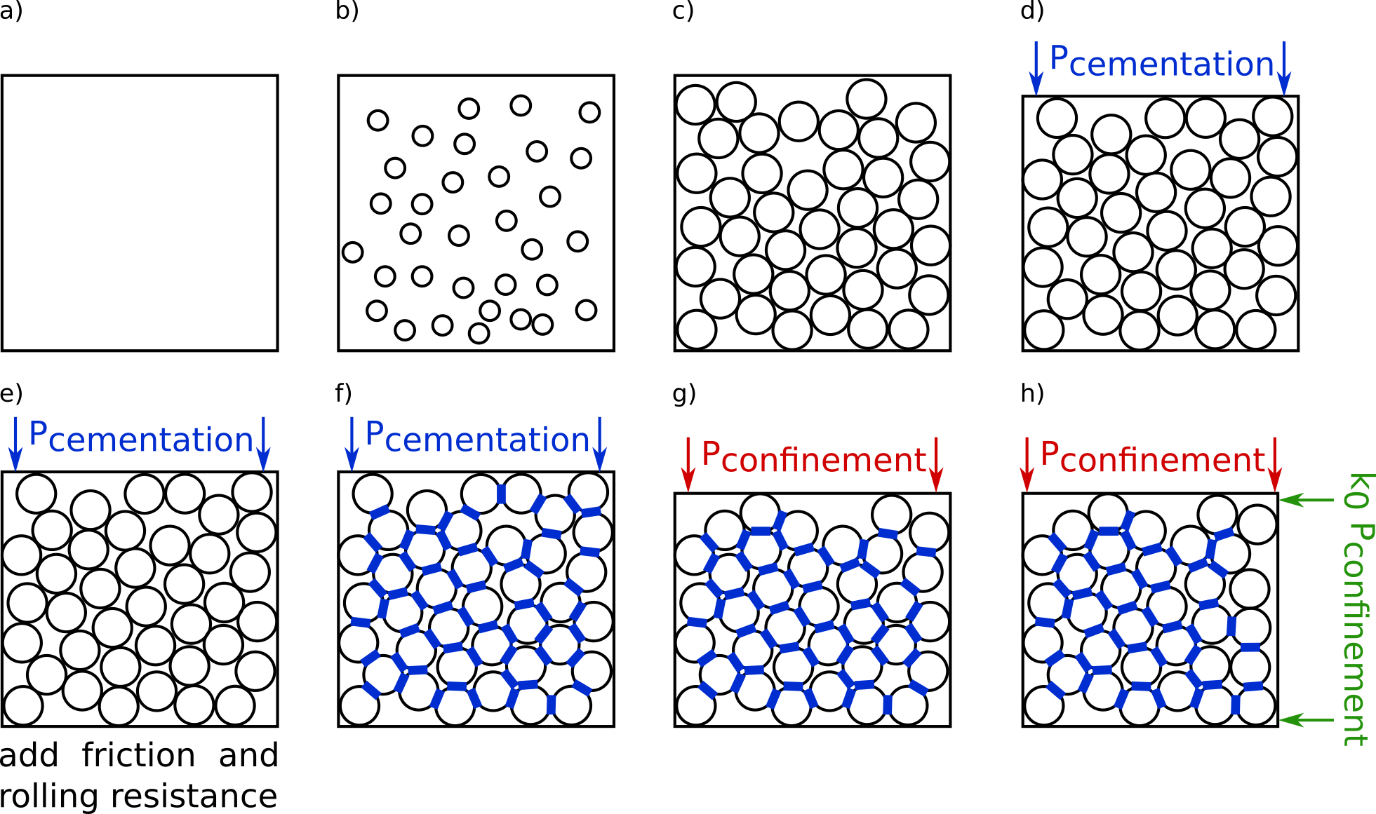
Figure 2: Initial condition algorithm: a) A box is created. b) All the particles are generated with a reduced radius. c) The different radii increase steeply until reaching the final values. d) A vertical pressure is applied by moving the top plate of the box until verifying the vertical pressure $P_{cementation}$. e) The friction, the twisting resistance and the bending resistance are switched on at the contacts. f) The cementation is applied by generating bonds at the contacts. g) A vertical pressure is applied by moving the top plate of the box until verifying the vertical pressure $P_{confinement}$. h) A lateral pressure is applied by moving the lateral plate of the box until verifying the coefficient of lateral earth pressure $k_{0}$.

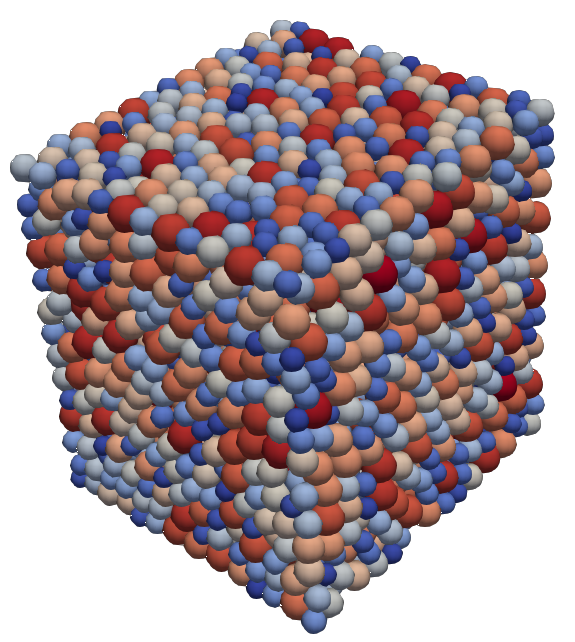
Figure 3: An example of an initial configuration obtained by the algorithm presented in Figure 2. The sample is then in oedometer conditions: the lateral and bottom walls are fixed and a constant vertical pressure is applied at the top.

The control of the wall (top or lateral) is done by a proportional controller $k_{p}$ described in Equation 23. A maximum speed of the plate is applied to verify quasi-static conditions [24].

$$v_{plate} =k_{p}\times\left(P_{plate}-P_{target}\right)$$

$$v_{plate} \leq v_{plate}^{max}$$ (23)

where $v_{plate}$ is the velocity of the plate (in the direction of the control), $k_{p}$ is the value of the proportional controller, $P_{plate}$ is the pressure applied on the plate (in the direction of the control), $P_{target}$ is the targeted pressure applied on the plate (in the direction of the control) and $v_{plate}^{max}$ is the maximum velocity of the plate.

About the walls, no friction, no bending resistance and no twisting resistance are considered with the grains.

Algorithm 1 The weathering of the rock is modelled as a debonding phenomenon.

while Left some bonds do

     Dissolve the bonds $\triangleright$ the bonds surfaces are decreased

     Update the mechanical properties, considering the current cementation

     while not DEM equilibrium do $\triangleright$ granular reorganization occurs

         Compute solicitations

         Solve the momentum balances

         Check the equilibrium criteria for DEM

     end while

     Take a snapshot of the configuration $\triangleright$ Several parameters are tracked

     Count the number of bonds still existing

end while

Once the initial configuration is set, the dissolution steps start. As presented in Algorithm 1, those steps are divided into several parts. First, the bonds are dissolved. The surface of each bond not broken is reduced (the value of the decrease must be small enough to stay representative). Then, the reorganization of the grains occurs until to reach an equilibrium. This state is defined by two characteristics :

• the unbalanced force (defined as the ratio of the mean summary force on bodies and mean force magnitude on interactions) is smaller than a criteria value (here $0.01$).

• the difference between the pressure applied on the top plate and the targeted pressure is smaller than a criteria value (here $0.01\,P_{target}$).

Once the equilibrium is reached a snapshot of the sample is taken. This allows us to track the evolution of different trackers presented in Section 4. Those steps are repeated until all the bonds are broken. Notice that a bond can break because of the dissolution (the surface is null or negative) or because of the loading (criteria presented Equation 22 are reached).

The parameters used in this paper are presented in Tables 1 and 2. The influence of several parameters such as the vertical confinement pressure $P_{confinement}$ [20], the initial coefficient of lateral earth pressure $k_{0}^{init}$ [20, 21, 22] and the degree of cementation [18] are investigated in this paper.

$P_{confinement}$	$0.1$ - $1$ - $10$ MPa
$P_{cementation}$	$0.01P_{confinement}$
Initial $k_{0}$	$0.2$ - $0.7$ - $1.5$
Cementation	2T - 2MB - 11 BB - 13BT - 13MB
Bond dissolution	$0.02\,e^{m_{log}}$ - $0.05\,e^{m_{log}}$ (when $95$ % of the initial number of bonds are broken)

Table 1: Presentation of the parameters used (see Table 2 for the details about the cementation).

		Lightly cemented		Medium cemented	Highly cemented
Sample	Untreated	2T	2MB	11BB	13BT	13MB
Density (kg/m3)	$2650$
$E_{m}$ (MPa)	$80$	$300$	$320$	$760$	$860$	$1000$
$\nu$ (-)	$0.25$
$\alpha_{b}$ (-)	$0.5$
$\alpha_{t}$ (-)	$0.5$
$\mu$ (-)	$0.36$
$p_{c}$ (%)	$0$	$13$	$88$	$98$	$100$	$100$
$m_{log}$ (-)	$0$	$6.79$	$7.69$	$8.01$	$8.44$	$8.77$
$s_{log}$ (-)	$0$	$0.70$	$0.60$	$0.88$	$0.92$	$0.73$
$\sigma_{s}$ (MPa)	$6.6$
$\sigma_{n}$ (MPa)	$2.75$

Table 2: Mechanical parameters depending on the cementation (extracted from [18]).

Looking in Table 2, the Young modulus $E_{m}$ appears to depend on the degree of cementation. An update of the Young modulus (and so, of the different contact springs $K_{n}$, $K_{s}$, $K_{r}$, $K_{t}$) is done during the simulation following Equation 24. The influence of this stiffness reduction will be also investigated in this paper in Section 4.2.

$$E_{m}=(E_{m}^{cementation}-E_{m}^{untreated})\times(1-\xi)+E_{m}^{untreated}$$ (24)

where $E_{m}$ is the current Young modulus used in the simulation, $E_{m}^{cementation}$ is the initial Young modulus depending on the initial degree of cementation, $E_{m}^{untreated}$ is the Young modulus without cementation (here $80$ MPa), and $\xi$ is the debonding factor defined as the ratio of the bonds dissolved (by dissolution or by loading) over the initial number of the bonds.

The time step $dt$ must verify the P-wave critical time step condition [28] defined as:

$$dt<dt_{crit}=\frac{\text{min}(R)}{\sqrt{E_{m}/\rho}}$$ (25)

where $R$ is the radius of the grains, $E_{m}$ is the Young modulus and $\rho$ is the density of the material. Here, a safety factor is considered, $dt=0.6\,dt_{crit}$. As the Young modulus $E_{m}$ evolves with the dissolution of the bonds, an update of this time step $dt$ is also done.

4 Results

The results of this campaign of simulation (plus some complementary investigations) are presented in the following subsections. Two main trackers are used:

• the coefficient of lateral earth pressure $k_{0}=\sigma_{II}/\sigma_{I}$, where $\sigma_{I}$ is the vertical stress and $\sigma_{II}$ is the lateral stress. This parameter is a proxy of the state of stress inside the sample [11, 13].

• the debonding variable $\xi=1-n_{bond}/n_{bond}^{0}$, where $n_{bond}$ is the number of the bond and $n_{bond}^{0}$ is the number of the bond after the initial configuration. This variable is equal to $0$ when the simulation starts (no bond broken) and equal to $1$ when the simulation ends (all bonds broken).

Thanks to the DEM, much more data are available as the coordination number, the mode of rupture of the bonds or the mean force transmitted in the contact, among others. They will be used if necessary.

4.1 The existence of an attractor value $k_{0}^{attr}$

The evolutions of $k_{0}$ are gathered in Figure 4 for all the cementations, the three values of $k_{0}^{init}$ and the different confining pressure $P_{confinement}$.

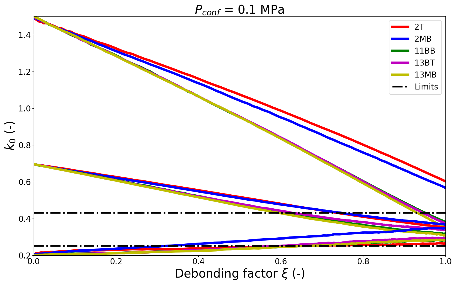
a) b)
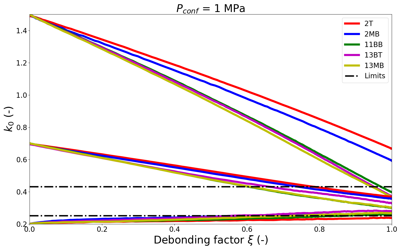
c)

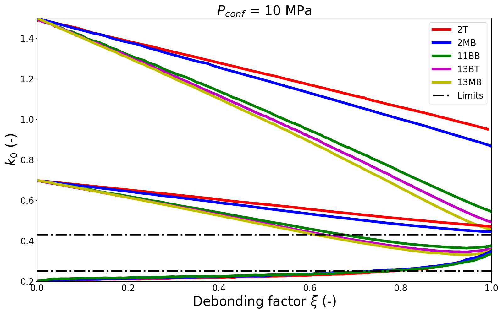
Figure 4: Evolution of $k_{0}$ with the debonding factor $\xi$ for $P_{confinement}=$ a) $0.1$, b) $1$ and c) $10$ MPa. Limits considering $k_{0}^{attr}=\nu/(1-\nu)$ are plotted with $\nu=0.2-0.3$.

It appears the $k_{0}$ aims to reach an attractor value $k_{0}^{attr}$ with the debonding phenomena. This idea of an attractor has already been formulated by Buscarnera and Einav [29] regarding the shape and the size of the grains. Applying the principle of superposition, it has been highlighted that $k_{0}$ approaches a limit given by $k_{0}^{attr}=\nu/(1-\nu)$ during weathering and stiffness reduction [30]. Considering a window of $[0.2-0.3]$ for the value of $\nu$, the attractor value window is $[0.25-0.43]$.

To understand better this phenomenon, the fabric description of the sample and its evolution are investigated. Three simulations are considered: a 13MB sample with a confining pressure $P_{confinement}=1$ MPa and an initial value of $k_{0}=0.2$, $0.4$ or $0.7$. Even if a contact-based fabric tensor is often used in the literature [31, 32, 33], a normal forces-based fabric tensor $F^{n}_{ij}$ [33, 34, 35] is used here. Indeed, the behavior of the grain in the oedometer condition is dominated by the normal forces and the focus is on mechanical anisotropy. The normal forces-based tensor is defined by the average of the outer product of the normal forces at contacts, see Equation 26.

$$F^{n}_{ij}=\frac{1}{N_{c}}\sum\limits_{c}\frac{f^{n}n_{i}n_{j}}{1+D_{kl}n_{k}n_{l}}$$ (26)

where $N_{c}$ is the total number of contacts, $c$ is a contact in the sample, $f^{n}$ is the norm of the normal force of the contact $c$, $n_{i}$ is the unit vector of the contact direction and $D_{kl}$ is the fabric tensor of the second order defined in Equation 27 [33].

$$D_{ij}=\frac{15}{2}\left(\Phi_{ij}-\frac{1}{3}\delta_{ij}\right)$$ (27)

where $\Phi_{ij}$ is the contact-based fabric tensor, defined in Equation 28 [31, 33, 35] and $\delta_{ij}$ is the Kronecker tensor.

$$\Phi_{ij}=\frac{1}{N_{c}}\sum\limits_{c}n_{i}n_{j}$$ (28)

where $N_{c}$ is the total number of contacts, $c$ is a contact in the sample and $n_{i}$ is the unit vector of the contact direction. A distribution function $f^{n}(n_{i})$ can be defined in Equation 29 [33] and illustrated in Figure 5 at initial conditions and at final conditions for $k_{0}^{init}=0.2$, $0.4$ and $0.7$. Even if the initial value of the $k_{0}$ influences the probability distribution function at the initial step, it appears that the fabric aims to reach an attractor configuration thanks to the grain reorganization. This attractor configuration is computed considering the average of the three final configurations.

$$f^{n}(n_{i})=f_{0}\left(1+a^{n}_{ij}n_{i}n_{j}\right)$$ (29)

where $f_{0}=tr(F^{n}_{ij})$ and $a^{n}_{ij}=15/2\left(F^{n}_{ij}/f_{0}-\delta_{ij}\right)$. This function represents the average normal force on a specific direction [34].

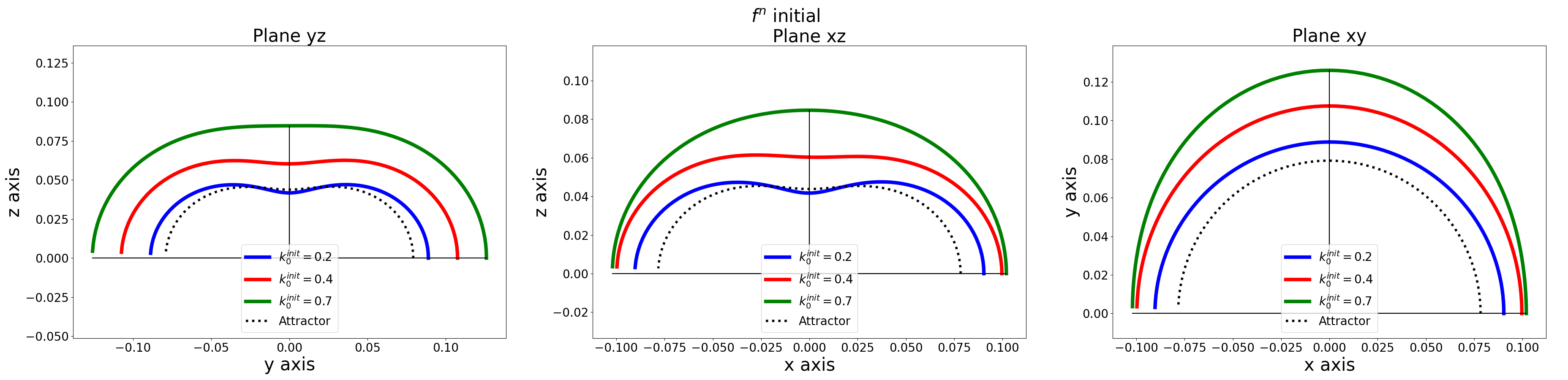
Figure 5: Distribution function $f^{n}(n_{i})$ at initial and attractor conditions.

It appears the $k_{0}^{init}=0.2$ function (blue) is inside the $k_{0}^{init}=0.4$ function (red) which is inside the $k_{0}^{init}=0.7$ function (green). Indeed, it appears in Figure 9, used later in this work, that the mean force transmitted in contact is larger for the case $k_{0}^{init}=0.7$, then for $k_{0}^{init}=0.4$ and finally for $k_{0}^{init}=0.2$. It is in agreement with the definition of the function $f^{n}$. Moreover, it is highlighted that the larger $k_{0}^{init}$ is, the more similar to a circle $f^{n}$ is, for planes yz and xz. The sphericity means that the sample is more isotropic, in agreement with the values of $k_{0}^{init}$ closer to $1$.

One can notice, on plane xy, the fact that an anisotropy exists. Indeed, because of the initial configuration algorithm, see Figure 2, especially the fact that only one wall is moving to apply $k_{0}^{init}$, one loading direction is favorized.

Then, this probability distribution function can be normalized to compare the different organizations. A normalized function $\overline{f^{n}}$ is defined in Equation 30 and shown in Figure 6.

$$\overline{f^{n}}(n_{i})=f_{0}\frac{1+a^{n}_{ij}n_{i}n_{j}}{\int f^{n}\,(n_{i})\,d\theta}$$ (30)

where $\int f^{n}\,(n_{i})\,d\theta$ is the integral of $f_{n}$ along the plane considered (xy, xz or yz). Thanks to this definition, the perimeter of $\overline{f_{n}}$ equals $1$ in the plane. This function represents the probability of a contact to exist in the direction $n_{i}$ weighted by the average normal force in this direction.

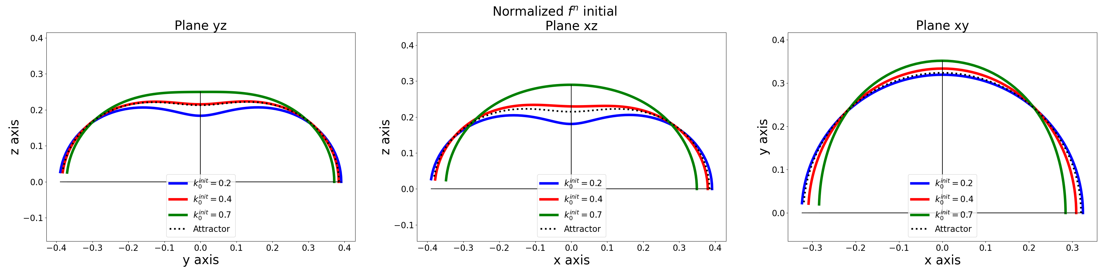
Figure 6: Distribution function $\overline{f^{n}(n_{i})}$ at initial and attractor conditions.

The normalization helps to compare the cases. Looking at planes yz and xz, it is clearer that the $k_{0}^{init}=0.2$ case must create isotropy ($k_{0}$ will increase), whereas the $k_{0}^{init}=0.4$ or $=0.7$ cases must create anisotropy ($k_{0}$ will decrease). The same observations than sooner can be done on the plane xy, one direction is favorized because of the initial condition algorithm, see Figure 2.

The evolution during the debonding of the shape of the normalized probability function $\overline{f^{n}}(n_{i})$ can be captured by the evolution of the maximum and the minimum values, illustrated in Figure 7.

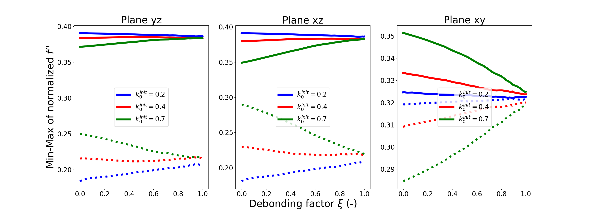
Figure 7: Evolution of the maximum and the minimum values of the normalized probability function $\overline{f^{n}}(n_{i})$ with the debonding factor $\xi$.

It appears that in planes yz and xz, the maximum values increase and the minimum values decrease for cases $k_{0}^{init}=0.4$ and $=0.7$. This distancing of the extrema reveals the creation of anisotropy. On the opposite, the maximum values decrease and the minimum values increase for the case $k_{0}^{init}=0.2$, revealing the creation of isotropy (closing of the extrema). Those observations are in agreement with the evolution of the $k_{0}$ (proxy of the isotropy/anisotropy of the sample). In plane xy, the extrema are closing for the three cases (creation of isotropy). Indeed, the setup presented here does not induce anisotropy on this specific plane. This initial anisotropy is generated by the initial configuration algorithm, see Figure 2.

4.2 Influence of the Young modulus reduction assumption

In this section, the Young modulus reduction assumption, described in Equation 24, is discussed and the $k_{0}$ evolution mechanisms are investigated. The same simulations are run without the Young modulus reduction assumption (the Young modulus stays constant during the debonding of the sample). The results are presented in Figure 8.

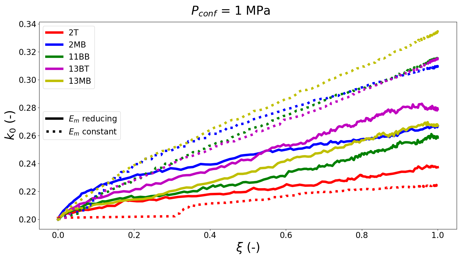
a) b)

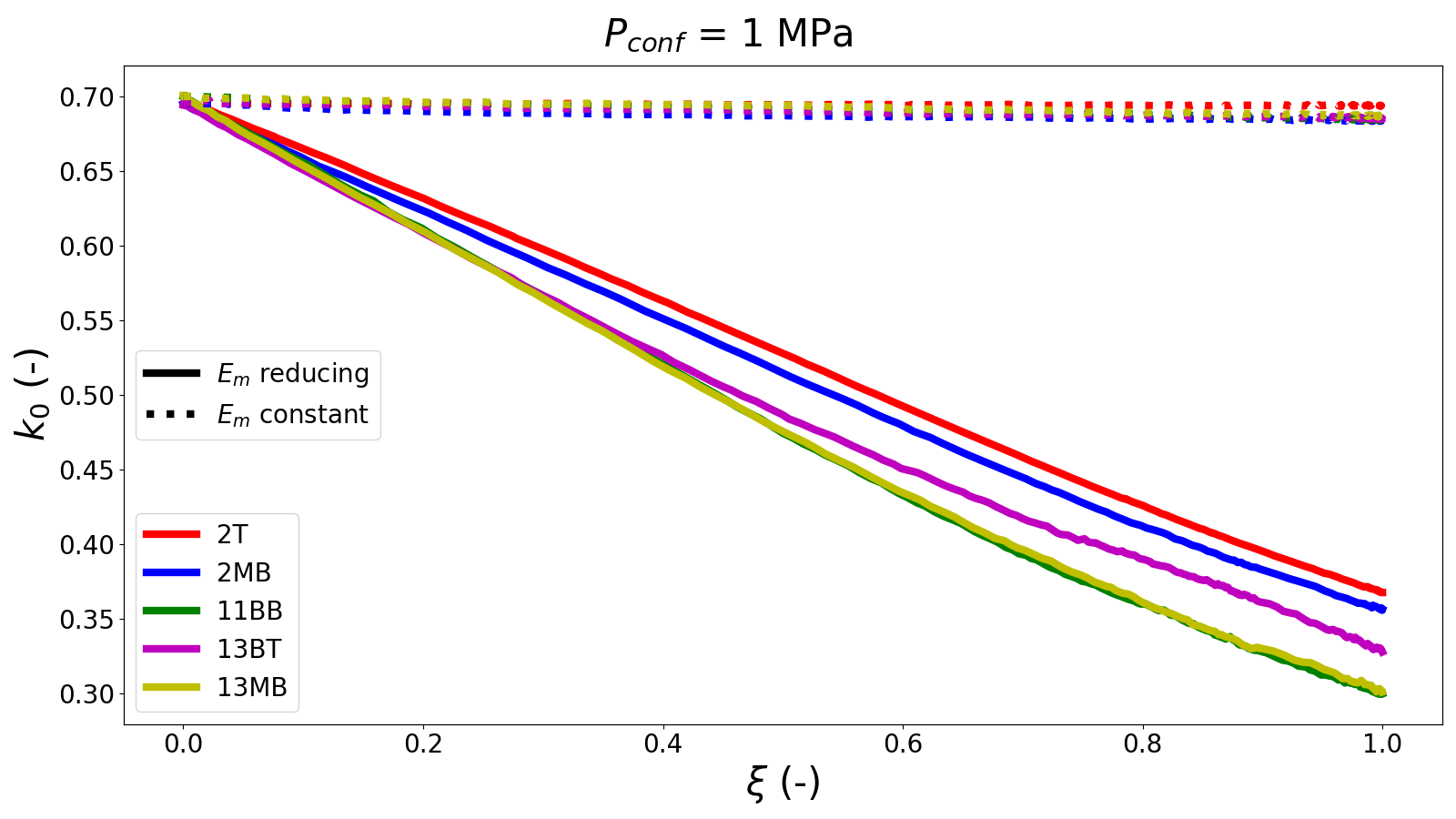
Figure 8: Effect of the Young modulus reduction assumption for different cementations at a confinement pressure $P_{confinement}=1$ MPa with an initial $k_{0}=$ a) $0.2$ or b) $0.7$.

In the case $k_{0}^{init}\leq k_{0}^{attr}$ (here an example with $k_{0}^{init}=0.2$), illustrated in Figure 8a, it appears that a grain reorganization occurs ($k_{0}$ evolves during the dissolution) even if the Young modulus stays constant. It appears in Figure 8b that there is no grain reorganization ($k_{0}$ stays constant during the dissolution) if the Young modulus stays constant and if $k_{0}^{init}\geq k_{0}^{attr}$ (here an example with $k_{0}^{init}=0.7$). In this kind of configuration, the reorganization of the grains is due to the softening of the material (Young modulus reduction). Two mechanisms seem to appear, depending on the state of stress.

This phenomenon is also highlighted by considering the evolution of the mean force and the coordination number (proxy of the grain organization). Three simulations are considered: a 13MB sample with a confining pressure $P_{confinement}=1$ MPa and an initial value of $k_{0}=0.2$, $0.4$ or $0.7$. The results are shown in Figure 9.

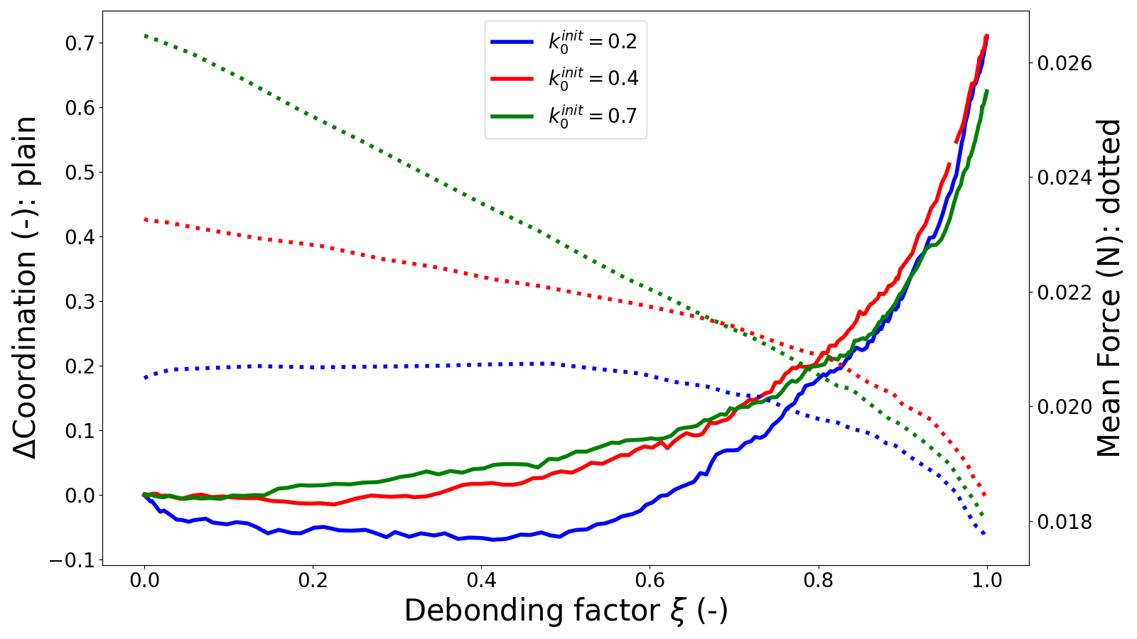
Figure 9: Evolution of the coordination number (plain line), mean number of contacts per grain, with the debonding phenomena. The evolution of the mean force (normal + tangential) transmitted in contacts of the fabric (dotted lines) is plotted in parallel. Notice the coordination number evolutions have been set to start at $0$ to be compared.

The existence of the two mechanisms is emphasized by the fact that the $k_{0}^{init}=0.2$ mean force evolution is different than the $k_{0}^{init}=0.4$ or $=0.7$ mean force evolutions. The first one stays at a constant value ($\approx 0.02$ N) until a threshold value ($\xi\approx 0.6$) for the debonding is reached. The latter decreases linearly from the beginning of the simulation. A second evolution (sharper and less linear) can be spotted after a threshold debonding ($\xi\approx 0.8$). In the same way, it appears the $k_{0}^{init}=0.2$ coordination number aims to reduce at the start of the simulation whereas the $k_{0}^{init}=0.4$ and $=0.7$ coordination numbers increase. This observation reinforced the idea that two mechanisms exist, depending on the state of stress.

4.3 Influence of the initial $k_{0}$ on the grain reorganization mechanism

As emphasized in Section 4.2, the grain reorganization mechanism (evolution of the $k_{0}$) seems to depend on the state of stress. The distribution of the mechanisms of bond rupture presented in Figure 10 emphasizes this phenomenon. The bonds can break in two modes: i) by dissolution (if the bond surface reaches a null or a negative value) or ii) by loading (if criteria presented in Equation 22 are reached). It appears that for the same cementation and the same confining pressure $P_{confinement}$, the percentage of rupture by loading is larger for $k_{0}^{init}\leq k_{0}^{attr}$ than for $k_{0}^{init}\geq k_{0}^{attr}$. To understand this difference, the chain forces are sorted into two kinds: unstable and stable organization. An unstable chain force stays in place thanks to the cementation at the contacts. Once the cement is partially dissolved, the chain force collapses, breaking the reduced but existing cemented contacts. On the opposite, a stable chain force stays in place thanks to the particle-particle contact. If the cemented contacts are dissolved, the chain force does not collapse. Considering $k_{0}^{init}\leq k_{0}^{attr}$, it has been established that grain reorganization occurs only if enough cemented contacts are reduced. Indeed, the unstable chain forces are predominant in this case, see the $k_{0}$ evolution when the Young modulus $E_{m}$ stays constant during the debonding, Figure 8a. Once the cemented contacts are reduced, the cementation at contacts breaks by mechanical loading. Considering $k_{0}^{init}\geq k_{0}^{attr}$, it has been established that grain reorganization occurs directly (no cemented contact reduction is needed). Indeed, the stable chain forces are predominant in this case, see the constant $k_{0}$ when the Young modulus $E_{m}$ stays constant during the debonding, Figure 8b. The cemented contacts break with a chemical rupture as they are not sollicitated.

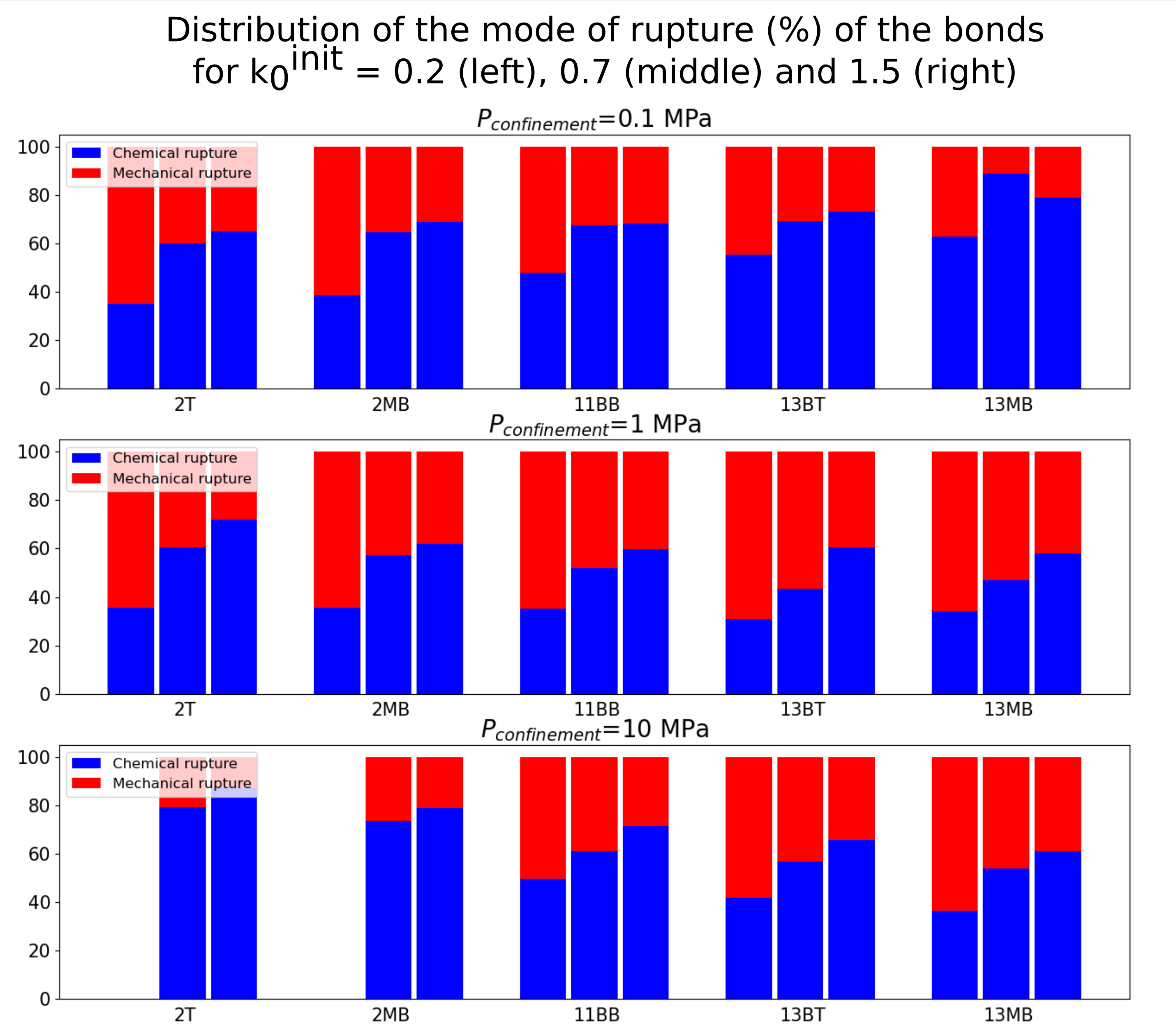
Figure 10: Distribution of the mode of rupture of the bond at the end of the test. A bond can break by chemical dissolution (the bond surface reaches a negative or a null value during the dissolution steps) or by mechanical loading (criteria presented in Equation 22 are reached).

Once the two mechanisms have been described, it is important to notice in the cases of light cementations (2T or 2MB) that the final values of the $k_{0}$ are larger than the others if $k_{0}^{init}\geq k_{0}^{attr}$, see Figure 4. The reduction of the $k_{0}$ is due to the softening of the grains in this case. Considering light cementations, the softening is smaller as the Young modulus evolves only between $300$ MPa (for 2T) or $320$ MPa (for 2MB) and $80$ MPa (for uncemented material) compared to $1000$ MPa (for 13MB), for example. The Young modulus stays around the same value for light cementations and the grain reorganization can not occur. The influence of the initial value of the Young modulus is discussed in Figure 12. It seems the Young modulus has an influence, especially in the case $k_{0}^{init}\geq k_{0}^{attr}$. It appears this influence is smaller in the case $k_{0}^{init}\leq k_{0}^{attr}$.

4.4 Influence of the cementation (different percentage of contacts cemented $p_{c}$, different Young modulus $E_{m}$ and different bond sizes distribution defined by $m_{log}$ and $s_{log}$)

Following the definition of the different degrees of cementation used par Sarkis et al. [18], it appears that the Young modulus $E_{m}$, the percentage of contacts cemented $p_{c}$ and the bond sizes distribution (defined by $m_{log}$ and $s_{log}$) change with the cementation. To understand the effect of the cementation on the problem those three effects must be isolated.

The first aspect to be analyzed is the influence of the percentage of contacts cemented $p_{c}$. This parameter describes the ratio of contact cemented during the initial configuration (see step f in Figure 2) on the total number of contacts. Complementary simulations have been run. An 11BB sample is generated under $P_{confinement}=0.1$ MPa with an initial $k_{0}=0.2$ or $0.7$. Three different values are considered for the parameter $p_{c}=50$, $75$ or $100\%$. The results are presented in Figure 11.

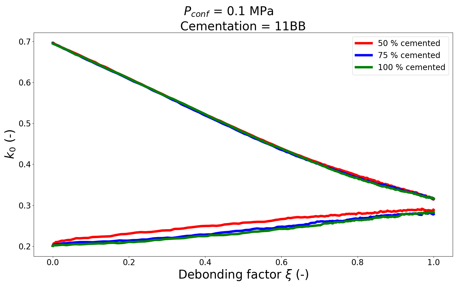
Figure 11: Evolution of the $k_{0}$ with the debonding variable $\xi$ for an 11BB sample under $P_{confinement}=0.1$ MPa with $50$, 75 or $100$% initial contacts cemented.

It appears that $p_{c}$ does not influence the evolution of $k_{0}$. A light difference can be noted for $k_{0}^{init}=0.2$ but it stays negligible compared to the difference noted with the other cementations in Figure 4. This difference can be explained by the fact the reorganization mechanisms are different depending if the initial $k_{0}$ is smaller or larger than the attractor value $k_{0}^{attr}$. As explained in Section 4.3, if $k_{0}^{init}\leq k_{0}^{attr}$ the main reorganization mechanism is the collapses of the unstable chain forces. In this case, the fact that there is less cemented contact ($p_{c}$ smaller) can weaken the global structure and affect lightly the $k_{0}$ evolution. If $k_{0}^{init}\geq k_{0}^{attr}$ the main reorganization mechanism is the grains softening. Here, the distribution of the cemented contact has no influence. To resume, it appears the parameter $p_{c}$ has no influence in the evolution of the $k_{0}$ with the debonding phenomenon.

The second parameter to be analyzed is the Young modulus $E_{m}$. To investigate the effect of this parameter, the same simulations are run but the initial value of the Young modulus can be controlled (considered the same for all cementation: $E_{m}=1$ GPa, Young modulus of the cementation 13MB). The results are shown in Figure 12.

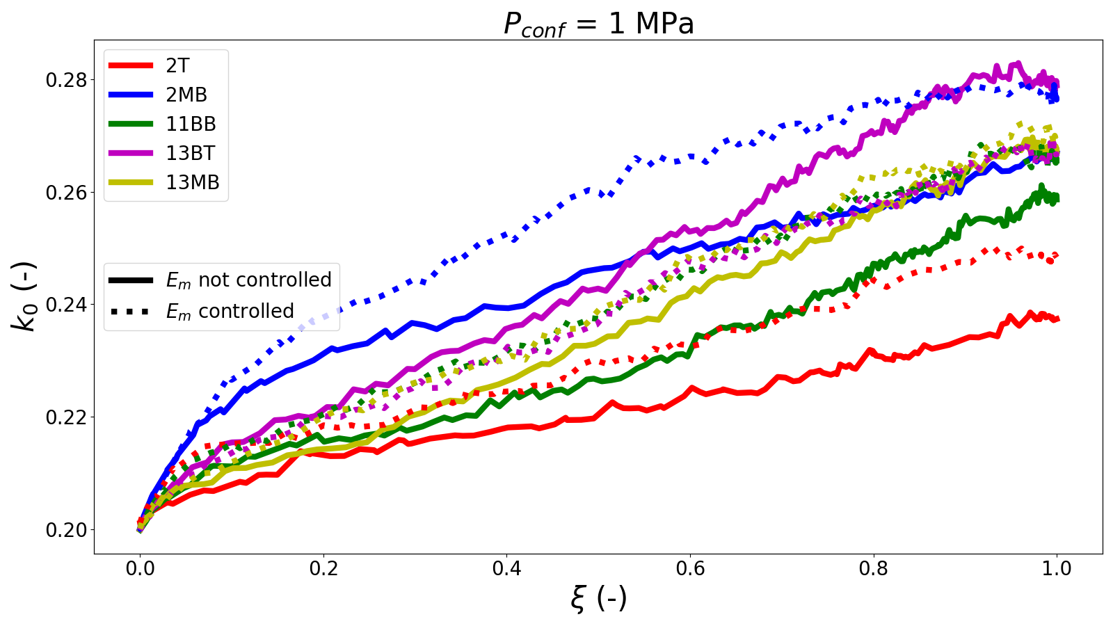
a) b)

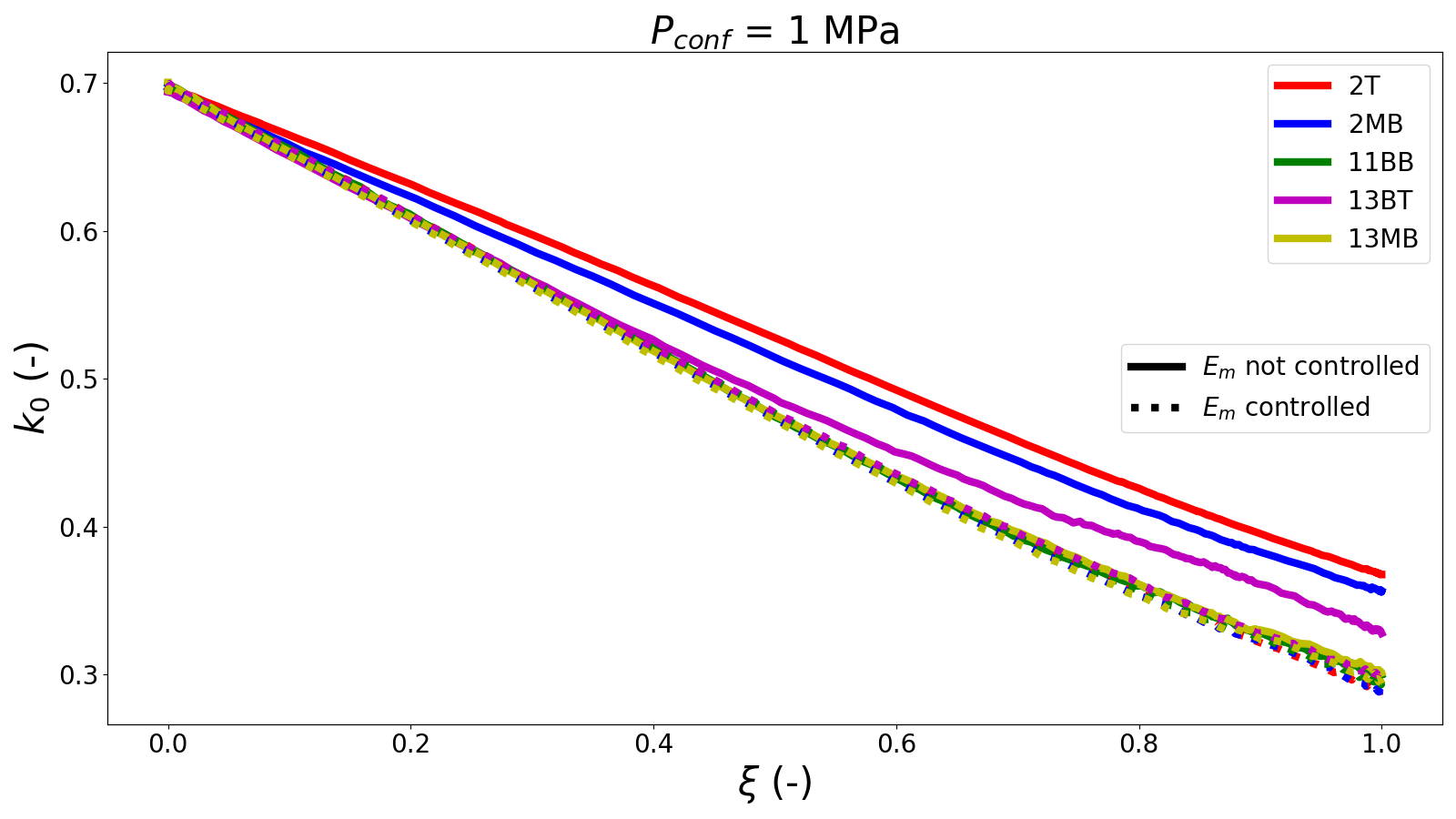
Figure 12: Evolution of the $k_{0}$ with the debonding factor $\xi$ for different cementations at a confinement pressure $P_{confinement}=1e6$ Pa with an initial $k_{0}=$ a) $0.2$ or b) $0.7$. The initial value of the Young modulus $E_{m}$ is equal to $1000$ MPa for the controlled simulations.

For $k_{0}^{init}\leq k_{0}^{attr}$, Figure 12a, it appears the controlled $k_{0}$ evolutions are around the $k_{0}$ evolution obtained with a 13MB cementation (not controlled). This can be understood by the fact the initial Young modulus value is the same as the one used for this cementation. It is important to note that 2T and 2MB controlled simulations give results a bit different. As explained in Section 4.3, the evolution of the $k_{0}$ is more controlled by the unstable chain forces collapses than the softening of the grains for $k_{0}^{init}\leq k_{0}^{attr}$. Lightly cemented samples are composed of fewer bonds between the grains, so the collapse of the chain forces can occur more easily. It seems the initial Young modulus has an influence on the $k_{0}$ evolution but it is not the main one.

For $k_{0}^{init}\geq k_{0}^{attr}$, Figure 12b, it appears the controlled $k_{0}$ evolutions are around the $k_{0}$ evolution obtained with a 13MB cementation (not controlled). This can be understood by the fact the initial Young modulus value is the same as the one used for this cementation. Even the 2T and 2MB controlled simulations give the same results. As explained in Section 4.3, at large initial values the evolution of the $k_{0}$ is more controlled by the softening of the grains than the unstable chain forces collapses. The grain reorganization depends strongly on the initial Young modulus of the grains in the case.

The third parameter to be analyzed is the bond size distribution controlled by $m_{log}$ and $s_{log}$ (see A). It has been emphasized in the previous discussion of this Section that the bond size distribution influences in the case $k_{0}^{init}\leq k_{0}^{attr}$, Figure 12a, and do not in the case $k_{0}^{init}\geq k_{0}^{attr}$, Figure 12b. As presented in Section 4.3, the mechanism of the $k_{0}$ evolution is the collapse of the unstable chain forces. The bond size distribution influences this phenomenon, especially the variance of the distribution $s_{log}$. Moreover, Figure 13 highlights the fact that the light cementations (2T and 2MB) dissolve totally faster than the high cementation (13BT and 13MB). This Figure represents the evolution of the $k_{0}$ with the cumulative bond surface dissolved (similar to the times). Here, the mean of the distribution $m_{log}$ controls the temporal aspect of the debonding phenomena.

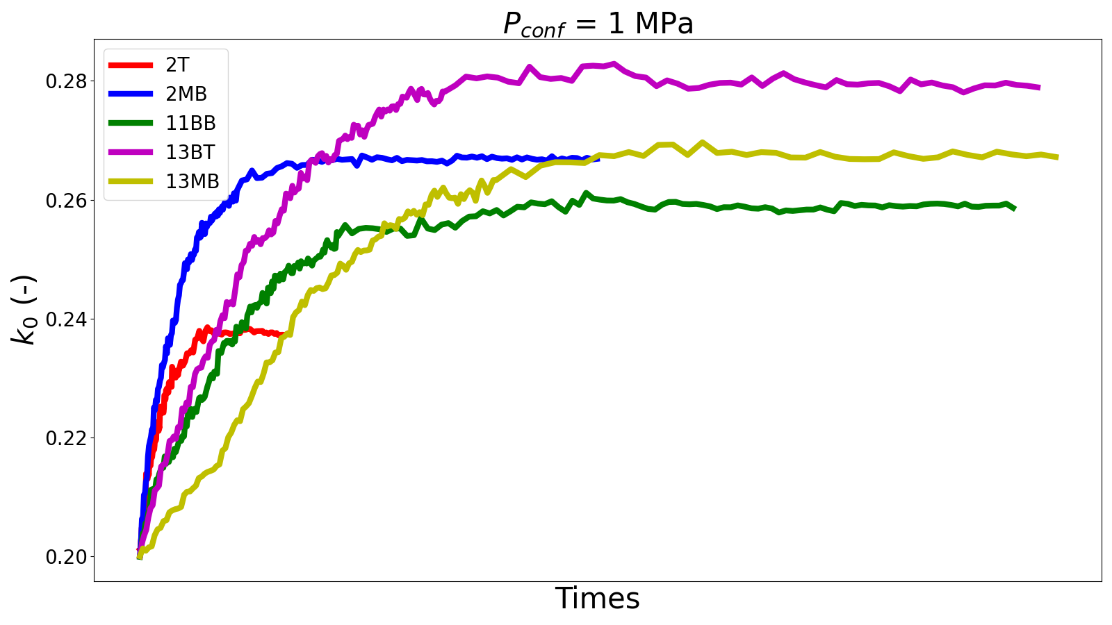
Figure 13: Evolution of the $k_{0}$ with the cumulative bond surface dissolved ($\approx$ the time) for the different cementations at $P_{confinement}=1$ MPa.

4.5 Influence of $P_{confinement}$

The effect of the confinement pressure $P_{confinement}$ is studied in this Section. The results are shown in Figure 14.

a)
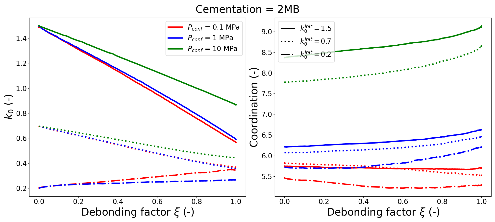
b)
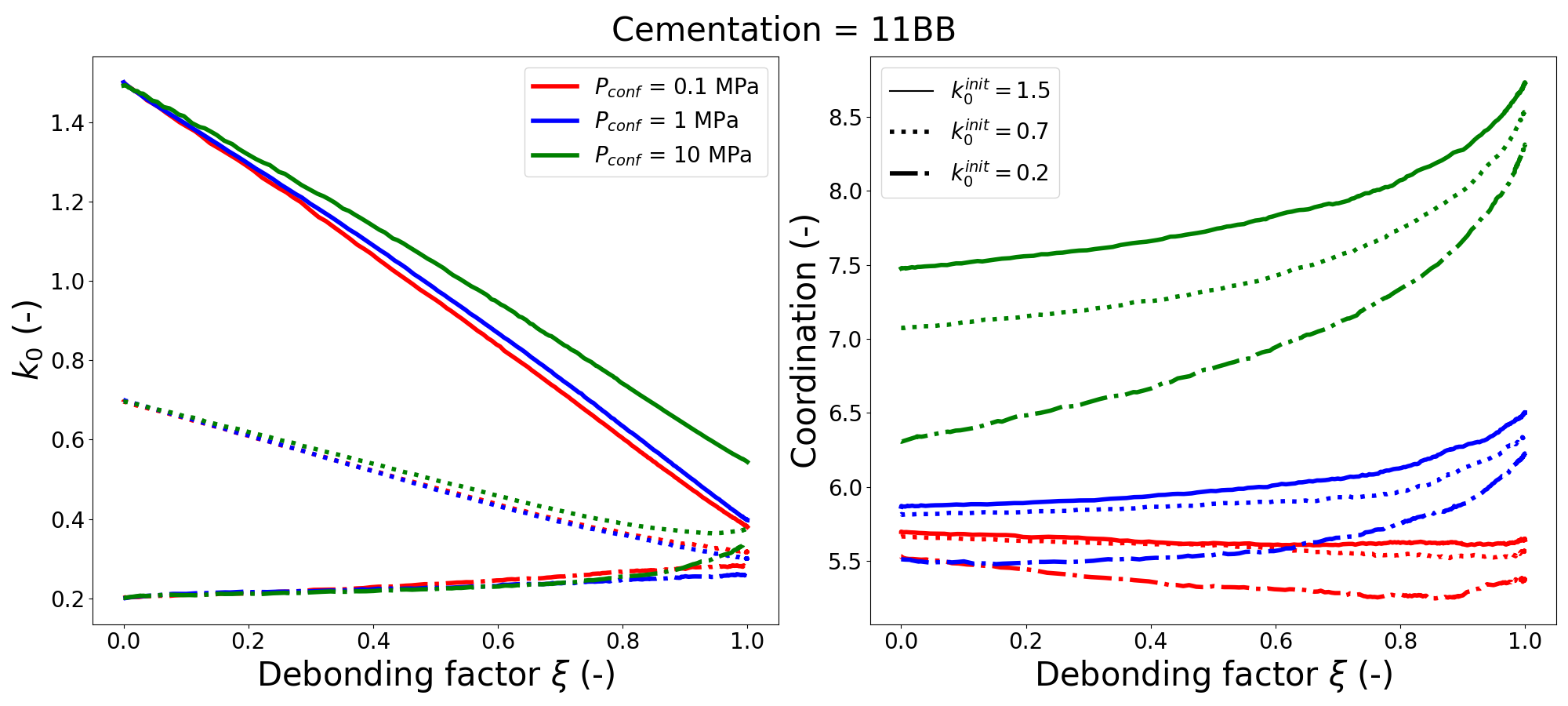
c)

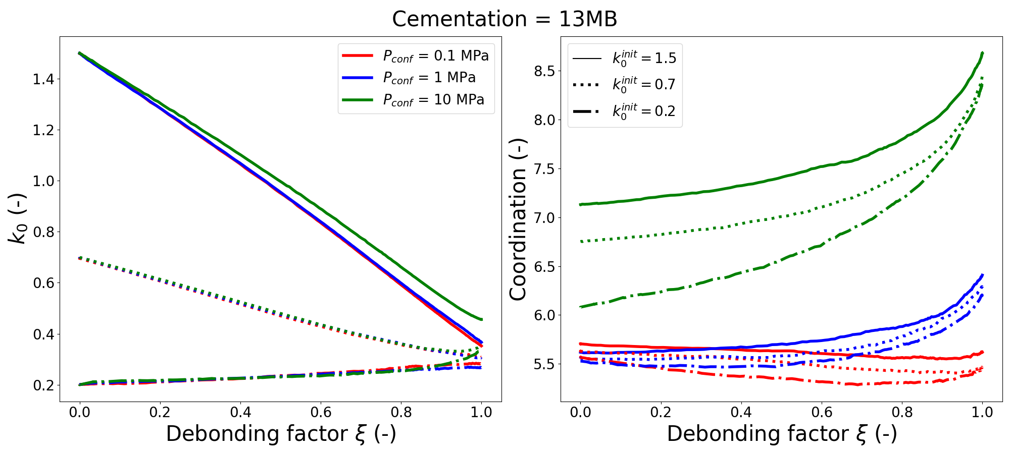
Figure 14: Evolution of the $k_{0}$ and the coordination number with the debonding variable $\xi$ at $P_{confinement}=0.1$, $1$ and $10$ MPa, with $k_{0}^{init}=0.2$, $0.7$ and $1.5$ for three different degrees of cementation: a) 2MB, b) 11BB and c) 13MB.

First of all, it appears that no results are obtained for the light cementations (2T and 2MB) at $P_{confinement}=10$ MPa when $k_{0}^{init}=0.2$. All of the bonds break during the initial configuration set-up as the confinement pressure is large. It is important to notice that the lateral strain $\epsilon_{lat}$ is extensive during the initial set-up for $k_{0}^{init}\leq k_{0}^{attr}$ (aims to reduce $k_{0}$ as this coefficient is around the attractor value at step g of Figure 2) and compressive for $k_{0}^{init}\geq k_{0}^{attr}$ (aims to increase $k_{0}$ as this coefficient is around the attractor value at step g of Figure 2). Because of this extensive mode and the fact that shear failure occurs more, the bonds aim to break more than in the compressive mode.

Figure 14 highlights the fact that the coordination number (the mean number of contacts per grain) increases with $P_{confinement}$. As the confining pressure is larger, the grains are more squeezed and the number of contacts increases. In DEM, this phenomenon must be dealt with carefully, especially for rigid particles. Indeed, the models used are built on the small overlap assumption. This limit is named the jammed state [36]. A new soft particle model has recently been designed to investigate deeper into this jammed state [37]. It appears here that the grain reorganization (see the evolution of the coordination number) is divided into two steps: a linear part at the beginning and a nonlinear part at the end. For a reminder, the Young modulus $E_{m}$ of the grains is decreasing with the debonding and so the sample aims to be closer to the jammed state. As the Young modulus is smaller for small cementations, this state is reached sooner. For example, let’s consider $P_{confinement}=10$ MPa (green lines) and $k_{0}^{init}=1.5$ (plain lines), the nonlinear part starts around $\xi=0.6$ for an 11BB sample and around $\xi=0.7$ for a 13MB sample. In the same idea, for $k_{0}^{init}\geq k_{0}^{attr}$ the final value of the $k_{0}$ is globally larger when $P_{confinement}$ is larger (especially for $P_{confinement}=10$ MPa, green lines). As the sample is closer to the jammed state, there is less space to reorganize. This observation is less clear in the case $k_{0}^{init}\leq k_{0}^{attr}$, as the mechanism of the $k_{0}$ evolution is dominated by the collapse of the unstable chain forces, and not the softening of the grain, see Section 4.3.

5 Discussion

5.1 The evolution of the $k_{0}$ can generate failure

Figure 15 shows the evolution of the $k_{0}$ between the initial and final configurations $\left(\Delta k_{0}=k_{0}^{final}-k_{0}^{initial}\right)$ for different initial $k_{0}^{initial}$ values at different confinement pressures $P_{confinement}$ and for all cementations.

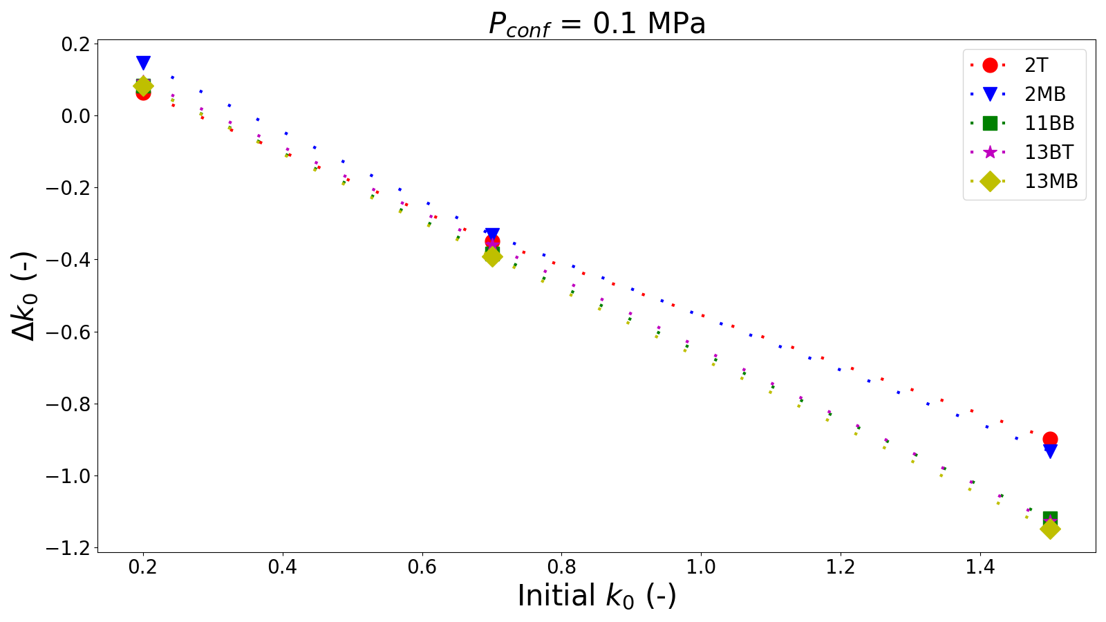
a) b)
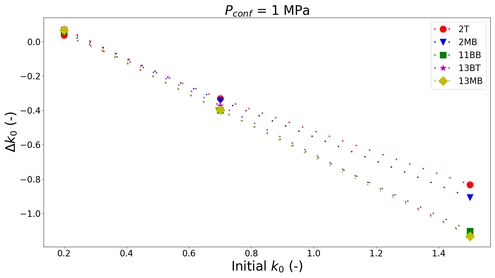
c)

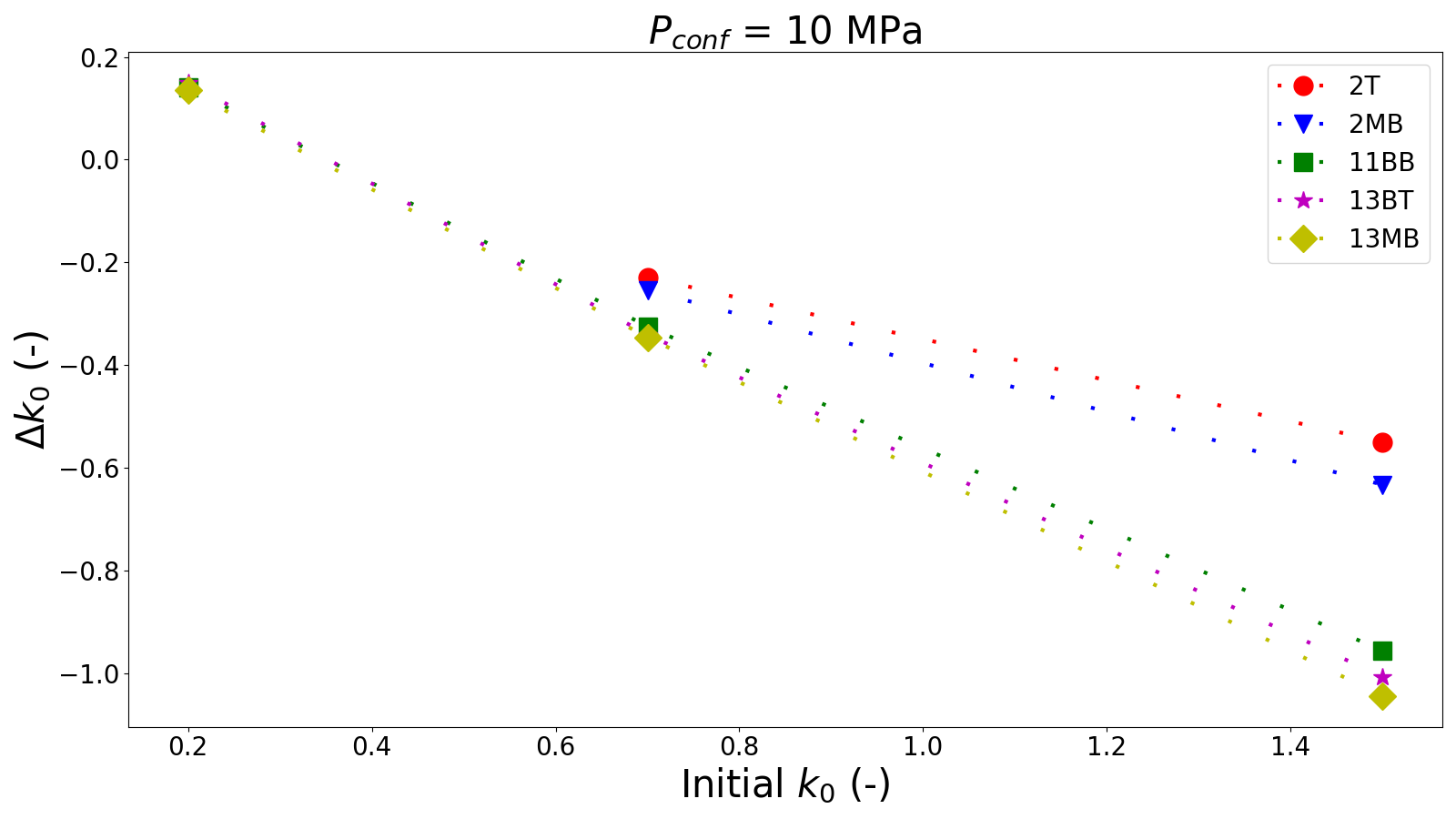
Figure 15: Evolution of the $k_{0}$ between the initial and final configurations $\left(\Delta k_{0}=k_{0}^{final}-k_{0}^{initial}\right)$ for different initial $k_{0}^{initial}$ values and all the cementations at different confinement pressures $P_{confinement}=$ a) $0.1$ MPa b) $1$ MPa or c) $10$ MPa.

This evolution of the $k_{0}$ is really important, especially in the context of an underground reservoir. The host rock can be modelled with a simple Mohr-Coulomb criteria, illustrated in Figure 16. It appears that a reduction of $k_{0}\left(=\sigma_{II}/\sigma_{I}\right)$ aims to induce a failure as the diameter of the Mohr circle increases $\left(D_{MC}=\sigma_{I}\left(1-k_{0}\right)\right)$, where $D_{MC}$ is the diameter of the Mohr circle and $\sigma_{I}$ is the vertical stress. As shown earlier in this work, this $k_{0}$ reduction appears only if $k_{0}^{init}\geq k_{0}^{attr}$.

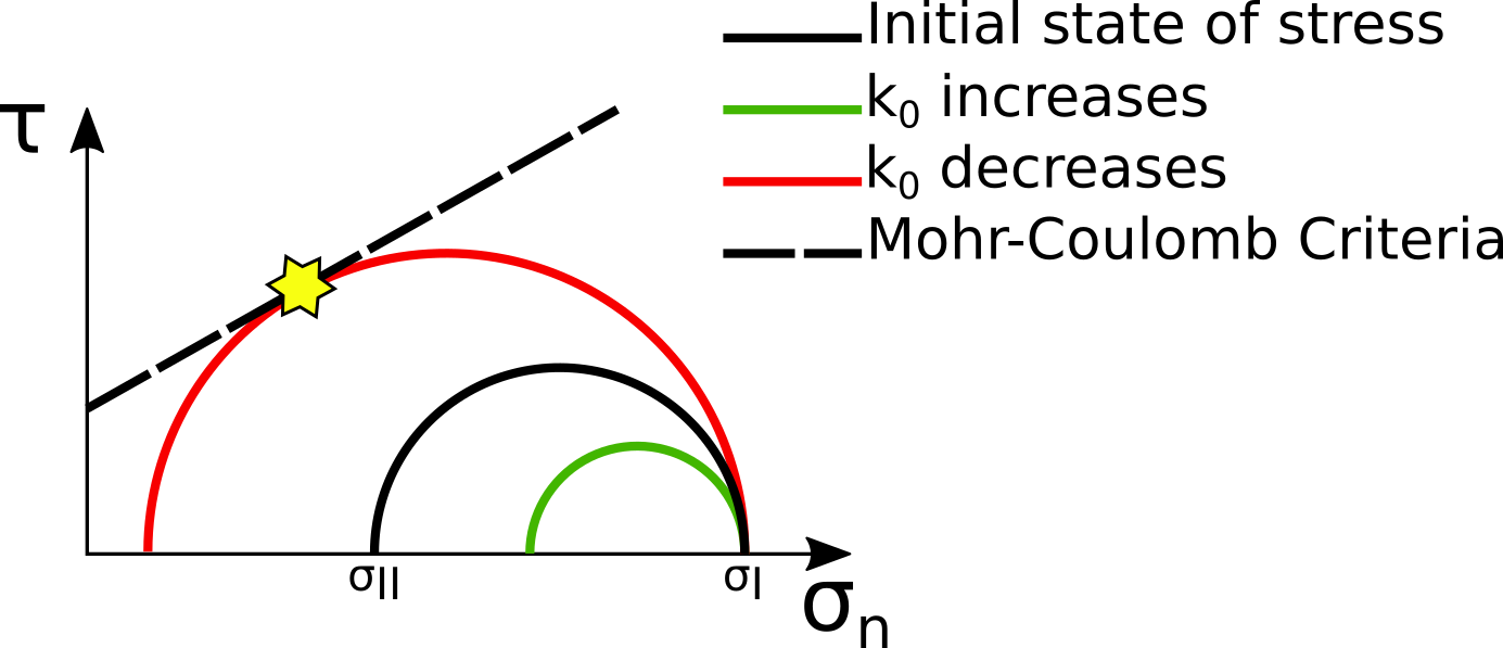
Figure 16: The effect of an increase or a decrease of the $k_{0}$ in the Mohr plane, a reduction of this parameter can induce a failure.

5.2 About the Young modulus reduction assumption

As formulated by Equation 24, the Young modulus and the mechanical properties are decreased with the weathering of the rock. This assumption has a huge influence on the evolution of the $k_{0}$, especially in the case $k_{0}^{init}\geq k_{0}^{attr}$, see Section 4.2. More than a numerical investigation to understand phenomena, the assumption has a deeper meaning. Indeed, the type of contacts and the load history of the sample can be modelled by this hypothesis.

As illustrated in Figure 17, the contact can be sorted into three types: I) Frictional, II) Mixed/Cohesive (Frictionnal+Cemented) or III) Cemented [18]. In case I there is no cement, so the Young modulus reduction assumption is not required. Otherwise, in the first approach, the contact can be modelled as two springs (one for the grains and one for the cement) in parallel (type II) or in series (type III). In those two cases (parallel or series), the Young modulus reduction assumption should be used depending on the history of loading, as discussed in the following paragraph. The difference between the two cases is based on the final value (after the entire dissolution of the bond) of the Young modulus $E_{m}^{final}$. In case II, it will be the value assumed for frictional contact (type I) $E_{m}^{I}$. In case III, it will be null (except if a new contact type I occurs).

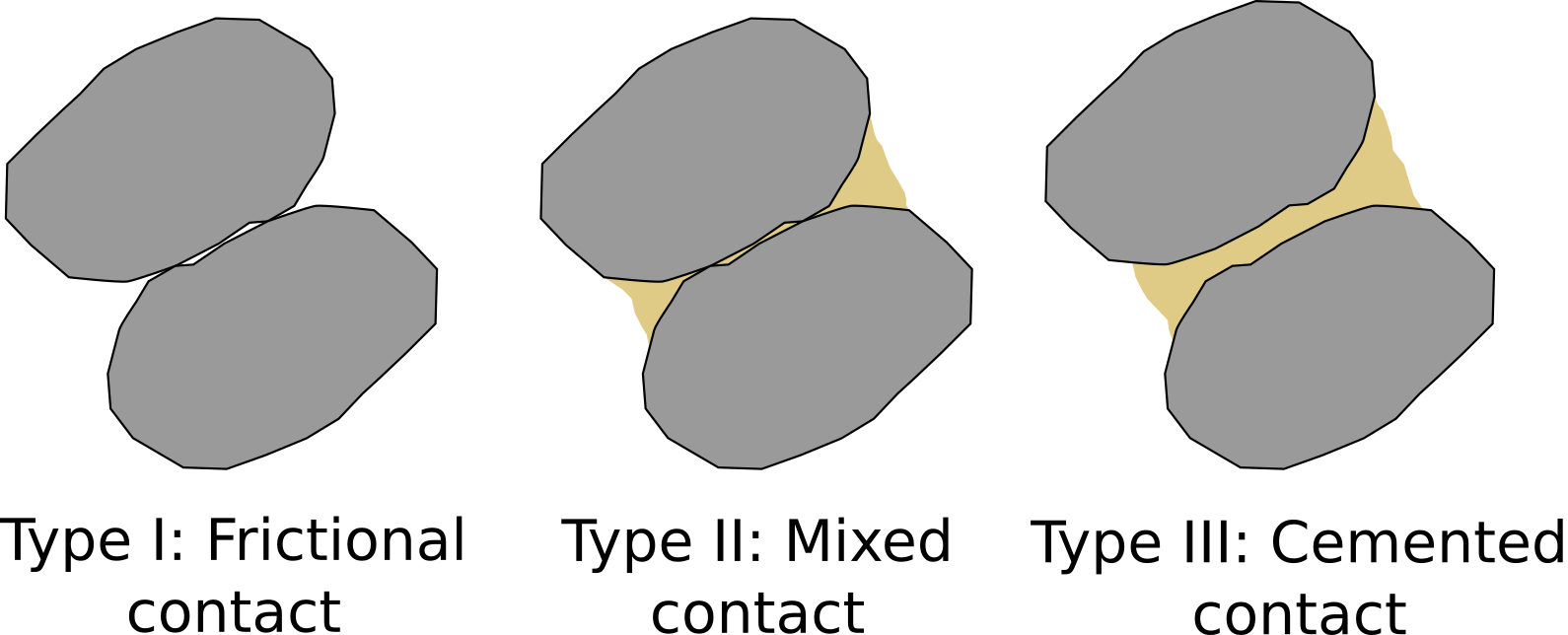
Figure 17: Definition of the contact types: I) Frictional, II) Mixed or cohesive (Frictionnal+Cemented) and III) Cemented.

As explained earlier in this Section, the Young modulus reduction assumption is applied for contacts type II and III, depending on the history of loading. As illustrated in Figure 18 and coming back to the initial model with springs in parallel or in series, the cementation that occurs at pressure $P_{i}$ is considered loaded only if the current pressure applied $P_{j}$ verifies $P_{j}>P_{i}$. The Young modulus reduction hypothesis should be applied only if the bonds are assumed loaded. This discussion is summarized in Table 3. In this work, loaded contacts type II have been used. Nevertheless, some results have been obtained for non-loaded contacts type II in Figure 8.

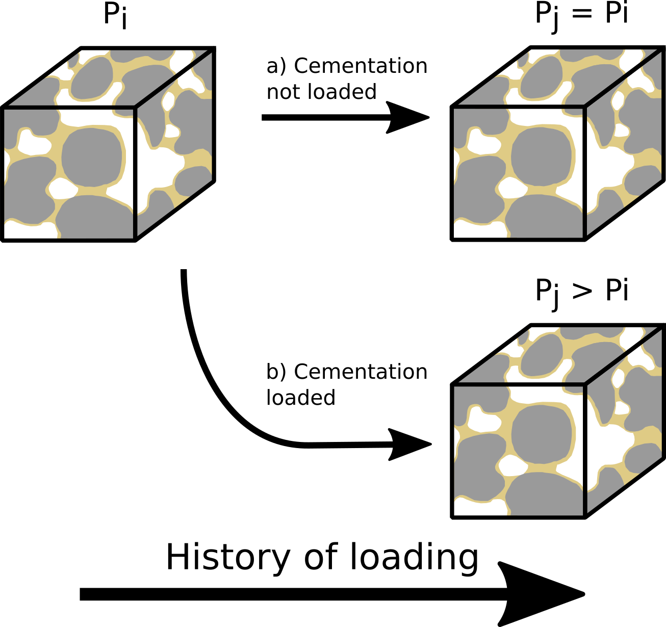
Figure 18: Depending on the history of loading, the cementation can be loaded or not. This scheme illustrates the fact that a cementation that occurred at $P_{i}$ can be considered a) not loaded if $P_{j}=P_{i}$ or b) loaded if $P_{j}>P_{i}$, where $P_{j}$ is the current pressure applied.

	Contact I	Contact II	Contact III
Bonds loaded	NO	YES ($E_{m}^{final}=E_{m}^{I})$	YES ($E_{m}^{final}=0)$
Bonds not loaded	NO	NO	NO

Table 3: Summarize the use of the Young modulus reduction assumption. If the hypothesis is applied, the final value of $E_{m}$ is given.

6 Conclusion

The debonding of the rock can be the origin of failure reactivation as mechanical properties weaken and the state of stress evolves. This influence of several parameters such as the degree of cementation, the confining pressure, the initial value of $k_{0}$ and the history of load are investigated in this paper.

It has been shown that an attractor configuration exists and the grain reorganization occurs during the debonding to reach this state. Especially, the $k_{0}$ evolves to its attractor value, increasing or decreasing. It appears that a $k_{0}$ reduction can be the origin of failure reactivation.

Two main mechanisms have been emphasized for the grain reorganization, depending on the initial state of stress. The chain forces need to be sorted into two kinds: the unstable and the stable chain forces. The unstable ones support the force thanks to the cementation, when the debonding occurs they collapse. On the opposite, the stable ones stay in place, even if they are no cementation. It appears that the unstable ones are dominant in the case $k_{0}^{init}\leq k_{0}^{attr}$ and the stable ones are dominant in the case $k_{0}^{init}\geq k_{0}^{attr}$. In the second case, the grain reorganization occurs with the grain softening.

7 Software

The Discrete Element Model is solved using the YADE open source software [38]. Some examples of scripts used are available on GitHub at the following link:

• https://github.com/AlexSacMorane/YADE_oedo_acid

8 Acknowledgements

This research has been partially funded by the Fonds Spécial de Recherche (FSR), Wallonia-Bruxelles Federation, Belgium. The work has also received funding from the National Science Foundation (NSF), USA, project CMMI-2042325.

Appendix A The lognormal distribution

The probability of a bond to have a surface $A_{b}$ follows a lognormal distribution formulated in Equation 31. This distribution is defined by the expected value $m_{log}$ and the variance $s_{log}$.

$$p(A_{b})=\frac{1}{A_{b}\,s_{log}\sqrt{2\pi}}e^{-\frac{\left(ln\left(A_{b}\right)-m_{log}\right)^{2}}{2\,s_{log}^{2}}}$$ (31)

It appears this distribution reproduces accurently experimental observations [18]. Indeed, smaller bond surfaces and larger ones can be considered, both are important to the mechanical behavior of the sample. Examples of lognormal distribution used in this paper are given in Figure 19.

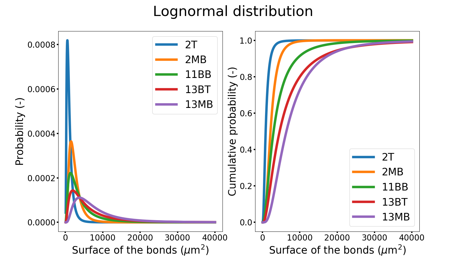
Figure 19: Examples of lognormal distributions used in this paper with the different cementations considered (see Table 2).

References

- [1] N. Heinemann, J. Alcalde, J. M. Miocic, S. J. Hangx, J. Kallmeyer, C. Ostertag-Henning, A. Hassanpouryouzband, E. M. Thaysen, G. J. Strobel, C. Schmidt-Hattenberger, K. Edlmann, M. Wilkinson, M. Bentham, R. Stuart Haszeldine, R. Carbonell, and A. Rudloff, “Enabling large-scale hydrogen storage in porous media-the scientific challenges,” Energy & Environ. Sci., vol. 14, pp. 853–864, 2023.
- [2] J. McCartney, M. Sanchez, and I. Tomac, “Energy geotechnics: Advances in subsurface energy recovery, storage, exchange, and waste management,” Comput. and Geotech., vol. 75, pp. 244–256, 2016.
- [3] M. Lesueur, T. Poulet, and M. Veveakis, “Three-scale multiphysics finite element framework (fe3) modeling fault reactivation,” Comput. Methods in Appl. Mech. and Eng., vol. 365, p. 112988, 2020.
- [4] K. Ramesh Kumar, H. Honorio, D. Chandra, M. Lesueur, and H. Hajibeygi, “Comprehensive review of geomechanics of underground hydrogen storage in depleted reservoirs and salt caverns,” J. of Energy Storage, vol. 73, p. 108912, 2023.
- [5] R. H. Brzesowsky, C. J. Spiers, J. Peach, and S. J. T. Hangx, “Time-independent compaction behavior of quartz sands,” J. Geophys. Res. Solid Earth, vol. 119, pp. 936–956, 2014.
- [6] A. Sac-Morane, M. Veveakis, and H. Rattez, “A Phase-Field Discrete514 Element Method to study chemo-mechanical coupling in granular materials,” Comput. Methods in Appl. Mech. and Eng., vol. 424, p. 116900,516 2024.
- [7] J. Rohmer, A. Pluymakers, and F. Renard, “Mechano-chemical inter-518 actions in sedimentary rocks in the context of storage: Weak acid, weak effects?,” Earth-Sci. Rev., vol. 157, pp. 86–110, 2016.
- [8] J. C. Manceau and J. Rohmer, “Post-injection trapping of mobile in deep aquifers: Assessing the importance of model and parameter uncertainties,” Comput. and Geosci., vol. 20, pp. 1251–1267, 2016.
- [9] H. Rattez, F. Disidoro, J. Sulem, and M. Veveakis, “Influence of dissolution on long-term frictional properties of carbonate fault gouge,” Geomech. for Energy and the Environ., vol. 26, p. 100234, 2021.
- [10] R. Castellanza and R. Nova, “Oedometric tests on artificially weathered527 carbonatic soft rocks,” J. of Geotech. and Geoenviron. Eng., vol. 130, pp. 728–739, 2004.
- [11] H. Shin and J. C. Santamarina, “Mineral dissolution and the evolution of ,” J. of Geotech. and Geoenviron. Eng., vol. 135, pp. 1141–1147, 2009.
- [12] V. Parol and A. Das, “Behavioural study on geomaterial undergoing chemo-mechanical degradation,” vol. 55, pp. 305–314, 2020.
- [13] M. Cha and J. C. Santamarina, “Dissolution of randomly distributed soluble grains: Post-dissolution k0-loading and shear,” Geotech., vol. 64, pp. 828–836, 2014.
- [14] M. Alam, V. Parol, and A. Das, “A dem study on microstructural behaviour of soluble granular materials subjected to chemo-mechanical loading,” Geomech. for Energy and the Environ., vol. 32, 2022.
- [15] H. Bayesteh and T. Ghasempour, “Role of the location and size of soluble particles in the mechanical behavior of collapsible granular soil: a dem simulation,” Comput. Part. Mech., vol. 6, pp. 327–341, 2019.
- [16] Z. Sun, D. N. Espinoza, and M. T. Balhoff, “Reservoir rock chemo-mechanical alteration quantified by triaxial tests and implications to fracture reactivation,” Int. J. of Rock Mech. and Min. Sci., vol. 106, pp. 250–258, 2018.
- [17] F. Bourrier, F. Kneib, B. Chareyre, and T. Fourcaud, “Discrete modeling of granular soils reinforcement by plant roots,” Ecol. Eng., vol. 61, pp. 646–657, 2013.
- [18] M. Sarkis, M. Abbas, A. Naillon, F. Emeriault, C. Geindreau, and A. Esnault-Filet, “D.E.M. modeling of biocemented sand: Influence of the cohesive contact surface area distribution and the percentage of cohesive contacts,” Comput. and Geotech., vol. 149, p. 104860, 2022.
- [19] A. Dadda, C. Geindreau, F. Emeriault, S. Rolland du Roscoat, A. Garandet, L. Sapin, and A. Esnault Filet, “Characterization of microstructural and physical properties changes in biocemented sand using 3d x-ray microtomography,” Acta Geotech., vol. 12, pp. 955–970, 2017.
- [20] E. Hoek, Practical Rock Engineering. RocScience, 2007.
- [21] M. H. Taherynia, S. M. Fatemi Aghda, and A. Fahimifar, “In-Situ Stress560 State and Tectonic Regime in Different Depths of Earth Crust,” Geotech. and Geol. Eng., vol. 34, pp. 679–687, 2016.
- [22] B. Demir, “K Ratios for Rock in Literature,” 2018. From https://www.linkedin.com/pulse/k-ratios-rock-literature-berk-demir.
- [23] P. A. Cundall, and O. D. Strack, “A discrete numerical model for granular assemblies,” Geotech., vol. 30, pp. 331–336, 1980.
- [24] C. O’Sullivan, Particulate Discrete Element Modelling. CRC Press, 2011.
- [25] J. Ai, J. F. Chen, J. M. Rotter, and J. Y. Ooi, “Assessment of rolling resistance models in discrete element simulations,” Powder Technol., vol. 206, pp. 269–282, 2011.
- [26] G. Mollon, A. Quacquarelli, E. Ando, and G. Viggiani, “Can friction replace roughness in the numerical simulation of granular materials ?,” Granul. Matter, vol. 22, p. 42, 2020.
- [27] A. Sac-Morane, M. Veveakis, and H. Rattez, “Frictional weakening of a575 granular sheared layer due to viscous rolling revealed by discrete element576 modeling,” Granul. Matter, vol. 26, 2024.
- [28] S. J. Burns and K. J. Hanley, “Establishing stable time-steps for dem simulations of non-collinear planar collisions with linear contact laws,” Int. J. for Numer. Methods in Eng., vol. 110, pp. 186–200, 2017.
- [29] G. Buscarnera and I. Einav, “The mechanics of brittle granular materials with coevolving grain size and shape,” Proc. R. Soc. A, vol. 477, p. 20201005, 2021.
- [30] P. Vaughan and C. Kwan, “Weathering, structure and in situ stress in residual soils,” Geotech., vol. 34, pp. 43–59, 1984.
- [31] F. Radjai, D. E. Wolf, M. Jean, and J.-J. Moreau, “Bimodal Character of Stress Transmission in Granular Packings,” Phys. Rev. Lett., vol. 80, pp. 61–64, 1998.
- [32] J. Shi and P. Guo, “Fabric evolution of granular materials along imposed stress paths,” Acta Geotech., vol. 13, pp. 1341–1354, 2018.
- [33] J. Liu, W. Zhou, G. Ma, S. Yang, and X. Chang, “Strong contacts, connectivity and fabric anisotropy in granular materials: A 3D perspective,” Powder Technol., vol. 366, pp. 747–760, 2020.
- [34] N. Guo and J. Zhao, “The signature of shear-induced anisotropy in granular media,” Comput. and Geotech., vol. 47, pp. 1–15, 2013.
- [35] J. Gong, J. Zou, L. Zhao, L. Li, and Z. Nie, “New insights into the effect of interparticle friction on the critical state friction angle of granular materials,” Comput. and Geotech., vol. 113, p. 103105, 2019.
- [36] A. J. Liu and S. R. Nagel, “Jamming is not just cool any more,” Nat., vol. 396, pp. 21–22, 1998.
- [37] J. Bares, M. Cardenas-Barrantes, D. Cantor, M. Renouf, and E. Azema, “Softer than soft: Diving into squishy granular matter,” Pap. in Phys., vol. 14, p. 140009, 2022.
- [38] V. Smilauer and al., Yade Documentation 3rd ed. The Yade Project, 2021.