Generalized Criterion for Identifiability of Additive Noise Models Using Majorization

Abstract

The discovery of causal relationships from observational data is very challenging. Many recent approaches rely on complexity or uncertainty concepts to impose constraints on probability distributions, aiming to identify specific classes of directed acyclic graph (DAG) models. In this paper, we introduce a novel identifiability criterion for DAGs that places constraints on the conditional variances of additive noise models. We demonstrate that this criterion extends and generalizes existing identifiability criteria in the literature that employ (conditional) variances as measures of uncertainty in (conditional) distributions. For linear Structural Equation Models, we present a new algorithm that leverages the concept of weak majorization applied to the diagonal elements of the Cholesky factor of the covariance matrix to learn a topological ordering of variables. Through extensive simulations and the analysis of bank connectivity data, we provide evidence of the effectiveness of our approach in successfully recovering DAGs. The code for reproducing the results in this paper is available in Supplementary Materials.

1 Introduction

One of the fundamental problems in science is learning causal relations from observational data. Directed acyclic graphical (DAG) models serve as valuable tools for representing conditional independence and causal relations among random variables. Nevertheless, learning DAGs solely from the observational data proves to be a difficult problem. This is primarily due to issues related to identifiability and the space of the potential DAGs growing super-exponential as the number of nodes increases.

A commonly used strategy for addressing the non-identifiability issue is to impose restrictions on the joint distribution. For instance, methods like PC (Spirtes et al., 2001), GES (Chickering, 2003) and other related methods (Zhang & Spirtes, 2015; Raskutti & Uhler, 2013) have demonstrated that, under certain assumptions such as faithfulness, it is possible to recover DAG up to the Markov equivalence class. However, it is timely to note that the majority of Markov equivalence classes contain more than one graph, making it difficult to uniquely determine the true underlying graph.

Recent research has addressed the challenge of recovering causal structures by introducing various constraints aimed at capturing the asymmetry between cause and effect. Shimizu et al. (2006) propose a method for identifying linear non-Gaussian additive noise models (ANM). Hoyer et al. (2008); Zhang & Hyvärinen (2009); Peters et al. (2011) establish conditions for the identifiability of nonlinear ANMs. Park & Raskutti (2018); Park & Park (2019) employ higher-order moments of the conditional distribution to demonstrate the identifiability of DAGs. The ideas behind these approaches can be succinctly summarized using the concept of complexity or uncertainty (Mooij et al., 2016; Glymour et al., 2019). In particular, it is generally anticipated that the complexity of a physical process that generates effect from cause should be lower in some way than the complexity of the backward process. In other words, the relationship between two variables in a model is asymmetrical rather than symmetrical (Simon, 1977). These ideas has been explored using Kolmogorov complexity in Janzing & Schölkopf (2010). Also see Peters et al. (2017). The aforementioned methods harness various complexity measures for both marginal and conditional probability distributions to achieve identifiability.

In a similar vein, several studies (Peters & Bühlmann, 2013; Loh & Bühlmann, 2014; Ghoshal & Honorio, 2018; Chen et al., 2019; Park, 2020) have employed (conditional) variance as a complexity measure to establish identifiability results. Notably, Peters & Bühlmann (2013) demonstrate the identifiability of linear Structural Equation Models (SEMs) with equal variances. Ghoshal & Honorio (2017, 2018); Chen et al. (2019) note that the arrangement of specific conditional variances implies the identifiability of DAGs. Furthermore, Park (2020) introduces more comprehensive criteria concerning conditional variances for nonlinear ANMs with unknown heterogeneous error variances.

In this paper, we establish the identifiability of ANMs by leveraging the concept of majorization (see Section 2 for definitions). We prove that our approach constitutes a generalization of previous identifiability results that employ conditional variance as a complexity measure (Peters & Bühlmann, 2013; Rajaratnam & Salzman, 2013; Loh & Bühlmann, 2014; Ghoshal & Honorio, 2017, 2018; Chen et al., 2019; Park, 2020). Additionally, we introduce a novel DAG structure learning algorithm called Majorized Cholesky diagonal (MaCho), which utilizes our established criterion to estimate a topological ordering of a DAG.

2 Preliminaries

A DAG $G=(V,E)$ consists of a set of nodes $V=\{1,2,\dots,p\}$ and a set of directed edges $E\subset V\times V$ with no directed cycles. For the quick introduction to Bayesian Networks and related terminology, see Appendix I and Koller & Friedman (2009). Throughout the paper we assume causal sufficiency, i.e. no hidden confounders and causal minimality.

ANMs are a special case of DAG models in which, for the mean zero random vector $\boldsymbol{X}\in R^{p}$, the joint distribution is defined by the following structural equation:

$$X_{j}=f_{j}(X_{\mbox{pa}{j}})+\varepsilon_{j},$$ (1)

where $\varepsilon_{j}$’s are independent for $j\in V$ with possibly different distribution with mean zero and hetereogenous variances and $\mbox{pa}_{j}$ denotes the parents of the variable $j$. A linear SEM is a special case of (1), in which $f_{j}$’s are linear. In vector formulation, linear SEM can be written as

$$\boldsymbol{X}=B\boldsymbol{X}+\boldsymbol{\varepsilon},$$ (2)

where $B\in R^{p\times p}$ is a weighted adjacency matrix such that $\beta_{ij}\neq 0$ indicates $X_{j}\rightarrow X_{i}$. From (2), the distribution of $\boldsymbol{X}$ is denoted by $\boldsymbol{X}\sim(\boldsymbol{0},\Sigma)$, where

$$\Sigma=(I-B)^{-1}\Lambda[(I-B)^{-1}]^{{}^{\prime}}.$$ (3)

and $\Lambda$ is a diagonal matrix that contains error variances.

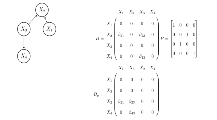
Figure 8: Illustration of DAG $\mathcal{G}$, corresponding coefficient matrix $B$, permutation matrix $P$, and permuted strictly lower triangular matrix $B_{\pi}$.

We say a DAG admits a topological ordering $\rho(\cdot)$, if $\rho(j)<\rho(k)$ then $k$ is not an ancestor of $j$, i.e. $k\not\in\mbox{An}(j)$, and a $p\times p$ permutation matrix $P_{\rho}$ can be associated such that $P_{\rho}\boldsymbol{x}=(x_{\rho(1)},\dots,x_{\rho(p)})$, for $\boldsymbol{x}\in R^{p}$. The existence of a topological ordering leads to the permutation-similarity of $B$ to a strictly lower triangular matrix $B_{\rho}=P_{\rho}BP^{{}^{\prime}}_{\rho}$ by permuting rows and columns of $B$, respectively (Bollen, 1989) (see Figure 8 in Appendix I for an illustrative example). Therefore,

$$\Sigma_{\rho}=(I-B_{\rho})^{-1}\Lambda_{\rho}[(I-B_{\rho})^{-1}]^{{}^{\prime}}=LL^{{}^{\prime}},$$ (4)

where $L=(I-B_{\rho})^{-1}\Lambda^{1/2}_{\rho}$ is a Cholesky factor of $\Sigma_{\rho}$.

The following Lemma will be useful in Section 5. The proof is provided in Appendix A for completeness. Also see Rajaratnam & Salzman (2013), for a similar result for autoregressive processes.

Lemma 2.1.

Suppose a random vector $\boldsymbol{X}$ generated from the linear SEM (2) with an ordering $\rho$, then for $1\leq j\leq p$

$$L^{2}_{j,j}=\mbox{var}(X_{\rho(j)}|X_{\rho(j-1)},\dots,X_{\rho(1)})$$ (5)

2.1 Majorization

The notion of majorization arises in a variety of branches of mathematics and statistics. Informally, majorization describes the notion that the components of a vector $\boldsymbol{x}\in R^{p}$ are less spread out or more nearly equal than the components of a vector $\boldsymbol{y}\in R^{p}$.

Formally, let $\boldsymbol{x}_{[\cdot]}$ denote the vector $x$ of a descending order, then we say $\boldsymbol{x}$ is majorized by $\boldsymbol{y}$, denoted $\boldsymbol{x}\prec\boldsymbol{y}$, if $\sum_{i=1}^{k}x_{[i]}\leq\sum_{i=1}^{k}y_{[i]}$, for $k=1,\dots,p-1$, and $\sum_{i=1}^{p}x_{[i]}=\sum_{i=1}^{p}y_{[i]}$. If $\sum_{i=1}^{p}x_{[i]}=\sum_{i=1}^{p}y_{[i]}$ does not hold, but $\sum_{i=1}^{p}x_{[i]}\leq\sum_{i=1}^{p}y_{[i]}$, then we say $\boldsymbol{y}$ weakly majorizes $\boldsymbol{x}$, i.e., $\boldsymbol{x}\prec_{w}\boldsymbol{y}$. (Weak) majorization defines a preordering on $R^{p}$.

Definition 2.2.

A linear transformation is called a $T$-transform, if

$$T=\lambda I+(1-\lambda)Q,$$

where $0\leq\lambda\leq 1$ and $Q$ is a permutation matrix that interchanges two coordinates.

That is $T\boldsymbol{x}=(x_{1},\dots,x_{j-1},\lambda x_{j}+(1-\lambda)x_{k},x_{j+1},\dots,\lambda x_{k}+(1-\lambda)x_{j},x_{k+1},\dots,x_{p})^{{}^{\prime}}$.

Theorem 2.3.

(Hardy et al. (1952)) For $\boldsymbol{x},\boldsymbol{y}\in R^{p}$, the following conditions are equivalent

1. $\boldsymbol{x}\prec_{w}\boldsymbol{y}$

2. $\boldsymbol{x}=P\boldsymbol{y}$ for some double substochastic matrix $P$

3. $\boldsymbol{x}$ can be derived from $\boldsymbol{y}$ by successive applications of a finite number of $T$-transformations, $\boldsymbol{x}\leq T_{1}\dots T_{k}\boldsymbol{y}$

The next theorem will be useful to proving identification results in Section 3.

Theorem 2.4.

(Marshall et al. (2011, Theorems 3.A.8a and 3.C.2.D)) Let $f$ be a real-valued function defined on the $A\in R^{p}$. Then

$$\boldsymbol{x}\prec_{w}\boldsymbol{y}\implies f(\boldsymbol{x})<f(\boldsymbol{y})$$

if and only if $f$ is strictly increasing, symmetric, and strictly convex in $A$.

3 Identifiability via Majorization

For the rest of the paper, we omit the subscript for a topological ordering of the graph $G$, denoted as $\rho_{0}$, whenever there is no potential for confusion. Without loss of generality, we assume $\rho_{0}=\{1,\dots,p\}$ and use $\rho$ to represent any other ordering. This notation simplification helps avoid the need for the longer notation ${\rho_{0}(1),\dots,\rho_{0}(p)}$.

As we discussed in Section 1, our focus is on identifiability conditions whereas a complexity measure, the (conditional) variance, has been employed. Recall that the concept of complexity or uncertainty implies that it is expected that the physical process that is generated using a topological ordering of variables should be ”simpler” than the process generated using other non-topological orderings. As a measure of the ”simplicity” of the process and to capture the asymmetry between cause and effect, we impose a weak majorization assumption. This means if the vector $\boldsymbol{x}$ contains the conditional variances using a topological ordering

$$\boldsymbol{x}=\{\mbox{var}(X_{1}),\dots,E[\mbox{var}(X_{p}|X_{1},\dots,X_{p-1})]\}^{{}^{\prime}}$$ (6)

and $\boldsymbol{y}_{\rho}$ contains conditional variances using any other ordering

$$\boldsymbol{y}_{\rho}=\{\mbox{var}(X_{\rho(1)}),\dots,E[\mbox{var}(X_{\rho(p)}|X_{\rho(1)},\dots,X_{\rho(p-1)})]\}^{{}^{\prime}},$$ (7)

then we anticipate $\boldsymbol{x}$ be less spread out then $\boldsymbol{y}_{\rho}$. Using language introduced in Section 2.1, $\boldsymbol{x}\prec_{w}\boldsymbol{y}_{\rho}$ for all permutations $\rho\in\mathfrak{S}_{p}$, where $\mathfrak{S}_{p}$ denotes the group of all permutations $\boldsymbol{X}$. Next, we state the main assumption of this paper.

Assumption 1.

Let $\boldsymbol{X}$ be generated from an ANM (1) with DAG $G$, then assume $\boldsymbol{x}\prec_{w}\boldsymbol{y}_{\rho}$ for all permutations $\rho\in\mathfrak{S}_{p}$, where $\boldsymbol{x}$ and $\boldsymbol{y}_{\rho}$ are defined in (6) and (7), respectively.

Remark 3.1.

The notion of varsortability, introduced by (Reisach et al., 2021), serves as a measure of agreement between the order of increasing marginal variance and the causal order. In Appendix H, we demonstrate that Assumption 1 holds even when the varsortability is low.

To provide an intuition how the Assumption 1 implies identification, we provide examples on bivariate ANMs generated from the following three DAGs:

(a) $G_{1}$

(b) $G_{2}$

(c) $G_{3}$

From Theorem 2.4, the following identification result holds:

$$\mbox{DAG}:=\begin{cases}G_{1},&\mbox{if }f(\boldsymbol{x})<f(\boldsymbol{y}_{\rho})\\ G_{2},&\mbox{if }f(\boldsymbol{x})>f(\boldsymbol{y}_{\rho})\\ G_{3},&\mbox{otherwise}\end{cases},$$ (8)

where $\boldsymbol{x}=[\mbox{var}(X_{1}),E[\mbox{var}(X_{2}|X_{1})]]^{{}^{\prime}}$, $\boldsymbol{y}_{\rho}=[\mbox{var}(X_{2}),E[\mbox{var}(X_{2}|X_{1})]]^{{}^{\prime}}$ and in this paper, we use Euclidean norm

$$f(\boldsymbol{x})=\|\boldsymbol{x}\|_{2}.$$ (9)

For other possible options for $f$, see Marshall et al. (2011). Empirical results, for bivariate case is provided in Section 6.

The next theorem generalizes the discussed bivariate case. Proof is provided in Appendix B.

Theorem 3.2.

If the Assumption 1 holds then DAG $G$ is uniquely identified.

4 Weak majorization as a generalized condition

In this section, we show that the weakly majorization Assumption 1 is a generalization of the existing identification conditions for nonlinear ANM (Park, 2020), linear SEM (Peters & Bühlmann, 2013; Loh & Bühlmann, 2014; Ghoshal & Honorio, 2018; Chen et al., 2019; Park, 2020) and autoregressive processes (Rajaratnam & Salzman, 2013).

For the nonlinear ANMs, defined in (1), Hoyer et al. (2008); Mooij et al. (2009); Peters et al. (2011) prove the identifiable classes of ANM by imposing restrictions on the functions $f_{j}$ or the joint distribution. Park (2020) used conditional independencies as an uncertainty measure to propose conditions listed in Assumption 2, for identification.

Assumption 2.

Let $\boldsymbol{X}$ be generated from an ANM (1), then assume for $k\in\mbox{De}(j)$ and $l\in\mbox{An}(j)$

1. $\sigma_{j}^{2}<\sigma_{k}^{2}+E(\mbox{var}(E(X_{k}|X_{\mbox{Pa}{k}})|X_{1},\dots,X_{j-1}))$

2. $\sigma_{j}^{2}>\sigma_{l}^{2}-E(\mbox{var}(E(X_{l}|X_{1},\dots X_{j-1}\char 92\relax X_{l})|X_{\mbox{Pa}{l}}))$

Moreover, Park (2020, Theorem 4) shows that Assumption 2 is a generalization of conditions proposed in Peters & Bühlmann (2013); Loh & Bühlmann (2014); Ghoshal & Honorio (2018); Chen et al. (2019). Consequently, our goal is to show that Assumption 2 implies the weakly majorization of conditional variances, given in Assumption 1.

Theorem 4.1.

If the conditions of Assumption 2 are satisfied, then Assumption 1 is also satisfied.

Proof is provided in Appendix C. It is imperative to consider cases where Assumption 2 is violated but Assumption 1 holds. In Appendix D, we show that Assumption 2 is a special case of our Assumption 1. That is there are cases when Assumption 2 is violated but Assumption 1 holds.

5 Algorithm

The proof of Theorem 3.2 provides a recipe for learning topological ordering of a DAG. In particular, we can exploit Theorem 2.4 to compare the estimated value of (9) for all permutation $\rho\in\mathfrak{S}_{p}$ and choosing the one that obtains a minimum value

$$\min_{\rho}f(y_{\rho}).$$

Unfortunately, for large $p$ this strategy is computationally infeasible, since $\mathfrak{S}_{p}$ is large and it requires comparing values of $p!$ permutations.

In this section, we propose an algorithm, named Majorized Cholesky Diagonal (MaCho), that learns the topological ordering of the DAG generated from the linear SEM (2) with $O(p^{3})$ computational cost.

The intuition behind the proposed algorithm can be explained best by assuming that the index of the first variable is known, and then considering how the algorithm will learn the rest of the ordering on the Cholesky factor of the population covariance matrix. The MaCho algorithm proceeds recursively as follows. Given an already recovered ordering of the unknown permutation $\rho$, denoted $\rho_{m}=\{{\rho(1)},{\rho(2)},\dots,{\rho(m)}\}$ of size $m<p$, the algorithm chooses the next index $i_{\rho(m+1)}$ to minimize the $\ell_{2}$ norm of the diagonal of Cholesky factor

$$f( \mbox{dichol}[\Sigma_{\rho_{m}\cup\rho(m+1),\rho_{m}\cup\rho(m+1)}])=$$ (10)

$$\sqrt{L^{2}_{{\rho(1)},{\rho(1)}}+L^{2}_{{\rho(2)},{\rho(2)}}+\dots+L^{2}_{{\rho(m+1)},{\rho(m+1)}}},$$

where $\mbox{dichol}(A)=\mbox{diag}(\mbox{Cholesky}[A])$ denotes an operator that extracts the diagonal values of the Cholesky factor and $\Sigma_{\rho_{m},\rho_{m}}$ denote the submatrix of $\Sigma$ with corresponding indices $\rho_{m}=\{{\rho(1)},{\rho(2)},\dots,{\rho(m)}\}$. Lemma 2.1 and (9) provide a mathematical justification for (10). When the index of the first variable is unknown, in each iteration we check if

$$f(\mbox{dichol}[\Sigma_{\rho_{m}\cup{\rho(m+1)},\rho_{m}\cup{\rho(m+1)}}])\leq$$ (11)

$$f(\mbox{dichol}[\Sigma_{{\rho(m+1)}\cup\rho_{m},{\rho(m+1)}\cup\rho_{m}}])$$

then we add $\rho(m+1)$ at the end of $\rho_{m}$, otherwise in front of $\rho_{m}$ and ${\rho(m+1)}$ becomes the first index. Algorithm 1 summarizes the steps.

Algorithm 1 MaCho

  Input: $p\times p$ sample or sparse covariance matrix $S$

  Select any index as $\rho(1)$.

  Set $\rho_{1}=\{\rho(1)\}$

  for $i=2$ to $p$ do

     Choose the next index

$$\rho(i)=\min_{i,\dots,p}f(\mbox{dichol}[S_{\rho_{i-1}\cup{\rho(i)},\rho_{i-1}\cup{\rho(i)}}])$$

     if (11) is TRUE then

        $\rho_{i}=\{\rho_{i-1},\rho(i)\}$

     else

        $\rho_{i}=\{\rho(i),\rho_{i-1}\}$

     end if

  end for

  Output: $\rho_{p}$

In practice, when the number of observations is greater than the dimension of variables, i.e. $n>p$, we suggest to recover the variable ordering using a modified version of the Cholesky factor of the sample covariance matrix $S=\hat{L}\hat{L}^{{}^{\prime}}$, which is asymptotically unbiased estimator of the population Cholesky factor. The modified version, is defined as $\tilde{L}=\hat{L}\Omega$, where

$$\Omega=\mbox{diag}(1/n,\dots,1/n-j+1,\dots,1/n-p+1).$$

The proof of the next lemma is relegated to Appendix F.

Lemma 5.1.

Let $\boldsymbol{X}\sim N_{p}(0,\Sigma)$. As $n\rightarrow\infty$, $E(\tilde{L})=L$ with probability tending to 1.

For high dimensional dataset, when $n<p$, the covariance matrix can be estimated using a well known sparse covariance matrix estimation methods such as Bien & Tibshirani (2011); Wang (2014). Throughout the paper, when $n<p$, we adopt covariance graphical lasso algorithm proposed in Wang (2014) and implemented in R package covglasso available via CRAN.

5.1 Computational details

One of the main computational cost in Algorithm 1 is in the computation of $\min_{i,\dots,p}f(\mbox{dichol}[S_{\rho_{i-1}\cup{\rho(i)},\rho_{i-1}\cup{\rho(i)}}])$ in each iteration $i$. Fortunately, there is no need to implement Cholesky factorization on the $i\times i$ matrix in each iteration $i$. The new Cholesky factor can be found utilizing the estimated $(i-1)\times(i-1)$ Cholesky factor $L^{(i-1)}$ from iteration $i-1$. In particular, the new added row of $L^{(i)}$ can be computed (Golub & Van Loan, 1996), for $j=1$

$$L^{(i)}_{i,j}=\frac{S_{i,j}}{L^{(i-1)}_{j,j}},$$

for $j=2,\dots,i-1$

$$L^{(i)}_{i,j}=\frac{1}{L^{(i-1)}}(S_{i,j}-\sum_{k=1}^{j-1}L^{(i)}_{i,k}*L^{(i-1)}_{j,k})$$

and for $j=i$

$$L_{i,i}=\sqrt{S_{i,i}-\sum_{k=1}^{i-1}(L^{(i)})^{2}_{i,k}}$$

This requires $O(i^{2})$ flops in each iteration $i$. The next computational burden is in computing (11). Again this can be computed in $O(i^{2})$ flops, using the Cholesky factorization update algorithm in Davis & Hager (2005) and Golub & Van Loan (1996, Chapter 12.5). From the above discussion, the following lemma easily follows.

Lemma 5.2.

The Algorithm 1 has a computational cost $O(p^{3})$.

5.2 Estimation algorithm

Algorithm 1 provides a procedure to estimate a topological ordering of the DAG. Given the ordering, there exist a rich literature on estimating the DAG structure, such as Shojaie & Michailidis (2010); Khare et al. (2019); Park (2020). Motivated by the encouraging results of thresholding estimators for the (inverse) covariance matrix (Cai et al., 2016; Wang & Allen, 2022), we propose to use the thresholded version of Convex Sparse Cholesky Selection (CSCS) algorithm introduced in Khare et al. (2019). CSCS minimizes the following objective function

$$\mbox{tr}(LL^{{}^{\prime}}S)-2\log|L|+\lambda\sum_{1\leq j<i\leq p}|L_{ij}|$$ (12)

Then our final estimator is

$$\hat{L}^{\tau}=\hat{L}1(|\hat{L}|>\tau),$$ (13)

where $1(\cdot)$ is the indicator function, and $\hat{L}$ is a CSCS estimator. The next theorem shows the sign consistency of thresholded CSCS under the following conditions:

• A1 Marginal sub-Gaussian assumption: The sample matrix $X\in\mathcal{R}^{n\times p}$ has $n$ independent rows with each row drawn from the distribution of a zero-mean random vector $X=(X_{1},\dots,X_{p})^{t}$ with covariance $\Sigma$ and sub-Gaussian marginals; i.e.,

  $$E[\mbox{exp}(tX_{j}/\sqrt{\Sigma_{jj}})]\leq\mbox{exp}(Ct^{2})$$

  for all $j=1,\dots,p,\,t\leq 0$ and for some constant $C>0$.

• A2 Sparsity Assumption: The true Cholesky factor $L\in\mathcal{R}^{p\times p}$ is the lower triangular matrix with positive diagonal elements and support $\mathcal{S}(L)=\{(i,j),i\neq j|L_{ij}\neq 0\}$. We denote by $s=|S|$ cardinality of the set $S$.

• A3 Bounded eigenvalues: There exist a constant $\kappa$ such that

  $$0<\kappa^{-1}\leq\lambda_{min}(L)\leq\lambda_{max}(L)\leq\kappa$$

• A4 The minimum edge strength:

  $$\ell_{\min}:=\min_{1\leq j<i\leq p}|L_{ij}|>c_{1}\sqrt{\frac{s\log p}{n}}$$ (14)

Theorem 5.3.

Let the Assumptions 1-3 be satisfied. Further, if Assumption 4 is satisfied with $c_{1}>2c_{2}$, where $c_{2}$ is defined in Lemma G.1, the thresholded CSCS estimate $\hat{L}^{\tau}$ with threshold level $\tau=c_{2}\sqrt{\frac{s\log p}{n}}$ satisfies:

$$\mbox{sign}(\hat{L}^{\tau})=\mbox{sign}(L_{ij}),\;\forall{i\neq j}$$ (15)

with probability tending to 1.

The proof is provided in Appendix G. Theorem 5.3 provides an additional support to our usage of thresholded CSCS, since the estimated model with reversed signs can be misleading and hardly qualifies as a correctly selected model (Zhao & Yu, 2006).

6 Numerical results

In this section, we measure the performance of the proposed criterion and the algorithm using various simulation results.

6.1 Bivariate non-linear ANM

We start our analysis by considering the bivariate case, as discussed in (8), while incorporating heterogeneous error variances using both Gaussian and non-Gaussian distributions. Similar to Park (2020), as a non-linear ANM, we select a polynomial SEM where each variable is modeled as a 5th-degree polynomial in relation to its parents. In the Gaussian scenario, error variances are randomly chosen from the range $\sigma_{j}^{2}\in[0.7,1.2]$, while in the non-Gaussian case, we employ Gaussian mixture models. For each of these cases, we generate 100 sets of samples, each with the number of observations set at $n=500$.

We then proceed to compare our results with the method proposed in Hoyer et al. (2008), referred to as NCD, and utilize the Causal Discovery package in Python (Kalainathan & Goudet, 2019). In our method, the non-linear ANM is estimated using Random Forest (Breiman, 2001). We generate causal effect relationships, such as $x\rightarrow y$, $x\leftarrow y$, and no effect, with probabilities of $\{0.4,0.4,0.2\}$, respectively. From (8), given that achieving exact equality for the ”no-effect” scenario is challenging, we introduce a tolerance measure denoted as $\mu$, defined as:

$$\mu=\frac{|f(x)-f(y)|}{\max(f(x),f(y))},$$

This measure quantifies the allowed relative difference in magnitude that still qualifies as the absence of a causal effect. Based on the simulation results, we recommend $\mu=0.1$. A similar measure is also defined for the NCD method for the sake of comparison.

Table 1 reports the accuracy of both methods, where accuracy indicates the correct identification of the direction of the causal effect or the identification of a ”no-effect” scenario. As evident from the table, our method outperforms NCD for both Gaussian and non-Gaussian cases.

Table 1: Estimated accuracy for the bivariate case

Method	Gaussian	Non-Gaussian
Our	0.95	0.93
NCD	0.91	0.90

6.2 Multivariate linear SEM

For the multivariate linear modeling, we explore three distinct scenarios: 1) Gaussian homogeneity, 2) Gaussian heterogeneity, and 3) non-Gaussian heterogeneity. In all three scenarios, we generate data based on the Structural Equation Model (SEM) described in Equation (2).

In the case of Gaussian homogeneity, we set all noise variances equal to $\sigma^{2}=0.7$. For the Gaussian heterogeneity scenario, error variances are randomly selected from the range $\sigma_{j}^{2}\in[0.7,1.7]$. Finally, in Case 3, data is generated from a mixed Gaussian distribution.

(a) Case 1

(b) Case 2

(c) Case 3

Figure 2: Comparison of the proposed algorithm MaCho, BU, TD, and LINGAM algorithms in terms of average TPR, TDR, and SHD for recovering linear SEM with different error variances and $p=20$.

We proceed to compare the performance of our proposed MaCho algorithm with that of the bottom-up (BU) method (Ghoshal & Honorio, 2017), the top-down (TD) method (Chen et al., 2019), and the LINGAM algorithm (Shimizu et al., 2006). For BU and TD algorithms, we employ the R package EqVarDAG, and for LINGAM, we utilize pcalg. Both packages are available via CRAN. For BU and TD, we select the hyperparameter $\lambda$ through a 10-fold cross-validation and for MaCho we use procedure described in Wang & Allen (2022, Section 3.4).

We evaluate the performance of our algorithm and the comparative methods by varying the sample size $n$ across the set $\{250,500,1000,1500\}$ and the dimensionality $p\in\{20,50,100\}$. The performance assessment is based on metrics such as the true positive rate (TPR), true discovery rate (TDR), and Structural Hamming Distance (SHD), and we conduct this evaluation over 100 replications.

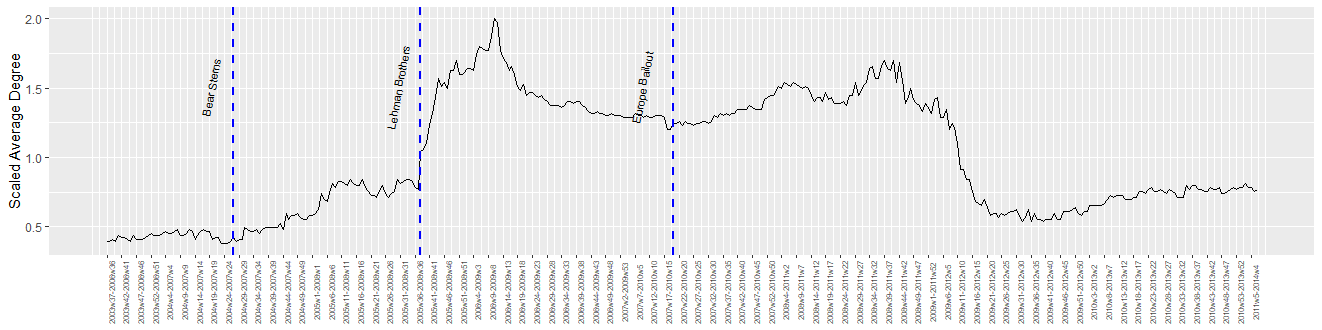
Figure 3: Evolution of average degree of bank connectedness scaled by their historic average (over 2003-2014).

Figure 2 presents the results, and it’s evident that LINGAM performs the least effectively in both Case 1 and Case 2. In Case 3, LINGAM shows behavior similar to the other algorithms when the sample size n exceeds 1000. Overall, the performance of MaCho, BU, and TD are quite comparable. For a more detailed illustration of their performance (excluding LINGAM), please refer to Figure 11 in the Appendix. The figure reveals that in Case 2, the performance of MaCho slightly outperforms BU and TD across all three evaluation metrics.

In Figure 4, we present results for $p=200$ without the LINGAM algorithm. It is evident that MaCho achieves the highest TPR in all three cases. In terms of the other metrics, the performance of MaCho and TD is very close for all cases. Appendix J.2 contains results for $p=50$.

6.3 Case study: Bank Network Connectedness

We employ the MaCho algorithm to detect the global bank network connectedness. The original dataset (Demirer et al., 2018) comprises 96 banks from 29 developed and emerging economies (countries), spanning the period from September 12, 2003, to February 7, 2014. To enhance clarity, we narrow our focus to economies with more than four banks, resulting in a selection of 54 banks (for further details, please refer to Demirer et al. (2018)). To analyze the data, we adopt a commonly used rolling window procedure (Xue et al., 2012; Basu et al., 2023) estimating the model using a 3-year rolling window.

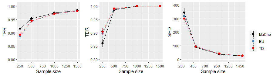
(a) Case 1

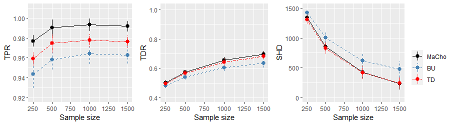
(b) Case 2

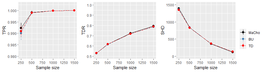
(c) Case 3

Figure 4: Comparison of the proposed algorithm MaCho, BU, TD, and LINGAM algorithms in terms of average TPR, TDR, and SHD for recovering linear SEM with different error variances and $p=200$.

Our investigation into bank connectedness involves studying the evolution of bank networks through the average number of direct neighbors. Figure 3 depicts the average degree of the network over 3-year rolling windows. The plot clearly demonstrates that the connectedness, as measured by the count of neighbors, increases both before and during significant systematic events. Notably, we observe several prominent cycles in Figure 3, with three key events marked, the first two corresponding to the failures of Bear Stearns and Lehman Brothers, which marked the financial crisis of 2007-2009. The final event corresponds to the European Bailout. Our findings align with existing results in the literature, including those in Basu et al. (2023, Section 4) and Billio et al. (2012). For comparative analysis, please refer to Appendix J.1, where we present results for LINGAM.

In Figure 5, we present DAGs corresponding to bank connectedness both before and after the Lehman Brothers’ failure. In this figure, the colors of the nodes represent the respective countries to which the banks belong. As anticipated, the DAG estimated after the Lehman Brothers’ failure exhibits a notably denser structure.

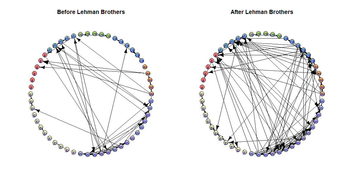
Figure 5: The DAG estimated from MaCho network for the pre and post Lehman Brothers failure.

Another intriguing question pertains to how bank connectedness evolved within individual countries. To address this, we treat each country as a distinct component and estimate both intra- and inter-connectedness. In Figure 6, the red dotted line represents the average degrees within banks in the USA and Italy. The black solid and blue dashed lines correspond to the estimated average degrees of in-edges and out-edges of the country as a component. In this context, in-edges signify changes within the country’s causal relationships, while out-edges signify how banks in the country influence banks in other countries.

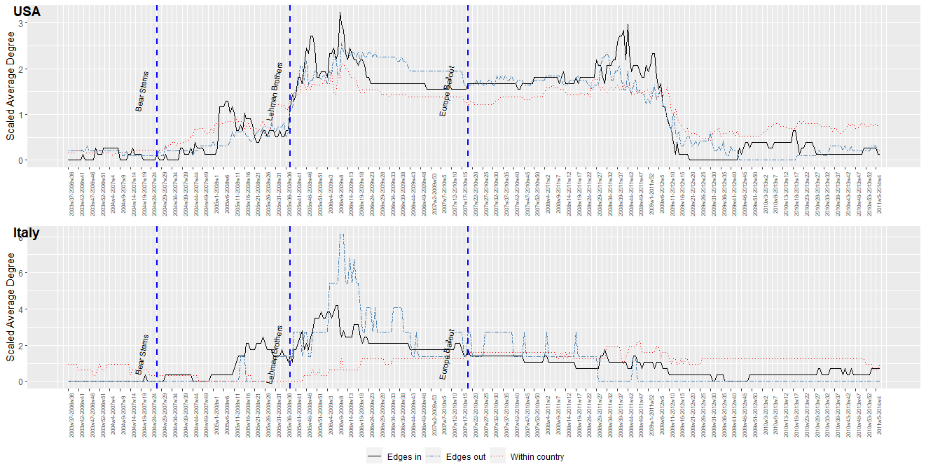
Figure 6: Evolution of average intra and inter-degree of bank connectedness scaled by their historic average (over 2003- 2014). (Top) USA and (Bottom) Italy.

A visible contrast emerges in the evolution of network connectedness between these two countries. In the USA, all three lines exhibit similar behavior, indicating that connectedness tends to grow before and during significant events. However, in Italy, the growth of within connectedness occurs much more gradually when compared to the average degree of out-edges.

7 Conclusion and Discussion

In this paper, we have introduced a novel identifiability condition for ANMs with heterogeneous error variances. Our work demonstrates that ANMs can achieve identifiability without the need to assume linearity and Gaussianity. For linear SEMs, we have presented the MaCho algorithm, which is designed for learning the topological ordering of DAGs. Our findings are supported by various numerical experiments, which empirically confirm that MaCho successfully learns the true topological ordering.

One prominent area for future research involves exploring the testing of the weakly majorization condition for ANMs when the dimensionality $p$ is large. We have demonstrated that empirical testing of the weakly majorization assumption is feasible for smaller dimensions, but the computational costs become prohibitively high as $p$ increases.

Appendix A Proof of Lemma 2.1

In this section, we show that the diagonal elements of the Cholesky factor of the covariance matrix $\Sigma_{\rho}$ have a probabilistic interpretation as the conditional variances.

From (2), $\boldsymbol{\varepsilon}=(I-B_{\rho})^{-1}\boldsymbol{X}$. That is for $2\leq j\leq p$,

$$\varepsilon_{\rho(j)}=X_{\rho(j)}+\sum_{i=1}^{j-1}U_{\rho(j),\rho_{o}(i)}X_{\rho(i)},$$

where $U_{\rho_{0}}=(I-B_{\rho})^{-1}$. Since by definition of SEM, for $\rho(k)<\rho(j)$, $\varepsilon_{\rho(j)}\perp\!\!\!\perp X_{\rho(k)}$ then

$$\mbox{var}(\varepsilon_{\rho(j)}) =\mbox{var}(\varepsilon_{\rho(j)}|X_{\rho(1)},\dots,{\rho(j-1)})=\mbox{var}(X_{\rho(j)}+\sum_{i=1}^{j-1}U_{\rho(j),\rho(i)}X_{\rho(i)}|X_{\rho(1)},\dots,X_{\rho(j-1)})$$

$$=\mbox{var}(X_{\rho(j)}|X_{\rho(1)},\dots,X_{\rho(j-1)})$$

Since $\Sigma_{\rho}=LL^{{}^{\prime}}$ is the unique Cholesky decomposition, from (4), the result follows.

Appendix B Proof of Theorem 3.2

The first part of the proof adapts a similar idea and technique as Theorem 1 in Peters & Bühlmann (2013). We assume that there are two models as in (1) with DAGs $G$ and $G^{{}^{\prime}}$ respectively, such that both induce the same joint distribution. We will show by contradiction that $G=G^{{}^{\prime}}$. By definition, DAGs contain nodes that have no child, such that eliminating such nodes from the graph leads to a DAG again. Consequently, in both $G$ and $G^{{}^{\prime}}$, we remove all nodes that have no children but have the same parents in both graphs. If there are no remaining nodes, the two graphs are identical and the result follows. Otherwise, we obtain two smaller DAGs, which we again call $G$ and $G^{{}^{\prime}}$. It is important to note that, there exists at least one node $L$ in $G$ that has no children and is such that either the parents sets $\mbox{Pa}^{G}_{L}\neq\mbox{Pa}_{L}^{G^{{}^{\prime}}}$ or $\mbox{Ch}_{L}^{G^{{}^{\prime}}}\neq\emptyset$. Therefore, from Markov property of the distribution with respect to $G$, all other nodes of the graph are independent from $L$ given its parents

$$L\perp\!\!\!\perp\boldsymbol{X}\char 92\relax(\mbox{Pa}_{L}^{G}\cup L)|\mbox{Pa}_{L}^{G}$$

For the rest of the proof, it is informative to partition the parents of $L$ in $G$ into $\boldsymbol{Y},\boldsymbol{Z}$ and $\boldsymbol{W}$ (for illustration, see Figure 7), where $\boldsymbol{Z}$ are also parents of $L$ in $G^{{}^{\prime}}$, the $\boldsymbol{Y}$ are children of $L$ in $G^{{}^{\prime}}$, and the $\boldsymbol{W}$ are not adjacent to $L$ in $G^{{}^{\prime}}$. Let $\boldsymbol{D}$ be the $G^{{}^{\prime}}$ parents of $L$ that are not adjacent to $L$ in $G$ and $\boldsymbol{E}$ be the $G^{{}^{\prime}}$ children of $L$ that are not adjacent to $L$ in $G$. Thus we have $\mbox{Pa}_{L}^{G}=\boldsymbol{Y}\cup\boldsymbol{Z}\cup\boldsymbol{W}$ , $\mbox{Ch}_{L}^{G}=\emptyset$, $\mbox{Pa}_{L}^{G^{{}^{\prime}}}=\boldsymbol{Z}\cup\boldsymbol{D}$ and $\mbox{Ch}_{L}^{G^{{}^{\prime}}}=\boldsymbol{Y}\cup\boldsymbol{E}$.

(a) Part of $G$

(b) Part of $G^{{}^{\prime}}$

Figure 7: Partition of the nodes in $G$ and $G^{{}^{\prime}}$.

From Peters et al. (2014, Proposition 29), there exist a node $Y\in\boldsymbol{Y}$, such that for the sets $\boldsymbol{Q}:=\mbox{Pa}_{L}^{G}\char 92\relax\{Y\},\,\boldsymbol{R}:=\mbox{Pa}_{Y}^{G^{{}^{\prime}}}\char 92\relax\{L\}$ and $\boldsymbol{S}:=\boldsymbol{Q}\cup\boldsymbol{R}$ we have $\boldsymbol{S}\subset\mbox{Nd}_{L}^{G}\char 92\relax\{Y\}$ and $\boldsymbol{S}\subset\mbox{Nd}_{Y}^{G^{{}^{\prime}}}\char 92\relax\{L\}$. Take any $\boldsymbol{s}=(\boldsymbol{q,r})$ and denote $L^{*}:=L|_{\boldsymbol{S=s}}$ and $Y^{*}:=Y|_{\boldsymbol{S=s}}$. From $G$, we can write

$$L^{*}=f_{L}(\boldsymbol{q},Y^{*})+\varepsilon_{L}$$

such that $\varepsilon_{L}\perp\!\!\!\perp Y^{*}$, since $\boldsymbol{S}\subset\mbox{Nd}_{L}^{G}\char 92\relax\{Y\}$. Applying the majorization Assumption 1 and denoting $\boldsymbol{x}=[\mbox{var}(Y^{*}),E[\mbox{var}(L^{*}|Y^{*})]]^{{}^{\prime}}$, from Theorem 2.4, $f(\boldsymbol{x})<f(\tilde{\boldsymbol{x}})$, where $\tilde{\boldsymbol{x}}=[\mbox{var}(L^{*}),E[\mbox{var}(Y^{*}|L^{*})]]^{{}^{\prime}}$.

Similarly from $G^{{}^{\prime}}$ we have

$$Y^{*}=g_{Y}(\boldsymbol{r},L^{*})+\varepsilon_{Y}$$

such that $\varepsilon_{Y}\perp\!\!\!\perp L^{*}$, since $\boldsymbol{S}\subset\mbox{Nd}_{Y}^{G^{{}^{\prime}}}\char 92\relax\{L\}$. Now, the majorization Assumption 1 for $G^{{}^{\prime}}$ results in $f(\tilde{\boldsymbol{x}})<f(\boldsymbol{x})$, which is contradiction.

Appendix C Proof of Theorem 4.1

The following results will be used in the proof of the theorem. Recall that, we denoted a topological ordering of the graph $G$ by $\rho_{0}=\{1,\dots,p\}$.

Lemma C.1.

Let $j\in\mbox{De}(i)$, i.e, $i<j$ and Assumption 2 is satisfied, then

• $E[\mbox{var}(X_{i}|X_{1},\dots,X_{i-1})]<E[\mbox{var}(X_{j}|X_{1},\dots,X_{i-1})]$

• $\mbox{var}(X_{j}|X_{1},\dots,X_{j-1})>\mbox{var}(X_{i}|X_{1},\dots,X_{j}\char 92\relax X_{i})$

Proof of a.

From the Law of Total Variance

$$\mbox{var}(X_{j}|X_{1},\dots,X_{i-1})=E[\mbox{var}(X_{j}|\mbox{Pa}{j})]+\mbox{var}(E[X_{j}|\mbox{Pa}{j}]|X_{1},\dots,X_{i-1})$$

After taking expectation from both sides and using Assumption 2(a) the result follows.

Proof of b.

From the Law of Total Variance

$$E[\mbox{var}(X_{i}|\mbox{pa}_{i})]=\mbox{var}(X_{i}|X_{1},\dots,X_{j}\char 92\relax X_{i})+E[\mbox{var}(E\{X_{i}|X_{1},\dots,X_{j}\char 92\relax X_{i}\}|\mbox{pa}{i})]$$

Then, the result directly follows from Assumption 2(b).

Lemma C.2.

Let $\boldsymbol{X}$ be generated from an ANM (1) with DAG $G$ and $j\in\mbox{De}(i)$, then

• $\mbox{var}(X_{j}|X_{1},\dots,X_{i-1})\geq\mbox{var}(X_{j}|X_{1},\dots,X_{j-1})$

• $\mbox{var}(X_{i}|X_{1},\dots,X_{i-1})\geq E[\mbox{var}(X_{i}|X_{1},\dots,X_{j}\char 92\relax X_{i})]$

Proof of a.

From the definition of ANM (1) for $k<j$, $\varepsilon_{j}\perp\!\!\!\perp X_{k}$ and $\mbox{var}(\varepsilon_{j})=\mbox{var}(X_{j}|X_{1},\dots,X_{j-1})$. Define $\mbox{pa}{j}=U\cup V$, such that $U\cap V=\emptyset$, $U\subset\{X_{1},\dots,X_{j-1}\}$ and for all $v\in V$, $v\not\in\{X_{1},\dots,X_{i-1}\}$. Now, from (1) and $i<j$

$$\mbox{var}(X_{j}|X_{1},\dots,X_{i-1})=\mbox{var}(f_{j}(U,V)|X_{1},\dots,X_{i-1})+\mbox{var}(\varepsilon_{j})$$

Since $\mbox{var}(f_{j}(U,V)|X_{1},\dots,X_{i-1})\geq 0$, the result follows.

Proof of b.

This is a general result from a well known method of variance reduction by conditioning and follows from the Law of Total Variance.

Proof of Theorem 4.1

We show that if the Assumption 2 is satisfied then there exist finite number of T-transformations such that $\boldsymbol{x}\leq T_{1}\dots T_{k}\boldsymbol{y}$ (see Theorem 2.3). As a consequence of Marshall et al. (2011, Lemma B.1 and 3.A.5), without loss of generality, to proof results of majorization we can consider only cases when $\boldsymbol{x}$ and $\boldsymbol{y}$ differ in only two components.

Consider T-transformation $T=\lambda I+(1-\lambda)Q$, where $Q$ is a permutation matrix that interchanges two coordinates $i$ and $j$, such that $j\in\mbox{De}(i)$ in a topological ordering. That is $[X_{1},\dots,X_{i},\dots,X_{j},\dots,X_{p}]^{{}^{\prime}}$ is permuted to $[X_{1},\dots,X_{j},\dots,X_{i},\dots,X_{p}]^{{}^{\prime}}$. Let $\tilde{\boldsymbol{X}}=Q\boldsymbol{X}$. Using the above notation we define

$$\boldsymbol{x}=[\mbox{var}(X_{1}),\dots,\mbox{var}(X_{i}|\{1,\dots,i-1\}),\dots,\mbox{var}(X_{j}|\{1,\dots,j-1\}),\dots,\mbox{var}(X_{p}|\{1,\dots,p-1\}]^{{}^{\prime}},$$ (16)

and

$$\tilde{\boldsymbol{x}}=[\mbox{var}(X_{1}),\dots,\mbox{var}(X_{j}|\{1,\dots,i-1\}),\dots,\mbox{var}(X_{i}|\{1,\dots,j\}\char 92\relax i),\dots,\mbox{var}(X_{p}|\{1,\dots,p-1\}]^{{}^{\prime}},$$ (17)

where we denote $\mbox{var}(X_{i}|X_{m},X_{k})$ as $\mbox{var}(X_{i}|\{m,k\})$ and $\tilde{\boldsymbol{x}}$ contains conditional variances using the new ordering with $i$ and $j$ interchanged. From Theorem 2.3 and the definition of T-transformation, our goal is to show that

$$\boldsymbol{x}_{i}\leq\lambda\tilde{\boldsymbol{x}_{i}}+(1-\lambda)\tilde{\boldsymbol{x}_{j}}$$ (18)

and

$$\boldsymbol{x}_{j}\leq\lambda\tilde{\boldsymbol{x}_{j}}+(1-\lambda)\tilde{\boldsymbol{x}_{i}},$$ (19)

where $\boldsymbol{x}_{i}=\mbox{var}(X_{i}|\{1,\dots,i-1\}$, $\tilde{\boldsymbol{x}_{i}}=\mbox{var}(X_{j}|\{1,\dots,i-1\}$, $\boldsymbol{x}_{j}=\mbox{var}(X_{j}|\{1,\dots,j-1\})$ and $\tilde{\boldsymbol{x}_{j}}=\mbox{var}(X_{i}|\{1,\dots,j\char 92\relax i\}$.

From Lemma C.1

$$\boldsymbol{x}_{i}<\tilde{\boldsymbol{x}_{i}}\;\mbox{and}\;\tilde{\boldsymbol{x}_{j}}<\boldsymbol{x}_{j}.$$ (20)

Similarly, from Lemma C.2

$$\boldsymbol{x}_{j}\leq\tilde{\boldsymbol{x}_{i}}\;\mbox{and}\;\tilde{\boldsymbol{x}_{j}}\leq\boldsymbol{x}_{i}$$ (21)

We examine the following cases

Case 1: $\boldsymbol{x}_{i}\geq\boldsymbol{x}_{j}$

From (20) and (21)

$$\tilde{\boldsymbol{x}_{j}}<\boldsymbol{x}_{j}\leq\boldsymbol{x}_{i}<\tilde{\boldsymbol{x}_{i}}$$

Let $\delta=\min(\tilde{\boldsymbol{x}_{i}}-\boldsymbol{x}_{i},\boldsymbol{x}_{j}-\tilde{\boldsymbol{x}_{j}})$ and $1-\lambda=\delta/(\tilde{\boldsymbol{x}_{i}}-\tilde{\boldsymbol{x}_{j}})$. Then (18) and (19) follow.

Case 2: $\boldsymbol{x}_{i}<\boldsymbol{x}_{j}$

Then $\tilde{\boldsymbol{x}_{j}}\leq\boldsymbol{x}_{i}<\boldsymbol{x}_{j}\leq\tilde{\boldsymbol{x}_{i}}$ and by defining $\delta$ and $\lambda$ accordingly the result follow.

Appendix D Majorization and (Park, 2020) identifiability conditions

In Theorem 4.1 we showed that if (Park, 2020) identifiability conditions (Assumption 2) are satisfied then Assumption 1 is also satisfied. In this section, through a toy example we show that those assumptions are not equivalent, i.e. it is possible that the former is violated but the later is still satisfied.

Consider the following data generation process

$$X_{1} :=\varepsilon_{1}$$ (22)

$$X_{2} :=\beta_{12}X_{1}+\varepsilon_{2}$$

$$X_{3} :=\beta_{13}X_{1}+\varepsilon_{3},$$

where $\sigma^{2}_{1}=4$, $\sigma^{2}_{2}=3$, $\sigma^{2}_{3}=1$, $\beta_{12}=-0.5$ and $\beta_{13}=0.9$. That is $x=\{4,3,1\}$, where $x$ is defined as in (6).

One of the Park (2020) assumptions narrows down to

$$\sigma^{2}_{1}<\sigma_{2}^{2}+\beta_{12}^{2}\sigma_{1}^{2}$$

However, $4\not<3+0.25\times 4$.

To show that the Assumption 1 holds, instead of computing the conditional variances for all possible permutations and checking the weak majorization, we rely on procedure introduced in Section D.1 to check that the weak majorization assumption indeed holds for all possible permutation . Table 2 reports vectors $y_{\rho}$, where for each permutation $\rho\in\mathfrak{S}_{p}$, $y_{\rho}$ is defined as in (24). As can be seen, from Proposition D.1, for each $\rho$, $x\prec_{w}y_{\rho}$ is true.

$\rho$	$y_{\rho}$
{1,3,2}	{4,3,1}
{3,1,2}	{4.24,3,0.94}
{3,2,1}	{4.24,3.23,0.87}
{2,3,1}	{4,3.43,0.87}
{2,1,3}	{4,3,1}

Table 2: Estimated vectors $y_{\rho}$ for the toy example.

D.1 Check of majorization assumption for linear ANMs

The following proposition will be useful to check the weak majorization assumption. Let $\mathcal{D}=\{z:z_{1}\geq\cdots\geq z_{n}\}$ and

Proposition D.1.

(Marshall et al. (2011, Proposition B.1.A)) Let $x\in\mathcal{D}_{++}$ and $\sum{x_{i}}\leq\sum{y_{i}}$, if for some $k,\,1\leq k\leq n,\,x_{i}\leq y_{i}$ for $i=1,\dots,k$ and $x_{i}\geq y_{i}$ for $i=k+1,\dots,n$ then $x\prec_{w}y$.

In this section, we rely on Lemma 2.1 to propose a quick way to check whether a majorization is satisfied for the simulated data generated from the linear ANM:

$$\boldsymbol{X}=B\boldsymbol{X}+\boldsymbol{\varepsilon}$$

Let

$$x=\mbox{diag(var}(\boldsymbol{\varepsilon}))$$ (23)

be the diagonal elements of the covariance matrix, and $\Sigma_{\rho}$ is a covariance matrix of $\boldsymbol{X}$ after row and column permutation for some $\rho\in\mathfrak{S}_{p}$. Define

$$y=\mbox{diag(chol(}\Sigma_{\rho})^{2}),$$ (24)

then, from Lemma 2.1 the majorization assumption holds if $x\prec_{w}y$ for all $\rho\in\mathfrak{S}_{p}$. We summarize the Assumption 1 check in Algorithm 2

Algorithm 2 IsMajorized?

  Input: $x,y$ as in (23) and (24)

  Sort $x$ in a descending order

  if criterion in Proposition D.1 holds then

     Return TRUE

  else

     Return FALSE

  end if

Appendix E Proof of Lemma 5.2

As we discussed in Section 5.1, in each iteration, the worst computational cost is $O(p^{2})$. Consequently, the total cost is $O(p^{3})$.

Appendix F Proof of Lemma 5.1

Let the Cholesky factors of the sample and the population covariance matrices be $S=\hat{L}\hat{L}^{{}^{\prime}}$ and $\Sigma=LL^{{}^{\prime}}$.

The from from Olkin (1985) the joint distribution of the elements of $\hat{L}$ is

$$p(\hat{L})=2^{p}c\Big{(}\prod_{i=1}^{p}L_{ii}^{-n}\Big{)}\Big{(}\prod_{i=1}^{p}\hat{L}_{ii}^{n-p-1}\Big{)}\Big{(}\prod_{i=1}^{p}\hat{L}_{ii}^{p-i+1}\Big{)}\exp\Big{(}-\frac{1}{2}\mbox{tr}L^{-1}\hat{L}\hat{L}^{{}^{\prime}}L^{-^{\prime}}\Big{)},$$ (25)

where $c^{-1}=2^{np/2}\pi^{p(p-1)/4}\prod_{i=1}^{p}\Gamma\Big{(}\frac{n-i+1}{2}\Big{)}$.

Let $U=L^{-1}\hat{L}$, then for $i>j$, $U_{ij}\sim N(0,1)$ and $U_{ii}\sim\chi^{1}_{n-i+1}$. As a result

$$\hat{L}_{ij}=L_{ij}U_{jj}+\sum_{l=j+1}^{i}L_{il}U_{lj}$$ (26)

$$E[\hat{L}_{ij}]=L_{ij}E[U_{jj}]$$ (27)

and

$$E[\hat{L}_{ii}]=L_{ii}E[U_{ii}]$$ (28)

where $E[U_{ii}]=\frac{\sqrt{2}\Gamma[(n-i+2)/2]}{\Gamma[(n-i+1)/2]}$

Consider the random variable $V_{ii}=U_{ii}/\sqrt{n-i+1}$. Since $U_{ii}=\sqrt{U_{ii}^{2}}=\|Z_{1},\dots,Z_{n-i+1}\|_{2}/\sqrt{n-i+1}$, where $Z_{i}\sim N(0,1)$ and the Euclidean norm is a 1-Lipschitz function, from Wainwright (2019, Theorem 2.26)

$$P(V_{ii}-E[V_{ii}]\geq t)\leq\exp\Big{(}-\frac{(n-i+1)t^{2}}{2}\Big{)}$$

From Jensen’s inequality

$$E[V_{ii}]\leq\sqrt{E[V_{ii}^{2}]}=\Big{(}\frac{1}{n-i+1}\sum_{k=1}^{n-i+1}E[Z_{k}^{2}]\Big{)}^{1/2}=1$$

Thus,

$$P(V_{ii}-1\geq t)\leq P(V_{ii}-E[V_{ii}]\geq t)\leq\exp\Big{(}-\frac{(n-i+1)t^{2}}{2}\Big{)}$$ (29)

and as $n\rightarrow\infty$, $V_{i}i$ goes to 1 with high probability. Now,

$$E[\tilde{L}_{ij}]=L_{ij}E[V_{ij}]$$

and the result follows from (29).

Appendix G Proof of Theorem 5.3

The proof of Theorem 5.3 relies on the following assumptions.

• A1 Marginal sub-Gaussian assumption: The sample matrix $X\in\mathcal{R}^{n\times p}$ has $n$ independent rows with each row drawn from the distribution of a zero-mean random vector $X=(X_{1},\dots,X_{p})^{t}$ with covariance $\Sigma$ and sub-Gaussian marginals; i.e.,

  $$E[\mbox{exp}(tX_{j}/\sqrt{\Sigma_{jj}})]\leq\mbox{exp}(Ct^{2})$$

  for all $j=1,\dots,p,\,t\leq 0$ and for some constant $C>0$.

• A2 Sparsity Assumption: The true Cholesky factor $L\in\mathcal{R}^{p\times p}$ is the lower triangular matrix with positive diagonal elements and support $\mathcal{S}(L)=\{(i,j),i\neq j|L_{ij}\neq 0\}$. We denote by $s=|S|$ cardinality of the set $S$.

• A3 Bounded eigenvalues: There exist a constant $\kappa$ such that

  $$0<\kappa^{-1}\leq\lambda_{min}(L)\leq\lambda_{max}(L)\leq\kappa$$

• A4 The minimum edge strength:

  $$\ell_{\min}:=\min_{1\leq j<i\leq p}|L_{ij}|>c_{1}\sqrt{\frac{s\log p}{n}}$$ (30)

The following lemma, which proof is for a general penalty functions $\rho(\cdot,\lambda)$ that include $\ell_{1}$ penalty as in (12) and satisfy the conditions below, will be useful in the proof of Theorem 5.3.

• The function $\rho(\cdot,\lambda)$ satisfies $\rho(0,\lambda)=0$ and is symmetric around zero.

• On the non negative real line, the function $\rho(\cdot,\lambda)$ is nondecreasing.

• For $t>0$, the function $t\rightarrow\rho(\cdot,\lambda)/t$ is nonincreasing in $t$.

• The function $\rho(\cdot,\lambda)$ is differentiable for all $t\neq 0$ and subdifferentiable at $t=0$, with $\mbox{lim}_{t\rightarrow 0^{+}}\rho^{\prime}(t,\lambda)=\lambda C$.

• There exists $\mu>0$ such that $\rho_{\mu}(t,\lambda)=\rho(t,\lambda)+\frac{\mu}{2}t^{2}$ is convex.

Recall that a matrix $\hat{L}\in\mathcal{L}_{p}$ is a stationary point for (12) if it satisfies (Bertsekas, 2015)

$$\langle\nabla\mathcal{L}_{n}(\hat{L})+\nabla\rho(\hat{L},\lambda),L-\hat{L}\rangle\geq 0,\;\mbox{for}\,L\in\mathcal{L}_{p},$$ (31)

where $\mathcal{L}_{n}(L)=\mbox{tr}(SLL^{t})-2\log|L|$ and $\nabla\rho(\cdot,\cdot)$ is the subgradient.

Lemma G.1.

Under Assumptions A1-A3, with tuning parameter $\lambda$ of scale $\sqrt{\frac{\log p}{n}}$, and $\frac{3}{4\gamma}<(\kappa+1)^{-2}$, the scaling $(s+p)\log p=o(n)$ is sufficient for any stationary point $\hat{L}$ of the (12) to satisfy the following estimation bounds:

$$\|\hat{L}-L\|_{F} =\mathcal{O}_{p}\Big{(}\sqrt{\frac{(s+p)\log p}{n}}\Big{)}$$

$$\|\hat{L}_{\mbox{off}}-L_{\mbox{off}}\|_{F} =\mathcal{O}_{p}\Big{(}\sqrt{\frac{s\log p}{n}}\Big{)},$$

where $L_{\mbox{off}}$ refers to all the off-diagonal entries of a matrix $L$.

The proof is provided in Section G.1.

Now, we are ready to provide the proof of Theorem 5.3. From Assumption 2, for $(i,j),i\neq j\not\in\mathcal{S}(L)$, we have $L_{ij}=0$ and from Lemma G.1 there exist $c_{2}>0$ such that

$$|\hat{L}_{ij}|<c_{2}\frac{s\log p}{n}$$

Then by the definition of thresholded CSCS (13), it follows that $\hat{L}^{\tau}=0$.

For $(i,j)\in\mathcal{S}(L)$, from the Assumption 4

$$L_{ij}>c_{1}\sqrt{\frac{s\log p}{n}}$$

and from Lemma G.1 for $i\neq j$

$$|\hat{L}_{ij}-L_{ij}|<c_{2}\sqrt{\frac{s\log p}{n}}.$$

Since, we assumed $c_{1}>2c_{2}$, it follow that $|\hat{L}_{ij}|>c_{2}\sqrt{\frac{s\log p}{n}}$. Then by the definition of thresholded CSCS (13), it follows that $\hat{L}^{\tau}\neq 0$ and the result follows.

G.1 Proof of Lemma G.1

We start by showing that $\mathcal{L}_{n}$ satisfies RSC conditions. Recall that the differentiable function $\mathcal{L}_{n}:\mathcal{R}^{p\times p}\rightarrow\mathcal{R}$ satisfies RSC condition if:

$$\langle\nabla\mathcal{L}_{n}(L+\Delta)-\nabla\mathcal{L}_{n}(L),\Delta\rangle\geq$$

$$\geq \alpha_{1}\|\Delta\|^{2}_{F}-\tau_{1}\frac{\log p}{n}\|\Delta\|^{2}_{1}, \forall\|\Delta\|_{F}\leq 1$$ (32)

$$\geq \alpha_{2}\|\Delta\|_{F}-\tau_{2}\sqrt{\frac{\log p}{n}}\|\Delta\|_{2}, \forall\|\Delta\|_{F}\geq 1$$ (33)

where the $\alpha_{j}$’s are strictly positive constants and the $\tau_{j}$’s are nonnegative constants. From Loh & Wainwright (2015, Lemma 4), under conditions of Lemma G.1, if (32) holds then (33) holds. Thus, we concentrate only on showing that (32) holds for $\|\Delta\|_{F}\leq 1$. Recall that

$$\mathcal{L}_{n}(L)=\mbox{tr}(SL^{t}L)-2\log|L|$$ (34)

Lemma G.2.

The cost function (34) satisfies RSC condition with $\alpha_{1}=(\kappa+1)^{-2}$ and $\tau_{1}=0$; i.e.,

$$\langle\nabla\mathcal{L}_{n}(L+\Delta)-\nabla\mathcal{L}_{n}(L),\Delta\rangle\geq(\kappa+1)^{-2}\|\Delta\|^{2}_{F},\>\forall\|\Delta\|_{F}\leq 1$$ (35)

The proof is provided in Section G.2.

From the penalty conditions listed above, $\rho_{\mu}(L,\lambda)=\rho(L,\lambda)+\frac{\mu}{2}\|L\|^{2}_{F}$ is convex. Thus,

$$\rho_{\mu}(L,\lambda)-\rho_{\mu}(\hat{L},\lambda) \geq\langle\nabla\rho_{\mu}(\hat{L},\lambda),L-\hat{L}\rangle$$

$$=\langle\nabla\rho(\hat{L},\lambda)+\mu\hat{L},L-\hat{L}\rangle,$$

which implies that

$$\langle\nabla\rho(\hat{L},\lambda),L-\hat{L}\rangle\leq\rho(L,\lambda)-\rho(\hat{L},\lambda)+\frac{\mu}{2}\|\hat{L}-L\|^{2}_{F}$$ (36)

From stationarity condition (31)

$$\langle\nabla\mathcal{L}_{n}(\hat{L}),L-\hat{L}\rangle\geq-\langle\nabla\rho(\hat{L},\lambda),L-\hat{L}\rangle$$

and combining above result with (35)

$$(1+\kappa)^{-2}\|\Delta\|^{2}_{F} \leq\langle\mathcal{L}_{n}(\hat{L}),\Delta\rangle-\langle\nabla\mathcal{L}_{n}(L),\Delta\rangle$$

$$\leq\langle\nabla\rho(\hat{L},\lambda),L-\hat{L}\rangle-\langle\nabla\mathcal{L}_{n}(L),\Delta\rangle$$

$$\leq\rho(L,\lambda)-\rho(\hat{L},\lambda)+\frac{\mu}{2}\|\hat{L}-L\|^{2}_{F}$$

$$-\langle\nabla\mathcal{L}_{n}(L),\Delta\rangle$$

After rearrangement and H’́older inequality

$$\Big{(}(1+\kappa)^{-2})-\frac{\mu}{2}\Big{)}\|\Delta\|^{2}_{F} \leq\rho(L,\lambda)-\rho(\hat{L},\lambda)$$

$$+\|\nabla\mathcal{L}_{n}(L)\|_{\infty}\|\Delta\|_{1}$$

From Loh & Wainwright (2015, Lemma 4)

$$\lambda\|\Delta\|_{1}\leq\rho(\Delta,\lambda)+\frac{\mu}{2}\|\Delta\|^{2}_{F}$$

and from Yu & Bien (2017, Lemma 15) under the assumed scaling of $\lambda$

$$\|\nabla\mathcal{L}_{n}(L)\|_{\infty}\leq\frac{\lambda}{2}$$

with probability going to 1. Combining above two results and using subadditive property; i.e., $\rho(\Delta,\lambda)\leq\rho(L,\lambda)+\rho(\hat{L},\lambda)$:

$$\Big{(}(1+\kappa)^{-2}-\frac{\mu}{2}\Big{)}\|\Delta\|^{2}_{F} \leq\rho(L,\lambda)-\rho(\hat{L},\lambda)+\frac{\lambda}{2}\|\hat{\Delta}\|_{1}$$

$$\leq\rho(L,\lambda)-\rho(\hat{L},\lambda)$$

$$+\frac{\rho(\Delta,\lambda)}{2}+\frac{\mu}{4}\|\Delta\|^{2}_{F}$$

$$\leq\rho(L,\lambda)-\rho(\hat{L},\lambda)$$

$$+\frac{\rho(L,\lambda)+\rho(\hat{L},\lambda)}{2}+\frac{\mu}{4}\|\Delta\|^{2}_{F}$$

After rearranging and using $3/4\mu\leq(1+\kappa)^{-2}$

$$0\leq\Big{(}(1+\kappa)^{-2}-\frac{3}{4}\mu\Big{)}\|\Delta\|^{2}_{F}\leq 3\rho(L,\lambda)-\rho(\hat{L},\lambda)$$ (37)

From (37) and Loh & Wainwright (2015, Lemma 5) follows

$$\rho(L,\lambda)-\rho(L,\lambda)\leq 2\lambda\|\Delta_{S}\|-\lambda\|\Delta_{S^{c}}\|\Rightarrow\|\Delta_{S^{c}}\|_{1}\leq 3\|\Delta_{S}\|_{1}$$

Thus,

$$\Big{(}2(1+\kappa)^{-2}-\frac{3}{2}\mu\Big{)}\|\Delta\|^{2}_{F} \leq\lambda\|\Delta_{S}\|_{2}-\lambda\|\Delta_{S^{c}}\|_{1}$$

$$\leq\lambda\|\Delta_{S}\|_{1}\leq\lambda\sqrt{p+s}\|\Delta\|_{F},$$

from which we conclude that

$$\|\Delta\|_{F}\leq\frac{6\lambda\sqrt{p+s}}{4(1+\kappa)^{-2}-3\mu},$$ (38)

and the result follows from the chosen scaling of $\lambda$.

For the precision matrix bound, from page 45 of (Yu & Bien, 2017) we note that

$$\hat{L}^{t}\hat{L}-L^{t}L=(\hat{L}-L)^{t}(\hat{L}-L)+(\hat{L}-L)^{T}L+L^{t}(\hat{L}-L)$$

and

$$\|L^{t}(\hat{L}-L)\|_{F}\leq|||L|||_{2}\|\hat{L}-L\|_{F}$$

From submultiplicativity property of matrix norm

$$\|(\hat{L}-L)^{t}(\hat{L}-L)\|_{F}\leq\|(\hat{L}-L)\|^{2}_{F}$$

Therefore,

$$\|\hat{L}^{t}\hat{L}-L^{t}L\|_{F}\leq(\|\hat{L}-L\|_{F}+2|||L|||_{2})\|\hat{L}-L\|_{F}$$ (39)

The upper bound for the off-diagonal elements $\hat{L}_{\mbox{off}}$ easily follows from the above proof. For example, see Wang & Allen (2022, Proposition 1).

G.2 Proof of Lemma G.2

The following facts will be useful in the proof.

Fact 1

1. $(K_{pp})^{-1}=K_{pp}$

2. $\lambda_{max}(K_{pp})=1$

3. $\mbox{tr}(ABCD)=\mbox{vec}(D^{t})(C^{t}\otimes A)\mbox{vec}(B)$

4. $\lambda_{max}(A\otimes B)=\lambda_{max}(A)\lambda_{max}(B)$

where $K_{pp}$ is the commutation matrix such that $\mbox{vec}(L)=K_{pp}\mbox{vec}(L^{t})$. The proof of the facts can be found in Magnus & Neudecker (1986, Section 4).

To show the RSC condition, we rely on the directional derivatives (for example see Tao (2016, Section 6.3)). In particular, if we denote by $D_{\Delta}\mathcal{L}_{n}(L)$ the directional derivative with respect to the direction $\Delta$, then from Tao (2016, Lemma 6.3.5) :

$$\langle\nabla\mathcal{L}_{n}(L),\Delta\rangle=D_{\Delta}\mathcal{L}_{n}(L)=2\mbox{tr}[(SL^{t}-L^{-1})\Delta]$$ (40)

Similarly

$$\langle\nabla\mathcal{L}_{n}(L+\Delta),\Delta\rangle =D_{\Delta}\mathcal{L}_{n}(L+\Delta)$$ (41)

$$=2\mbox{tr}[(S(L+\Delta)^{t}-(L+\Delta)^{-1})\Delta]$$

From Woodbury identity (Horn & Johnson, 2012)

$$(L+\Delta)^{-1}=L^{-1}-L^{-1}\Delta(L+\Delta)^{-1}$$

Plugging back into (41) and after some algebra

$$\langle\nabla\mathcal{L}_{n}(L+\Delta),\Delta\rangle =2\mbox{tr}[(S(L+\Delta)^{t}-(L+\Delta)^{-1})\Delta]$$ (42)

$$+2\mbox{tr}[S\Delta^{t}\Delta+L^{-1}\Delta(L+\Delta)^{-1}\Delta]$$

Thus, from (40) and (42)

$$\langle\nabla\mathcal{L}_{n}(L+\Delta) -\nabla\mathcal{L}_{n}(L),\Delta\rangle=$$ (43)

$$=2\mbox{tr}[\Delta^{t}S\Delta+L^{-1}\Delta(L+\Delta)^{-1}\Delta]$$

$$\geq\mbox{vec}(\Delta)^{t}K_{pp}((L+\Delta)^{-t}\otimes L^{-1})\mbox{vec}(\Delta)$$

$$=\mbox{vec}(\Delta)^{t}[((L+\Delta)^{t}\otimes L)K^{-1}_{pp}]^{-1}\mbox{vec}(\Delta)$$

$$\geq\lambda_{min}([((L+\Delta)^{t}\otimes L)K^{-1}_{pp}]^{-1})\|\Delta\|^{2}_{F},$$

where for the first inequality we used the fact that $S$ is positive semi-definite and the second equality follows from the Fact 1. Now, since

$$\lambda_{min}([((L+\Delta)^{t} \otimes L)K^{-1}_{pp}]^{-1})=$$ (44)

$$=\lambda^{-1}_{max}[((L+\Delta)^{t}\otimes L)K^{-1}_{pp}]$$

$$\geq\lambda^{-1}_{max}(K^{-1}_{pp})\lambda^{-1}_{max}(L)\lambda^{-1}_{max}(L+\Delta)$$

$$\geq(\kappa+1)^{-2},$$

where the first inequality follows from the submultiplicativity property of the norm and lower-triangularity of the $L$ and $\Delta$. The second inequality follows from the triangular property, the fact that $\|\Delta\|_{2}\leq\|\Delta\|_{F}\leq 1$ and, properties of the $K_{pp}$ stated in Fact 1. After plugging (44) into (43), the result follows.

Appendix H Assumption 1 and varsortability

In this section, we show that Assumption 1 holds even when varsortability is low. Consider the following data generation process

$$X_{1} :=\varepsilon_{1}$$ (45)

$$X_{2} :=X_{1}+\varepsilon_{2}$$

$$X_{3} :=0.85X_{2}+\varepsilon_{3}$$

$$X_{4} :=0.79X_{2}+\varepsilon_{4},$$

where $\sigma^{2}_{1}=4$, $\sigma^{2}_{2}=2$, $\sigma^{2}_{3}=1$, and $\sigma^{2}_{4}=1.5$. That is $x=\{4,2,1,1.5\}$, where $x$ is defined as in (6).

After generating data from (45) with $n=1000$ and using the function varsortability() available from https://github.com/Scriddie/Varsortability/, it can be shown that, for this case, varsortability is equal to 0.6. Recall that when varsitability is one then ordering by marginal variance is a valid causal ordering.

We use procedure described in Appendix D.1 to check that Assumption 1 holds. Table 3 reports the vectors $y_{\rho}$, where for each permutation $\rho\in\mathfrak{S}_{p}$, $y_{\rho}$ is defined as in (7). As can be seen, from Proposition D.1, $x\prec_{w}y_{\rho}$ is true for all permutations.

$\rho$	$y_{\rho}$
$\{1,2,4,3\}$	$\{4.00,2.00,1.50,1.00\}$
$\{1,4,2,3\}$	$\{4.00,2.75,1.09,1.00\}$
$\{4,1,2,3\}$	$\{5.24,2.10,1.09,1.00\}$
$\{4,1,3,2\}$	$\{5.24,2.10,1.79,0.61\}$
$\{1,4,3,2\}$	$\{4.00,2.75,1.79,0.61\}$
$\{1,3,4,2\}$	$\{4.00,2.44,2.01,0.61\}$
$\{1,3,2,4\}$	$\{4.00,2.44,1.50,0.82\}$
$\{3,1,2,4\}$	$\{5.33,1.83,1.50,0.82\}$
$\{3,1,4,2\}$	$\{5.33,2.01,1.83,0.61\}$
$\{3,4,2,1\}$	$\{5.33,2.20,1.67,0.61\}$
$\{4,3,1,2\}$	$\{5.24,2.24,1.67,0.61\}$
$\{4,3,2,1\}$	$\{5.24,2.24,1.33,0.77\}$
$\{3,4,2,1\}$	$\{5.33,2.20,1.33,0.77\}$
$\{3,2,4,1\}$	$\{5.33,1.50,1.33,1.12\}$
$\{3,2,1,4\}$	$\{5.33,1.50,1.33,1.12\}$
$\{2,3,1,4\}$	$\{6.00,1.50,1.33,1.00\}$
$\{2,3,4,1\}$	$\{6.00,1.50,1.33,1.00\}$
$\{2,4,3,1\}$	$\{6.00,1.50,1.33,1.00\}$
$\{4,2,3,1\}$	$\{5.24,1.72,1.33,1.00\}$
$\{4,2,1,3\}$	$\{5.24,1.72,1.33,1.00\}$
$\{2,4,1,3\}$	$\{6.00,1.50,1.33,1.00\}$
$\{2,1,4,3\}$	$\{6.00,1.50,1.33,1.00\}$
$\{2,1,3,4\}$	$\{6.00,1.50,1.33,1.00\}$

Table 3: Estimated vectors $y_{\rho}$ for the data generation process (45).

Appendix I Bayesian Networks

We start by introducing the following graphical concepts. If the graph $\mathcal{G}$ contains a directed edge from the node $k\rightarrow j$, then $k$ is a parent of its child $j$. We write $\Pi^{\mathcal{G}}_{j}$ for the set of all parents of a node $j$. If there exists a directed path $k\rightarrow\dots\rightarrow j$, then $k$ is an ancestor of its descendant $j$. A Bayesian Network is a directed acyclic graph $\mathcal{G}$ whose nodes represent random variables $X_{1},\dots,X_{p}$. Then $\mathcal{G}$ encodes a set of conditional independencies and conditional probability distributions for each variable. The DAG $\mathcal{G}=(V,E)$ is characterized by the node set $V=\{1,\dots,p\}$ and the edge set $E=\{(i,j):i\in\Pi^{\mathcal{G}}_{j}\}\subset V\times V$. It is well-known that for a BN, the joint distribution factorizes as:

$$P(X_{1},\dots,X_{p})=\prod_{j=1}^{p}P(X_{j}|\Pi^{\mathcal{G}}_{j})$$ (46)

Appendix J Additional Results

J.1 Bank Connedtedness analysis for LINGAM

Figure 9 illustrates average degrees for the network estimated using LINGAM. As can be seen, the plot is noisy and no significant pattern can be discerned.

Figure 9: Evolution of average degree of bank connectedness scaled by their historic average (over 2003- 2014) using LINGAM.

Figure 10: The DAG estimated from LINGAM does not show significant changes between before and after Lehman Brothers failure.

J.2 Multivariate Linear Simulation Results

Figures 11 and 12 report the results for $p=20$ and $p=50$ without LINGAM algorithm.

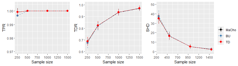
(a) Case 1

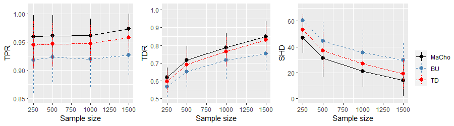
(b) Case 2

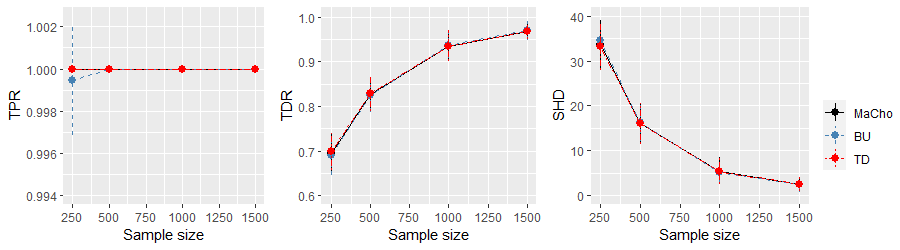
(c) Case 3

Figure 11: Comparison of the proposed algorithm MaCho, BU, and TD algorithms in terms of average TPR, TDR, and SHD for recovering linear SEM with different error variances and $p=20$.

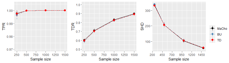
(a) Case 1

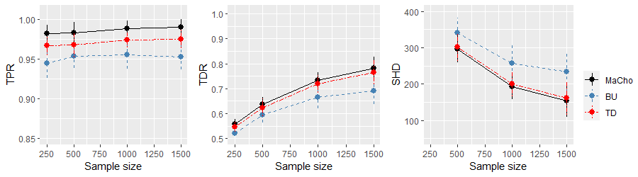
(b) Case 2

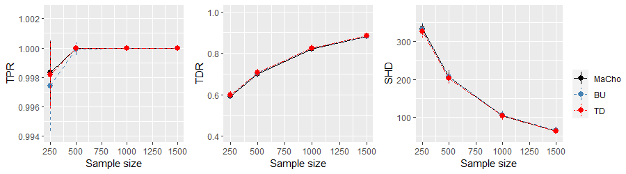
(c) Case 3

Figure 12: Comparison of the proposed algorithm MaCho, BU, and TD algorithms in terms of average TPR, TDR, and SHD for recovering linear SEM with different error variances and $p=50$.

References

• Basu et al. (2023) Basu, S., Das, S., Michailidis, G., and Purnanandam, A. A high-dimensional approach to measure connectivity in the financial sector. The Institute of Mathematical Statistics, 2023.
• Bertsekas (2015) Bertsekas, D. P. Convex Optimization Algorithms. Athena Scientific, 2015.
• Bien & Tibshirani (2011) Bien, J. and Tibshirani, R. J. Sparse estimation of a covariance matrix. Biometrika, 98(4):807–820, 2011. ISSN 00063444, 14643510.
• Billio et al. (2012) Billio, M., Getmansky, M., Lo, A. W., and Pelizzon, L. Econometric measures of connectedness and systemic risk in the finance and insurance sectors. Journal of Financial Economics, 104(3):535–559, 2012. ISSN 0304-405X. doi: https://doi.org/10.1016/j.jfineco.2011.12.010. Market Institutions, Financial Market Risks and Financial Crisis.
• Bollen (1989) Bollen, K. Structural Equations with Latent Variables. John Wiley and Sons, New York, 1989.
• Breiman (2001) Breiman, L. Random forests. Machine Learning, 45(1):5–32, 2001. doi: 10.1023/A:1010933404324.
• Cai et al. (2016) Cai, T. T., Ren, Z., and Zhou, H. H. Estimating structured high-dimensional covariance and precision matrices: Optimal rates and adaptive estimation. Electronic Journal of Statistics, 10:1–59, 2016.
• Chen et al. (2019) Chen, W., Drton, M., and Wang, Y. S. On causal discovery with an equal-variance assumption. Biometrika, 106(4):973–980, 09 2019. ISSN 0006-3444.
• Chickering (2003) Chickering, D. M. Optimal structure identification with greedy search. J. Mach. Learn. Res., 3(null):507–554, 2003. ISSN 1532-4435.
• Davis & Hager (2005) Davis, T. A. and Hager, W. W. Row modifications of a sparse cholesky factorization. SIAM Journal on Matrix Analysis and Applications, 26(3):621–639, 2005.
• Demirer et al. (2018) Demirer, M., Diebold, F. X., Liu, L., and Yilmaz, K. Estimating global bank network connectedness. Journal of Applied Econometrics, 33(1):1–15, 2018.
• Ghoshal & Honorio (2017) Ghoshal, A. and Honorio, J. Learning identifiable gaussian bayesian networks in polynomial time and sample complexity. In Advances in Neural Information Processing Systems, volume 30, 2017.
• Ghoshal & Honorio (2018) Ghoshal, A. and Honorio, J. Learning linear structural equation models in polynomial time and sample complexity. In Proceedings of the Twenty-First International Conference on Artificial Intelligence and Statistics, volume 84 of Proceedings of Machine Learning Research, pp.  1466–1475, 2018.
• Glymour et al. (2019) Glymour, C., Zhang, K., and Spirtes, P. Review of causal discovery methods based on graphical models. Frontiers in Genetics, 10, 2019. ISSN 1664-8021. doi: 10.3389/fgene.2019.00524. URL https://www.frontiersin.org/articles/10.3389/fgene.2019.00524.
• Golub & Van Loan (1996) Golub, G. H. and Van Loan, C. F. Matrix Computations (3rd Ed.). Johns Hopkins University Press, Baltimore, MD, USA, 1996. ISBN 0-8018-5414-8.
• Hardy et al. (1952) Hardy, G., Littlewood, J., and Pólya, G. Inequalities. Cambridge Mathematical Library. Cambridge University Press, 1952. ISBN 9780521358804.
• Horn & Johnson (2012) Horn, R. A. and Johnson, C. R. Matrix Analysis. Cambridge University Press, New York, NY, USA, 2nd edition, 2012.
• Hoyer et al. (2008) Hoyer, P. O., Janzing, D., Mooij, J., Peters, J., and Schölkopf, B. Nonlinear causal discovery with additive noise models. In Proceedings of the 21st International Conference on Neural Information Processing Systems, NIPS’08, pp.  689–696, 2008. ISBN 9781605609492.
• Janzing & Schölkopf (2010) Janzing, D. and Schölkopf, B. Causal inference using the algorithmic markov condition. IEEE Trans. Inf. Theor., 56(10):5168–5194, oct 2010. ISSN 0018-9448. doi: 10.1109/TIT.2010.2060095.
• Kalainathan & Goudet (2019) Kalainathan, D. and Goudet, O. Causal discovery toolbox: Uncover causal relationships in python, 2019.
• Khare et al. (2019) Khare, K., Oh, S.-Y., Rahman, S., and Rajaratnam, B. A scalable sparse cholesky based approach for learning high-dimensional covariance matrices in ordered data. Machine Learning, 108(12):2061–2086, 2019. doi: 10.1007/s10994-019-05810-5.
• Koller & Friedman (2009) Koller, D. and Friedman, N. Probabilistic Graphical Models: Principles and Techniques - Adaptive Computation and Machine Learning. The MIT Press, 2009. ISBN 0262013193.
• Loh & Bühlmann (2014) Loh, P.-L. and Bühlmann, P. High-dimensional learning of linear causal networks via inverse covariance estimation. Journal of Machine Learning Research, 15(88):3065–3105, 2014. URL http://jmlr.org/papers/v15/loh14a.html.
• Loh & Wainwright (2015) Loh, P.-L. and Wainwright, M. J. Regularized m-estimators with nonconvexity: Statistical and algorithmic theory for local optima. J. Mach. Learn. Res., 16(1):559–616, 2015. ISSN 1532-4435.
• Magnus & Neudecker (1986) Magnus, J. R. and Neudecker, H. Symmetry, 0-1 matrices and jacobians: A review. Econometric Theory, 2(2):157–190, 1986.
• Marshall et al. (2011) Marshall, A. W., Olkin, I., and Arnold, B. C. Inequalities: Theory of Majorization and its Applications, volume 143. Springer, second edition, 2011. doi: 10.1007/978-0-387-68276-1.
• Mooij et al. (2009) Mooij, J., Janzing, D., Peters, J., and Schölkopf, B. Regression by dependence minimization and its application to causal inference in additive noise models. In Proceedings of the 26th Annual International Conference on Machine Learning, ICML ’09, pp.  745–752, 2009. doi: 10.1145/1553374.1553470.
• Mooij et al. (2016) Mooij, J. M., Peters, J., Janzing, D., Zscheischler, J., and Schölkopf, B. Distinguishing cause from effect using observational data: Methods and benchmarks. J. Mach. Learn. Res., 17(1):1103–1204, jan 2016. ISSN 1532-4435.
• Olkin (1985) Olkin, I. Estimating a cholesky decomposition. Linear Algebra and its Applications, 67:201 – 205, 1985. ISSN 0024-3795.
• Park (2020) Park, G. Identifiability of additive noise models using conditional variances. Journal of Machine Learning Research, 21(75):1–34, 2020.
• Park & Park (2019) Park, G. and Park, H. Identifiability of generalized hypergeometric distribution (ghd) directed acyclic graphical models. In Chaudhuri, K. and Sugiyama, M. (eds.), Proceedings of the Twenty-Second International Conference on Artificial Intelligence and Statistics, volume 89 of Proceedings of Machine Learning Research, pp.  158–166. PMLR, 16–18 Apr 2019.
• Park & Raskutti (2018) Park, G. and Raskutti, G. Learning quadratic variance function (qvf) dag models via overdispersion scoring (ods). Journal of Machine Learning Research, 18(224):1–44, 2018.
• Peters & Bühlmann (2013) Peters, J. and Bühlmann, P. Identifiability of Gaussian structural equation models with equal error variances. Biometrika, 101(1):219–228, 11 2013. ISSN 0006-3444.
• Peters et al. (2011) Peters, J., Mooij, J. M., Janzing, D., and Schölkopf, B. Identifiability of causal graphs using functional models. In Proceedings of the Twenty-Seventh Conference on Uncertainty in Artificial Intelligence, UAI’11, pp.  589–598, Arlington, Virginia, USA, 2011. AUAI Press. ISBN 9780974903972.
• Peters et al. (2014) Peters, J., Mooij, J. M., Janzing, D., and Schölkopf, B. Causal discovery with continuous additive noise models. Journal of Machine Learning Research, 15(58):2009–2053, 2014. URL http://jmlr.org/papers/v15/peters14a.html.
• Peters et al. (2017) Peters, J., Janzing, D., and Schlkopf, B. Elements of Causal Inference: Foundations and Learning Algorithms. The MIT Press, 2017. ISBN 0262037319.
• Rajaratnam & Salzman (2013) Rajaratnam, B. and Salzman, J. Best permutation analysis. J. Multivar. Anal., 121:193–223, October 2013. doi: 10.1016/j.jmva.2013.03.001.
• Raskutti & Uhler (2013) Raskutti, G. and Uhler, C. Learning directed acyclic graphs based on sparsest permutations. Stat, 7, 07 2013. doi: 10.1002/sta4.183.
• Reisach et al. (2021) Reisach, A., Seiler, C., and Weichwald, S. Beware of the simulated dag! causal discovery benchmarks may be easy to game. In Ranzato, M., Beygelzimer, A., Dauphin, Y., Liang, P., and Vaughan, J. W. (eds.), Advances in Neural Information Processing Systems, volume 34, pp.  27772–27784. Curran Associates, Inc., 2021. URL https://proceedings.neurips.cc/paper_files/paper/2021/file/e987eff4a7c7b7e580d659feb6f60c1a-Paper.pdf.
• Shimizu et al. (2006) Shimizu, S., Hoyer, P. O., Hyvärinen, A., and Kerminen, A. A linear non-gaussian acyclic model for causal discovery. Journal of Machine Learning Research, 7(72):2003–2030, 2006.
• Shojaie & Michailidis (2010) Shojaie, A. and Michailidis, G. Penalized likelihood methods for estimation of sparse high-dimensional directed acyclic graphs. Biometrika, 97(3):519–538, 07 2010. doi: 10.1093/biomet/asq038.
• Simon (1977) Simon, H. A. Causal Ordering and Identifiability, pp.  53–80. Springer Netherlands, 1977. ISBN 978-94-010-9521-1. doi: 10.1007/978-94-010-9521-1˙5.
• Spirtes et al. (2001) Spirtes, P., Glymour, C., and Scheines, R. Causation, Prediction, and Search, 2nd Edition, volume 1 of MIT Press Books. The MIT Press, 2 edition, February 2001.
• Tao (2016) Tao, T. Analysis II. Singapore : Springer, third edition edition, 2016.
• Wainwright (2019) Wainwright, M. High-Dimensional Statistics: A Non-Asymptotic Viewpoint. Cambridge Series in Statistical and Probabilistic Mathematics. Cambridge University Press, 2019. ISBN 9781108498029.
• Wang (2014) Wang, H. Coordinate descent algorithm for covariance graphical lasso. Statistics and Computing, 24:521–529, 2014.
• Wang & Allen (2022) Wang, M. and Allen, G. I. Thresholded graphical lasso adjusts for latent variables. Biometrika, 110(3):681–697, 11 2022. ISSN 1464-3510. doi: 10.1093/biomet/asac060.
• Xue et al. (2012) Xue, L., Ma, S., and Zou, H. Positive-definite $\ell_{1}$-penalized estimation of large covariance matrices. Journal of the American Statistical Association, 107(500):1480–1491, 2012. doi: 10.1080/01621459.2012.725386.
• Yu & Bien (2017) Yu, G. and Bien, J. Learning local dependence in ordered data. Journal of Machine Learning Research, 18:1–60, 2017.
• Zhang & Spirtes (2015) Zhang, J. and Spirtes, P. The three faces of faithfulness. Synthese, 193:1011 – 1027, 2015.
• Zhang & Hyvärinen (2009) Zhang, K. and Hyvärinen, A. On the identifiability of the post-nonlinear causal model. UAI ’09, pp.  647–655, Arlington, Virginia, USA, 2009. AUAI Press. ISBN 9780974903958.
• Zhao & Yu (2006) Zhao, P. and Yu, B. On model selection consistency of lasso. J. Mach. Learn. Res., 7:2541–2563, dec 2006. ISSN 1532-4435.