Towards Optimal Circuit Size for Sparse Quantum State Preparation

Abstract

Compared to general quantum states, the sparse states arise more frequently in the field of quantum computation. In this work, we consider the preparation for $n$-qubit sparse quantum states with $s$ non-zero amplitudes and propose two algorithms. The first algorithm uses $O(ns/\log n+n)$ gates, improving upon previous methods by $O(\log n)$. We further establish a matching lower bound for any algorithm which is not amplitude-aware and employs at most $\operatorname{poly}(n)$ ancillary qubits. The second algorithm is tailored for binary strings that exhibit a short Hamiltonian path. An application is the preparation of $U(1)$-invariant state with $k$ down-spins in a chain of length $n$, including Bethe states, for which our algorithm constructs a circuit of size $O\left(\binom{n}{k}\log n\right)$. This surpasses previous results by $O(n/\log n)$ and is close to the lower bound $O\left(\binom{n}{k}\right)$. Both the two algorithms shrink the existing gap theoretically and provide increasing advantages numerically.

I Introduction

Quantum state preparation (QSP) is a crucial subroutine in various quantum algorithms, such as Hamiltonian simulation [1, 2, 3, 4] and quantum machine learning [5, 6, 7, 8, 9, 10, 11, 12, 13], to load classical data into a quantum computer. While preparing a general $n$-qubit quantum state requires $\Omega\quantity(2^{n})$ 1- and 2-qubit quantum gates [14], practical scenarios often involve structured classical data, allowing for a reduction in circuit size [15, 16, 17]. One typical example is sparse quantum state preparation (SQSP), where the data to be loaded is sparse. Sparse states are not only efficient to prepare but also hold practical significance. Many interesting quantum states are sparse, including the GHZ states, W states [18], Dicke states [19], thermofield double states [20], and Bethe states [21]. Moreover, several quantum algorithms specifically require sparse initial states, such as the quantum Byzantine agreement algorithm [22].

We briefly summarize previous work on SQSP. Gleinig et al. presented an efficient algorithm for SQSP by reducing the cardinality of basis states [15]. The Ref. [23] transformed SQSP to QSP by pivoting a sparse state into a smaller general state, which serves as a building block in their algorithm for constructing sparse isometries. In [24], the authors proposed the CVO-QRAM algorithm, whose cost depends on both the sparsity of the state and the Hamming weights of the bases. Decision diagrams have been employed in [25] to reduce circuit size for states with symmetric structures. Their algorithm also efficiently prepares sparse states. In [26], it was demonstrated that the Grover-Rudolph algorithm [27] for QSP is also efficient for SQSP, and gave an improvement based on a similar idea to [23]’s. While their techniques differ, the aforementioned algorithms require $\Theta\quantity(sn)$ 1- and 2-qubit gates to prepare an $n$-qubit states with $s$ non-zero entries in the worst case. On the other hand, the trivial lower bound of circuit size is $\Omega\quantity(s+n)$ with no better lower bound currently known to the best of our knowledge, leaving an open gap of $O\quantity(n)$. Additionally, there are efforts to reduce the circuit depth. [28] achieved a circuit depth of $\Theta(\log(sn))$ for SQSP at the expense of using $\mathcal{O}(sn\log s)$ ancillary qubits.

In this work, we aim at the optimizing circuit size for SQSP. We develop two algorithms within the framework of CVO-QRAM. The first algorithm achieves a circuit size of $O\quantity(\frac{ns}{\log n}+n)$, improving previous upper bound by a factor of $O\quantity(\log n)$. We show that our algorithm is asymptotically optimal under certain assumptions of SQSP algorithm. One of the assumptions, which is satisfied by previous SQSP algorithms, is that the algorithm must not be amplitude-aware. That is, the structure of the output circuit depends solely on the basis states rather than the amplitudes. The second algorithm performs better when the basis states can be efficiently iterated, achieving a circuit size of $O\quantity(L\log n)$, where $L$ is the number of bits flipped during iteration. This algorithm can be applied to prepare $U(1)$-invariant states, surpassing previous work by a factor of $O\quantity(\frac{n}{\log n})$. The comparison of our algorithms with previous ones is summarized in table I.

TABLE I: Comparison of circuit complexity for sparse state preparation and $U(1)$-invariant state preparation

Task	Algorithm	Circuit Size	#Ancilla
Sparse	[15]	$O(ns)$	0
	[23]	$O(ns)$	0
	[24]	$O(ns)$	0
	[25]	$O(ns)$	1
	[26]	$O(ns)$	0
	BE-QRAM	$O\quantity(\frac{ns}{\log n})$	2
$U(1)$	[36]	$O\quantity(\binom{n}{k}n)$	0
	LT-QRAM	$O\quantity(\binom{n}{k}\log n)$	$O(n)$

The remainder of the paper is structured as follows. In section II, we define terminology and give the problem formulation. In section III, we review the CVO-QRAM algorithm. In section IV, we introduce our first algorithm and proves its optimality under assumptions. In section V, we present our second algorithm and demonstrate its application to $U(1)$-invariant states. We conclude and discuss our results in section VII.

II Preliminary

Notations

Denote $[n]=\quantity{1,2,\dots,n}$. All logarithms $\log(\cdot)$ are base 2. For binary strings $x,y\in\quantity{0,1}^{n}$: $x_{i}$ is the $i$th bit of $x$; $\absolutevalue{x}$ means the Hamming weight of $x$; define $\overline{x}$ such that $\overline{x}_{i}=1-x_{i},\forall i\in[n]$; denote the bitwise XOR of $x,y$ by $x\oplus y$; define the corresponding $n$-qubit basis state as $\ket{x}$ and $\ket{x_{\quantity{i_{1},\dots,i_{k}}}}=\ket{x_{i_{1}},\dots,x_{i_{k}}}$. Denote the complex conjugate of $\alpha\in\mathbb{C}$ by $\alpha^{*}$.

(Sparse) quantum state

In a quantum system with $n$ qubits, the computational basis states are $2^{n}$ orthonormal vectors $\ket{0\dotsc 00},\ket{0\dotsc 01},\dotsc,\ket{1\dotsc 11}$, each identified as a binary string of length $n$. A general quantum state can be expressed as a normalized linear combination of these computational basis states:

$$\ket{\phi}=\sum_{x\in\quantity{0,1}^{n}}c_{x}\ket{x},\quad\sum_{x\in\quantity{0,1}^{n}}\absolutevalue{c_{x}}^{2}=1.$$ (1)

The coefficients $c_{x}$ are known as amplitudes. A quantum state is considered sparse if only a small fraction of its amplitudes are non-zero. The sparsity of a quantum state refers to the number of non-zero amplitudes. Call the set of binary strings corresponding to non-zero amplitudes the binary support of a sparse quantum state.

Quantum gate and quantum circuit

A $k$-qubit quantum gate is a $2^{k}\times 2^{k}$ unitary transformation that acts on a $k$-qubit subsystem. Our work utilizes the following quantum gates:

• The $X$ gate is a 1-qubit gate that flips a qubit between $\ket{0}$ and $\ket{1}$.

• The CNOT gate is a 2-qubit gate that applies an $X$ gate to the target qubit when the control qubit is $\ket{1}$.

• The Toffoli gate is a 3-qubit gate that applies an $X$ gate to a target qubit when the other two control qubits are both $\ket{1}$. It can be decomposed into 10 1-qubit gates and 6 CNOT gates [29].

• The $C^{t}X$ is a $(t+1)$-qubit gate that applies an $X$ gate to a target qubit when the other $t$ target qubits are all $\ket{1}$. This gate is known as a multi-controlled Toffoli gate, and can be decomposed into $O\quantity(n)$ 1-qubit gates and CNOT gates [30].

• The $G^{(\alpha,\beta)}$ gate is a 1-qubit gate with $\alpha\in\mathbb{C},\beta\in\mathbb{R}_{+}$ and $\absolutevalue{\alpha}\leq\beta$. It is defined as:

  $$G^{(\alpha,\beta)}=\frac{1}{\beta}\begin{pmatrix}-\sqrt{\beta^{2}-\absolutevalue{\alpha}^{2}}&\alpha\\ \alpha^{*}&\sqrt{\beta^{2}-\absolutevalue{\alpha}^{2}}\end{pmatrix}.$$ (2)

• The $C^{t}G^{(\alpha,\beta)}$ gate is a $(t+1)$-qubit gate that applies the $G^{(\alpha,\beta)}$ gate to a target qubit when the other $t$ target qubits are all $\ket{1}$. This gate can be decomposed into two 1-qubit gates and one multi-controlled Toffoli gate [31].

The qubits a gate acts on are indicated by writing their indices in the subscript of the gate. In the case of (multi-)controlled gates, the indices of the control qubits and the target qubit are separated by a semicolon. For example, $X_{j}$ represents the $X$ gate acting on the $j$th qubit, and $\operatorname{Tof}_{i,j;k}$ represents the Toffoli gate with the $i$th and $j$th qubit as controls and the $k$th qubit as the target.

An $n$-qubit quantum circuit is a sequence of quantum gates that implements a $2^{n}\times 2^{n}$ unitary transformation. The set of all 1-qubit gates and CNOT gates is considered universal because they can be used to implement any unitary transformation. For convenience, we refer to 1-qubit gates and CNOT gates as elementary gates. In our study, the size of a circuit is determined by the total number of elementary gates after decomposing all gates into elementary ones.

We will also encounter the concept of parameterized gates or circuit. A $k$-qubit parameterized gates are maps from some real or complex parameters to $2^{k}\times 2^{k}$ unitaries. For example, $G^{(\alpha,\beta)}$ and $C^{t}G^{(\alpha,\beta)}$ are said to be parameterized gates, if $\alpha,\beta$ are unspecified variables. Similarly, an $n$-qubit parameterized circuit is a sequence of (un)parameterized gates, that implements a map from some parameters to $2^{n}\times 2^{n}$ unitaries.

Problem formulation

In this work, we consider the preparation of sparse quantum states using quantum circuit with quantum elementary gates. Specifically, we are given a set of binary strings $S=\quantity{x^{j}\in\quantity{0,1}^{n}:1\leq j\leq s}$ of length $n$ with a size of $s$, and amplitudes $\quantity{c_{j}\in\mathbb{C}:1\leq j\leq s}$ satisfying $\sum_{j=1}^{s}\absolutevalue{c_{j}}^{2}=1$. Our goal is to output a quantum circuit $C_{S,\bm{c}}$ that prepares the $n$-qubit, $s$-sparse quantum state $\ket{\phi_{S,\bm{c}}}=\sum_{j=1}^{s}c_{j}\ket{x^{j}}$ using $m$ ancillary qubits, such that:

$$C_{S,\bm{c}}(\ket{0^{n}}\ket{0^{m}})=\ket{\phi_{S,\bm{c}}}\ket{0^{m}}.$$ (3)

Our objective is to minimize the size of the quantum circuit $C_{S,\bm{c}}$.

III Review of the CVO-QRAM algorithm

The CVO-QRAM algorithm [24] constructs a circuit of size $\Theta\quantity(\sum_{j=1}^{s}\absolutevalue{x^{j}})$ with one ancillary qubit to prepare any $n$-qubit $s$-sparse state $\ket{\phi}=\sum_{j=1}^{s}c_{j}\ket{x^{j}}$. In this section, we briefly review this algorithm. We will show how to improve upon this algorithm in the following sections.

CVO-QRAM loads the amplitudes and binary strings one by one in a specific order, utilizing one ancillary qubit to distinguish between loaded and being processed terms. Let $\ket{\bm{m}}_{\mathtt{M}}$ denote the $n$-qubit memory register, and $\ket{f}_{\mathtt{F}}$ denote the 1-qubit flag register. At the beginning of the algorithm, the registers are in the state $\ket{0^{n}}_{\mathtt{M}}\ket{1}_{\mathtt{F}}$. As proved in the following lemma, the algorithm deterministically transforms the registers into the state $\ket{\phi}_{\mathtt{M}}\ket{0}_{\mathtt{F}}$.

Lemma 1 (CVO-QRAM [24]).

Any $n$-qubit $s$-sparse state $\ket{\phi}=\sum_{j=1}^{s}c_{j}\ket{x^{j}}$ can be prepared using $\Theta\quantity(\sum_{j=1}^{s}\absolutevalue{x^{j}})$ elementary gates and one ancillary qubit.

Proof.

We may assume that $(c_{1},x^{1}),\dots,(c_{s},x^{s})$ are sorted such that $\absolutevalue{s^{j}}\leq\absolutevalue{s^{j+1}}$ for $1\leq j\leq s-1$. Let $\gamma_{j}:=\sqrt{1-\sum_{i=1}^{j-1}\absolutevalue{c_{i}}^{2}}$ for $1\leq j\leq s$. Algorithm 1 performs the transformation:

$$\ket{0^{n}}_{\mathtt{M}}\ket{1}_{\mathtt{F}}\to\ket{\phi}_{\mathtt{M}}\ket{0}_{\mathtt{F}}.$$ (4)

Input: $\quantity{(c_{j},x^{j})}_{1\leq j\leq s}$
Output: A circuit performing $\ket{0^{n}}_{\mathtt{M}}\ket{1}_{\mathtt{F}}\to\ket{\phi}_{\mathtt{M}}\ket{0}_{\mathtt{F}}$

For the $j$th string, with $1\leq j\leq s$:

1. $\ket{0^{n}}_{\mathtt{M}}\to\ket{x^{j}}_{\mathtt{M}}$ when $\ket{f}_{\mathtt{F}}=\ket{1}$.

2. Apply $C^{t}G^{(c_{j},\gamma_{j})}$ with controls on all $t=\absolutevalue{x^{j}}$ qubits where $x^{j}_{k}=1$ and target on $\ket{f}_{\mathtt{F}}$.

3. $\ket{x^{j}}_{\mathtt{M}}\to\ket{0^{n}}_{\mathtt{M}}$ when $\ket{f}_{\mathtt{F}}=\ket{1}$.

Algorithm 1 The CVO-QRAM algorithm.

We first prove the correctness of algorithm 1. It can be verified that at the beginning of the $j$th stage for $1\leq j\leq s$, the registers are in the following state:

$$\sum_{i=1}^{j-1}c_{i}\ket{x^{i}}_{\mathtt{M}}\ket{0}_{\mathtt{F}}+\gamma_{j}\ket{0^{n}}_{\mathtt{M}}\ket{1}_{\mathtt{F}}.$$ (5)

Hence, at the end of the algorithm, the registers will be in the state $\ket{\phi}_{\mathtt{M}}\ket{0}_{\mathtt{A}}$ with probability 1.

Next, let us analyze the circuit size. In the $j$th stage, the 1st and 3rd step can each be implemented by $\absolutevalue{x^{j}}$ CNOT gates, while the 2nd step can be implemented by $\Theta\quantity(\absolutevalue{x^{j}})$ elementary gates. Therefore, the entire circuit can be implemented by $\Theta\quantity(\sum_{j=1}^{s}\absolutevalue{x^{j}})$ elementary gates. ∎

We make two remarks regarding the CVO-QRAM algorithm.

1. The size of the constructed circuit is proportional to the number of 1s in all the $s$ binary strings. Hence, this algorithm excels when the state to prepare is double sparse, i.e., the state is sparse and the binary strings in the binary support have low Hamming weights. In the worst case, the circuit size of this algorithm is still $\Theta\quantity(sn)$. In the next section, we will demonstrate that the total number of 1s can be reduced for any set of binary strings, thus improving the worst case performance compared to CVO-QRAM.

2. The $G^{(c_{j},\gamma_{j})}$ gate has to be multi-controlled to ensure that the loaded terms are not affected. The straightforward solution is to apply the $G^{(c_{j},\gamma_{j})}$ gate when $\ket{\bm{m}}_{\mathtt{M}}=\ket{x^{j}}$. However, this implementation requires $\Theta\quantity(n)$ elementary gates. The trick employed by the CVO-QRAM algorithm is to sort the binary strings according to their Hamming weights, resulting in a reduction in the number of control qubits. The multi-controlled $G^{(c_{j},\gamma_{j})}$ will also be the bottleneck of our algorithms, and we will use different techniques to address it.

IV BE-QRAM

In this section, we present an enhanced version of the CVO-QRAM algorithm, which we refer to Batch-Elimation QRAM (BE-QRAM), that reduces the worst-case circuit size from $O\quantity(sn)$ to $O\quantity(sn/\log n)$. Additionally, we establish a corresponding lower bound for a specific class of algorithms.

As mentioned in the last section, the cost of the CVO-QRAM algorithm is propotional to the number of 1s in all the $s$ binary strings. To achieve this improvement, we eliminate 1s in the binary strings being prepared, leveraging the insight that any $\log_{2}(n)-\omega\quantity(1)$ binary strings have at most $o\quantity(n)$ distinct positions, as supported by the following lemma. It is worth noting that this observation has been previously utilized to optimize reversible circuits [32, 33].

Lemma 2.

Let $n,k,t,r\in\mathbb{N}$ where $k<\log n,t=2^{k},r=n-t$. Given $S_{k}=\quantity{y^{1},\dots,y^{k}}\subseteq\quantity{0,1}^{n}$, there exists an index set $\mathcal{T}\subseteq[n]$ of size $t$ such that for all $i\in\mathcal{R}=[n]\setminus\mathcal{T}$, there exists $j\in\mathcal{T}$ satisfying:

$$y_{i}^{p}=y_{j}^{p},\quad\forall p\in[k].$$ (6)

Furthermore, there exists a circuit $C$ consisting of $r$ CNOT gates that transforms $\ket{y^{p}}$ to $\ket{\hat{y}^{p}}$ for all $p\in[k]$, where $\hat{y}^{p}\in\{0,1\}^{n}$ and

$$\hat{y}_{i}^{p}=0,\quad\forall i\in\mathcal{R}.$$ (7)

Proof.

Let us call the length-$k$ binary string $y_{i}^{1}\dots y_{i}^{k}$ the pattern of $S_{k}$ at position $i$. Since there are at most $t=2^{k}$ distinct patterns, there exist $t$ patterns such that each of the remaining $r=n-t$ patterns coincides with one of them. We define $\mathcal{T}$ as the set of indices of these $t$ patterns.

For every $i\in\mathcal{R}$, let $l(i)$ be an index in $\mathcal{T}$ such that the pattern at position $l(i)$ coincides with the pattern at position $i$. It can be verified that the following CNOT circuit accomplishes the desired transformation:

$$C=\prod_{i\in\mathcal{R}}\operatorname{CNOT}_{l(i);i}.$$ (8)

∎

As an example, fig. 1 illustrates the CNOT circuit that eliminates 1s at the last 2 positions for 2 binary strings of length 6.

Figure 1: CNOT circuit eliminating 1s at the last 2 positions.

We are now ready to present our first algorithm. To begin with, we introduce parameters $k<\log_{2}n$, $t=2^{k}$, and $r=n-t$ as in lemma 2. The specific values for these parameters will be determined later. For simplicity, we assume that $k$ divides $s$ for now.

Our algorithm splits the $s$ binary strings into $\frac{s}{k}$ batches, where each batch contains $k$ strings. We will load these batches one by one, eliminating 1s in each batch following the method described in lemma 2. Moreover, to reduce the cost of multi-controlled $G^{(\alpha,\beta)}$ gates, we introduce an additional ancillary qubit compared to the CVO-QRAM algorithm. The detailed steps of the algorithm can be found in the proof of the following theorem.

Theorem 3.

An $n$-qubit $s$-sparse state can be prepared by a circuit of size $O\quantity(\frac{ns}{\log n}+n)$ with two ancillary qubits.

Proof.

Let $\ket{\phi}=\sum_{i=1}^{s/k}\sum_{j=1}^{k}c_{i,j}\ket{x^{i,j}}$ be the state to be prepared, and let

$$\gamma_{i,j}=\sqrt{1-\sum_{i^{\prime}=1}^{i-1}\sum_{j^{\prime}=1}^{k}\absolutevalue{c_{i^{\prime},j^{\prime}}}^{2}-\sum_{j^{\prime}=1}^{j-1}\absolutevalue{c_{i,j^{\prime}}}^{2}}.$$ (9)

In addition to the memory register $\ket{\bm{m}}_{\mathtt{M}}$ and the flag register $\ket{f}_{\mathtt{F}}$, we introduce an extra 1-qubit ancillary register $\ket{a}_{\mathtt{A}}$. Algorithm 2 performs the transformation

$$\ket{0^{n}}_{\mathtt{M}}\ket{0}_{\mathtt{A}}\ket{1}_{\mathtt{F}}\to\ket{\phi}_{\mathtt{M}}\ket{0}_{\mathtt{A}}\ket{0}_{\mathtt{F}}.$$ (10)

Input: $\quantity{(c_{j},x^{j})}_{1\leq j\leq s}$
Output: A circuit performing $\ket{0^{n}}_{\mathtt{M}}\ket{0}_{\mathtt{A}}\ket{1}_{\mathtt{F}}\to\ket{\phi}_{\mathtt{M}}\ket{0}_{\mathtt{A}}\ket{0}_{\mathtt{F}}$

For the $i$th batch, with $1\leq i\leq\frac{s}{k}$:

1. Apply the elimination circuit according to lemma 2, eliminating all 1s at positions $\mathcal{R}$ for binary strings in the $i$th batch. Recall that $\absolutevalue{\mathcal{R}}=r,\mathcal{T}=[n]\setminus\mathcal{R}$ and $\hat{x}^{i,j}$ denotes the eliminated form of string $x^{i,j}$.

2. $\ket{0}_{\mathtt{A}}\to\ket{1}_{\mathtt{A}}$ when $\ket{m_{\mathcal{R}}}_{\mathtt{M}}=\ket{0^{r}}$.

3. For the $j$th string in the $i$th batch, with $1\leq j\leq k$:

   1. $\ket{0^{n}}_{\mathtt{M}}\to\ket{\hat{x}^{i,j}}$ when $\ket{f}_{\mathtt{F}}=\ket{1}$.

   2. Apply $G^{(c_{i,j},\gamma_{i,j})}$ on $\ket{f}_{\mathtt{F}}$ when $\ket{m_{\mathcal{T}}}_{\mathtt{M}}=\ket{\hat{x}^{i,j}_{\mathcal{T}}}$ and $\ket{a}_{\mathtt{A}}=\ket{1}$.

   3. $\ket{\hat{x}^{i,j}}_{\mathtt{M}}\to\ket{0^{n}}$ when $\ket{f}_{\mathtt{F}}=\ket{1}$.

4. $\ket{1}_{\mathtt{A}}\to\ket{0}_{\mathtt{A}}$ when $\ket{m_{\mathcal{R}}}_{\mathtt{M}}=\ket{0^{r}}$.

5. Apply the reverse of the elimination circuit.

Algorithm 2 BE-QRAM

Let us first show the correctness of algorithm 2. Observe the following two facts:

• $\hat{x}^{i,j}$ are binary strings different from each other, since the elimination circuit is linear reversible.

• In step 3b, the conditions “$\ket{m_{\mathcal{T}}}_{\mathtt{M}}=\ket{\hat{x}^{i,j}_{\mathcal{T}}}$ and $\ket{a}_{\mathtt{A}}=\ket{1}$” is equivalent to “$\ket{\bm{m}}_{\mathtt{M}}=\ket{\hat{x}^{i,j}}$”.

From these observations, it can be verified that at the beginning of the $i$th batch, the registers are in the state:

$$\sum_{i^{\prime}=1}^{i-1}\sum_{j^{\prime}=1}^{k}c_{i^{\prime},j^{\prime}}\ket{x^{i^{\prime},j^{\prime}}}_{\mathtt{M}}\ket{0}_{\mathtt{A}}\ket{0}_{\mathtt{F}}+\gamma_{i,1}\ket{0^{n}}_{\mathtt{M}}\ket{0}_{\mathtt{A}}\ket{1}_{\mathtt{F}}.$$ (11)

Hence, at the end of the algorithm, the registers will be in the state $\ket{\phi}_{\mathtt{M}}\ket{0}_{\mathtt{A}}\ket{0}_{\mathtt{F}}$ with probability 1.

Next, we analyze the size of the constructed circuit.

• Step 1 and 5 can each be implemented by $r$ CNOT gates, according to lemma 2.

• Step 2 and 4 can each be implemented by $2r$ $X$ gates and one $C^{r}X$ gate, hence $O\quantity(r)$ elementary gates.

• Step 3a and 3c can each be implemented by $\absolutevalue{\hat{x}^{i,j}}\leq t$ CNOT gates.

• Step 3b can be implemented by $2(t-\absolutevalue{\hat{x}^{i,j}})\leq 2t$ $X$ gate and one $C^{t+1}G^{(c_{i,j},\gamma_{i,j})}$, hence $O\quantity(t)$ elementary gates.

In total, the circuit size is:

$$O\quantity(\left\lceil\frac{s}{k}\right\rceil(r+kt)).$$ (12)

By taking $k=\log n-\log\log n$, we get the desired size $O(\frac{ns}{\log n}+n)$. ∎

Next, we show that the $O\quantity(\frac{ns}{\log n}+n)$ size cannot be asymptotically reduced for a certain class of algorithms.

Theorem 4.

Suppose $s\leq 2^{\delta n}$ with $0\leq\delta<1$. If an algorithm $\mathcal{A}$ for preparing $n$-qubit $s$-sparse states satisfies the following conditions:

1. $\mathcal{A}$ uses at most $\operatorname{poly}\quantity(n)$ ancillary qubits.

2. $\mathcal{A}$ is not amplitude-aware, i.e., for any $S\subseteq\quantity{0,1}^{n}$ and $c:S\to\mathbb{C}$ describing the state, $\mathcal{A}$ outputs a parameterized circuit $U_{S}$ that depends only on $S$, along with parameters $\bm{\theta}_{S,c}$.

3. $U_{S}\neq U_{S^{\prime}}$ if $S\neq S^{\prime}$.

Then $\mathcal{A}$ requires $\Omega\quantity(\frac{ns}{\log n}+n)$ elementary gates in the worst case.

Proof.

We may assume that the circuit output by $\mathcal{A}$ is composed of CNOT and $R_{z},R_{y}$ gates, since single qubit gates admit ZYZ decomposition [29]. Let $K$ be the maximum circuit size, and suppose $\mathcal{A}$ uses at most $n^{C}$ qubits, where $C$ is a constant independent of $n$.

$\mathcal{A}$ can place a CNOT gate in $n^{C}(n^{C}-1)$ different ways, and place $R_{z},R_{y}$ in $n^{C}$ different ways each. Hence, the number of different $U_{S}$ can not exceed $\quantity(n^{C}(n^{C}-1)+2n^{C})^{K}$. On the other hand, the number of different $S$ is $\binom{n}{s}$. Therefore, by the assumption of $\mathcal{A}$, we have:

$$\quantity(n^{C}(n^{C}-1)+2n^{C})^{K} \geq\binom{2^{n}}{s}$$ (13)

$$\Longrightarrow K =\Omega\quantity(\frac{ns}{\log n}).$$ (14)

Since the state to prepare has $n$ qubits, we have $K=\Omega\quantity(n)$. Consequently, $K=\Omega\quantity(\frac{ns}{\log n}+n)$. ∎

Remark that the trivial lower bound of circuit size is $O\quantity(s+n)$, where $O\quantity(s)$ arises from the dimension, and $O\quantity(n)$ arises from the number of qubits. We are able to prove a non-trivial lower bound by imposing constraints to circuit generating algorithms. However, we believe that such constraints are reasonable, in a sense that they are satisfied by previous (sparse) quantum state preparation algorithms, except for the 1st constraint. We will elaborate on this point in the discussion section.

V LT-QRAM

In this section, we present another algorithm based on the CVO-QRAM algorithm, which we refer to as Lazy-Tree QRAM (LT-QRAM), that excels when the $s$ binary strings can be iterated in a loopless way. That is, there exists a procedure that generate these strings in sequence, such that the first one is produced in linear time and each subsequent string in constant time.

To this end, we introduce the concept of Hamiltonian path for a set of binary strings.

Definition 5.

Given a set $S\subseteq\quantity{0,1}^{n}$ of size $s$. Call an ordering of its elements $(x^{1},\dots,x^{s})$ a Hamiltonian path of $S$, and define the length of this path by $\sum_{j=2}^{s}\absolutevalue{x^{j-1}\oplus x^{j}}$.

Our second algorithm outputs a circuit whose size is linear in the length of a Hamiltonian path, multiplied by a factor of $O\quantity(\log n)$.

Theorem 6.

An $n$-qubit $s$-sparse state, whose binary support admits a Hamiltonian path of length $L$, can be prepared by a circuit of size $O\quantity(L\log n+n)$ with $O\quantity(n)$ ancillary qubits.

Proof.

Suppose $\ket{\phi}=\sum_{j=1}^{s}c_{j}\ket{x^{j}}$ is the state to be prepared, and $(x^{1},\dots,x^{s})$ is a Hamiltonian path of length $L$. Let $\gamma_{j}:=\sqrt{1-\sum_{i=1}^{j-1}\absolutevalue{c_{i}}^{2}}$ for $1\leq j\leq s$. For simplicity, we assume $n$ to be a power of 2. One can easily extend the proof for general $n$ without changing the asymptotic order.

In addition to the memory register $\ket{\bm{m}}_{\mathtt{M}}$ and the flag register $\ket{f}_{\mathtt{F}}$, we introduce an $n_{t}=2n-1$-qubit tree register $\ket{\bm{t}}_{\mathtt{T}}$ and an $n_{h}=\log_{2}n+1$-qubit ancillary register $\ket{\bm{h}}_{\mathtt{H}}$. $\ket{\bm{t}}_{\mathtt{T}}$ is structured as a full binary tree, whose leafs are in a one-to-one correspondence to the $n$ memory qubits $\ket{\bm{m}}_{\mathtt{M}}$. Denote the leaf qubit corresponding to $\ket{m_{i}}_{\mathtt{M}}$ by $\ket{q^{i}_{1}}_{\mathtt{T}}$, and its father, grandfather, et al., by $\ket{q^{i}_{2}}_{\mathtt{T}},\dots,\ket{q^{i}_{n_{h}}}_{\mathtt{T}}$. Hence, $\ket{q^{i}_{n_{h}}}_{\mathtt{T}}$ is the root of the tree for all $1\leq i\leq n$. Denote the sibling qubit of $\ket{q^{i}_{j}}_{\mathtt{T}}$ by $\ket{s^{i}_{j}}_{\mathtt{T}}$, for $1\leq j<n_{h}$. Define the depth of a qubit in $\ket{\bm{t}}_{\mathtt{T}}$ by the length of path from it to the root qubit, so that the $\ket{q^{i}_{j}}_{\mathtt{T}}$ has depth $n_{h}-j+1$. The layout of these registers and notations are illustrated in fig. 2, for the special case of $n=8$ and $i=5$.

Figure 2: Layout of registers $\ket{\bm{m}}_{\mathtt{M}}\ket{\bm{t}}_{\mathtt{T}}\ket{\bm{h}}_{\mathtt{H}}\ket{f}_{\mathtt{F}}$ in the proof of theorem 6. The lines are meant for visualization, rather than hardware topology.

Algorithm 3 performs the transformation

$$\ket{0^{n}}_{\mathtt{M}}\ket{0^{n_{t}}}_{\mathtt{T}}\ket{0^{n_{h}}}_{\mathtt{H}}\ket{1}_{\mathtt{F}}\to\ket{\phi}_{\mathtt{M}}\ket{0^{n_{t}}}_{\mathtt{T}}\ket{0^{n_{h}}}_{\mathtt{H}}\ket{0}_{\mathtt{F}}.$$ (15)

Input: $\quantity{(c_{j},x^{j})}_{1\leq j\leq s}$
Output: A circuit performing $\ket{0^{n}}_{\mathtt{M}}\ket{0^{n_{t}}}_{\mathtt{T}}\ket{0^{n_{h}}}_{\mathtt{H}}\ket{1}_{\mathtt{F}}\to\ket{\phi}_{\mathtt{M}}\ket{0^{n_{t}}}_{\mathtt{T}}\ket{0^{n_{h}}}_{\mathtt{H}}\ket{0}_{\mathtt{F}}$

1. $\ket{0^{n}}_{\mathtt{M}}\ket{0^{n_{t}}}_{\mathtt{T}}\to\ket{x^{1}}_{\mathtt{M}}\ket{1^{n_{t}}}_{\mathtt{T}}$.

2. Apply $G^{(c_{1},1)}$ to $\ket{f}_{\mathtt{F}}$.

3. For the $i$th string with $2\leq i\leq s$:

   1. $\ket{x^{i-1}}_{\mathtt{M}}\to\ket{x^{i}}_{\mathtt{M}}$ when $\ket{f}_{\mathtt{F}}=\ket{1}$.

   2. For each $j$ such that $x^{i-1}_{j}\neq x^{i}_{j}$:

      1. Apply $X_{h_{1}}$ when $\ket{f}_{\mathtt{F}}=\ket{0}$.

      2. For $2\leq k\leq n_{h}$, apply $\operatorname{Tof}_{h_{k-1},s^{j}_{k-1};h_{k}}$.

      3. For $1\leq k\leq n_{h}$, apply $\operatorname{CNOT}_{h_{k};q^{j}_{k}}$.

      4. Reverse step 3(b)i and 3(b)ii.

   3. Apply $G^{(c_{i},\gamma_{i})}$ when the root qubit of $\ket{\bm{t}}_{\mathtt{T}}$ is $\ket{1}$.

4. For $1\leq l<n_{h}$, and for each qubit of depth $l$th in the tree $\ket{\bm{t}}_{\mathtt{T}}$, apply a Toffoli gate with controls on its two children and target on itself.

5. For $1\leq j\leq n$, apply $X^{1-x^{s}_{j}}_{m_{j}}\operatorname{CNOT}_{m_{j};q^{j}_{1}}X^{1-x^{s}_{j}}_{m_{j}}$.

Algorithm 3 LT-QRAM

Let us first show the correctness of algorithm 3. It suffices to show that

1. At the start of the iteration of step 3, the registers are in the state:

   $$\sum_{i^{\prime}=1}^{i-1}c_{i^{\prime}}\ket{x^{i^{\prime}}}_{\mathtt{M}}\ket{\bm{t}(x^{i^{\prime}},x^{i-1})}_{\mathtt{T}}\ket{0^{n_{h}}}_{\mathtt{H}}\ket{0}_{\mathtt{F}}\\ +\gamma_{i}\ket{x^{i-1}}_{\mathtt{M}}\ket{1^{n_{t}}}_{\mathtt{T}}\ket{0^{n_{h}}}_{\mathtt{H}}\ket{1}_{\mathtt{F}}.$$ (16)

   Here, $\bm{t}(x,y)$ indicates that the tree register is an AND tree of whether segments of $x$ equals that of $y$. Formally, the leafs $\ket{q^{1}_{1}\dots q^{n}_{1}}_{\mathtt{T}}=\ket{\overline{x\oplus y}}$, and each interior qubit takes the value of the AND of its two children. Hence, the root qubit is $\ket{1}$ if and only if $x=y$.

2. Step 4 and 5 correctly uncompute the AND tree.

For the first point, the correctness of step 1 and 2 is obvious. We need to show that step 3b correctly updates the AND tree, after that the correctness of 3a and 3c is obvious. By changing $x^{i-1}$ to $x^{i}$, only paths ending in the root and starting at leaves that correspond to the differing bits between $x^{i-1}$ and $x^{i}$, need to be updated. Moreover, these paths can be updated in sequence. Consider the path $\ket{q^{j}_{1}}_{\mathtt{T}},\dots,\ket{q^{j}_{n_{h}}}_{\mathtt{T}}$. After step 3(b)i and 3(b)ii, we have that when $\ket{f}_{\mathtt{F}}=\ket{0}$,

$$\ket{h_{k}}_{\mathtt{H}}=\begin{cases}\ket{1},&k=1,\\ \ket{s_{1}\wedge\dots\wedge s_{k-1}},&k>1.\end{cases}$$ (17)

Then after step 3(b)iii, $\ket{q^{j}_{k}}_{\mathtt{T}}$ will be updated to $\ket{q^{j}_{k}\oplus h_{k}}$. It is not hard to verify that this is the desired update. When $\ket{f}_{\mathtt{F}}=\ket{1}$, $\ket{\bm{t}}_{\mathtt{T}}\ket{\bm{h}}_{\mathtt{H}}$ will not be changed. Hence, we have proven the first point. For the second point, first notice that before step 4, the registers are in the state:

$$\sum_{i=1}^{s}c_{i}\ket{x^{i}}_{\mathtt{M}}\ket{\bm{t}(x^{i},x^{s})}_{\mathtt{T}}\ket{0^{n_{h}}}_{\mathtt{H}}\ket{0}_{\mathtt{F}}.$$ (18)

After step 4, all interior qubits will be set to $\ket{0}$, by the definition of the AND tree. Since the leafs $\ket{q^{1}_{1},\dots,q^{n}_{1}}_{\mathtt{T}}=\ket{\overline{x^{i}\oplus x^{s}}}$ for $x^{i}$, step 5 will set all leafs to $\ket{0}$ too. Hence, we have proven the second point.

Next, we analyze the size of the constructed circuit.

1. Step 1 and 2 can be implemented by $\absolutevalue{x^{1}}+n_{t}+1=O\quantity(n)$ 1-qubit gates.

2. Step 3a can be implemented by $\absolutevalue{x^{i-1}\oplus x^{i}}$ CNOT gates.

3. Step 3b can be implemented by $O\quantity(\absolutevalue{x^{i-1}\oplus x^{i}}n_{h})=O\quantity(\absolutevalue{x^{i-1}\oplus x^{i}}\log n)$ elementary gates.

4. Step 3c can be implemented by $O(1)$ elementary gates.

5. Step 4 and 5 can be implemented by $O\quantity(n_{t})=O\quantity(n)$ elementary gates.

Recall the definition of $L$. In total, the circuit size is $O\quantity(L\log n+n)$. ∎

Since the circuit size is linear in $L$, one would be tempted to find the shortest Hamiltonian path given a set of binary strings. While this task is in general computationally hard [34] and the length of the shortest Hamiltonian path could be $\Theta\quantity(sn)$ [35], there are cases when there exists a short Hamiltonian path and the path is easy to compute. An example is the $U(1)$-invariant state [36], including Bethe state [21] and Dicke state [19] as a special case, whose binary support consists of all binary strings of Hamming weight $k$. As shown in the following corollary, in terms of circuit size, our algorithm outperforms a recent work for this task [36] by a factor $\frac{n}{\log n}$, and is nearly asymptotically optimal.

Corollary 7.

Any $U(1)$-invariant state $\sum_{x\in\quantity{0,1}^{n},\absolutevalue{x}=k}c_{x}\ket{x}$ can be prepared by a circuit of size $O\quantity(\binom{n}{k}\log n)$ with $O\quantity(n)$ ancillary qubits. Moreover, the classical complexity for generating the circuit is also $O\quantity(\binom{n}{k}\log n)$.

Proof.

For the $\binom{n}{k}$ binary string of Hamming weight $k$, there exists a Hamiltonian path of length $L=2\binom{n}{k}$ and the path can be computed in $O\quantity(L)$ classical time [37]. Hence, the corollary follows directly from theorem 6. ∎

VI Numerical results

We numerically test and benchmark our algorithms and present the results in fig. 3. Instead of circuit size, in the experiments we count the number of CNOT gates. Remark that usually the CNOT count is illustrative of circuit size [shende2004minimal], as is the case in our experiments. We benchmark our two algorithms separately, plotting the CNOT count against qubit numbers up to 6000.

Our first algorithm, the BE-QRAM algorithm, undergoes testing on randomly generated sparse states. To sample an $n$-qubit $s$-sparse state, we uniformly draw $s$ binary strings of length $n$ at random. Since the amplitudes do not influence circuit size for both our algorithm and previous ones, there is no need to sample amplitudes. We benchmark our algorithm and the CVO-algorithm, computing the CNOT count normalized by $(ns)^{-1}$ for varying $n$ and $s=n$. As depicted in fig. 3(a), the CNOT count of our algorithm fits well as $\Theta\quantity(\frac{ns}{\log n-\log\log n})$, while the CVO-QRAM algorithm scales as $\Theta\quantity(ns)$. Notice that after normalization, the cost of the CVO-QRAM algorithm remains constant for increasing $n$, while ours decreases.

Our second algorithm, the LT-QRAM algorithm, is examined on $U(1)$-invariant states. The binary support of a $U(1)$-invariant state with $k$ down-spins in a chain of length $n$ constitutes the set of all length-$n$ strings with a Hamming weight of $k$. Furthermore, there exists a minimal Hamiltonian path of length $2\binom{n}{k}$. Consequently, the circuit size of our algorithm admits a closed form dependent on $n$ and $k$. We benchmark our algorithm and the previous algorithm [36], computing the CNOT count normalized by $\quantity(\binom{n}{k}k)^{-1}$ for varying $n$ and $k=\left\lfloor\frac{n}{2}\right\rfloor$. As illustrated in fig. 3(b), the CNOT count of our algorithm fits well as $\Theta\quantity(\binom{n}{k}\log n)$, whereas [36] scales as $\Theta\quantity(\binom{n}{k}k)$. Notice that after normalization, the cost of [36] remains constant for increasing $n$, while ours decreases.

We implemented our algorithm in Python and ran the experiments on a 4.9 GHz Intel Core i7.

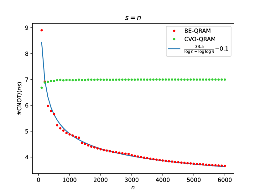
(a) $s$-sparse state

(b) $U(1)$-invariant state with $k$ down-spins

Figure 3: Benchmark of our algorithms on sparse states and $U(1)$-invariant states. We plot the “normalized” number of CNOT gates against the number of qubits $n$ up to 6000 for (a) $s$ sparse state with $s=n$; (b) $U(1)$-invariant state with $k=\left\lfloor n/2\right\rfloor$ down-spins. The red and green points represent the data of our algorithms and previous algorithms respectively, while the blue lines fit our data.

VII Conclusion and discussion

In this work, we propose two efficient algorithms for the task of sparse quantum state preparation, with a focus on optimizing circuit size. The first algorithm achieves a size of $O\quantity(\frac{ns}{\log n}+n)$, improving previous upper bound by a factor of $O\quantity(\log n)$. A matching lower bound is shown for any amplitude-unaware algorithms with moderate assumptions. The second algorithm is tailored for sparse states whose binary support admits a short Hamiltonian path, achieving a size of $O\quantity(L\log n)$, where $L$ is the length of the path. We show an application of the second algorithm to preparing $U(1)$-invariant state, including Bethe states, outperforming previous work by a factor of $O\quantity(n/\log n)$.

We are only able to prove the optimality of the first algorithm for a certain class of algorithms, rather than the problem itself. It remains open how to close the $O\quantity(s+n)$ vs $O\quantity(\frac{ns}{\log n}+n)$ gap. To the best of our knowledge, previous size lower bounds for quantum circuits are obtained via the dimensionality argument. That is, the number of continuous variables, hence the circuit size, cannot be fewer than the dimension of the problem. In terms of sparse quantum state preparation, such argument only gives a lower bound of $\Omega\quantity(s)$, which seems to contradict with the intuition that the choice of bases $S$ has an impact on efficiency. A possible bad case could be when the binary strings in $S$ differ from each other at $\Omega\quantity(n)$ positions, which is possible whenever $s=2^{\delta n},0\leq\delta<1$ by the Gilbert–Varshamov bound [35]. Based on our algorithmic lower bound, there could be 3 possibilities:

1. Either the true lower bound can be strengthened, which calls for new techniques for proving quantum circuit lower bounds.

2. Or, there exists better algorithms, which we believe must be amplitude-aware.

3. Or, there is a gap between the algorithmic and true lower bound, which means a compact circuit exists but is computationally hard to find.

We tend to believe the first case to be true.

Another interesting open question is to decide whether our second algorithm could be improved, especially for preparing $U(1)$-invariant states. In this special case, our algorithm is a factor of $O\quantity(\log n)$ away from the lower bound obtained by dimensionality argument. We believe this factor could be dropped.

References

- [1] D. W. Berry, A. M. Childs, R. Cleve, R. Kothari, and R. D. Somma, “Simulating hamiltonian dynamics with a truncated taylor series,” Physical review letters, vol. 114, no. 9, p. 090502, 2015.
- [2] G. H. Low and I. L. Chuang, “Optimal hamiltonian simulation by quantum signal processing,” Physical review letters, vol. 118, no. 1, p. 010501, 2017.
- [3] ——, “Hamiltonian simulation by qubitization,” Quantum, vol. 3, p. 163, 2019.
- [4] D. W. Berry, A. M. Childs, and R. Kothari, “Hamiltonian simulation with nearly optimal dependence on all parameters,” in 2015 IEEE 56th annual symposium on foundations of computer science. IEEE, 2015, pp. 792–809.
- [5] M. Schuld, I. Sinayskiy, and F. Petruccione, “An introduction to quantum machine learning,” Contemporary Physics, vol. 56, no. 2, pp. 172–185, 2015.
- [6] J. Biamonte, P. Wittek, N. Pancotti, P. Rebentrost, N. Wiebe, and S. Lloyd, “Quantum machine learning,” Nature, vol. 549, no. 7671, pp. 195–202, 2017.
- [7] I. Kerenidis and A. Prakash, “Quantum recommendation systems,” arXiv preprint arXiv:1603.08675, 2016.
- [8] P. Rebentrost, A. Steffens, I. Marvian, and S. Lloyd, “Quantum singular-value decomposition of nonsparse low-rank matrices,” Physical review A, vol. 97, no. 1, p. 012327, 2018.
- [9] A. W. Harrow, A. Hassidim, and S. Lloyd, “Quantum algorithm for linear systems of equations,” Physical review letters, vol. 103, no. 15, p. 150502, 2009.
- [10] L. Wossnig, Z. Zhao, and A. Prakash, “Quantum linear system algorithm for dense matrices,” Physical review letters, vol. 120, no. 5, p. 050502, 2018.
- [11] I. Kerenidis, J. Landman, A. Luongo, and A. Prakash, “q-means: A quantum algorithm for unsupervised machine learning,” Advances in neural information processing systems, vol. 32, 2019.
- [12] I. Kerenidis and J. Landman, “Quantum spectral clustering,” Physical Review A, vol. 103, no. 4, p. 042415, 2021.
- [13] P. Rebentrost, M. Mohseni, and S. Lloyd, “Quantum support vector machine for big data classification,” Physical review letters, vol. 113, no. 13, p. 130503, 2014.
- [14] M. Plesch and Č. Brukner, “Quantum-state preparation with universal gate decompositions,” Physical Review A, vol. 83, no. 3, p. 032302, 2011.
- [15] N. Gleinig and T. Hoefler, “An efficient algorithm for sparse quantum state preparation,” in 2021 58th ACM/IEEE Design Automation Conference (DAC). IEEE, 2021, pp. 433–438.
- [16] I. F. Araujo, C. Blank, and A. J. da Silva, “Entanglement as a complexity measure for quantum state preparation,” J, 2021.
- [17] A. G. Rattew and B. Koczor, “Preparing arbitrary continuous functions in quantum registers with logarithmic complexity,” arXiv preprint arXiv:2205.00519, 2022.
- [18] W. Dür, G. Vidal, and J. I. Cirac, “Three qubits can be entangled in two inequivalent ways,” Physical Review A, vol. 62, no. 6, p. 062314, 2000.
- [19] A. Bärtschi and S. Eidenbenz, “Deterministic preparation of dicke states,” in International Symposium on Fundamentals of Computation Theory. Springer, 2019, pp. 126–139.
- [20] W. Cottrell, B. Freivogel, D. M. Hofman, and S. F. Lokhande, “How to build the thermofield double state,” Journal of High Energy Physics, vol. 2019, no. 2, pp. 1–43, 2019.
- [21] J. S. V. Dyke, G. S. Barron, N. J. Mayhall, E. Barnes, and S. E. Economou, “Preparing bethe ansatz eigenstates on a quantum computer,” PRX Quantum, vol. 2, no. 4, p. 040329, 2021.
- [22] M. Ben-Or and A. Hassidim, “Fast quantum byzantine agreement,” in Proceedings of the thirty-seventh annual ACM symposium on Theory of computing, 2005, pp. 481–485.
- [23] E. Malvetti, R. Iten, and R. Colbeck, “Quantum circuits for sparse isometries,” Quantum, vol. 5, p. 412, 2021.
- [24] T. M. de Veras, L. D. da Silva, and A. J. da Silva, “Double sparse quantum state preparation,” Quantum Information Processing, vol. 21, no. 6, p. 204, 2022.
- [25] F. Mozafari, G. D. Micheli, and Y. Yang, “Efficient deterministic preparation of quantum states using decision diagrams,” Physical Review A, vol. 106, no. 2, p. 022617, 2022.
- [26] D. Ramacciotti, A.-I. Lefterovici, and A. F. Rotundo, “A simple quantum algorithm to efficiently prepare sparse states,” arXiv preprint arXiv:2310.19309, 2023.
- [27] L. Grover and T. Rudolph, “Creating superpositions that correspond to efficiently integrable probability distributions,” arXiv preprint quant-ph/0208112, 2002.
- [28] X.-M. Zhang, T. Li, and X. Yuan, “Quantum state preparation with optimal circuit depth: Implementations and applications,” Physical Review Letters, vol. 129, no. 23, p. 230504, 2022.
- [29] M. A. Nielsen and I. L. Chuang, Quantum computation and quantum information. Cambridge university press, 2010.
- [30] C. Gidney, “Constructing large controlled nots,” https://algassert.com/circuits/2015/06/05/Constructing-Large-Controlled-Nots.html, 2015.
- [31] A. Barenco, C. H. Bennett, R. Cleve, D. P. DiVincenzo, N. Margolus, P. Shor, T. Sleator, J. A. Smolin, and H. Weinfurter, “Elementary gates for quantum computation,” Physical review A, vol. 52, no. 5, p. 3457, 1995.
- [32] K. Markov, I. Patel, and J. Hayes, “Optimal synthesis of linear reversible circuits,” Quantum Information and Computation, vol. 8, no. 3&4, pp. 0282–0294, 2008.
- [33] D. V. Zakablukov, “On asymptotic gate complexity and depth of reversible circuits without additional memory,” Journal of Computer and System Sciences, vol. 84, pp. 132–143, 2017.
- [34] J. Ernvall, J. Katajainen, and M. Penttonen, “NP-completeness of the hamming salesman problem,” BIT Numerical Mathematics, vol. 25, pp. 289–292, 1985.
- [35] G. Cohen, S. Litsyn, and G. Zemor, “On the traveling salesman problem in binary hamming spaces,” IEEE Transactions on Information Theory, vol. 42, no. 4, pp. 1274–1276, 1996.
- [36] D. Raveh and R. I. Nepomechie, “Deterministic bethe state preparation,” arXiv preprint arXiv:2403.03283, 2024.
- [37] V. Vajnovszki and T. Walsh, “A loop-free two-close gray-code algorithm for listing k-ary dyck words,” Journal of Discrete Algorithms, vol. 4, no. 4, pp. 633–648, 2006.