Abstract

We calculate the quasinormal modes of a nonsingular spherically symmetric black hole effective model with holonomy corrections. The model is based on quantum corrections inspired by loop quantum gravity. It is covariant and results in a spacetime that is regular everywhere with a parameter-dependent black bounce.

Perturbations of these black holes due to massless scalar and electromagnetic fields have been previously calculated and some intriguing results were observed. For some modes, the frequency versus minimum-radius parameter trajectories were found to spiral and self-intersect in the complex plane. In addition, the spectrum of overtones has real frequencies that oscillate with increasing overtone number, and may even vanishing for some overtones.

We have calculated the quasinormal modes for all massless spin perturbations, including spin-1/2, and axial- and polar-gravitational. We find that the trajectory-spirals are restricted to scalar perturbations and observe some interesting overtone behaviour for gravitational perturbations. The amount of isospectrality violation in the gravitational quasinormal mode spectra is also examined.

1 Introduction

In the quest for a theory of quantum gravity, effective black hole models incorporating quantum corrections provide valuable insights. The paradigm of loop quantum gravity (LQG) has been useful for formulating some of these models [1, 2]. The LQG approach has been particularly successful in removing the black hole interior singularity with a bounce or transition surface. Obtaining consistent static exterior solutions that only exhibit quantum effects in regions of high-curvature is an active area of research [3, 4, 5, 6, 7, 8, 9, 10, 11, 12, 13, 14, 15, 16, 17].

We focus on the nonsingular spherically symmetric black hole effective model with holonomy corrections by Alonso-Bardaji, Brizuela, and Vera (ABV) [16, 17]. The model is based on quantum corrections inspired by loop quantum gravity. Anomaly-free holonomy corrections are included through a canonical transformation and a linear combination of constraints of general relativity. The construction is covariant and results in a spacetime that is regular everywhere with a parameter-dependent black bounce, and two asymptotically flat exterior regions. The quantum gravity effects introduce a length scale $r_{0}$. Curvature scalars are bounded everywhere, and quantum gravity effects die off with lower curvature. Schwarzschild spacetime is recovered for $r_{0}=0$ and Minkowski spacetime for vanishing black hole mass.

One possibility for confronting predicted quantum gravity effects is to study gravitational mergers. Gravitational mergers have been observed and can be conceptualised to occur in three stages: an initial inspiral, the merger, and a ringdown stage. Perturbation theory can be used to gain insight into the ringdown stage. A perturbed black hole is a dissipative system and gravitational waves are emitted as a spectrum of quasinormal modes (QNM) which act as the spectroscopy of the black hole. The amplitudes depend on the source of the oscillations, while the frequencies depend only on the black hole parameters. From now on, when we say QNMs, we mean the frequencies of the QNMs, not the amplitudes.

Gravitational wave (GW) data from merges is accumulating. Since the first gravitational waves were detected [18, 19], the LIGO-Virgo-KAGRA Collaborations have recorded 90 GW-burst events [20]. As a proliferation of possible black hole merger observations is anticipated, it is important to study black hole QNMs.

Planned improved sensitivity and efficiency of existing GW detectors, as well as the proposed new detectors LISA and the Einstein Telescope offer a bright future for our ability to deeply probe the gravitational domain. Continuous improvements may allow us to constrain new theories of gravity and possibly one day even shed light on some quantum aspects of gravity. One of the grand challenges in theoretical physics is to reconcile gravity with quantum mechanics.

QNMs from scalar perturbations of the ABV quantum corrected metric were first discussed in Ref. [21], and scalar and vector perturbations in Ref. [22]. In addition, gravitational lensing has been presented in Ref. [23, 24]. Some interesting QNM results have been obtained for scalar perturbations. As the distance parameter $r_{0}$ increases, the QNMs in the phase-space diagram self-intersect and spiral to a final extremal value. This was observed for the first two overtones $n=1,2$ for $s=\ell=0$ only, where $s$ is the spin of the perturbation and $\ell$ is the azimuthal number. No such curves were observed for $\ell=1$ or $\ell=2$, for $n=0,1,2$ [21]. Spirals were also not observed for electromagnetic perturbations [22]. We investigate if these spiral trajectories occur beyond the scalar $\ell=0$ overtones, and are inherent to the metric or the spin of the perturbation.

When studying high-overtones of scalar perturbations, the real part of the QNMs have been observed to oscillate with increasing overtone number. This behaviour has been observed for both $\ell=0$ and $\ell=1$ [21]. We address the question if such oscillations also occur for other spin perturbations.

The QNM spectra from axial- and polar-gravitational perturbations in general relativity are known to be identical [25, 26, 27, 28]. Such isospectrality is not anticipated for alternative metrics [29, 30, 31, 32, 33, 34]. We exam the amount of isospectrality violation in the ABV model for a few overtones and values of $\ell$.

This paper is structured as follows. In Section 2, the effective quantum corrected spacetime is summarised and stated to have many of the desired features of a quantum corrected asymptotically flat spacetime. The perturbation equations, potentials, and coordinates are introduced in Section 3 for the ABV line element and for spins $s=0,1/2,1,$ and $s=2$ (axial and polar) perturbations. The QNM boundary conditions for solving the eigenvalue problem are given in Appendix A, along with an asymptotic solution. The methods employed to calculated the QNMs are introduced in Section 4. The results are presented in Section 5 in terms of QNM phase-space trajectories, higher overtones, and isospectrality violation. For completeness, the first few overtones for all spins are presented as tables in Appendix B. We conclude with a discussion in Section 6.

Throughout, we work in geometric units of $G=c=1$. Without loss of generality, we take the usual $m=1/2$ $(r_{h}=1)$ in calculations.

2 Effective quantum corrected spacetime

The ABV model first writes the symmetry reduced Hamiltonian constraint and diffeomorphism constraint in terms of Asktekar-Barbero variables. These are the two densitized triads $\tilde{E}^{x}$ and $\tilde{E}^{\varphi}$, and their conjugate momentum $\tilde{K}_{x}$ and $\tilde{K}_{\varphi}$, where $x$ represents a radial coordinate and $\varphi$ an azimuthal coordinate. The holomony corrections are introduced by a polymerization procedure that replaces the conjugate momentum $\tilde{K}_{\varphi}$ with a periodic function $\sin(\lambda K_{\phi})/\lambda$. The dimensionless parameter $\lambda$ encodes the discretization of the quantum spacetime and is taken to be positive. However, to remain anomaly-free in the presence of matter, a canonical transformation is applied to the densitized triad variables and their conjugate momenta [35]:

$$\tilde{E}^{x}\to E^{x}\,,\quad\tilde{K}_{x}\to K_{x}\,,\quad\tilde{E}^{\varphi}\to\frac{E^{\varphi}}{\cos(\lambda K_{\varphi})}\,,\quad\text{and}\quad\tilde{K}_{\varphi}\to\frac{\sin(\lambda K_{\varphi})}{\lambda}\,.$$ (1)

This leaves the diffeomorphism constraint invariant provided $\cos(\lambda K_{\varphi})\neq 0$.

Since the surface $\cos(\lambda K_{\varphi})$ may vanish, a regularization procedure is applied by defining a linear combination of the Hamiltonian and diffeomorphism constraints [36]. General relativity is recovered from the new constraint for $\lambda\to 0$.

The new constraint algebra gives a structure function which vanishes at $E^{x}=0$, like in the Schwarzschild case, and for $\cos(\lambda K_{\varphi})=0$. From the definition of the constant of motion $m$, one obtains $\cos(\lambda K\varphi)=0$, if, and only if,

$$r_{0}\equiv\sqrt{E^{x}}=2m\frac{\lambda^{2}}{1+\lambda^{2}}\,,$$ (2)

where $m$ commutes on shell with the modified Hamiltonian. It is assumed that $m>0$ and $\lambda\neq 0$, which leads to $0<r_{0}<2m$. The classical theory is recovered in the limit $\lambda\to 0$, which implies $r_{0}\to 0$. The characteristic scale $r_{0}^{2}$ arises naturally from the constraint algebra and defines a minimum area of the model. The quantity $\cos(\lambda K_{\varphi})=0$ now covariantly defines surfaces on the manifold.

The metric functions are defined in terms of the phase-space variables in such a way that infinitesimal coordinate transformations on the spacetime coincide with the gauge variations on the phase space [37]. The covariance of the theory means the quantum effects do not depend on the particular gauge choice, which addresses criticisms raised in Ref. [38]. Satisfying these conditions, the line element is

$$ds^{2}=-N(r,x)^{2}dr^{2}+\left(1-\frac{r_{0}}{\sqrt{E^{x}(t,x)}}\right)^{-1}\frac{E^{\varphi}(t,x)^{2}}{E^{x}(t,x)}[dx+N^{x}(t,x)dt]^{2}+E^{x}(t,x)d\Omega^{2}\,,$$ (3)

where $d\Omega^{2}=d\theta^{2}+\sin^{2}\theta d\phi^{2}$ is the standard Riemannian metric on the unit radius 2-sphere, and $N(t,x)$ and $N^{x}(t,x)$ are the lapse and shift functions, respectively,

Different choices of gauge result in distinct charts and their corresponding line elements for the same metric. We limit our considerations to the static region of the quantum-corrected spacetime. This region is asymptotically flat and describes one exterior region. The gauge conditions $K_{\varphi}=0$ and $E^{x}=x^{2}$ are use to solve the equations of motion resulting in the ABV line element for the static region:

$$ds^{2}=-f(r)dt^{2}+\frac{1}{g(r)f(r)}dr^{2}+r^{2}d\Omega^{2},$$ (4)

with

$$f(r)=1-\frac{2m}{r}\quad\text{and}\quad g(r)=1-\frac{r_{0}}{r}\,,$$ (5)

where the event horizon radius is $r_{h}=2m$ and $r_{0}<2m$. Schwarzschild is restored in the limit $\lambda\to 0$.

Different geometric interpretations of the mass are possible. The addition of any function of $r_{0}$ to $m$ is also a constant of the motion. The constant of motion $m$ is neither the Komar, Hawking (Misner-Sharp), nor the ADM mass; $m$ is the Komar mass at spatial infinity and the Hawking mass at the horizon. We will express our results in terms of $m$ in correspondence with the Schwarzschild expression.

In addition, the Kretschmann scalar is always positive and finite for $r>r_{0}$. The bounce radius $r_{0}$ is hidden by the event horizon but quantum-gravity effects – parameterized by $r_{0}$ – are present outside the horizon, and decay as one moves to low-curvature regions. Some of these quantum-gravity effects are addressed in this paper.

One justifiable criticism of the ABV spacetime is the loss of contact with a quantum gravity origin [39]. If $\lambda$ is viewed to be a constant over the phase space, the value of $r_{0}$ is not fixed and increases as $m$ increases, as opposed to being fixed at some LQG minimum area.

3 Linear perturbations

Perturbations $\Psi_{s}$ of any spin can be written as a Schrödinger-like wave equation

$$\frac{\partial^{2}\Psi_{s}}{\partial r_{*}^{2}}+\left[\omega^{2}-V_{s}(r(r_{*}))\right]\Psi_{s}=0,$$ (6)

where $V_{s}$ is a spin-dependent effective potential, $r_{*}$ is the tortoise coordinate, and $\omega$ is a complex frequency.

The effective potentials for the ABV metric for $s=0,1,2$ (axial) and $s=1/2$ can be obtained from the general expressions in Ref. [40, 41, 42]:

$$V_{s}(r) = f(r)\left[\frac{\ell(\ell+1)}{r^{2}}+\frac{(1-s^{2})2m-(2s+1)(s-1)r_{0}/2}{r^{3}}\right.$$ (7)

$$\left.+\frac{(2s+3)(s-1)mr_{0}}{r^{4}}\right]\,,$$

$$V_{1/2}(r) = f(r)\left[\frac{(\ell+1)^{2}}{r^{2}}\pm(\ell+1)\sqrt{\frac{r-r_{0}}{r-2m}}\left(\frac{1}{r^{2}}-\frac{3m}{r^{3}}\right)\right],$$ (8)

where $\ell\geq s$ for integer $s$ and $\ell\geq 0$ for $s=1/2$. The case $s=2$ represents axial-gravitational perturbations: $V_{2}=V_{2}^{A}$. For polar-gravitational perturbations [34],

$$V_{2}^{P}(r)=\frac{f(r)}{6r^{4}}\frac{A(r)}{[r(4Lr+5r_{0})+2m(6r-7r_{0})]^{2}}\,,$$ (9)

where

$$A(r) = r^{3}\left(192L^{3}r^{3}+48L^{2}r^{2}(4r+5r_{0})+300Lrr_{0}^{2}+125r_{0}^{3}\right)$$

$$+12m^{2}r(6r-7r_{0})^{2}(4Lr+5r_{0})+6mr^{2}(6r-7r_{0})(4Lr+5r_{0})^{2}$$

$$+8m^{3}(6r-7r_{0})^{3}\,,$$

and $L=\ell(\ell+1)/2-1$.

For the ABV metric, the tortoise coordinated in Eq. (6), for $r_{0}\neq 2m$, is obtained from

$$\frac{dr_{*}}{dr}=\frac{1}{\sqrt{1-\frac{r_{0}}{r}}\left(1-\frac{2m}{r}\right)}=\sqrt{1-\frac{r_{0}}{r}}\left[1+\frac{4m^{2}}{(r-2m)(2m-r_{0})}-\frac{r_{0}^{2}}{(r-r_{0})(2m-r_{0})}\right]\,.$$ (11)

The former expression – actually, its reciprocal – will be used as the Jacobian in changes of variable. The later expression is a useful form for integration.

Less well defined is the integration to obtain $r_{*}$ as a function of $r$, since the constant of integration is arbitrary. We use the following integral

$$r_{*}(r) = \sqrt{1-\frac{r_{0}}{r}}\ r+\left(2m+\frac{r_{0}}{2}\right)\ln\left[\left(1+\sqrt{1-\frac{r_{0}}{r}}\,\right)^{2}\frac{r}{4}\right]$$ (12)

$$-\frac{2m}{\sqrt{1-\frac{r_{0}}{2m}}}\ln\left[\frac{\left(1+\sqrt{\left(1-\frac{r_{0}}{r}\right)\left(1-\frac{r_{0}}{2m}\right)}\,\right)^{2}2mr-r_{0}^{2}}{\left(1+\sqrt{1-\frac{r_{0}}{2m}}\,\right)^{2}2m(r-2m)}\right].$$

Constants have been included in the expression to reproduce the common Schwarzschild result for $r_{0}=0$, and to have no constants in the $r\to\infty$ and $r\to 2m$ limits, reproducing the results below. The complete $r_{*}(r)$ function is only need when plotting the potentials as a function of $r_{*}$; thus the potentials in $r_{*}$ include an arbitrary constant.

The asymptotic tortoise relation and coordinate can also be determined without knowing the exact form of the tortoise coordinate. For $r\to\infty$,

$$\frac{dr_{*}}{dr}\to\left(1+\frac{r_{0}}{2r}\right)\left(1+\frac{2m}{r}\right)\approx 1+\frac{2m+r_{0}/2}{r}\,,$$ (13)

$$r_{*}\approx r+\left(2m+\frac{r_{0}}{2}\right)\ln r\,.$$ (14)

For $r\to 2m$,

$$\frac{dr_{*}}{dr}\to\frac{2m}{\sqrt{1-\frac{r_{0}}{2m}}}(r-2m)^{-1}\,,$$ (15)

$$r_{*}\approx\frac{2m}{\sqrt{1-\frac{r_{0}}{2m}}}\ln(r-2m)\,.$$ (16)

These expressions will be useful when determining asymptotic solutions.

The potentials for various values of $r_{0}$ and the lowest values of $\ell$ are shown in Fig. 1; the next higher values of $\ell$ in Fig. 2. Direct comparison with previous results for $s=0$ and $s=1$ are not possible as those works do not state their expression for $r_{*}$. We notice the $s=\ell=0$ potentials appear distinct due to the absence of the centrifugal term $\ell(\ell+1)/r^{2}$. The $s=1$ potentials have the same maximum value since the potentials are independent of $r_{0}$, which only appears in the tortoise coordinate. The slow drop in the low-$r_{*}$ tail of most potentials is due to the high $r_{0}$ in the tortoise coordinate, which actually diverges for $r_{0}=r_{h}$. For $s=\ell=0$ and high values of $r_{0}$, the lower-$r_{*}$ tail in the potential falls faster than the other potentials due to the approximate cancellation of terms in the square bracket of Eq. (7).

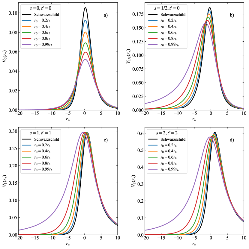
Figure 1: Potentials versus $r_{*}$ for a) spin-0, b) spin-1/2, c) spin-1, and d) spin-2 (axial) perturbations on the holonomy corrected black hole background metric for different values of $r_{0}$ and lowest values of $\ell$. A mass $m=1/2$ has been used.

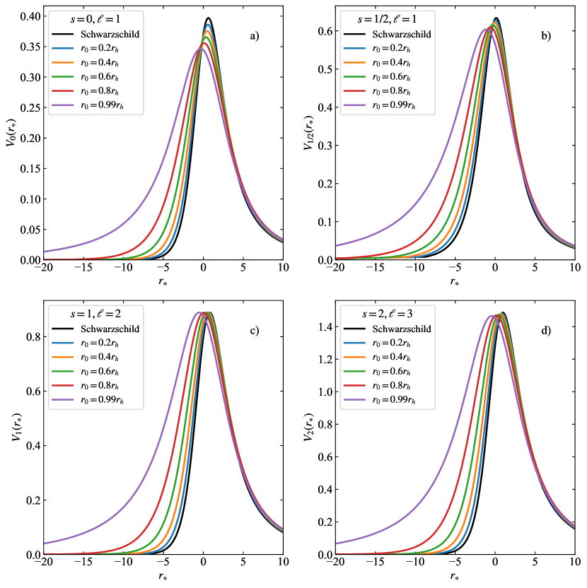
Figure 2: Potentials versus $r_{*}$ for a) spin-0, b) spin-1/2, c) spin-1, and d) spin-2 (axial) perturbations on the holonomy corrected black hole background metric for different values of $r_{0}$ and higher values of $\ell$. A mass $m=1/2$ has been used.

Figure 3 shows the polar-gravitational potentials. As expected, the axial- and polar-gravitational potentials differ by only a small amount.

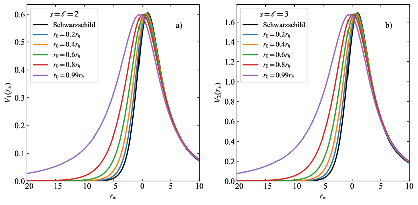
Figure 3: Polar-gravitational potentials versus $r_{*}$ for perturbations on the holonomy corrected black hole background metric: a) $\ell=2$ and b) $\ell=3$. A mass $m=1/2$ has been used.

4 Quasinormal mode frequency calculations

We will take advantage of three different methods for calculating QNMs. The semi-analytical Wentzel-Kramers-Brillouin (WKB) method which we use for all spin perturbations, but is limited in accuracy for high $n$ and low $\ell$. The pseudo-spectral method (PSM) will be used for low overtones, while the continued fraction method (CFM) will be employ for calculating higher overtones.

4.1 Wentzel-Kramers-Brillouin

The WKB method was first applied to the calculation of QNMs in Ref. [43], then developed to 3’rd-order in Ref. [44]. Although not particularly accurate for overtones, the method has the advantage of being semi-analytic and only requiring derivatives of the potential at the maximum.

The WKB method uses the following generic formula to calculation the QNM frequencies to order $p$:

$$\omega^{2}=V_{0}-i\sqrt{-2V_{0}^{\prime\prime}}\left[n+\frac{1}{2}+\sum_{i=2}^{p}\Lambda_{i}\right],\ \ n=0,1,\ldots\,,$$ (17)

where $V_{0}$ and $V_{0}^{\prime\prime}$ are $V(r_{*})$ and its second derivative calculated at the maximum of the potential, and $n$ is the overtone number. Each successive order contributes a term $\Lambda_{i}$ which is a function of higher derivatives of the potential evaluated at the maximum of the potential. Each successive term contributes to either the real or imaginary part of $\omega^{2}$. Higher order does not necessarily give better results.

In order to improve the WKB method, we employ the Padé approximation [45]. The 13’th-order WKB code with Padé approximation of Ref. [46] is used. We take the lowest relative uncertainty estimate to determine the optimal order of the calculation.

4.2 Pseudo-spectral method

In this section, we describe how we used the PSM to obtain QNMs. Spectral methods for solving differential equations are, in general, powerful and efficient provided the function is smooth, such as our case. The method approximates the solution we are trying to find, rather than the equation to be solved.

The Schrödinger-like equation (6) in $r_{*}$ is useful for applying the QNM boundary conditions, but its unbounded nature is not natural for numerical computations. We make a change of variable $u=2m/r$ to restrict the region outside the black hole $2m\leq r<\infty$ to $0<u\leq 1$. In addition, following the approach of Ref. [47], we applying the transformation

$$\Psi_{s}(u)=\frac{\Phi_{s}(u)}{u}e^{-i\omega r_{*}(u)}$$ (18)

to Eq. (6), giving

$$u^{3}(1-u)g(u)\Phi_{s}^{\prime\prime}(u)-u\left[\frac{u}{2}\left[1-g(u)-(1-3g(u))u\right]-4m\sqrt{g(u)}\ i\omega\right]\Phi_{s}^{\prime}(u)$$

$$+\left[\frac{u}{2}\left[1-g(u)-(1-3g(u))u\right]-\frac{(2m)^{2}V(r(u))}{u(1-u)}-4m\sqrt{g(u)}\ i\omega\right]\Phi_{s}(u)=0\,,$$ (19)

where primes represent derivatives with respect to $u$ and

$$g(u)=1-\frac{r_{0}}{2m}u\,.$$ (20)

Equation (19) would be the same result if we had started by writing the metric in Eddington-Filkenstein coordinates [47]. The Schwarzschild result is reproduced as $r_{0}\to 0$.

We now need to solve the above 2’nd-order ordinary differential equation (ODE) (19) with the proper boundary conditions. Substituting the following ansatz for the asymptotic solution

$$\Phi_{s}(u)=e^{4mi\omega/u}u^{-2(2m+r_{0}/2)i\omega}\phi_{s}(u)$$ (21)

into Eq. (19) gives

$$-\ (1-u)u^{3}g\phi_{s}^{\prime\prime}(u)$$

$$+\ \left\{\frac{1}{2}u^{2}\left[1-g-(1-3g)u\right]-4iu\left[\sqrt{g}-(3-g)g+(1-g)gu+2gu^{2}\right)\lambda\right\}\phi_{s}^{\prime}(u)$$

$$+\ \left\{-\frac{1}{2}u\left[1-g-(1-3g)u\right]+\frac{(2m)^{2}V}{u(1-u)}\right.$$

$$+\ i\left[-3+4\sqrt{g}-6g+g^{2}+(1-g)^{2}u+2(1-g)u^{2}\right]\lambda$$

$$\left.+\ 4\left[(-6\sqrt{g}+2g^{3/2}+9g-6g^{2}+g^{3})/u-4g(2-g)u-4gu^{2}\right]\lambda^{2}\right\}\phi_{s}(u)=0\,,$$ (22)

where $\lambda=\omega m$.

This is a quadratic eigenvalue problem in $\lambda$ (not the previous polymerization parameter). We have solved it using the pseudo-spectral code of Jansen [48]. The following is a brief description of what is implemented in the code and follows Ref. [47].

A quadratic eigenvalue equation can be written as

$$c_{0}(u,\lambda,\lambda^{2})\phi(u)+c_{1}(u,\lambda,\lambda^{2})\phi^{\prime}(u)+c_{2}(u,\lambda,\lambda^{2})\phi^{\prime\prime}(u)=0\,.$$ (23)

The coefficients can be written as $c_{j}(u,\lambda,\lambda^{2})=c_{j,0}(u)+\lambda c_{j,1}(u)+\lambda^{2}c_{j,2}(u)$. The regular function $\phi(u)$ is decomposed into cardinal functions $C_{j}(u)$,

$$\phi(u)=\sum_{j=1}^{N}y(u_{j})C_{j}(u)\,,$$ (24)

where $y(u)$ is a function of $u$. The differential equation and functions are evaluated at a set of points (grid)

$$u_{i}=\frac{1}{2}\left[1\pm\cos\left(\frac{i\pi}{N}\right)\right]\,,\quad i=0,1,2,\ldots,N\,,$$ (25)

where it has been written to map the interval $[-1,1]$ into $[0,1]$. Evaluation on a grid of collection points gives the pseudo-spectral method its name. This set of collection points is called the Gauss-Lobatoo grid.

Since the solution is not periodic and the domain is rectangular, combinations of Chebyshev polynomials of the first kind are the cardinal functions of choice:

$$C_{j}(u)=\frac{2}{Np_{j}}\sum_{m=0}^{N}\frac{1}{p_{m}}T_{m}(u_{j})T_{m}(u)\,,\quad p_{0}=p_{N}=2,p_{j}=1\,.$$ (26)

Evaluated on a grid, the coefficients $c_{j,0}(u_{i}),c_{j,1}(u_{i})$, and $c_{j,2}(u_{i})$ can be used to form a matrix:

$$\left(\tilde{M}_{0}+\tilde{M}_{1}\lambda+\tilde{M}_{2}\lambda^{2}\right)y=0\,,$$ (27)

where

$$(\tilde{M}_{0})_{ji} =c_{0,0}(u_{i})D_{ji}+c_{1,0}(u_{i})D_{ji}^{(1)}+c_{2,0}(u_{i})D_{ji}^{(2)}\,,$$ (28a)

$$(\tilde{M}_{1})_{ji} =c_{0,1}(u_{i})D_{ji}+c_{1,1}(u_{i})D_{ji}^{(1)}+c_{2,1}(u_{i})D_{ji}^{(2)}\,,$$ (28b)

$$(\tilde{M}_{2})_{ji} =c_{0,2}(u_{i})D_{ji}+c_{1,2}(u_{i})D_{ji}^{(1)}+c_{2,2}(u_{i})D_{ji}^{(2)}\,,$$ (28c)

and $D_{ji},D_{ji}^{(1)},D_{ji}^{(2)}$ are matrices of the cardinal function and its derivatives. Defining $\tilde{y}=\lambda y$,

$$\tilde{M}_{0}y+\left(\tilde{M}_{1}+\tilde{M}_{2}\lambda\right)\tilde{y}=0\,.$$ (29)

The matrix representation of the eigenvalue problem becomes

$$(M_{0}+M_{1}\lambda)\cdot\vec{y}=0\,,$$ (30)

where

$$M_{0}=\left(\begin{array}[]{cc}\tilde{M}_{0}&\tilde{M}_{1}\\ 0&1\end{array}\right)\,,\quad M_{1}=\left(\begin{array}[]{cc}0&\tilde{M}_{2}\\ -1&0\end{array}\right)\,,\quad\text{and}\quad\vec{g}=\left(\begin{array}[]{c}y\\ \tilde{y}\end{array}\right)\,.$$ (31)

Calculating QNM frequencies using the PSM does not depend on any initial guess, as in other methods. Unfortunately, the PSM leads to spurious solutions that do not have any physical meaning. The problem then becomes one of detecting and eliminating spurious solutions.

4.3 Continued fraction method

The CFM was first used to solve for QNMs by Leaver [49]. The method essential solves the differential equation by Frobenius method resulting in a set of algebraic recurrences relations, which are solved by continued fractions.

The Schrödinger-like wave equation (6) is simple in $r_{*}$ and is good for applying the boundary condition. However, because of the potential, it can be better to solve the equation in the variable $r$. The 2’nd-order ODE in $r$ becomes

$$(r-2m)(r-r_{0})\Psi_{s}^{\prime\prime}(r)+\frac{2m(r-r_{0})+(r_{0}/2)(r-2m)}{r}\Psi_{s}^{\prime}(r)+\frac{r^{3}}{r-2m}[\omega^{2}-V_{s}(r)]\Psi_{s}(r)=0\,,$$ (32)

which can be written in general as

$$P(r)\Psi_{s}^{\prime\prime}+Q(r)\Psi_{s}^{\prime}+R(r)\Psi_{s}=0\,,$$ (33)

where

$$P =(r-2m)(r-r_{0})\,,$$ (34a)

$$Q =\frac{2m(r-r_{0})+(r_{0}/2)(r-2m)}{r}\,,$$ (34b)

$$R =\frac{r^{3}}{r-2m}(\omega^{2}-V_{s}(r))\,.$$ (34c)

We postulate a series solution consisting of the asymptotic wave function $\psi(r)$, and the series approximation $\phi_{s}(r)$: $\Psi(r)=\psi(r)\phi_{s}(r)$. Applying the chain rule for $\Psi$ and substitution into Eq. (33) gives

$$P\psi\phi_{s}^{\prime\prime}+(2P\psi^{\prime}+Q\psi)\phi_{s}^{\prime}+(P\psi^{\prime\prime}+Q\psi^{\prime}+R$\mathrm{)}$\phi_{s}=0\,.$$ (35)

For the asymptotic solution, we take the form written in Ref. [21], which simplifies the recurrence relations relative to using the form presented in Appendix A:

$$\psi(r)=r(r-r_{0})^{i\omega(2m+r_{0}/2)-1}e^{i\omega r}\,.$$ (36)

The difference amounts to replacing $r$ by $r-r_{0}$ for some powers, which is allowed as $r\to\infty$.

In Eq. (32), regular singularities occur at $r=0$, $r=r_{0}$, and $r=2m$, while $r\to\infty$ is an irregular singularity. Following Ref. [21], the singularities at $(0,r_{0},2m,\infty)$ are mapped to $(2m/r_{0},\infty,0,1)$ by the change of variable

$$u=\frac{r-2m}{r-r_{0}}\,.$$ (37)

The domain $[2m,\infty]$, now maps to $[0,1]$ which is advantageous for numerical computation.

The variable $u$ is also the expansion variable in the Frobenius series. The derivatives of the series are ($r_{0}\neq 2m$)

$$\phi_{s}(u) =\sum_{n=0}^{\infty}a_{n}u^{\zeta+n}\,,$$ (38a)

$$\phi_{s}^{\prime}(u) =\frac{(1-u)^{2}}{2m-r_{0}}\sum_{n=0}^{\infty}a_{n}(\zeta+n)u^{\zeta+n-1}\,,$$ (38b)

$$\phi_{s}^{\prime\prime}(u) =\frac{(1-u)^{3}}{(2m-r_{0})^{2}}\sum_{n=0}^{\infty}a_{n}(\zeta+n)\left[(\zeta+n-1)(1-x)x^{\zeta+n-2}-2u^{\zeta+n-1}\right]\,,$$ (38c)

where primes now represent differentiation with respect to $u$. The characteristic exponent $\zeta$ is determined by the indicial equation and is found to be

$$\zeta=\frac{-i\omega(2m)^{3/2}}{\sqrt{2m-r_{0}}}\,.$$ (39)

The indicial equation corresponds to the ingoing solution at the horizon (see Appendix A).

For $s=0,1,2$ (axial), we obtain upon substitution of the series solution, the following four-term recurrence relations

$$\alpha_{0}a_{1}+\beta_{0}a_{0} =0\,,$$ (40a)

$$\alpha_{1}a_{2}+\beta_{1}a_{1}+\gamma_{1}a_{0} =0\,,$$ (40b)

$$\alpha_{n}a_{n+1}+\beta_{n}a_{n}+\gamma_{n}a_{n-1}+\delta_{n}a_{n-2} =0,\quad n=2,3,\ldots\,,$$ (40c)

where

$$\alpha_{n}= -8(n+1)i\omega(2m)^{5/2}(2m-r_{0})+4(n+1)^{2}(2m)(2m-r_{0})^{3/2}\,,$$ (41a)

$$\beta_{n}= \ 4\omega^{2}(2m)^{4}(2m-r_{0})^{1/2}+2[(12n+5)i\omega+6\omega^{2}(2m)](2m)^{5/2}(2m-r_{0})$$

$$-2[(6n^{2}+5n+2)+2[\ell(\ell+1)-s(s-1)]-3(2n+1)i\omega(2m)-6\omega^{2}(2m)^{2}]$$

$$\times(2m)(2m-r_{0})^{3/2}-2[(4n+1)i\omega-2\omega^{2}(2m)](2m)^{3/2}(2m-r_{0})^{2}$$

$$+2[2s+(2n+1)(n+i\omega(2m))](2m-r_{0})^{5/2}\,,$$ (41b)

$$\gamma_{n}= -8\omega^{2}(2m)^{4}(2m-r_{0})^{1/2}-4[(6n-1)i\omega+6\omega^{2}(2m)](2m)^{5/2}(2m-r_{0})$$

$$+[2(6n^{2}-2n+1)+4[\ell(\ell+1)-s(s-1)]-(24n-3)i\omega(2m)-17\omega^{2}(2m)^{2}]$$

$$\times(2m)(2m-r_{0})^{3/2}+4[(4n-1)i\omega+3\omega^{2}(2m)](2m)^{3/2}(2m-r_{0})^{2}$$

$$-2[(4n^{2}-2n+1)+2\ell(\ell+1)-s(2s-1)-(6n-1)i\omega(2m)-9\omega^{2}(2m)^{2}]$$

$$\times(2m-r_{0})^{5/2}+4\omega^{2}(2m)^{3/2}(2m-r_{0})^{3}$$

$$-[2s(2s+1)/(2m)-(4n-1)i\omega+\omega^{2}(2m)](2m-r_{0})^{7/2}\,,$$ (41c)

$$\delta_{n}= \ 4\omega^{2}(2m)^{4}(2m-r_{0})^{1/2}+2[(4n-3)i\omega+6\omega^{2}(2m)](2m)^{5/2}(2m-r_{0})$$

$$-2[2(2n^{2}-3n+1)-(12n-9)i\omega(2m)-5\omega^{2}(2m)^{2})(2m)(2m-r_{0})^{3/2}$$

$$-[(4n-3)i\omega+8\omega^{2}(2m)](2m)^{3/2}(2m-r_{0})^{2}$$

$$+[2(2n^{2}-3n+1)-4(4n-3)i\omega(2m)-15\omega^{2}(2m)^{2}](2m-r_{0})^{5/2}$$

$$+4\omega^{2}(2m)^{3/2}(2m-r_{0})^{3}-[2s(2s+1)/(2m)-(4n-3)i\omega-7\omega^{2}(2m)](2m-r_{0})^{7/2}$$

$$+[2s(2s+1)/(2m)^{2}-\omega^{2}](2m-r_{0})^{9/2}\,,$$ (41d)

The result agrees with Ref. [21] for $s=0$. Notice that all coefficients vanish as $r_{0}\to 2m$. The coefficients are at most quadratic in $\omega$ and the terms have dimension of mass to the 5/2 power. The $\sqrt{2m-r_{0}}$ factor comes from the inducial index.

The four-term recurrence relation is reduced to a three-term recurrence relation by applying Gaussian elimination [50]:

$$\tilde{\alpha}_{n}=\alpha_{n}\,,\quad\tilde{\beta}_{n}=\beta_{n}\,,\quad\tilde{\gamma}_{n}=\gamma_{n}\,,\quad\text{and}\quad\tilde{\delta}_{n}=0\,,\quad\text{for}\ n=0,1\,,$$ (42)

and

$$\tilde{\alpha}_{n}=\alpha_{n}\,,\quad\tilde{\beta}_{n}=\beta_{n}-\frac{\tilde{\alpha}_{n-1}\delta_{n}}{\tilde{\gamma}_{n-1}}\,,\quad\text{and}\quad\tilde{\gamma}_{n}=\gamma_{n}-\frac{\tilde{\beta}_{n-1}\delta_{n}}{\tilde{\gamma}_{n-1}}\,,\quad\text{for}\ n\geq 2\,.$$ (43)

The new variables now satisfies the three-term recurrence relation

$$\tilde{\alpha}_{0}a_{1}+\tilde{\beta}_{0}a_{0} =0\,,$$ (44a)

$$\tilde{\alpha}_{n}a_{n+1}+\tilde{\beta}_{n}a_{n}+\tilde{\gamma}_{n}a_{n-1} =0,\quad n=1,2,\ldots\,.$$ (44b)

The recurrence relations can be solved using a continued fraction. Writing Eq. (44b) as

$$\frac{a_{n}}{a_{n-1}}=\frac{-\tilde{\gamma}_{n}}{\tilde{\beta}_{n}+\tilde{\alpha}_{n}a_{n+1}/a_{n}}\,,$$ (45)

we substitution the left side into the right side an infinite number of times and use Eq. (44a) to give the continued fraction

$$0=\tilde{\beta}_{0}-\frac{\tilde{\alpha}_{0}\tilde{\gamma}_{1}}{\tilde{\beta}_{1}-}\frac{\tilde{\alpha}_{1}\tilde{\gamma}_{2}}{\tilde{\beta}_{2}-}\frac{\tilde{\alpha}_{2}\tilde{\gamma}_{3}}{\tilde{\beta}_{3}-}\cdots\,.$$ (46)

The $n$’th inversion of the continued fraction is

$$\tilde{\beta}_{n}-\frac{\tilde{\alpha}_{n-1}\tilde{\gamma}_{n}}{\tilde{\beta}_{n-1}-}\cdots-\frac{\tilde{\alpha}_{0}\tilde{\gamma}_{1}}{\tilde{\beta}_{0}}=\frac{\tilde{\alpha}_{n}\tilde{\gamma}_{n+1}}{\tilde{\beta}_{n+1}-}\frac{\tilde{\alpha}_{n+1}\tilde{\gamma}_{n+2}}{\tilde{\beta}_{n+2}-}\cdots$$ (47)

According to Ref. [49], the $n$’th inversion is the formula that should be used to solve for the $n$’th eigenfrequency. The left side of the $n$’th inversion is a finite continued fraction and is calculated using “back calculation” starting with $\tilde{\alpha}_{0}\tilde{\gamma}_{1}/\tilde{\beta}_{0}$. We have calculated the right side of the $n$’th inversion using the Nollert’s remainder.

Nollert [51] devised a method of improve on Leaver’s continued fraction method by estimating the remainder when truncating the back calculation. To get the Nollert method to work with four-term recurrence relations and Gaussian elimination, a large $n$ approximation of the tilde coefficients can be calculated.

We first obtain large $n$ asymptotic limits of the $\alpha_{n},\beta_{n},\gamma_{n}$, and $\delta_{n}$ coefficients by dividing their expressions by $n^{2}$ and keeping the first two terms in the expansion. Next we postulate the large-$n$ asymptotic expansion of $\tilde{\alpha}_{n},\tilde{\beta}_{n}$, and $\tilde{\gamma}_{n}$ to be of the form (also to 2’nd-order)

$$\tilde{\alpha}_{n} =r+u/n\,,$$ (48a)

$$\tilde{\beta}_{n} =s+v/n\,,$$ (48b)

$$\tilde{\gamma}_{n} =t+w/n\,.$$ (48c)

We then substitute the large-$n$ coefficients into the definitions (43) to obtain

$$\tilde{\alpha}_{n} =\ \ \ \ 8m(2m-r_{0})^{3/2}+u/n\,,$$ (49a)

$$\tilde{\beta}_{n} =-16m(2m-r_{0})^{3/2}+v/n\,,$$ (49b)

$$\tilde{\gamma}_{n} =\ \ \ \ 8m(2m-r_{0})^{3/2}+w/n\,,$$ (49c)

where

$$u =8[-i\omega(2m)^{5/2}(2m-r_{0})+(2m)(2m-r_{0})^{3/2}]\,,$$ (50a)

$$v =4[4i\omega(2m)^{5/2}(2m-r_{0})-2[1-3i\omega(2m)](2m)(2m-r_{0})^{3/2}$$

$$\ \ \ +i\omega(2m)(2m-r_{0})^{5/2}]\,,$$ (50b)

$$w =-4i\omega[2(2m)^{5/2}(2m-r_{0})+3(2m)^{2}(2m-r_{0})^{3/2}-(2m)(2m-r_{0})^{5/2}]\,.$$ (50c)

The recurrence relationship for the Nollert reminder is

$$R_{N}=\frac{\tilde{\gamma}_{N}}{\tilde{\beta}_{N}-\tilde{\alpha}_{N}R_{N+1}}\,,$$ (51)

which can be expanded as

$$R_{N}=C_{0}+C_{1}N^{-1/2}+C_{2}N^{-1}+\cdots\,.$$ (52)

The Nollert coefficients are

$$C_{0} = -1\,,$$ (53)

$$C_{1} = \pm\sqrt{2i(2m-r_{0})\omega}\,,$$ (54)

$$C_{2} = \frac{3}{4}-2i\left(2m-\frac{r_{0}}{4}\right)\omega\,.$$ (55)

We have validated our Nollert method by also using a straight back-calculation method and the modified Lentz’s method. In the limit of vary large number of fractions, back calculation and Nollert’s method should have the same accuracy. In the back-calculation method, for some large value of $N$ we take $\tilde{\alpha}_{N}=0$. This allows a backward calculation of the right side of the $n$’th inversion back to the fraction containing $\tilde{\alpha}_{n}\tilde{\gamma}_{n+1}/\tilde{\beta}_{n+1}$. A good approximation method for evaluating continued fractions is the modified Lentz’s method [52]. It is based on relating continued fractions to rational approximations, and allows a simple test of how much the result changes from one iteration to the next.

For any of the three methods, the resulting equation in $\omega$ must be solved by root-finding. A guess for the root is obtained by linear extrapolating using the current $\omega_{n}$ and the change giving by the difference between the current $\omega_{n}$ and the previous $\omega_{n-1}$. An approximation to the $n=0$ mode is used as the initial guess.

5 Results

We present QNMs on a phase diagram versus the quantum parameter $r_{0}$, higher overtones for different values of $r_{0}$, and isospectrality violation by examining the difference in QNMs of axial- and polar-gravitational perturbations. When referring to the Schwarzschild value, $r_{0}=0$ is used in the ABV calculations.

5.1 Trajectories

We first study how the QNMs change for different values of $r_{0}$. Figure 4 shows phase diagrams or trajectories for $r_{0}=[0,0.99]$ for $s=\ell=0$ and $n=1,2,3$, and $r_{0}=[0,0.9]$ otherwise. The CFM and PSM were used for $s=0,1,2$ (axial), and WKB method for $s=1/2$. The PSM was also used for $s=2$ (polar). The CFM calculations are shown in black, red, and blue. Underneath these curves the PSM calculations are shown in magenta. In some cases the CFM and PSM are similar enough that the PSM curves are not visible. The difference between the two method of calculation are most apparent for large $r_{0}$. In the $s=2$ plot, the PSM calculations of the polar modes are shown underneath in green.

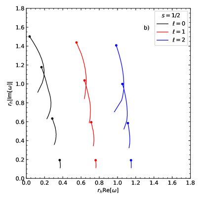
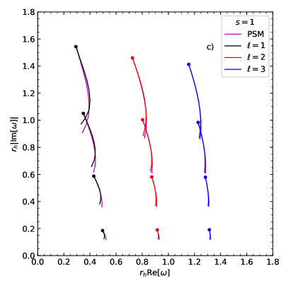
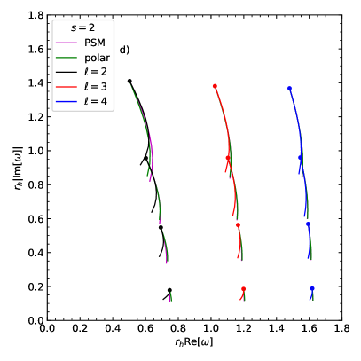
Figure 4: First four ($n=0,1,2,3$) QNMs from bottom to top for $r_{0}=0$ to 0.9 (0.99 for spirals). a) $s=0$ and $\ell=0,1,2$ from left to right, b) $s=1/2$ and $\ell=0,1,2$ from left to right, c) $s=1$ and $\ell=1,2,3$ from left to right, and d) $s=2$ and $\ell=2,3,4$ from left to right. The top points of each curve are the Schwarzschild values. A mass of $m=1/2$ has been used.

For $s=0$, we reproduce the results of Ref. [21] and continue them to overtone $n=3$. The $s=1$ and $s=2$ results are new, although for $s=1$ Ref. [22] plotted the real and imaginary parts of $\omega$ separately. The self-intersecting spirals continue for $s=\ell=0$. We do not observe any additional self-intersecting spirals beyond those.

The trajectories using two different numerical methods agree well for $s=0$ in the non-spiral cases. The agreement is less good for $s=1$ and $s=2$. However, the agreement improves as $\ell$ increases. It’s clear that the CFM determines the self-intersecting spirals better than the PSM. The $s=1/2$ trajectories are unlikely to be particularly accurate for $n>\ell$.

Self-intersecting and non-intersecting spiral trajectories have been previously observed for Reissner-Nordström and Kerr black holes [50, 53, 54], as well as modified gravity black holes [55, 56].

5.2 Higher overtones

The ABV metric is very close to Schwarzschild everywhere, except for a small region near the event horizon, which is crucial for overtones [57]. Figures 5, 6, and 7 show higher overtones using the CFM. Based on the trajectory agreement between the PSM and CFM for low values of $r_{0}$, we only consider $r_{0}\leq 0.5$ when calculating the higher overtones. We have assumed symmetry in the real part of $\omega$ and drawn identical points on both sides of the imaginary axis.

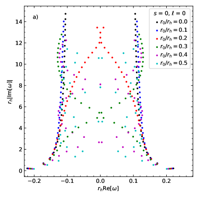
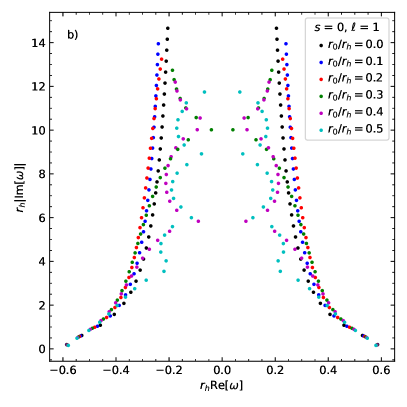
Figure 5: First 30 QNMs $(n=0,1,\ldots 29)$ for scalar perturbations on a holonomy corrected black hole background a) $s=0,\ell=0$ and b) $s=0,\ell=1$, The continued fraction method with mass $m=1/2$ was used.

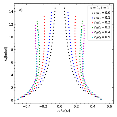
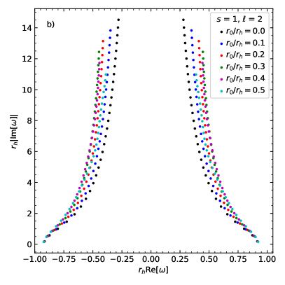
Figure 6: First 30 QNMs $(n=0,1,\ldots 29)$ for vector perturbations on a holonomy corrected black hole background a) $s=1,\ell=1$ and b) $s=1,s=2$. The continued fraction method with mass $m=1/2$ was used.

For $s=0$ (Fig. 5), we reproduce the results in Ref. [21]. For $s=1$ (Fig. 6) and $s=2$ (axial) (Fig. 7), the results are new. For $s=1$, within the number of modes consider, no oscillations or pure imaginary modes are observed.

Interesting behaviour is observed for $s=2$ (Fig. 7). Purely imaginary modes occur above the, well known, Schwarzschild purely imaginary modes for small values of $r_{0}$. It seems likely that pure imaginary modes will occur for other values of $r_{0}$. As $r_{0}$ increases the trend is similar to the $s=1$ perturbations, and it is not clear if purely imaginary modes will occur at very high overtones. No multiple oscillations are observed for $s=2$ over the number of overtones we calculate.

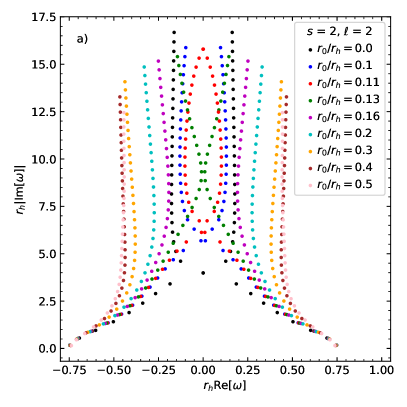
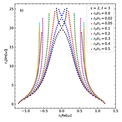
Figure 7: Higher overtones for axial-gravitational perturbations on a holonomy corrected black hole background a) first 34 QNMs $(n=0,1,\ldots 33)$, $s=2$ (axial), $\ell=2$ and b) first 51 QNMS $(n=0,1,\ldots 50)$, $s=2$ (axial), $\ell=3$. The continued fraction method with mass $m=1/2$ was used.

5.3 Isospectrality

If the QNM frequency spectrum from axial- and polar-gravitational perturbations are the same, this property is referred to as isospectrality. Isospectrality for Schwarzschild and Reissner-Nordström metrics have been proven [25, 26]. Isospectrality has also been demonstrated to linear order in the spin for Kerr black holes [27, 28], and for Schwarzschild-de Sitter and Schwarzschild-anti de Sitter spacetimes [58]. However, isospectrality appears not to be a universal feature that holds for modified gravity spacetimes [29, 30, 31, 32, 33, 34]. It is thus important to compare the spectra for gravitational perturbations on the ABV black hole background.

Figure 8 shows the difference between the axial $\omega_{A}$ and polar $\omega_{P}$ gravitational quasinormal mode frequencies versus $r_{0}$ on the ABV black hole background. The difference in the real and imaginary parts are shown as solid and dashed lines, respectively. Schwarzschild isospectrality was obtained to better than seven digits. The maximum violation of isospectrality is observed to not necessarily occur at the extremal value of $r_{0}=r_{h}$. The amount of isospectrality violation, in general, increases with overtone number. The case of fundamental mode $n=0$ for $\ell=2$ shows nonmonotonic variation in the real part relative to the overtones and the fundamental for higher values of $\ell$. The amount of isospectrality violation decreases with increasing $\ell$. The violation of isospectrality is about a factor of 0.3 for $\ell=3$ relative to $\ell=2$, and then again a factor of about 0.5 for $\ell=4$ (not shown) relative to $\ell=3$ .

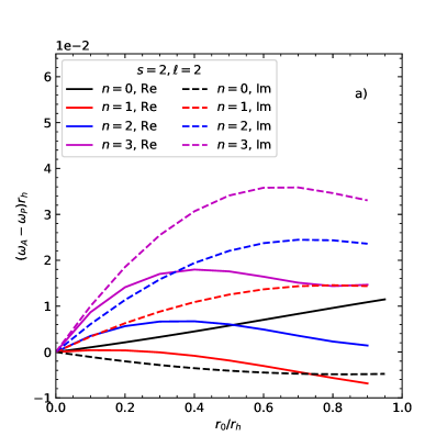
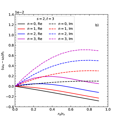
Figure 8: Difference between the axial- and polar-gravitational quasinormal mode frequencies versus $r_{0}$ on a holonomy corrected black hole background. The difference in the real and imaginary parts are shown as solid and dashed lines, respectively. The pseudo-spectral method with mass of $m=1/2$ has been used.

6 Discussion

We have plotted the QNMs versus $r_{0}$ on a phase-space diagram for $s=0,1,2$ and $\ell=s,s+1,s+2$ for $n=0,1,2,3$. As well as, $s=1/2$, for $\ell=0,1,2$. Only the $s=\ell=0$, $n=1,2,3$ modes exhibit self-intersecting spirals. We postulate that such behaviour is unlikely to be a universal property of the ABV metric but more associated to the unique shape of the potentials for $s=0$. Such behaviour has previously been observed, for example, in Reissner-Nordström spacetime [50]. The ABV behaviour may not be unexpected if we interpret the Reissner-Nordström mass and charge to be $M=m+r_{0}/2$ and $Q^{2}=2mr_{0}$, respectively [17].

We now discuss the trajectories in terms of the polymerization approach. Recall that $r_{0}$ given by Eq. (2) is proportional to the constant of the motion $m$, and $\lambda$ is a real dimensionless parameter, which can be taken without loss of generality to be positive. It encodes the discretization of the quantum spacetime and is related to the length of the holonomies. We can consider $\lambda$ a universal constant over the entire phase space in which case the trajectories will depend on $\lambda$. Or, we can consider $\lambda$ a constant of the solution, in which the trajectories will depend on $r_{0}$. The trajectory plots support either interpretation, although in the first interpretation it should be understood that $\lambda$ is varying along the trajectory, not $r_{0}$ as mentioned in the figure captions.

Higher overtones for $s=0,1,2$ (axial) and for $\ell=s$ and $\ell=s+1$ are calculated. The $s=0$ behaviour first observed in Ref. [21] is reproduced. For $s=1$, there appears to be no case of near vanishing oscillating modes. However, for axial-gravitational perturbations a rich pattern of overtones is observed for $\ell=2$. In this case, we are probing beyond the first crossing of the imaginary axis. For $\ell=3$, oscillations in the real part of the QNMs may occur for very high overtones.

Isospectrality is clearly violated for gravitational perturbations on a ABV black hole background. In general, the amount of violation increases with increasing overtone number and decreases with increases $\ell$. The amount of isospectrality violation is not always monotonically increasing with increasing $r_{0}$, and is not, in general, a maximum or minimum at the extremal values of $r_{0}=r_{h}$.

Appendix A Boundary conditions and an asymptotic solution

In this appendix we discuss the QNM boundary conditions and write down an asymptotic solution. The aim is to solve the Schrödinger-like wave equation (6) for the complex eigenfrequencies $\omega$. The potential is zero at the horizon and at spatial infinity, and the Schrödinger-like equation becomes a harmonic oscillator problem. The boundary condition at the horizon is a wave that purely goes into the black hole; representing classically that nothing comes out. The other boundary condition at spatial infinity is a wave that purely goes out; as nothing comes from outside the spacetime. The boundary condition at spatial infinity is given as $r\to\infty$, $r_{*}\to r+(2m+r_{0}/2)\ln r$, which gives

$$\psi^{r\to\infty}\to e^{i\omega r_{*}}\to r^{i\omega(2m+r_{0}/2)}e^{i\omega r}\,.$$ (56)

Normalized to unity at the horizon, we write

$$\psi^{r\to\infty}_{r\to r_{h}}\to r^{i\omega(2m+r_{0}/2)}e^{i\omega(r-2m)}\,.$$ (57)

The boundary condition at the event horizon is given as $r\to 2m$ ($r_{0}\neq 2m$),

$$r_{*}\to\frac{2m}{\sqrt{1-\frac{r_{0}}{2m}}}\ln(r-2m)\,,$$ (58)

which gives

$$\psi^{r\to r_{h}}\to e^{-i\omega r_{*}}\to(r-2m)^{\zeta}\,,$$ (59)

where

$$\zeta=\frac{-i\omega(2m)^{3/2}}{\sqrt{2m-r_{0}}}\,.$$ (60)

Normalized to unity at spatial infinity, we write

$$\psi^{r\to r_{h}}_{r\to\infty}\to e^{-i\omega r_{*}}\to(r-2m)^{\zeta}r^{-\zeta}\,.$$ (61)

Combining the two asymptotic solutions, we form the asymptotic wave function satisfying both boundary conditions

$$\psi(r)=r^{i\omega(2m+r_{0}/2)-\zeta}(r-2m)^{\zeta}e^{i\omega(r-2m)}\,.$$ (62)

The boundary conditions do not depend explicitly on $s$ or $\ell$, so the above solution can be used for all spin and angular momentum perturbations.

Appendix B Tables of quasinormal mode frequencies

The following tables show some QNM frequencies for all integer spins for $\ell=s$ and $\ell=s+1$, and spin-1/2 for $\ell=0$ and $\ell=1$. The fundamental and first few overtones are shown for the cases of $r_{0}=0$ (Schwarzschild), and $r_{0}=0.3r_{h}$ and $r_{0}=0.5r_{h}$ ABV. The WKB method has been used in the first two line of each table ($n=0,1$). Also shown in the middle section of each table, except for the cases of $s=1/2$, are the fundamental and first five overtones using the PSM. The end section of the tables for integer spin (axial-gravitational), show the fundamental and first five overtones using the CFM.

Table 1: Quasinormal mode frequencies $\omega$ for $s=0$ and $\ell=0$ perturbations on the holonomy corrected black hole background metric. A mass $m=1/2$ has been used.

$n$	$\omega(r_{0}=0)$	$\omega(r_{0}=0.3r_{h})$	$\omega(r_{0}=0.5r_{h})$
WKB method
0	$0.221398-0.209668i$	$0.210940-0.181256i$	$0.201627-0.165232i$
1	$0.173682-0.695890i$	$0.172882-0.608171i$	$0.150244-0.534780i$
pseudo-spectral method
0	$0.220910-0.209791i$	$0.209951-0.182897i$	$0.200799-0.164527i$
1	$0.172234-0.696105i$	$0.171098-0.600071i$	$0.160438-0.534669i$
2	$0.151489-1.202170i$	$0.151642-1.027013i$	$0.126270-0.921447i$
3	$0.140902-1.707490i$	$0.148772-1.455777i$	$0.075090-1.315370i$
4	$0.134771-2.211125i$	$0.140174-1.918213i$	$0.057686-1.817240i$
5	$0.128360-2.715460i$	$0.137054-2.307825i$	$0.100769-2.211980i$
continued fraction method
0	$0.220910-0.209791i$	$0.209951-0.182897i$	$0.200799-0.164527i$
1	$0.172238-0.696105i$	$0.170562-0.599662i$	$0.160438-0.534669i$
2	$0.151484-1.202157i$	$0.151873-1.032994i$	$0.126272-0.921437i$
3	$0.140820-1.707355i$	$0.140359-1.465705i$	$0.076061-1.315753i$
4	$0.134149-2.211264i$	$0.130799-1.897413i$	$0.053619-1.815275i$
5	$0.129483-2.714279i$	$0.121348-2.328582i$	$0.101169-2.213829i$

Table 2: Quasinormal mode frequencies $\omega$ for $s=0$ and $\ell=1$ perturbations on the holonomy corrected black hole background metric. A mass $m=1/2$ has been used.

$n$	$\omega(r_{0}=0)$	$\omega(r_{0}=0.3r_{h})$	$\omega(r_{0}=0.5r_{h})$
WKB method
0	$0.585872-0.195320i$	$0.582409-0.173800i$	$0.579654-0.158246i$
1	$0.528930-0.612519i$	$0.541781-0.539669i$	$0.547228-0.487774i$
pseudo-spectral method
0	$0.585872-0.195320i$	$0.582405-0.173811i$	$0.579649-0.158265i$
1	$0.528897-0.612515i$	$0.541621-0.539546i$	$0.547089-0.487735i$
2	$0.459079-1.080270i$	$0.489270-0.940615i$	$0.502191-0.843179i$
3	$0.406517-1.576600i$	$0.447087-1.364083i$	$0.461392-1.216780i$
4	$0.370218-2.081520i$	$0.417983-1.793445i$	$0.426854-1.597880i$
5	$0.344152-2.588240i$	$0.391861-2.234907i$	$0.395550-1.981460i$
continued fraction method
0	$0.585872-0.195320i$	$0.582405-0.173811i$	$0.579649-0.158265i$
1	$0.528897-0.612515i$	$0.541621-0.539546i$	$0.547089-0.487735i$
2	$0.459079-1.080267i$	$0.489294-0.940605i$	$0.502191-0.843179i$
3	$0.406517-1.576596i$	$0.447379-1.364000i$	$0.461392-1.216781i$
4	$0.370218-2.081524i$	$0.417232-1.795239i$	$0.426854-1.597881i$
5	$0.344154-2.588239i$	$0.394909-2.228387i$	$0.395550-1.981462i$

Table 3: Quasinormal mode frequencies $\omega$ for $s=1$ and $\ell=1$ perturbations on the holonomy corrected black hole background metric. A mass $m=1/2$ has been used.

$n$	$\omega(r_{0}=0)$	$\omega(r_{0}=0.3r_{h})$	$\omega(r_{0}=0.5r_{h})$
WKB method
0	$0.496476-0.184951i$	$0.506877-0.166933i$	$0.513372-0.152887i$
1	$0.429027-0.587359i$	$0.458977-0.523316i$	$0.476678-0.475129i$
pseudo-spectral method
0	$0.496527-0.184975i$	$0.506890-0.166895i$	$0.513377-0.152855i$
1	$0.429031-0.587335i$	$0.459109-0.522645i$	$0.476434-0.474099i$
2	$0.349547-1.050380i$	$0.399830-0.920377i$	$0.427459-0.825862i$
3	$0.292353-1.543820i$	$0.353765-1.341634i$	$0.385422-1.197330i$
4	$0.253105-2.045010i$	$0.326140-1.771052i$	$0.351646-1.576040i$
5	$0.224547-2.547800i$	$0.283109-2.203791i$	$0.322641-1.956800i$
continued fraction method
0	$0.496527-0.184975i$	$0.505594-0.168286i$	$0.509494-0.1564254i$
1	$0.429031-0.587335i$	$0.458776-0.527119i$	$0.474312-0.4851869i$
2	$0.349547-1.050375i$	$0.402147-0.927330i$	$0.430014-0.8430349i$
3	$0.292353-1.543818i$	$0.359743-1.350424i$	$0.393691-1.2176573i$
4	$0.253108-2.045101i$	$0.330506-1.780365i$	$0.365655-1.5975362i$
5	$0.224506-2.547851i$	$0.309577-2.211737i$	$0.343004-1.9781965i$

Table 4: Quasinormal mode frequencies $\omega$ for $s=1$ and $\ell=2$ perturbations on the holonomy corrected black hole background metric. A mass $m=1/2$ has been used.

$n$	$\omega(r_{0}=0)$	$\omega(r_{0}=0.3r_{h})$	$\omega(r_{0}=0.5r_{h})$
WKB method
0	$0.915191-0.190009i$	$0.921070-0.170350i$	$0.924717-0.155639i$
1	$0.873085-0.581420i$	$0.891515-0.518850i$	$0.901953-0.472429i$
pseudo-spectral method
0	$0.915191-0.190009i$	$0.921070-0.170350i$	$0.924716-0.155637i$
1	$0.873085-0.581420i$	$0.891517-0.518808i$	$0.901934-0.472399i$
2	$0.802373-1.003170i$	$0.841413-0.887662i$	$0.862549-0.803573i$
3	$0.725190-1.460490i$	$0.784976-1.280840i$	$0.816205-1.152340i$
4	$0.657473-1.943220i$	$0.733214-1.693063i$	$0.770903-1.515800i$
5	$0.602986-2.439430i$	$0.690796-2.116319i$	$0.730157-1.888690i$
continued fraction method
0	$0.915191-0.190009i$	$0.920497-0.170816i$	$0.922872-0.156839i$
1	$0.873085-0.581420i$	$0.891121-0.520253i$	$0.900361-0.476076i$
2	$0.802373-1.003175i$	$0.841506-0.890132i$	$0.861747-0.809763i$
3	$0.725190-1.460397i$	$0.785928-1.284202i$	$0.816798-1.160768i$
4	$0.657473-1.943219i$	$0.735330-1.697013i$	$0.773338-1.525880i$
5	$0.602986-2.439430i$	$0.693438-2.120696i$	$0.734635-1.899820i$

Table 5: Quasinormal mode frequencies $\omega$ for $s=2$ (axial) and $\ell=2$ perturbations on the holonomy corrected black hole background metric. A mass $m=1/2$ has been used.

$n$	$\omega(r_{0}=0)$	$\omega(r_{0}=0.3r_{h})$	$\omega(r_{0}=0.5r_{h})$
WKB method
0	$0.747218-0.177952i$	$0.748072-0.158889i$	$0.748421-0.144849i$
1	$0.693168-0.547883i$	$0.711182-0.486901i$	$0.720573-0.442139i$
pseudo-spectral method
0	$0.747343-0.177925i$	$0.748069-0.158884i$	$0.748438-0.144861i$
1	$0.693422-0.547830i$	$0.711257-0.486748i$	$0.720861-0.442027i$
2	$0.602107-0.956554i$	$0.649620-0.841618i$	$0.674269-0.758862i$
3	$0.503010-1.410300i$	$0.583014-1.227989i$	$0.622339-1.099070i$
4	$0.415029-1.893690i$	$0.525807-1.636365i$	$0.575360-1.457200i$
5	$0.338598-2.391220i$	$0.479007-2.059199i$	$0.536349-1.825680i$
continued fraction method
0	$0.747343-0.177925i$	$0.744542-0.160930i$	$0.748034-0.150324i$
1	$0.693422-0.547830i$	$0.707555-0.493203i$	$0.709728-0.458873i$
2	$0.602107-0.956554i$	$0.646457-0.852873i$	$0.663411-0.787356i$
3	$0.503010-1.410296i$	$0.581673-1.243425i$	$0.613906-1.137417i$
4	$0.415029-1.893690i$	$0.526739-1.655046i$	$0.570861-1.502086i$
5	$0.338599-2.391216i$	$0.484189-2.077092i$	$0.536773-1.874033i$

Table 6: Quasinormal mode frequencies $\omega$ for $s=2$ (polar) and $\ell=2$ perturbations on the holonomy corrected black hole background metric. A mass $m=1/2$ has been used.

$n$	$\omega(r_{0}=0)$	$\omega(r_{0}=0.3r_{h})$	$\omega(r_{0}=0.5r_{h})$
WKB method
0	$0.747343-0.177925i$	$0.751337-0.161732i$	$0.754175-0.148937i$
1	$0.693355-0.547887i$	$0.711364-0.495572i$	$0.722653-0.454531i$
pseudo-spectral method
0	$0.747343-0.177925i$	$0.751336-0.161733i$	$0.754174-0.148939i$
1	$0.693422-0.547830i$	$0.711339-0.495544i$	$0.722707-0.454532i$
2	$0.602107-0.956554i$	$0.642989-0.857438i$	$0.668234-0.780900i$
3	$0.503010-1.410300i$	$0.565997-1.253450i$	$0.604769-1.133160i$
4	$0.415029-1.893690i$	$0.495057-1.676309i$	$0.544089-1.507670i$
5	$0.338598-2.391220i$	$0.436764-2.120148i$	$0.492696-1.897920i$

Table 7: Quasinormal mode frequencies $\omega$ for $s=2$ (axial) and $\ell=3$ perturbations on the holonomy corrected black hole background metric. A mass $m=1/2$ has been used.

$n$	$\omega(r_{0}=0)$	$\omega(r_{0}=0.3r_{h})$	$\omega(r_{0}=0.5r_{h})$
WKB method
0	$1.198890-0.185406i$	$1.200340-0.166139i$	$1.201200-0.151817i$
1	$1.165290-0.562597i$	$1.176720-0.502876i$	$1.183060-0.458652i$
pseudo-spectral method
0	$1.198890-0.185406i$	$1.201233-0.166756i$	$1.201200-0.151817i$
1	$1.165290-0.562596i$	$1.177157-0.504736i$	$1.183040-0.458653i$
2	$1.103370-0.958186i$	$1.132747-0.855406i$	$1.149390-0.774523i$
3	$1.023920-1.380670i$	$1.075161-1.224438i$	$1.105170-1.103430i$
4	$0.940348-1.831300i$	$1.013056-1.613060i$	$1.056270-1.446480i$
5	$0.862773-2.304300i$	$0.953378-2.018204i$	$1.007660-1.802000i$
continued fraction method
0	$1.198887-0.185406i$	$1.198708-0.167057i$	$1.196096-0.154212i$
1	$1.165288-0.562596i$	$1.175183-0.505692i$	$1.177996-0.465935i$
2	$1.103370-0.958186i$	$1.132016-0.857111i$	$1.144706-0.786875i$
3	$1.023924-1.380674i$	$1.076545-1.226852i$	$1.101467-1.120852i$
4	$0.940348-1.831299i$	$1.017461-1.615873i$	$1.054309-1.468575i$
5	$0.862773-2.304303i$	$0.961598-2.020917i$	$1.008081-1.827995i$

Table 8: Quasinormal mode frequencies $\omega$ for $s=2$ (polar) and $\ell=3$ perturbations on the holonomy corrected black hole background metric. A mass $m=1/2$ has been used.

$n$	$\omega(r_{0}=0)$	$\omega(r_{0}=0.3r_{h})$	$\omega(r_{0}=0.5r_{h})$
WKB method
0	$1.198887-0.185406i$	$1.201230-0.166756i$	$1.20274-0.152685i$
1	$1.165290-0.562596i$	$1.177160-0.504743i$	$1.18403-0.461288i$
pseudo-spectral method
0	$1.198890-0.185406i$	$1.201233-0.166756i$	$1.20274-0.152685i$
1	$1.165290-0.562596i$	$1.177157-0.504736i$	$1.18403-0.461276i$
2	$1.103370-0.958186i$	$1.132747-0.855406i$	$1.14928-0.778963i$
3	$1.023920-1.380670i$	$1.075161-1.224438i$	$1.10341-1.109800i$
4	$0.940348-1.831300i$	$1.013056-1.613060i$	$1.05234-1.454960i$
5	$0.862773-2.304300i$	$0.953378-2.018204i$	$1.00110-1.812800i$

Table 9: Quasinormal mode frequencies $\omega$ for $s=1/2$ and $\ell=0$ perturbations on the holonomy corrected black hole background metric. A mass $m=1/2$ has been used.

$n$	$\omega(r_{0}=0)$	$\omega(r_{0}=0.3r_{h})$	$\omega(r_{0}=0.5r_{h})$
WKB method
0	$0.366015-0.193958i$	$0.370094-0.172478i$	$0.370772-0.156146i$
1	$0.296029-0.634352i$	$0.310615-0.551149i$	$0.328316-0.491751i$

Table 10: Quasinormal mode frequencies $\omega$ for $s=1/2$ and $\ell=1$ perturbations on the holonomy corrected black hole background metric. A mass $m=1/2$ has been used.

$n$	$\omega(r_{0}=0)$	$\omega(r_{0}=0.3r_{h})$	$\omega(r_{0}=0.5r_{h})$
WKB method
0	$0.760074-0.192810i$	$0.762146-0.172211i$	$0.763653-0.157223i$
1	$0.711660-0.594999i$	$0.726414-0.528276i$	$0.737744-0.478374i$

References

- [1] A. Perez, Black Holes in Loop Quantum Gravity, Rept. Prog. Phys. 80 (2017) 126901 [1703.09149].
- [2] X. Zhang, Loop Quantum Black Hole, Universe 9 (2023) 313 [2308.10184].
- [3] L. Modesto, Semiclassical loop quantum black hole, Int. J. Theor. Phys. 49 (2010) 1649 [0811.2196].
- [4] A. Peltola and G. Kunstatter, A Complete, Single-Horizon Quantum Corrected Black Hole Spacetime, Phys. Rev. D 79 (2009) 061501 [0811.3240].
- [5] N. Bodendorfer, F.M. Mele and J. Münch, Effective Quantum Extended Spacetime of Polymer Schwarzschild Black Hole, Class. Quant. Grav. 36 (2019) 195015 [1902.04542].
- [6] N. Bodendorfer, F.M. Mele and J. Münch, (b,v)-type variables for black to white hole transitions in effective loop quantum gravity, Phys. Lett. B 819 (2021) 136390 [1911.12646].
- [7] N. Bodendorfer, F.M. Mele and J. Münch, Mass and Horizon Dirac Observables in Effective Models of Quantum Black-to-White Hole Transition, Class. Quant. Grav. 38 (2021) 095002 [1912.00774].
- [8] A. Ashtekar, J. Olmedo and P. Singh, Quantum Transfiguration of Kruskal Black Holes, Phys. Rev. Lett. 121 (2018) 241301 [1806.00648].
- [9] A. Ashtekar, J. Olmedo and P. Singh, Quantum extension of the Kruskal spacetime, Phys. Rev. D 98 (2018) 126003 [1806.02406].
- [10] A. Ashtekar and J. Olmedo, Properties of a recent quantum extension of the Kruskal geometry, Int. J. Mod. Phys. D 29 (2020) 2050076 [2005.02309].
- [11] R. Gambini and J. Pullin, Loop quantization of the Schwarzschild black hole, Phys. Rev. Lett. 110 (2013) 211301 [1302.5265].
- [12] R. Gambini, J. Olmedo and J. Pullin, Quantum black holes in Loop Quantum Gravity, Class. Quant. Grav. 31 (2014) 095009 [1310.5996].
- [13] R. Gambini, J. Olmedo and J. Pullin, Spherically symmetric loop quantum gravity: analysis of improved dynamics, Class. Quant. Grav. 37 (2020) 205012 [2006.01513].
- [14] J.G. Kelly, R. Santacruz and E. Wilson-Ewing, Effective loop quantum gravity framework for vacuum spherically symmetric spacetimes, Phys. Rev. D 102 (2020) 106024 [2006.09302].
- [15] J.G. Kelly, R. Santacruz and E. Wilson-Ewing, Black hole collapse and bounce in effective loop quantum gravity, Class. Quant. Grav. 38 (2021) 04LT01 [2006.09325].
- [16] A. Alonso-Bardaji, D. Brizuela and R. Vera, An effective model for the quantum Schwarzschild black hole, Phys. Lett. B 829 (2022) 137075 [2112.12110].
- [17] A. Alonso-Bardaji, D. Brizuela and R. Vera, Nonsingular spherically symmetric black-hole model with holonomy corrections, Phys. Rev. D 106 (2022) 024035 [2205.02098].
- [18] LIGO Scientific, Virgo collaboration, Observation of Gravitational Waves from a Binary Black Hole Merger, Phys. Rev. Lett. 116 (2016) 061102 [1602.03837].
- [19] KAGRA, VIRGO, LIGO Scientific collaboration, First joint observation by the underground gravitational-wave detector KAGRA with GEO 600, PTEP 2022 (2022) 063F01 [2203.01270].
- [20] KAGRA, VIRGO, LIGO Scientific collaboration, Open Data from the Third Observing Run of LIGO, Virgo, KAGRA, and GEO, Astrophys. J. Suppl. 267 (2023) 29 [2302.03676].
- [21] Z.S. Moreira, H.C.D. Lima Junior, L.C.B. Crispino and C.A.R. Herdeiro, Quasinormal modes of a holonomy corrected Schwarzschild black hole, Phys. Rev. D 107 (2023) 104016 [2302.14722].
- [22] G. Fu, D. Zhang, P. Liu, X.-M. Kuang and J.-P. Wu, Peculiar properties in quasinormal spectra from loop quantum gravity effect, Phys. Rev. D 109 (2024) 026010 [2301.08421].
- [23] A.R. Soares, C.F.S. Pereira, R.L.L. Vitória and E.M. Rocha, Holonomy corrected Schwarzschild black hole lensing, Phys. Rev. D 108 (2023) 124024 [2309.05106].
- [24] E.L.B. Junior, F.S.N. Lobo, M.E. Rodrigues and H.A. Vieira, Gravitational lens effect of a holonomy corrected Schwarzschild black hole, Phys. Rev. D 109 (2024) 024004 [2309.02658].
- [25] S. Chandrasekhar, The mathematical theory of black holes, Oxford University Press (1983).
- [26] S. Chandrasekhar, On the equations governing the perturbations of the Reissner-Nordström black hole, Proceedings of the Royal Society of London. Series A, Mathematical and Physical Sciences 365 (1979) 453.
- [27] P. Pani, E. Berti and L. Gualtieri, Gravitoelectromagnetic Perturbations of Kerr-Newman Black Holes: Stability and Isospectrality in the Slow-Rotation Limit, Phys. Rev. Lett. 110 (2013) 241103 [1304.1160].
- [28] P. Pani, E. Berti and L. Gualtieri, Scalar, Electromagnetic and Gravitational Perturbations of Kerr-Newman Black Holes in the Slow-Rotation Limit, Phys. Rev. D 88 (2013) 064048 [1307.7315].
- [29] C.B. Prasobh and V.C. Kuriakose, Quasinormal Modes of Lovelock Black Holes, Eur. Phys. J. C 74 (2014) 3136 [1405.5334].
- [30] S. Bhattacharyya and S. Shankaranarayanan, Quasinormal modes as a distinguisher between general relativity and f(R) gravity, Phys. Rev. D 96 (2017) 064044 [1704.07044].
- [31] S. Bhattacharyya and S. Shankaranarayanan, Distinguishing general relativity from Chern-Simons gravity using gravitational wave polarizations, Phys. Rev. D 100 (2019) 024022 [1812.00187].
- [32] M.B. Cruz, F.A. Brito and C.A.S. Silva, Polar gravitational perturbations and quasinormal modes of a loop quantum gravity black hole, Phys. Rev. D 102 (2020) 044063 [2005.02208].
- [33] C.-Y. Chen and S. Park, Black hole quasinormal modes and isospectrality in Deser-Woodard nonlocal gravity, Phys. Rev. D 103 (2021) 064029 [2101.06600].
- [34] D. del Corral and J. Olmedo, Breaking of isospectrality of quasinormal modes in nonrotating loop quantum gravity black holes, Phys. Rev. D 105 (2022) 064053 [2201.09584].
- [35] R. Gambini, F. Benítez and J. Pullin, A Covariant Polymerized Scalar Field in Semi-Classical Loop Quantum Gravity, Universe 8 (2022) 526 [2102.09501].
- [36] A. Alonso-Bardaji and D. Brizuela, Anomaly-free deformations of spherical general relativity coupled to matter, Phys. Rev. D 104 (2021) 084064 [2106.07595].
- [37] M. Bojowald, S. Brahma and D.-h. Yeom, Effective line elements and black-hole models in canonical loop quantum gravity, Phys. Rev. D 98 (2018) 046015 [1803.01119].
- [38] M. Bojowald, No-go result for covariance in models of loop quantum gravity, Phys. Rev. D 102 (2020) 046006 [2007.16066].
- [39] H.A. Borges, I.P.R. Baranov, F.C. Sobrinho and S. Carneiro, Remnant loop quantum black holes, Class. Quant. Grav. 41 (2024) 05LT01 [2310.01560].
- [40] A. Arbey, J. Auffinger, M. Geiller, E.R. Livine and F. Sartini, Hawking radiation by spherically-symmetric static black holes for all spins: Teukolsky equations and potentials, Phys. Rev. D 103 (2021) 104010 [2101.02951].
- [41] S. Hossenfelder, L. Modesto and I. Premont-Schwarz, Emission spectra of self-dual black holes, 1202.0412.
- [42] F. Moulin, A. Barrau and K. Martineau, An overview of quasinormal modes in modified and extended gravity, Universe 5 (2019) 202 [1908.06311].
- [43] B.F. Schutz and C.M. Will, Black hole normal modes - A semianalytic approach, Astrophys. J. 35 (1985) 3621.
- [44] S. Iyer and C.M. Will, Black-hole normal modes: A WKB approach. I. Foundations and application of a higher-order WKB analysis of potential-barrier scattering, Phys. Rev. D 35 (1987) 3621.
- [45] J. Matyjasek and M. Opala, Quasinormal modes of black holes. The improved semianalytic approach, Phys. Rev. D 96 (2017) 024011 [1704.00361].
- [46] R.A. Konoplya, A. Zhidenko and A.F. Zinhailo, Higher order WKB formula for quasinormal modes and grey-body factors: recipes for quick and accurate calculations, Class. Quant. Grav. 36 (2019) 155002 [1904.10333].
- [47] L.A.H. Mamani, A.D.D. Masa, L.T. Sanches and V.T. Zanchin, Revisiting the quasinormal modes of the Schwarzschild black hole: Numerical analysis, Eur. Phys. J. C 82 (2022) 897 [2206.03512].
- [48] A. Jansen, Overdamped modes in Schwarzschild-de Sitter and a Mathematica package for the numerical computation of quasinormal modes, Eur. Phys. J. Plus 132 (2017) 546 [1709.09178].
- [49] E.W. Leaver, An Analytic representation for the quasi normal modes of Kerr black holes, Proc. Roy. Soc. Lond. A 402 (1985) 285.
- [50] E.W. Leaver, Quasinormal modes of reissner-nordström black holes, Phys. Rev. D 41 (1990) 2986.
- [51] H.-P. Nollert, Quasinormal modes of schwarzschild black holes: The determination of quasinormal frequencies with very large imaginary parts, Phys. Rev. D 47 (1993) 5253.
- [52] W.J. Lentz, Generating bessel functions in mie scattering calculations using continued fractions, Appl. Opt. 15 (1976) 668.
- [53] J. Jing and Q. Pan, Quasinormal modes and second order thermodynamic phase transition for Reissner-Nordstrom black hole, Phys. Lett. B 660 (2008) 13 [0802.0043].
- [54] E. Berti and K.D. Kokkotas, Asymptotic quasinormal modes of Reissner-Nordstrom and Kerr black holes, Phys. Rev. D 68 (2003) 044027 [hep-th/0303029].
- [55] R.A. Konoplya, A.F. Zinhailo, J. Kunz, Z. Stuchlik and A. Zhidenko, Quasinormal ringing of regular black holes in asymptotically safe gravity: the importance of overtones, JCAP 10 (2022) 091 [2206.14714].
- [56] D. Zhang, H. Gong, G. Fu, J.-P. Wu and Q. Pan, Quasinormal modes of a regular black hole with sub-Planckian curvature, 2402.15085.
- [57] R.A. Konoplya and A. Zhidenko, First few overtones probe the event horizon geometry, 2209.00679.
- [58] F. Moulin and A. Barrau, Analytical proof of the isospectrality of quasinormal modes for Schwarzschild-de Sitter and Schwarzschild-Anti de Sitter spacetimes, Gen. Rel. Grav. 52 (2020) 82 [1906.05633].