Integrated Optimal Control for Fast Charging and Active Thermal Management of Lithium-Ion Batteries in Extreme Ambient Temperatures

Abstract

This paper presents an integrated control strategy for fast charging and active thermal management of Lithium-ion batteries in extreme ambient temperatures. A control-oriented thermal-NDC (nonlinear double-capacitor) battery model is proposed to describe the electrical and thermal dynamics, accounting for the impact from both an active thermal source and ambient temperature. A state-feedback model predictive control algorithm is then developed for integrated fast charging and active thermal management. Numerical experiments validate the algorithm under extreme temperatures, showing that the proposed algorithm can energy-efficiently adjust the battery temperature to enhance fast charging. Additionally, an output-feedback model predictive control algorithm with an extended Kalman filter is proposed for battery charging when states are partially measurable. Numerical experiments validate the effectiveness under extreme temperatures.

I Introduction

Lithium-ion batteries (LiBs) have become widely accepted in various fields, including electrified transportation [1], consumer electronics [2], and renewable energy [3], due to their favorable characteristics such as high voltage and power density, low self-discharge rates, and lack of memory effects [4]. However, a critical concern for LiBs is their lifespan, which is highly sensitive to battery deterioration. Factors influencing longevity include charging techniques [5] and operating temperature [6, 7]. Research has increasingly focused on advanced battery energy management to enhance LiB performance, safety, and durability.

The suitability of LiBs for specific applications is limited by concerns about battery charging techniques and operating temperature. For instance, electric vertical takeoff and landing (eVTOL) aircraft typically require batteries with a discharging rate three times that of electric vehicles (EVs) during takeoff and landing, as well as four times the fast charging frequency of EVs [8]. Charging and discharging LiBs in such systems can generate significant heat, which can pose a risk to the entire system, not to mention the existing frequent fires during EV charging [9]. Moreover, as electrified systems have been deployed in wildly diversified areas, managing battery charging quickly and safely, even under extreme ambient temperatures, has become an imperative research. Therefore, this paper aims to investigate an integrated strategy for LiB fast charging and thermal management under extreme temperatures.

I-A Literature Review

Optimal LiB charging relies on accurate and comprehensive modeling of battery dynamics, including electrical, thermal, and aging aspects. Two primary categories of LiB models are widely recognized: 1) Electrochemical Models: These models are derived from electrochemical principles and aim to explain the electrochemical reactions and physical phenomena occurring inside a battery cell during charging and discharging. They are typically characterized by high-order partial differential equations [10, 11]. 2) Equivalent Circuit Models (ECMs): In contrast, ECMs replicate a battery’s current-voltage characteristics by utilizing electrical circuits consisting of resistors, capacitors, and voltage sources [12], offering excellent computational efficiency and making them particularly suitable for real-time battery energy management.

A fundamental ECM, commonly known as the Rint (internal resistance) model, consists of an open-circuit voltage (OCV) source cascaded with an internal resistor, where the voltage source is state-of-charge (SOC)-dependent [13]. To describe the transient voltage response within a cell, the Rint model can be expanded by adding some serially connected resistor–capacitor (RC) pairs, leading to the Thevenin model [13]. When multiple RC circuits are integrated into the Thevenin model, it evolves into the Dual Polarization (DP) model, which captures multi-timescale voltage transients during charging and discharging [14]. Another ECM gaining attention is the double-capacitor model [15], comprising two capacitors in parallel, representing the bulk inner portion and surface region of an electrode, respectively. This model describes charge diffusion and storage mechanisms in a battery’s electrode [16]. Unlike the Thevenin and DP models, this circuit structure accounts for rate capacity effects and charge recovery phenomena, making it appealing for battery charging control [16]. However, this model, being linear, struggles to capture nonlinear battery phenomena such as the nonlinear SOC-OCV relation. To address these limitations, a Nonlinear Double-Capacitor (NDC) model is proposed in [12], effectively capturing the battery’s nonlinear behaviors by introducing a nonlinear-mapping-based voltage source and a series RC circuit.

Regarding the thermal dynamics of LiB, Lin et al. [17] developed an electro-thermal model for cylindrical batteries, consisting of two sub-models: a DP model and a two-state thermal model. The thermal model represents the dynamics of the battery surface and core temperatures, while the DP model characterizes electrochemical processes. These models are interconnected through heat generation and temperature-dependent electric parameters. Perez et al. [18] expanded on the work [17] by creating an electro-thermal-aging battery model. In this model, the electric and aging sub-models are influenced by the battery core temperature, as captured by the two-state thermal sub-model. Biju and Fang [19] proposed an electro-thermal model that combines an ECM with a single particle model for electrolyte and thermal dynamics. This model uses multiple circuits to simulate a LiB cell’s electrode, electrolyte, and thermal dynamics, considering their effects on terminal voltage. Consequently, the model accurately approximates major electrochemical and physical processes during charging and discharging.

Over the past two decades, there has been continuous attention on exploring suitable methods for charging LiBs. One of the most common approaches in the industry is constant-current/constant-voltage (CC/CV) charging. This method involves applying a constant current to charge LiB cells until they reach a specific voltage threshold [20]. Subsequently, a constant voltage is maintained to charge the cell with a gradually decreasing current [20]. However, these model-free methods typically rely on tuning some heuristic-based charging parameters, offering empirical or conservative assurances for charging safety and speed.

Researchers have been developing model-based charging strategies by integrating physics-based LiB models with optimization techniques to achieve faster charging. Nonlinear model predictive control (MPC) has gained significant attention for this purpose, as it can handle nonlinear objectives, system dynamics, and constraints related to the state and control of the entire system [21]. However, solving a nonlinear MPC problem at run-time can be computationally expensive, especially with a longer prediction horizon. To reduce the computational load, Klein et al. [22] formulate a nonlinear MPC charging problem with a 1-D electrochemical model of LiBs and only one-step prediction. Another approach to reducing the computational load is model reduction, often used in literature to simplify a battery model and enable real-time MPC strategies. Ref. [23, 24] formulate a linear MPC problem based on the linear Thevenin model. Fang et al. [16] employ linear quadratic control to achieve health-aware charging using the linear double-capacitor model. Zou et al. [25] linearize a nonlinear electrochemical model along a reference SoC trajectory and then solve an optimal tracking problem at run-time. A hierarchical MPC strategy in [26] generates a reference current trajectory at a slow time scale and performs current reference tracking at a faster time scale, reducing the run-time computational load.

With the increase in computational power over the past decade, more literature has emerged on charging strategies to achieve specific objectives related to LiB charging speed, safety, health, aging, etc. Perez et al. [18] propose a multi-objective optimal charging control based on the electro-thermal-aging battery model mentioned earlier. The objective function is a linear combination of total charging time and the loss of the battery’s state-of-health (SOH). Based on an RC-based linear equivalent circuit model for a LiB cell, Fang et al. [27] optimize both the magnitudes and duty cycles of current pulses to balance health considerations and charging rates. Tian et al. [28] utilize explicit MPC to achieve real-time optimal charging control. They propose a health-aware constraint on the voltages on two capacitors to limit the battery’s internal stress during charging. Azimi et al. [29] formulate and solve a multi-objective optimal control problem for a LiB module made of series-connected cells, aiming for fast charging while minimizing degradation.

Among the various aspects of LiB characteristics, safety and health (or aging) during fast charging are considered the most important factors. Many studies, e.g. [16, 18, 28, 29, 30], investigate how to incorporate safety and health-related constraints into optimization frameworks. These constraints ensure that the state and input at each time instance do not violate safety and health constraints. Proper constraint formulation is crucial for developing model-based charging strategies to maintain battery safety and health.

To summarize the literature review, there is a gap in modeling LiB systems, particularly in capturing the nonlinear electro-thermal dynamics where electrical dynamics are influenced by thermal dynamics, and vice versa. Existing thermal models also lack a description of how external heat sources affect the battery beyond ambient heat convection. This paper aims to address these gaps by proposing a model that incorporates nonlinear electro-thermal dynamics and accounts for external heat sources. The modeling of external heat sources could potentially enable battery charging under extreme ambient temperatures. Additionally, the paper aims to investigate a model-based charging strategy to ensure safe and fast charging, as well as active battery thermal management, even under extreme ambient temperatures.

I-B Contributions, Organization, and Notations

This paper presents an integrated control strategy for fast charging and active thermal management of LiBs in extreme ambient temperatures. A control-oriented thermal-NDC battery model is proposed to describe the electrical and thermal dynamics, accounting for the impact from both an active thermal source and ambient temperature. The thermal-NDC model enables the development of a state-feedback MPC algorithm, which integrates fast charging and active thermal management for LiBs under extreme ambient temperatures.

Numerical experiments validate that the proposed algorithm under extreme temperatures can energy-efficiently adjust the battery temperature to enhance fast charging. Several insights are revealed and summarized in Section IV to explain why the decisions made by the proposed algorithm lead to energy-efficient fast charging. The observations and explanations are consistent with the literature. Additionally, an output-feedback MPC algorithm with an extended Kalman filter (EKF) is proposed for battery charging when states are partially measurable. Numerical experiments validate the effectiveness under extreme temperatures. The contributions of this paper are summarized as follows:

1. a thermal-NDC model for control-oriented battery dynamics;

2. a state-feedback MPC algorithm;

3. an output-feedback MPC algorithm with battery state estimation from an EKF.

The rest of this paper is organized as follows:

1. Section II proposes the thermal-NDC model;

2. Section III formulates a state-feedback MPC algorithm for battery charging and active thermal management;

3. Section IV performs several numerical experiments to evaluate the performance of the proposed algorithm with different ambient temperatures and investigate some factors that affect charging performance;

4. Section V proposes an EKF-based output-feedback MPC strategy and performs numerical experiments to evaluate its performance;

5. Section VI concludes this paper and discusses future work.

Notations. The real number set is denoted by $\mathbb{R}$. The natural number set is denoted by $\mathbb{N}$. Let $\llbracket a,b\rrbracket$ denote a set of all integers between integers $a$ and $b$, with both ends included. For $\boldsymbol{x},\boldsymbol{y}\in\mathbb{R}^{n}$, $\boldsymbol{x}\leq\boldsymbol{y}$ indicates element-wise inequality. Let $\text{col}\{\boldsymbol{v}_{1},\cdots,\boldsymbol{v}_{a}\}$ denote a column stack of elements $\boldsymbol{v}_{1},\cdots,\boldsymbol{v}_{a}$, which may be scalars, vectors or matrices, i.e. $\text{col}\{\boldsymbol{v}_{1},\cdots,\boldsymbol{v}_{a}\}\triangleq{\begin{bmatrix}{\boldsymbol{v}_{1}}^{\top}&\cdots&{\boldsymbol{v}_{a}}^{\top}\end{bmatrix}}^{\top}$. For a matrix $\boldsymbol{A}\in\mathbb{R}^{n\times m}$, $A[i,j]$ indicates the entry in the $i$-th row and the $j$-th column of $\boldsymbol{A}$, $i\in\llbracket 1,n\rrbracket$, $j\in\llbracket 1,m\rrbracket$. Denote $\boldsymbol{I}_{n}$ as an identity matrix in $\mathbb{R}^{n\times n}$. The exponential function is denoted by $\text{exp}(\cdot)$, i.e. $\text{exp}(x)\triangleq e^{x}$, where $x\in\mathbb{R}$. $\text{diag}(a,\ b,\ \cdots,\ c)$ denote a square real matrix, where the non-diagonal elements are zeros and the diagonal elements are $a,b,\cdots,c\in\mathbb{R}$.

II Battery Electro-thermal Modeling

This section presents a control-oriented battery model named the thermal-NDC (nonlinear double-capacitor) model, which contains a nonlinear NDC model [12] and a two-state lumped thermal model, where the battery surface temperature is affected by the heat generated from the electro-thermal process within the battery, the heat diffusion between the ambient environment and the battery surface, and active thermal input.

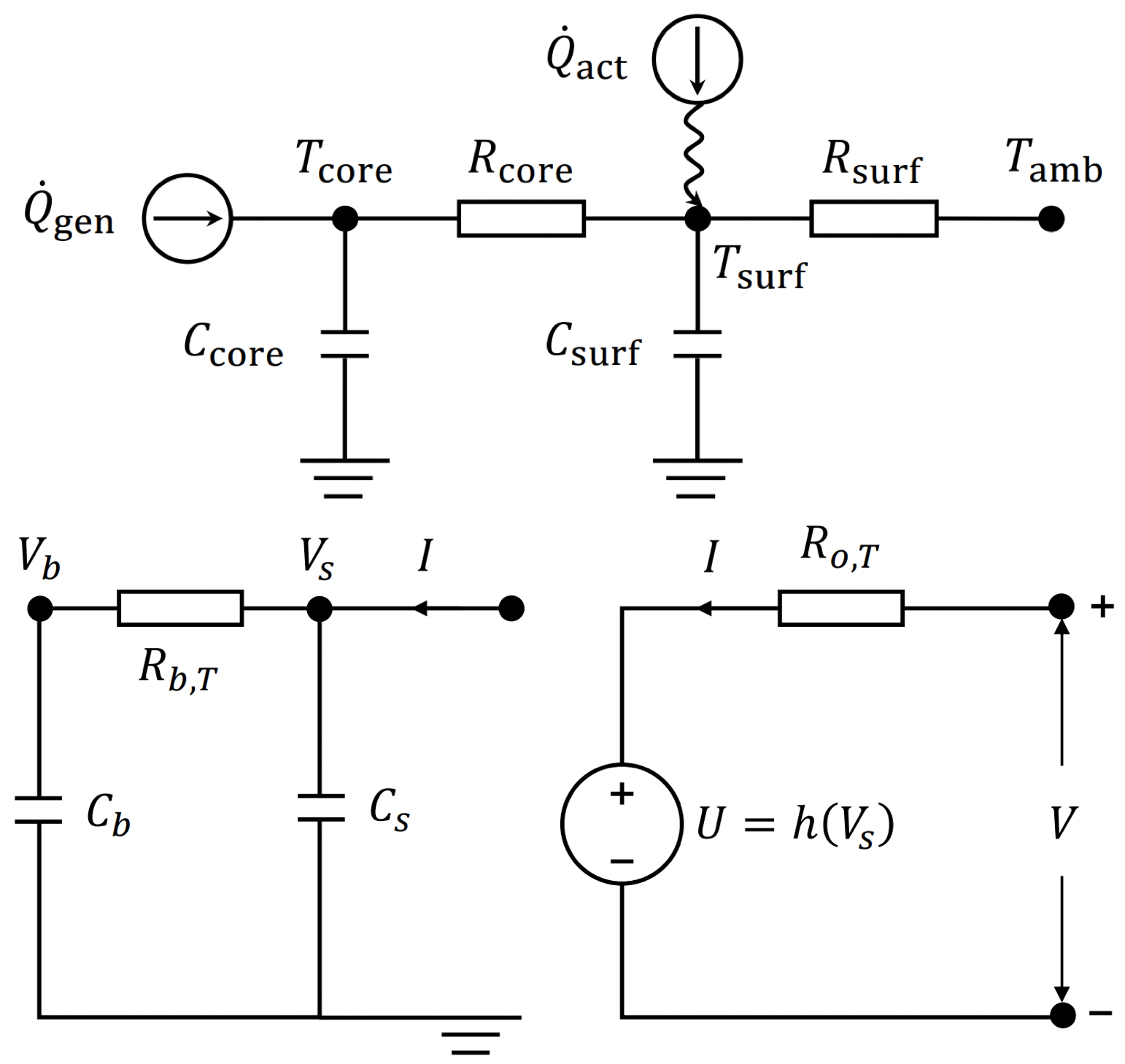
Figure 1: The thermal-NDC (nonlinear double-capacitor) model.

As shown in the lower portion of Fig. 1, the thermal-NDC model uses electrical circuits to describe the diffusion and electrical process inside a Lithium-ion battery (LiB) cell. It contains two coupled sub-circuits. The first (left) circuit contains two parallel connected capacitors, $C_{\mathrm{b}}$ and $C_{\mathrm{s}}$, and one resistor $R_{\mathrm{b,T}}$. The migration of charge between $C_{\mathrm{b}}$ and $C_{\mathrm{s}}$ mimics the change of Lithium-ion concentrations within the electrode. Conceptually, $C_{\mathrm{b}}$ and $C_{\mathrm{s}}$ represent the electrode’s bulk inner region and surface region, respectively. The second (right) circuit contains two components in series, a voltage source $U$ and a resistor $R_{\mathrm{o,T}}$. Here, $U=h(V_{\mathrm{s}})$ serves as an open-circuit voltage source. $R_{\mathrm{o,T}}$ corresponds to the ohmic resistance and solid electrolyte interface resistance. The first portion of the thermal-NDC model’s governing equations is summarized in the following state-space form:

$$\begin{bmatrix}\dot{V}_{\mathrm{b}}(t)\\ \dot{V}_{\mathrm{s}}(t)\end{bmatrix} =\boldsymbol{A}_{1}(t)\begin{bmatrix}V_{\mathrm{b}}(t)\\ V_{\mathrm{s}}(t)\end{bmatrix}+\boldsymbol{B}_{1}I(t),$$ (1a)

$$V(t) =h(V_{\mathrm{s}}(t))+R_{\mathrm{o,T}}(t)I(t),$$ (1b)

where $V_{\mathrm{b}}(t)$ and $V_{\mathrm{s}}(t)$ are the voltage across $C_{\mathrm{b}}$ and $C_{\mathrm{s}}$, respectively; $I(t)$ is the input current; $I(t)<0$ for discharging and $I(t)>0$ for charging; $h:\mathbb{R}\mapsto\mathbb{R}$ denotes a mapping from $V_{\mathrm{s}}(t)$ to the open circuit voltage source, which is determined by experiments; the matrices $A_{1}(t)$ and $B_{1}$ are given by

$$\boldsymbol{A}_{1}(t)=\begin{bmatrix}\dfrac{-1}{C_{\mathrm{b}}R_{\mathrm{b,T}}(t)}&\dfrac{1}{C_{\mathrm{b}}R_{\mathrm{b,T}}(t)}\\ \dfrac{1}{C_{\mathrm{s}}R_{\mathrm{b,T}}(t)}&\dfrac{-1}{C_{\mathrm{s}}R_{\mathrm{b,T}}(t)}\end{bmatrix},\ \boldsymbol{B}_{1}=\begin{bmatrix}0\\ \dfrac{1}{C_{\mathrm{s}}}\end{bmatrix}.$$ (2)

The state of charge (SoC) is given by:

$$\mathrm{SoC}(t)=(C_{\mathrm{b}}V_{\mathrm{b}}(t)+C_{\mathrm{s}}V_{\mathrm{s}}(t))/(C_{\mathrm{b}}+C_{\mathrm{s}})\times 100\%.$$ (3)

This paper aims to formulate a minimal state-space representation for the battery dynamics, thus SoC is not a state of the system but acts as another state coordinate of the states $V_{\mathrm{b}}$ and $V_{\mathrm{b}}$. In other words, according to (3), one can determine SoC by $V_{\mathrm{b}}$ and $V_{\mathrm{b}}$, and replace SoC by $(C_{\mathrm{b}}V_{\mathrm{b}}(t)+C_{\mathrm{s}}V_{\mathrm{s}}(t))/(C_{\mathrm{b}}+C_{\mathrm{s}})$. Here, $V_{\mathrm{b}}=V_{\mathrm{s}}=0$ V when the cell is depleted ($\mathrm{SoC}=0\%$), and $V_{\mathrm{b}}=V_{\mathrm{s}}=1$ V when the cell is fully charged ($\mathrm{SoC}=100\%$). The internal resistance $R_{\mathrm{o,T}}$ is assumed to be dependent on both temperature and SoC and is given by:

$$\begin{split}&R_{\mathrm{o,T}}(t)=R_{\mathrm{o}}(\mathrm{SoC}(t))\cdot\text{exp}(\kappa_{1}(\frac{1}{T_{\mathrm{core}}(t)}-\frac{1}{T_{\mathrm{ref}}})),\\ &R_{\mathrm{o}}(\mathrm{SoC}(t))=\gamma_{1}+\gamma_{2}\cdot\text{exp}(-\gamma_{3}\mathrm{SoC}(t)),\end{split}$$ (4)

where $\kappa_{1},\gamma_{1},\gamma_{2},\gamma_{3}\in\mathbb{R}$ are battery-dependent parameters and determined by experiments; $T_{\mathrm{core}}$ is the core temperature of the cell, which is later described in the lumped thermal model; $T_{\mathrm{ref}}$ is the reference temperature in the Arrhenius law. The diffusion resistance $R_{\mathrm{b,T}}$ is also temperature-dependent and given by:

$$R_{\mathrm{b,T}}(t)=R_{\mathrm{b}}\cdot\text{exp}(\kappa_{2}(\frac{1}{T_{\mathrm{core}}(t)}-\frac{1}{T_{\mathrm{ref}}})),$$ (5)

where $\kappa_{2}\in\mathbb{R}$ is a battery-dependent parameter and determined by experiments.

As shown in the upper portion of Fig. 1, a two-state lumped thermal model is used to capture the thermal dynamics of a cylindrical LiB cell. The temperature along the cell’s axial direction is assumed to be uniform. The cell’s temperature distribution along the radial direction is simplified to two singular points which represent the core and surface. The battery surface temperature is affected by $\dot{Q}_{\mathrm{act}}$ from active thermal input and the diffusion between the surface and the environment. The second portion of the thermal-NDC model’s governing equations is given by:

$$\begin{bmatrix}\dot{T}_{\mathrm{core}}(t)\\ \dot{T}_{\mathrm{surf}}(t)\end{bmatrix}=\boldsymbol{A}_{2}\begin{bmatrix}T_{\mathrm{core}}(t)\\ T_{\mathrm{surf}}(t)\end{bmatrix}+\boldsymbol{B}_{2}\begin{bmatrix}\dot{Q}_{\mathrm{gen}}(t)\\ T_{\mathrm{amb}}(t)\\ \dot{Q}_{\mathrm{act}}(t)\end{bmatrix},$$ (6)

where

$$\begin{split}\boldsymbol{A}_{2}&=\begin{bmatrix}\dfrac{-1}{R_{\mathrm{core}}C_{\mathrm{core}}}&\dfrac{1}{R_{\mathrm{core}}C_{\mathrm{core}}}\\ \dfrac{1}{R_{\mathrm{core}}C_{\mathrm{surf}}}&\dfrac{-1}{R_{\mathrm{surf}}C_{\mathrm{surf}}}+\dfrac{-1}{R_{\mathrm{core}}C_{\mathrm{surf}}}\end{bmatrix},\\ \boldsymbol{B}_{2}&=\begin{bmatrix}\dfrac{1}{C_{\mathrm{core}}}&0&0\\ 0&\dfrac{1}{R_{\mathrm{surf}}C_{\mathrm{surf}}}&\dfrac{1}{C_{\mathrm{surf}}}\end{bmatrix}.\end{split}$$

Here, $T_{\mathrm{core}}(t)$ and $T_{\mathrm{surf}}(t)$ are the temperature at the core and surface of the cell, respectively; $T_{\mathrm{amb}}(t)$ is the known ambient temperature at time $t$; $C_{\mathrm{core}}$ and $C_{\mathrm{surf}}$ are the cell’s core and surface heat capacity. A thermal resistance $R_{\mathrm{core}}$ is used to model the conduction between the cell’s core and surface. $R_{\mathrm{surf}}$ is the other thermal resistance that captures the convection between the cell’s surface and the environment. In addition, the heat generation inside the cell is assumed to be concentrated in the core of the cell, which is considered to be

$$\dot{Q}_{\mathrm{gen}}(t)=I(t)(V(t)-h(\mathrm{SoC}(t))).$$ (7)

The effect of the heating and cooling systems is reflected in the heat exchange between the hot/cold plates to the cell’s surface, i.e.

$$\dot{Q}_{\mathrm{act}}(t)=\eta_{\mathrm{act}}P_{\mathrm{act}}(t),$$ (8)

where $P_{\mathrm{act}}(t)>0$ and $P_{\mathrm{act}}(t)<0$ indicates the active heating and cooling power, respectively; $\eta_{\mathrm{act}}\in[0,1]$ is the efficiency coefficient.

Remark 1.

For simplicity, (8) assumes the same efficiency for heating and cooling. Nevertheless, one can directly convert (8) into heating and cooling power with different efficiency. In detail, (8) can be written as

$$\dot{Q}_{\mathrm{act}}(t)=P_{\mathrm{neat}}(t)\equiv\eta_{\mathrm{heat}}P_{\mathrm{heat}}(t)+\eta_{\mathrm{cool}}P_{\mathrm{cool}}(t),$$ (9)

where $P_{\mathrm{neat}}(t)$ is a decision variable. Let $P_{\mathrm{heat}}(t)\in[0,\overline{P}_{\mathrm{heat}}]$ and $P_{\mathrm{cool}}(t)\in[\underline{P}_{\mathrm{cool}},0]$. Then given the sign of $P_{\mathrm{neat}}(t)$, one can directly determine the value of $P_{\mathrm{heat}}(t)$ and $P_{\mathrm{cool}}(t)$. Given the power limit of $P_{\mathrm{heat}}(t)$ and $P_{\mathrm{cool}}(t)$, $P_{\mathrm{neat}}(t)\in[\eta_{\mathrm{cool}}\underline{P}_{\mathrm{cool}},\eta_{\mathrm{heat}}\overline{P}_{\mathrm{heat}}]$.

To summarize, given the thermal-NDC model, the state of the entire battery system at time instance $t$ is defined as

$$\boldsymbol{x}(t)\triangleq\begin{bmatrix}V_{\mathrm{b}}(t)&V_{\mathrm{s}}(t)&T_{\mathrm{core}}(t)&T_{\mathrm{surf}}(t)\end{bmatrix}^{\top}\in\mathbb{R}^{4}.$$

The input of the system at time instance $t$ is defined as

$$\boldsymbol{u}(t)\triangleq\begin{bmatrix}I(t)&P_{\mathrm{act}}(t)\end{bmatrix}^{\top}\in\mathbb{R}^{2}.$$

The output of the system at time instance $t$ is defined as

$$\boldsymbol{y}(t)\triangleq\begin{bmatrix}T_{\mathrm{surf}}(t)&V(t)\end{bmatrix}^{\top}\in\mathbb{R}^{2}.$$

The continuous-time system dynamics can be written as

$$\begin{split}\dot{\boldsymbol{x}}&=\boldsymbol{f}_{\mathrm{c}}(\boldsymbol{x},\boldsymbol{u}),\\ \boldsymbol{y}&=\boldsymbol{g}(\boldsymbol{x},\boldsymbol{u}),\end{split}$$ (10)

where the mapping $\boldsymbol{f}_{\mathrm{c}}:\mathbb{R}^{4}\times\mathbb{R}^{2}\mapsto\mathbb{R}^{4}$ and $\boldsymbol{g}:\mathbb{R}^{4}\times\mathbb{R}^{2}\mapsto\mathbb{R}^{2}$ are nonlinear and given by the combination of (1) - (8).

III Model Predictive Control Formulation

The problem of interest is to design a discrete-time control law for optimal charging while considering some safety and health constraints on LiBs, even if the ambient temperature is extremely high or low. This section formulates a battery charging problem with a discrete-time MPC strategy.

III-A Constraints

This subsection first introduces some constraints which ensure safe and health-conscious charging. To begin with, the SoC must be constrained to avoid overcharging, i.e.

$$\underline{\mathrm{SoC}}\leq\mathrm{SoC}(t)\leq\overline{\mathrm{SoC}},\ \forall t.$$ (11)

The current, terminal voltage and temperature must be within limits, i.e. $\forall t$,

$$\underline{I} \leq I(t)\leq\overline{I},$$ (12a)

$$\underline{V} \leq V(t)\leq\overline{V},$$ (12b)

$$\underline{T}_{\mathrm{core}} \leq T_{\mathrm{core}}(t)\leq\overline{T}_{\mathrm{core}}.$$ (12c)

In the thermal-NDC model, $V_{\mathrm{b}}$ and $V_{\mathrm{s}}$ serve as an analogy to the Li-ion concentrations at the bulk inner and surface region of the electrode, respectively. Hence, the $V_{\mathrm{b}}$ and $V_{\mathrm{s}}$ also need constraints, as suggested in [28]. Since $V_{\mathrm{b}}\leq V_{\mathrm{s}}$ during charging, one only needs to limit $V_{\mathrm{s}}$, i.e.

$$\underline{V}_{\mathrm{s}}\leq V_{\mathrm{s}}(t)\leq\overline{V}_{\mathrm{s}},\ \forall t.$$ (13)

$V_{\mathrm{s}}-V_{\mathrm{b}}$ indicates the Li-ion concentration gradient within the electrode, which is related to the battery’s capacity degradation and cycle life. The constraint is designed to be

$$V_{\mathrm{s}}(t)-V_{\mathrm{b}}(t)\leq\beta_{1}\mathrm{SoC}(t)+\beta_{2},\ \forall t,$$ (14)

where $\beta_{1},\beta_{2}\in\mathbb{R}$ are coefficients. Together with (3), this constraint can be rewritten as

$$\zeta(t)\leq\beta_{2},\ \forall t,$$ (15)

where $\zeta(t)\triangleq-\frac{C_{\mathrm{b}}+C_{\mathrm{s}}+\beta_{1}C_{\mathrm{b}}}{C_{\mathrm{b}}+C_{\mathrm{s}}}V_{\mathrm{b}}(t)+\frac{C_{\mathrm{b}}+C_{\mathrm{s}}-\beta_{1}C_{\mathrm{s}}}{C_{\mathrm{b}}+C_{\mathrm{s}}}V_{\mathrm{s}}(t)$. Finally, a constraint on the active battery temperature regulation system is considered, i.e.

$$\underline{P}_{\mathrm{act}}\leq P_{\mathrm{act}}(t)\leq\overline{P}_{\mathrm{act}},\ \forall t,$$ (16)

where $\underline{P}_{\mathrm{act}}$ and $\overline{P}_{\mathrm{act}}$ indicate the battery cooling and heating power limits, respectively.

III-B State-Feedback Model Predictive Control

This subsection introduces the formulation of a discrete-time state-feedback MPC for the battery charging problem. Let $N\in\mathbb{N}$ denote the number of steps in a prediction horizon and $\boldsymbol{x}_{k}\coloneqq\boldsymbol{x}(t_{k})$. By Euler integration with a planning time interval $\Delta_{\mathrm{p}}>0$, one obtains the following discretization of the continuous system in (10) for MPC:

$$\begin{split}\boldsymbol{x}_{k+1}&=\boldsymbol{x}_{k}+\Delta_{\mathrm{p}}\boldsymbol{f}_{\mathrm{c}}(\boldsymbol{x}_{k},\boldsymbol{u}_{k}),\\ \boldsymbol{y}_{k}&=\boldsymbol{g}(\boldsymbol{x}_{k},\boldsymbol{u}_{k}).\\ \end{split}$$ (17)

Denote $\boldsymbol{x}_{0:N|k}\triangleq\text{col}\{\boldsymbol{x}_{k},\boldsymbol{x}_{k+1|k}\cdots,\boldsymbol{x}_{k+N|k}\}\in\mathbb{R}^{4(N+1)}$ the state at time $t_{k}$ and the states from the future time $t_{k+1}$ to $t_{k+N}$ that are predicted at time $t_{k}$; similarly $\boldsymbol{u}_{0:N-1|k}\triangleq\text{col}\{\boldsymbol{u}_{k|k},\cdots,\boldsymbol{u}_{k+N-1|k}\}\in\mathbb{R}^{2N}$; particularly denote $\mathrm{SoC}_{0:N|k}\triangleq\text{col}\{\mathrm{SoC}_{k|k},\cdots,\mathrm{SoC}_{k+N|k}\}\in\mathbb{R}^{N+1}$ and $V_{0:N-1|k}\triangleq\text{col}\{V_{k|k},\cdots,V_{k+N-1|k}\}\in\mathbb{R}^{N}$. Define the objective function $J\coloneqq J(\boldsymbol{x}_{0:N|k},\boldsymbol{u}_{0:N-1|k})$ as

$$\begin{split}J\triangleq&w_{1}\textstyle\sum_{j=0}^{N}(\mathrm{SoC}_{k+j|k}-\mathrm{SoC}_{\mathrm{r}})^{2}+\\ &w_{2}\textstyle\sum_{j=0}^{N-2}(I_{k+j+1|k}-I_{k+j|k})^{2}+\\ &w_{3}\textstyle\sum_{j=0}^{N-2}(P_{\mathrm{act},k+j+1|k}-P_{\mathrm{act},k+j|k})^{2},\end{split}$$ (18)

where $\mathrm{SoC}_{\mathrm{r}}$ is the target SoC to be charged, $w_{1},w_{2},w_{3}>0$ are some weights. The first term of this objective function reflects that the battery is desired to be charged as soon as possible. The second and third terms encourage the current’s and thermal power’s smoothness over time, respectively.

Remark 2.

Depending on the specific configuration of the battery cooling and heating system and their actuators, the definition of $P_{\mathrm{act}}$’s smoothness could be different. This paper adopts the general form to define smoothness since modeling the actuators is not within this paper’s scope.

Then at time $t_{k}$, given the state $\boldsymbol{x}_{k}$ and the ambient temperature $T_{\mathrm{amb},k}\coloneqq T_{\mathrm{amb}}(t_{k})$, assuming that $T_{\mathrm{amb},k+j|k}\equiv T_{\mathrm{amb},k},\ \forall j\in\llbracket 0,N\rrbracket$, the optimal control can be determined by —s— u_0:N-1—k J(x_0:N—k,u_0:N-1—k) x_k+j+1—k = x_k+j—k + Δ_p f_c(x_k+j—k, u_k+j—k) y_k+j—k= g(x_k+j—k,u_k+j—k) ∀j ∈⟦0,N-1 ⟧  with given x_k constraints (11), (12c)-(16),  ∀j ∈⟦0,N ⟧ constraints (12a), (12b),  ∀j ∈⟦0,N-1 ⟧.

The state-feedback MPC algorithm is summarized in Algorithm 1. As shown by Line 2, the system state is observed with a smaller sampling time $\Delta_{\mathrm{s}}$, i.e. $\Delta_{\mathrm{s}}<\Delta_{\mathrm{p}}$. The MPC is computed for every time interval $\Delta_{\mathrm{p}}$ given the present state $\boldsymbol{x}_{k}$ at time $t_{k}$, as shown by Line 3. Then for every time instance $t_{i}$, the input $\boldsymbol{u}_{i}$ is calculated by interpolating the optimal control trajectory from the MPC with zero-order hold, as indicated in Line 8.

Input: $k=-1$, $i=0$, $t_{0}=0$, $\Delta_{\mathrm{p}}$, $\Delta_{\mathrm{s}}$

1 while $\mathrm{SoC}_{i}<\mathrm{SoC}_{\mathrm{r}}$ do

2       observe $\boldsymbol{x}_{i}$ and $T_{\mathrm{amb},i}$ at time $t_{i}$

3      

4      if $t_{i}\ \%\ \Delta_{\mathrm{p}}==0$ then // for every time interval $\Delta_{\mathrm{p}}$

5             $k\leftarrow k+1$

6             $\boldsymbol{u}^{*}_{0:N-1|k}\leftarrow$ solve $\eqref{eq:oc_mpc_1}$ given $\boldsymbol{x}_{k}$ at time $t_{k}$ and $T_{\mathrm{amb},k+j|k}\equiv T_{\mathrm{amb},k},\ \forall j\in\llbracket 0,N\rrbracket$

7             $t_{k}\leftarrow t_{k}+\Delta_{\mathrm{p}}$

8       else

9             perform $\boldsymbol{u}_{i}$ by interpolating $\boldsymbol{u}^{*}_{0:N-1|k}$ with present time $t_{i}$ and zero-order hold

10            

11      $t_{i}\leftarrow t_{i}+\Delta_{\mathrm{s}}$, $i\leftarrow i+1$

12      

Algorithm 1 State-Feedback MPC

III-C System Parameters

The necessary parameters for the battery dynamics (10) and the constraints (11) - (16) are given by Table I. The system parameters are given in [12], using a 3 Ah Panasonic NCR-18650B LiB battery. The constraint parameters are derived from [28]. $\overline{P}_{\mathrm{heat}}$ and $\overline{P}_{\mathrm{cool}}$ are determined by scaling the power limits in [31]. The mapping $h(\cdot)$ in (1b) is parameterized by a fifth-order polynomial [12], i.e.

$$h(V_{\mathrm{s}})=\textstyle\sum_{i=0}^{5}\alpha_{i}V_{\mathrm{s}}^{i}.$$ (19)

The model parameters are validated for charging current up to 4.5 A, whose maximum charging C-rate is 1.5 C. This paper defines the upper bound for charging current as $\overline{I}=3$ A. Note that the unit for all the temperature variables or bounds is Kelvin. But for the sake of readability, the rest of this paper adopts degree Celsius to express the same temperature in Kelvin.

Table I: Battery Parameters

Parameter	Value	Param.	Value	Param.	Value
$C_{\mathrm{b}}$	10037 F	$C_{\mathrm{core}}$	40 F	$\underline{\mathrm{SoC}}$	0%
$C_{\mathrm{s}}$	973 F	$C_{\mathrm{surf}}$	10 F	$\overline{\mathrm{SoC}}$	100%
$R_{\mathrm{b}}$	0.019 $\Omega$	$R_{\mathrm{core}}$	4 $\Omega$	$\underline{I}$	0 A
$\gamma_{1}$	0.026	$R_{\mathrm{surf}}$	7 $\Omega$	$\overline{I}$	3 A
$\gamma_{2}$	0.061	$\kappa_{1}$	30	$\underline{V}$	0 V
$\gamma_{3}$	14.36	$\kappa_{2}$	70	$\overline{V}$	4.2 V
$\alpha_{0}$	3.2	$T_{\mathrm{ref}}$	25 ∘C	$\underline{T}_{\mathrm{core}}$	-10 ∘C
$\alpha_{1}$	2.59	$\eta_{\mathrm{act}}$	87%	$\overline{T}_{\mathrm{core}}$	55 ∘C
$\alpha_{2}$	-9.003	$\beta_{1}$	-0.04	$\underline{V}_{\mathrm{b}}$	0 V
$\alpha_{3}$	18.87	$\beta_{2}$	0.08	$\overline{V}_{\mathrm{b}}$	0.95 V
$\alpha_{4}$	-17.82	$\underline{P}_{\mathrm{act}}$	-8 W	$\underline{V}_{\mathrm{s}}$	0 V
$\alpha_{5}$	6.325	$\overline{P}_{\mathrm{act}}$	8 W	$\overline{V}_{\mathrm{s}}$	0.95 V

IV Numerical Experiments

This section presents several case studies with numerical experiments to illustrate the effectiveness of the proposed thermal-NDC model in integrated charging and active thermal management under extreme ambient temperatures. Additionally, this section investigates the impact of MPC parameters, battery core temperature, and active thermal power on fast charging. Several insights are revealed and summarized in this section to explain why the decisions made by the proposed algorithm lead to energy-efficient fast charging.

IV-A Basic Case Study

With the proposed thermal-NDC model, this subsection performs several case studies with low, mild, and high ambient temperatures and compares the battery charging performance with several strategies to verify the effectiveness of the proposed charging strategies. The list of all strategies is summarized in Table II. Strategy B adopts the same MPC scheme (2) without active thermal management involved in the MPC formulation to mimic the existing battery modeling without external thermal influence. B utilizes a separate PID temperature controller, which is common in industry, i.e.

$$\begin{split}e(t_{k})&\coloneqq e_{k}=T_{\mathrm{core,r}}-T_{\mathrm{core},k},\\ P_{\mathrm{act},k}&=[K_{\mathrm{P}}e_{k}+K_{\mathrm{I}}\textstyle\sum_{j=0}^{k}e_{j}+K_{\mathrm{D}}\dot{e}(t_{k})]_{\underline{P}_{\mathrm{act}}}^{\overline{P}_{\mathrm{act}}},\\ \end{split}$$ (20)

where $T_{\mathrm{core,r}}$ is the desired battery core temperature; $T_{\mathrm{core,k}}$ is the battery core temperature at time $t_{k}$; $K_{\mathrm{P}},K_{\mathrm{I}},K_{\mathrm{D}}\geq 0$ are the proportional, integral, and derivative gain, respectively; $[\cdot]_{\underline{P}_{\mathrm{act}}}^{\overline{P}_{\mathrm{act}}}$ denotes the clip function with maximum value $\overline{P}_{\mathrm{act}}$ and minimum value $\underline{P}_{\mathrm{act}}$; $\dot{e}(t_{k})\coloneqq-\dot{T}_{\mathrm{core}}(t_{k})$, and $\dot{T}_{\mathrm{core}}(t_{k})$ is estimated by applying the optimal control $\boldsymbol{u}^{*}_{k|k}$ at time $t_{k}$ without active thermal control to the system dynamics (6).

Table II: Strategy Description for Basic Case Study

Name	Description
P	the proposed MPC (2), optimization initial guess given by forward propagating dynamics with zero inputs
P1	same as P, optimization initial guess given by forward propagating dynamics with maximum charging current and $P_{\mathrm{act},k}$; $P_{\mathrm{act},k}$ is forwardly calculated by (20) with $T_{\mathrm{core,r}}=45$ ${}^{\circ}\text{C}$
A	the proposed MPC (2) without active thermal management, i.e. $\underline{P}_{\mathrm{act}}=\overline{P}_{\mathrm{act}}=0$ W, $P_{\mathrm{act}}(t)=0,\ \forall t$
B	A, battery temperature is separately controlled by the PID controller (20), $T_{\mathrm{core,r}}=25$ ${}^{\circ}\text{C}$
C	same as B, $T_{\mathrm{core,r}}=35$ ${}^{\circ}\text{C}$
D	same as B, $T_{\mathrm{core,r}}=45$ ${}^{\circ}\text{C}$
E	same as B, $T_{\mathrm{core,r}}=50$ ${}^{\circ}\text{C}$

The parameters used in the basic case study are: $\mathrm{SoC_{r}}=0.90$, $w_{1}=40$, $w_{2}=0.1$, $w_{3}=0.1$, $\Delta_{\mathrm{p}}=5$ s, $\Delta_{\mathrm{s}}=1$ s, $N=40$, $K_{\mathrm{P}}=0.5$, $K_{\mathrm{I}}=0.01$, $K_{\mathrm{P}}=150$. The discrete-time system dynamics in the simulation is updated in every time interval $\Delta_{\mathrm{s}}$ and given by

$$\boldsymbol{x}_{i+1}=\boldsymbol{x}_{i}+\Delta_{\mathrm{s}}\boldsymbol{f}_{\mathrm{c}}(\boldsymbol{x}_{i},\boldsymbol{u}_{i}).$$ (21)

The PID gains are tuned appropriately to minimize the rising time, overshoot, and steady-state error on temperature tracking. When strategies involve solving the optimal control instance (2), the optimal control instance is programmed by Python with CasADi [32], compiled as a C library with a nonlinear programming solver IPOPT [33] with MUMPS, and then executed at run-time in Python. All the simulations are run on a 2017 MacBook Pro equipped with a 3.1-GHz Inter Core i7 and 16 GB RAM.

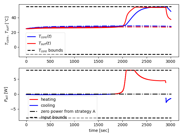
(a) Result by P and A with $T_{\mathrm{amb}}=25$ ${}^{\circ}\text{C}$.

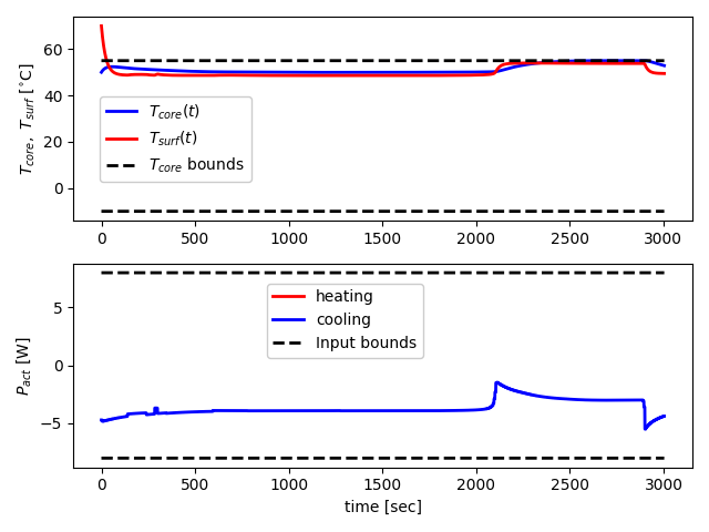
(b) Result by P with $T_{\mathrm{amb}}=70$ ${}^{\circ}\text{C}$.

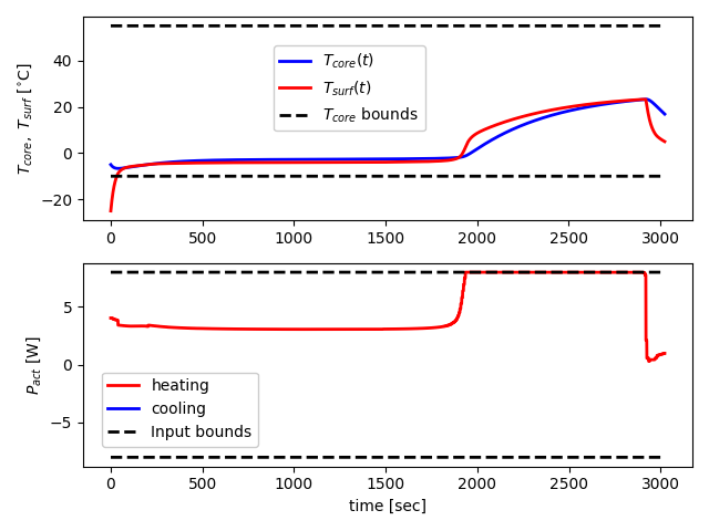
(c) Result by P with $T_{\mathrm{amb}}=-25$ ${}^{\circ}\text{C}$.

Figure 2: Battery core and surface temperature and active thermal power by some strategies in different ambient temperatures. In the upper portion of each subfigure, the solid lines in blue and red represent $T_{\mathrm{core}}$ and $T_{\mathrm{surf}}$ by strategy P. In the lower portion of each subfigure, the solid lines in blue and red represent the active cooling and heating power by P. In subfigure (a), the dash-dot lines in blue and red represent $T_{\mathrm{core}}$ and $T_{\mathrm{surf}}$ by strategy A; the dash-dot line in black represents the zero active thermal power by A. Note that there is no constraint on $T_{\mathrm{surf}}$.

IV-A1 Mild Ambient Temperature

The ambient temperature $T_{\mathrm{amb}}=25$ ${}^{\circ}\text{C}$. The initial state $\boldsymbol{x}_{0}=\begin{bmatrix}0.1\text{ V}&0.1\text{ V}&25\,^{\circ}\text{C}&25\,^{\circ}\text{C}\end{bmatrix}^{\top}$. The simulation results are shown in Table III, where $T_{\mathrm{chg}}$ indicates the total charging time; $T_{\mathrm{comp}}$ indicates the average computational time and its standard deviation; Energy indicates the total energy used for charging and thermal management; Efficiency indicates the charging efficiency (the ratio of the energy used for raising SoC to the total energy), i.e.

$$\frac{\sum_{k=0}^{T_{\mathrm{chg}}/\Delta_{\mathrm{s}}}I_{k}\cdot h(\mathrm{SoC}_{k})\Delta_{\mathrm{s}}}{\sum_{k=0}^{T_{\mathrm{chg}}/\Delta_{\mathrm{s}}}(I_{k}V_{k}+|P_{\mathrm{act},k}|)\Delta_{\mathrm{s}}}.$$

According to Table III, strategies P and P1 have the smallest charging time. As for total consumed energy and efficiency, A outperforms the others since charging the battery without active thermal management will not violate the battery temperature constraint when the ambient temperature is mild. Fig. 2a illustrates the trajectories of battery core and surface temperature and active thermal power for strategies P and A, where strategy P chooses to warm the battery after about 1800 s and thus results in faster charging. From strategies B to D, as the desired battery core temperature $T_{\mathrm{core,r}}$ increasing from 25 ${}^{\circ}\text{C}$ to 45 ${}^{\circ}\text{C}$, the charging time decreases from 3019 s to 3009 s. But when the desired core temperature $T_{\mathrm{core,r}}=50$ ${}^{\circ}\text{C}$ is closed to the upper bound $\overline{T}_{\mathrm{core}}=55$ ^∘C, the PID controller violates $\overline{T}_{\mathrm{core}}$ at 690 s - 1090 s since it has no predictive information on how the system dynamics will evolve. These observations are consistent with the statement that heating the battery could benefit the charging speed [6, 7].

Table III: Battery Charging Result in Mild Ambient Temperature

Strategy	$T_{\mathrm{chg}}$ [s]	Energy [kJ]	Efficiency	$T_{\mathrm{comp}}$ [ms]
P	3005	38.98	83.10%	$23.59\pm 4.38$
P1	3005	38.99	83.08%	$21.66\pm 4.99$
A	3017	33.42	96.93%	$22.14\pm 3.67$
B	3019	35.25	91.90%	$21.47\pm 2.16$
C	3013	37.24	86.98%	$21.90\pm 2.36$
D	3009	42.88	75.54%	$21.53\pm 2.38$
E†	3416	47.39	68.35%	$23.40\pm 6.58$

• Infeasible at 690 - 1090 s; violates $\overline{T}_{\mathrm{core}}$

IV-A2 High Ambient Temperature

The ambient temperature $T_{\mathrm{amb}}=70$ ${}^{\circ}\text{C}$. The initial state $\boldsymbol{x}_{0}=\begin{bmatrix}0.1\text{ V}&0.1\text{ V}&50\,^{\circ}\text{C}&70\,^{\circ}\text{C}\end{bmatrix}^{\top}$. Note that this initial state is more challenging than $T_{\mathrm{core}}=T_{\mathrm{surf}}=50$ ${}^{\circ}\text{C}$ since the heat convection from the surface to the core could further increase the core temperature. The simulation results are shown in Table IV, where strategies P and P1 have the smallest charging time but have slightly different total consumed energy and efficiency. A conjecture is that the real difference in charging time could be less than the time resolution of the simulation $\Delta_{\mathrm{s}}=1$ s; the slightly different control trajectories lead to different values on the accumulated energy consumption and efficiency. Strategies A - E cannot find a feasible solution for solving MPC instances over some duration when the ambient temperature is high, which reflects that these strategies are not applicable at run-time in this scenario. A practical workaround for these strategies is to solely adjust the battery temperature to a mild range first, then charge the battery. This solution leads to longer charging time because it cannot jointly determine the battery’s electrical and thermal control. This case study verifies the effectiveness of the proposed strategies P and P1 with high ambient temperature. Fig. 2b illustrates the trajectories of battery temperature and active thermal power for strategy P, where the active cooling power is regulated to balance the heat convention among the ambient, the battery surface, and the battery core.

Table IV: Battery Charging Result in High Ambient Temperature

Strategy	$T_{\mathrm{chg}}$ [s]	Energy [kJ]	Efficiency	$T_{\mathrm{comp}}$ [ms]
P	3004	44.43	72.91%	$25.45\pm 4.85$
P1	3004	44.45	72.87%	$20.88\pm 4.99$
A†	N/A	N/A	N/A	$49.76\pm 4.28$
B‡	3098	58.20	55.65%	$21.52\pm 4.17$
C∗	3131	55.24	59.72%	$21.70\pm 5.00$
D∗∗	3416	49.55	65.37%	$23.74\pm 7.76$
E†	N/A	N/A	N/A	$42.04\pm 2.96$

• Infeasible until simulation timeouts

• Infeasible in the first 70 s

• Infeasible in the first 105 s

• Infeasible in the first 385 s

IV-A3 Low Ambient Temperature

The ambient temperature $T_{\mathrm{amb}}=-25$ ${}^{\circ}\text{C}$. The initial state $\boldsymbol{x}_{0}=\begin{bmatrix}0.1\text{ V}&0.1\text{ V}&-5\,^{\circ}\text{C}&-25\,^{\circ}\text{C}\end{bmatrix}^{\top}$. The simulation results are shown in Table V. Considering the constraint satisfaction and the MPC solution feasibility, strategy P outperforms the others in charging time, total energy consumption, and efficiency. Strategy P1 has the same charging time as P but the energy consumption and efficiency are slightly different than P1’s due to the same reason mentioned in Section IV-A2. Strategies A - E cannot find a feasible solution for solving MPC instances over some duration since the battery temperature is close to the lower bound. Since the constraints on $T_{\mathrm{core}}$, $V$, and $\zeta$ limit the charging speed and strategies B - E violate some of them, their total charging time are less than P’s and P1’s. Violating these constraints during fast charging could jeopardize the battery health [28]. Thus, these strategies are not applicable at run-time when the ambient temperature is low. Fig. 2c illustrates the trajectories of battery temperature and active thermal power for strategy P, where the active heating power hits the upper bound to warm up the battery for fast charging.

Table V: Battery Charging Result in Low Ambient Temperature

Strategy	$T_{\mathrm{chg}}$ [s]	Energy [kJ]	Efficiency	$T_{\mathrm{comp}}$ [ms]
P	3023	47.63	68.01%	$24.67\pm 4.85$
P1	3023	47.71	67.89%	$21.91\pm 5.45$
A†	N/A	N/A	N/A	$106.88\pm 63.50$
B‡	3022	57.60	56.24%	$21.93\pm 9.20$
C‡§	3022	57.60	56.24%	$21.96\pm 9.05$
D‡§	3023	47.63	68.01%	$24.67\pm 4.85$
E‡§	3022	57.60	56.24%	$21.98\pm 9.07$

• Infeasible until simulation timeouts

• Infeasible in the first 25 s

• Unable to reach $T_{\mathrm{core,r}}$ due to power limits

IV-A4 Summary on Basic Case Study

To summarize the three basic case studies above, the proposed strategies P and P1 outperform the others in charging time given three different ambient temperatures, which cover most of the battery operational conditions. Strategies A - E are not applicable at run-time when the ambient temperature is extreme since they might not find a feasible solution. Strategy P and P1 outperform the others in energy consumption and efficiency with both high and low ambient temperature even though these factors are not explicitly considered in the objective function. This is because, with the proposed thermal-NDC model, P and P1 can jointly determine control such that the battery temperature and SOC can be mutually beneficial to each other. To further improve energy efficiency and reduce energy consumption with mild ambient temperature, one could restrict the power limit on $P_{\mathrm{act}}$ given a certain range of mild ambient temperature.

The advantage of the proposed thermal-NDC model can be also reflected by an observation from Fig. 2, where $P_{\mathrm{act}}$ drops toward cooling to reduce $T_{\mathrm{core}}$ and $T_{\mathrm{surf}}$ at the end of charging. In fact, as Fig. 3 illustrated, the charging current also drops at the same time. The dropping on both $P_{\mathrm{act}}$ and $I$ is to reduce $V_{\mathrm{s}}$ and $V$ such that they will not violate the constraints as they approach the upper bounds closely. Also, as SOC increases, the upper bound on the Li-ion concentration gradient within the electrode, i.e. $\beta_{1}\mathrm{SoC}(t)+\beta_{2}$, decreases. This again requires $V_{\mathrm{s}}$ to reduce such that $V_{\mathrm{s}}-V_{\mathrm{b}}$ will not violate its upper bound. The system behaviors with $T_{\mathrm{amb}}=-25$ ${}^{\circ}\text{C}$ and $T_{\mathrm{amb}}=25$ ${}^{\circ}\text{C}$ are similar to Fig. 3, thereby omitted.

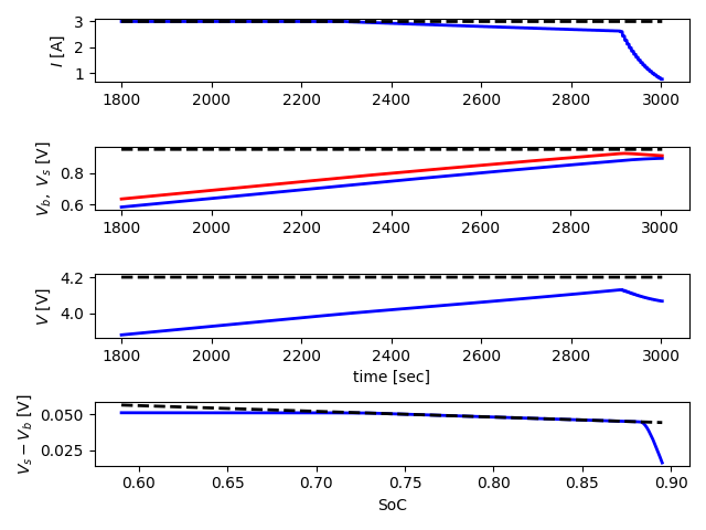
Figure 3: A trajectory segment for $I$, $V_{\mathrm{b}}$, $V_{\mathrm{s}}$, $V$, and $V_{\mathrm{s}}(t)-V_{\mathrm{b}}(t)$ vs $\beta_{1}\mathrm{SoC}(t)+\beta_{2}$ with $T_{\mathrm{amb}}=70$ ${}^{\circ}\text{C}$. The red and blue curves in the second subfigure indicate $V_{\mathrm{s}}$ and $V_{\mathrm{b}}$, respectively. The black dashed lines in the top three subfigures are the upper bounds. The black dashed line in the last subfigure indicates $\beta_{1}\mathrm{SoC}(t)+\beta_{2}$ as $\mathrm{SoC}(t)$ increases over time.

As for the computational time between P and P1, Tukey’s HSD (honestly significant difference) Test [34, Chapter 14] is performed for three cases and it reveals a statistically significant difference between the computational time of strategies P and P1; the computational time of P is statistically greater than P1’s with the p-value 0.00 $<$ 0.05. This indicates that the initial guess of P1’s MPC problem, i.e. regulating $T_{\mathrm{core}}$ to $T_{\mathrm{core,r}}=45$ ${}^{\circ}\text{C}$ in all three ambient temperatures, is closer to the optimum than P’s initial guess, which benefits the run-time computation.

A similar conclusion can be drawn based on the observation from Fig. 2, where the MPC strategy P seems to maintain a high $T_{\mathrm{core}}$ for fast charging. These two observations are consistent with the conclusions made by [6, 7]. However, compared with the results in mild and high ambient temperatures, it is uncertain that raising the heating power bound could further speed up the charging given low ambient temperature. Also, comparing the computational time of P and P1 in the low and high ambient temperatures, the initialization of P1, i.e. regulating $T_{\mathrm{core}}$ to $T_{\mathrm{core,r}}=45$ ${}^{\circ}\text{C}$, might be closer to the optimal solution than strategy P’s initialization. Thus, the next subsection investigates how battery core temperature and active heating would affect the charging speed, and verify whether an MPC strategy with a long enough horizon can obtain an optimal solution that implicitly encourages warming up the battery to an optimal temperature.

IV-B Other Factors

According to [6], the Lithium-ion battery temperature plays a significant role during charging and discharging, especially when the ambient temperature is below 0 ${}^{\circ}\text{C}$. Heating Lithium-ion batteries at the beginning of charging could improve the charging speed and capacity retention even if the ambient temperature is -30 ${}^{\circ}\text{C}$ [6, 7]. Therefore, with the proposed thermal-NDC model, this subsection performs several numerical experiments in low ambient temperatures to investigate how the MPC horizon and battery temperature affect the charging speed.

To investigate how $T_{\mathrm{core}}$ affects the charging speed, a revised objective function is given to explicitly warm up the battery core to a desired temperature while charging, i.e.

$$\begin{split}J_{2}\triangleq&w_{1}\textstyle\sum_{j=0}^{N}(\mathrm{SoC}_{k+j|k}-\mathrm{SoC}_{\mathrm{r}})^{2}+\\ &w_{2}\textstyle\sum_{j=0}^{N-2}(I_{k+j+1|k}-I_{k+j|k})^{2}+\\ &w_{3}\textstyle\sum_{j=0}^{N-2}(P_{\mathrm{act},k+j+1|k}-P_{\mathrm{act},k+j|k})^{2}+\\ &w_{4}\textstyle\sum_{j=0}^{N}(T_{\mathrm{core},k+j|k}-T_{\mathrm{core,r}})^{2},\end{split}$$ (22)

where $T_{\mathrm{core,r}}$ is a prescribed target battery core temperature, $w_{1},w_{2},w_{3},w_{4}>0$ are some weights. In this subsection, parameters are the same as the ones in Section IV-A, except for explicit annotations. $w_{4}=0.5$ when applicable. The power limits of $P_{\mathrm{act}}$ are relaxed as $[-24\text{ W},24\text{ W}]$ such that the system has enough power to regulate $T_{\mathrm{core}}$ within the range [-10 ^∘C, 55 ^∘C], in low ambient temperature. Table VI summarizes the additional strategies to be compared. The comparison results are summarized in Table VII.

Table VI: Strategy Description for Other Factors

Name	Description
P2	same as P†, objective function using $J_{2}$ in (22), $T_{\mathrm{core,r}}=45^{\circ}\text{C}$
P3	same as P2, $N=40$, $T_{\mathrm{core,r}}=55$ ${}^{\circ}\text{C}$
P4	same as P, $N=80$
P5	same as P, $N=120$

• Note: for strategy P, $N=40$

Regarding the computational time of the proposed strategies P and P1 - P5, a one-way analysis of variance (one-way ANOVA) [34, Chapter 14] is performed, which reveals a statistically significant difference in computational time between at least two groups with a p-value of $0.00<0.05$. Then Tukey’s HSD Test reveals a relation with statistical significance among these groups, i.e. P1 $<$ P $<$ P2 $<$ P3 $<$ P4 $<$ P5.

Table VII: Battery Charging Result in Low Ambient Temperature with Higher Heating/Cooling Power Limits

Strategy	$T_{\mathrm{chg}}$ [s]	Energy [kJ]	Efficiency	$T_{\mathrm{comp}}$ [ms]
P	3005	59.68	54.28%	$23.50\pm 4.39$
P1	3005	59.71	54.24%	$20.99\pm 4.86$
P2	3007	69.40	46.67%	$29.53\pm 29.00$
P3	3002	74.62	43.41%	$38.06\pm 27.85$
P4	3004	61.51	52.66%	$44.51\pm 9.46$
P5	3004	62.85	51.54%	$65.98\pm 13.04$
A†	N/A	N/A	N/A	$106.73\pm 63.01$
B‡	3024	58.48	55.39%	$21.47\pm 7.57$
C‡	3019	64.10	50.53%	$21.47\pm 7.52$
D§	3388	74.04	43.75%	$23.46\pm 9.14$
E∗	3846	82.82	39.11%	$27.90\pm 14.21$

• Infeasible until simulation timeouts

• Infeasible at 0 - 5 s

• Infeasible at 0 - 5 s, 755 - 1125 s; violates $\overline{T}_{\mathrm{core}}$

• Infeasible at 0 - 5 s, 600 - 1430 s; violates $\overline{T}_{\mathrm{core}}$

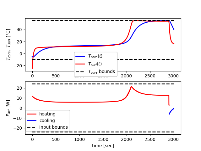
(a) Result by P1 with $T_{\mathrm{amb}}=-25$ ${}^{\circ}\text{C}$.

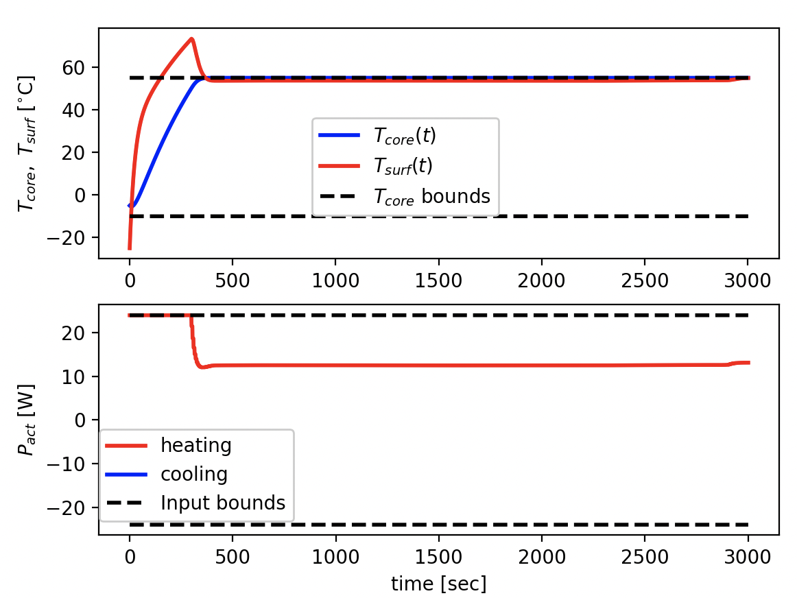
(b) Result by P3 with $T_{\mathrm{amb}}=-25$ ${}^{\circ}\text{C}$.

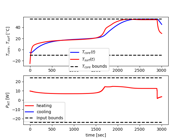
(c) Result by P5 with $T_{\mathrm{amb}}=-25$ ${}^{\circ}\text{C}$.

Figure 4: Battery core and surface temperature and active thermal power by strategies P1, P3, and P5 with larger thermal power bounds in the low ambient temperature. Note that there is no constraint on $T_{\mathrm{surf}}$.

As for the effect of $T_{\mathrm{core}}$ on charging speed, P3 outperforms the other strategies in terms of charging time. Meanwhile, the other proposed strategies yield slightly longer charging times. Nevertheless, P1 can achieve a good balance across all indices. Fig. 4b illustrates the reason why P3 outperforms the others on charging time, where P3 tracks $T_{\mathrm{core,r}}=55$ ${}^{\circ}\text{C}$ to maintain a high $T_{\mathrm{core}}$ for a longer duration than P1 and P5. The reason can be revealed by the proposed thermal-NDC model, where a higher $T_{\mathrm{core}}$ reduces the internal resistance $R_{\mathrm{b,T}}(t)$ as (5) describes, and further affects the capacitor voltage dynamics (1a). Since $\mathrm{SoC}(t)$ is defined as a linear combination of the capacitor voltages $V_{\mathrm{b}}(t)$ and $V_{\mathrm{s}}(t)$ in (3), the time derivative of SOC is directly affected by the capacitor voltage dynamics (1a). This explanation is consistent with the observation from numerical experiments, as well as the conclusions from the literature [6, 7]. However, heating the battery at the beginning as P3 does is not energy-efficient. Fig. 4a and Fig. 4c indicate that after the battery is charged for about 2200 s and 1700 s, P1 and P5 begin to heat the battery because they generate more heat by (7) with a higher $V$.

Comparing the results from Table VII and Fig. 4, P1 only increases the heating power after $\sim$2100 seconds, where the SOC is $\sim$65%. From the comparison of the MPC horizon $N$ in this subsection, the horizon of P (or P1) is long enough such that the MPC can obtain a solution that is at least close to the optimal one. Thus, explicitly regulating $T_{\mathrm{core}}$ as P2 and P3 do is not necessary. From the perspective of balancing the charging time and energy consumption, P1 performs better than the other strategies.

V EKF-Based Output-Feedback Model Predictive Control

The previous section studies the MPC of battery charging based on the assumption that the states are fully measurable. This assumption might not hold in real-world applications. Hence, this section proposes an output-feedback MPC based on Extended Kalman Filter (EKF) [35, Chapter 8.2]. The EKF takes in system output measurements and generates state estimates, which are given to a revised MPC controller to design control. This section presents a way to rewrite the proposed thermal-NDC model for the ease of EKF, proposes an EKF-based output-feedback MPC, and demonstrates the effectiveness of this algorithm under extreme ambient temperatures by numerical simulations.

V-A System Reformulation & Proposed Algorithm

The output $V$ is a function of both states and inputs, as shown in (1b), thus EKF is not applicable for this output form. This subsection first rewrites the original system dynamics (10) similarly as [28] such that its output is a function of states. To reformulate the system dynamics, new state, control, and output for the continuous-time system dynamics are defined as follows,

$$\begin{split}&\boldsymbol{x}(t)\triangleq\text{col}\{V_{\mathrm{b}},V_{\mathrm{s}},T_{\mathrm{core}},T_{\mathrm{surf}},I\}\in\mathbb{R}^{5},\\ &\boldsymbol{u}(t)\triangleq\text{col}\{u_{1},P_{\mathrm{act}}\}\in\mathbb{R}^{2},\\ &\boldsymbol{y}(t)\triangleq\text{col}\{T_{\mathrm{surf}},V,I\}\in\mathbb{R}^{3},\end{split}$$ (23)

where $u_{1}\in\mathbb{R}$ is a new control input such that the charging current has the following dynamics:

$$\dot{I}(t)=u_{1}(t).$$ (24)

Note that $\boldsymbol{y}(t)$ is measurable in practice.

Combining the previous dynamics (1) - (8) with the current dynamics (24), one obtains the following dynamics in continuous-time:

$$\dot{\boldsymbol{x}} =\hat{\boldsymbol{f}}_{\mathrm{c}}(\boldsymbol{x},\boldsymbol{u}),$$ (25a)

$$\boldsymbol{y} =\boldsymbol{h}(\boldsymbol{x}),$$ (25b)

where $\hat{\boldsymbol{f}}_{\mathrm{c}}:\mathbb{R}^{5}\times\mathbb{R}^{2}\mapsto\mathbb{R}^{5}$ and $\boldsymbol{h}:\mathbb{R}^{5}\mapsto\mathbb{R}^{3}$ is the new output mapping. Thus, the discrete-time system dynamics for EKF are given by:

$$\begin{split}\boldsymbol{x}_{i+1}&=\boldsymbol{f}_{\mathrm{d}}(\boldsymbol{x}_{i},\boldsymbol{u}_{i})+\boldsymbol{w}_{i}\coloneqq\boldsymbol{x}_{i}+\Delta_{\mathrm{s}}\hat{\boldsymbol{f}}_{\mathrm{c}}(\boldsymbol{x}_{i},\boldsymbol{u}_{i})+\boldsymbol{w}_{i},\\ \boldsymbol{y}_{i}&=\boldsymbol{h}(\boldsymbol{x}_{i})+\boldsymbol{v}_{i},\\ \end{split}$$ (26)

where $\boldsymbol{f}_{\mathrm{d}}:\mathbb{R}^{5}\times\mathbb{R}^{2}\mapsto\mathbb{R}^{5}$; $\boldsymbol{w}_{i}$ and $\boldsymbol{v}_{i}$ are the process disturbance and observation noise, respectively; $\boldsymbol{w}_{i}$ and $\boldsymbol{v}_{i}$ are both assumed to be zero mean multivariate Gaussian noises with covariance matrices $\boldsymbol{Q}_{i}\in\mathbb{R}^{5\times 5}$ and $\boldsymbol{R}_{i}\in\mathbb{R}^{3\times 3}$, respectively.

The EKF for the battery system (26) is summarized in Algorithm 2. Denote $\boldsymbol{F}_{i}\triangleq\frac{\partial\boldsymbol{f}_{\mathrm{d}}(\boldsymbol{x},\boldsymbol{u})}{\partial\boldsymbol{x}}|_{\hat{\boldsymbol{x}}_{i-1|i-1},\boldsymbol{u}_{i-1}}$ and $\boldsymbol{H}_{i}\triangleq\frac{\partial\boldsymbol{h}(\boldsymbol{x})}{\partial\boldsymbol{x}}|_{\hat{\boldsymbol{x}}_{i-1|i-1}}.$ At each time instance $t_{i}$, the system output $\boldsymbol{y}_{i}$ is observed. Then with the previous state estimate $\hat{\boldsymbol{x}}_{i-1|i-1}$, covariance estimate $\boldsymbol{P}_{i-1|i-1}$, and control input $\boldsymbol{u}_{i-1}$, the EKF updates the present estimates $\hat{\boldsymbol{x}}_{i|i}$ and $\boldsymbol{P}_{i|i}$. Note that the estimated SOC at time $t_{i}$ is given by its definition (3), i.e. $\hat{\mathrm{SOC}}(t_{i})=(C_{\mathrm{b}}\hat{V}_{\mathrm{b}}(t_{i})+C_{\mathrm{s}}\hat{V}_{\mathrm{s}}(t_{i}))/(C_{\mathrm{b}}+C_{\mathrm{s}})$.

Input: system (26), $\boldsymbol{Q}_{i}$, $\boldsymbol{R}_{i}$

1 def estimate($\hat{\boldsymbol{x}}_{i-1|i-1},\boldsymbol{P}_{i-1|i-1},\boldsymbol{u}_{i-1},\boldsymbol{y}_{i}$):

2       $\hat{\boldsymbol{x}}_{i|i-1}\leftarrow\boldsymbol{f}_{\mathrm{d}}(\hat{\boldsymbol{x}}_{i-1|i-1},\boldsymbol{u}_{i-1})$

3       $\boldsymbol{P}_{i|i-1}=\boldsymbol{F}_{i}\boldsymbol{P}_{i-1|i-1}\boldsymbol{F}_{i}^{\top}+\boldsymbol{Q}_{i}$

4       $\tilde{\boldsymbol{y}}_{i}\leftarrow\boldsymbol{y}_{i}-\boldsymbol{h}(\hat{\boldsymbol{x}}_{i|i-1})$

5       $\boldsymbol{S}_{i}\leftarrow\boldsymbol{H}_{i}\boldsymbol{P}_{i|i-1}\boldsymbol{H}_{k}^{\top}+\boldsymbol{R}_{i}$

6       $\boldsymbol{K}_{i}\leftarrow\boldsymbol{P}_{i|i-1}\boldsymbol{H}_{i}^{\top}\boldsymbol{S}_{i}^{-1}$

7       $\hat{\boldsymbol{x}}_{i|i}=\hat{\boldsymbol{x}}_{i|i-1}+\boldsymbol{K}_{i}\tilde{\boldsymbol{y}}_{i}$

8       $\boldsymbol{P}_{i|i}=(\boldsymbol{I}_{5}-\boldsymbol{K}_{i}\boldsymbol{H}_{i})\boldsymbol{P}_{i|i-1}$

9       return $\hat{\boldsymbol{x}}_{i|i},\boldsymbol{P}_{i|i}$

10      

Algorithm 2 Extended Kalman Filter (EKF)

Finally, at each time $t_{k}$, the optimal control can be determined by an EKF-based output-feedback MPC given the present EKF estimate $\hat{\boldsymbol{x}}_{k|k}$. The MPC formulation at $t_{k}$ is the same as (2), except the initial state $\boldsymbol{x}_{k}$ replaced by $\hat{\boldsymbol{x}}_{k|k}$, and the system dynamics within the MPC replaced by

$$\boldsymbol{x}_{k+j+1|k}=\boldsymbol{x}_{k+j|k}+\Delta_{\mathrm{p}}\hat{\boldsymbol{f}}_{\mathrm{c}}(\boldsymbol{x}_{k+j|k},\boldsymbol{u}_{k+j|k}).$$ (27)

The entire EKF-based output-feedback MPC is summarized in Algorithm 3. To compensate for the uncertainty and measurement noise, the Li-ion concentration gradient constraint (14) is revised conservatively as

$$V_{\mathrm{s}}(t)-V_{\mathrm{b}}(t)\leq\beta_{1}(\mathrm{SoC}(t)+5\%)+\beta_{2},\ \forall t,$$ (28)

for a safety margin of 5%. Section V-B discusses how this constraint affects the output-feedback MPC and the charging performance.

Input: $k=-1$, $i=0$, $t_{0}=0$, $\Delta_{\mathrm{p}}$, $\Delta_{\mathrm{s}}$, $I_{0}=0$

1 initialize $\hat{\boldsymbol{x}}_{i-1|i-1}$ and $\boldsymbol{P}_{i-1|i-1}$

2 while $\hat{\mathrm{SoC}}_{i}<\mathrm{SoC}_{\mathrm{r}}$ do

3       observe $\boldsymbol{y}_{i}$ and $T_{\mathrm{amb},i}$ at time $t_{i}$

4       $\hat{\boldsymbol{x}}_{i|i},\boldsymbol{P}_{i|i}\leftarrow$ estimate($\hat{\boldsymbol{x}}_{i-1|i-1},\boldsymbol{P}_{i-1|i-1},\boldsymbol{u}_{i-1},\boldsymbol{y}_{i}$)

5       obtain $\hat{\mathrm{SoC}}_{i}$ given $\hat{\boldsymbol{x}}_{i|i}$

6      

7      if $t_{i}\ \%\ \Delta_{\mathrm{p}}==0$ then

8             $k\leftarrow k+1$

9             $\boldsymbol{u}^{*}_{0:N-1|k}\leftarrow$ solve $\eqref{eq:oc_mpc_1}$ given $\hat{\boldsymbol{x}}_{k|k}$ at time $t_{k}$ and $T_{\mathrm{amb},k+j|k}\equiv T_{\mathrm{amb},k},\ \forall j\in\llbracket 0,N\rrbracket$

10             $t_{k}\leftarrow t_{k}+\Delta_{\mathrm{p}}$

11       else

12             perform $\boldsymbol{u}_{i}$ by interpolating $\boldsymbol{u}^{*}_{0:N-1|k}$ with present time $t_{i}$ and zero-order hold

13            

14      $t_{i}\leftarrow t_{i}+\Delta_{\mathrm{s}}$, $i\leftarrow i+1$

15      

Algorithm 3 EKF-Based Output-Feedback MPC

V-B Numerical Simulations

This subsection presents numerical simulations on EKF-based output-feedback MPC for battery charging under extreme ambient temperatures. In this subsection, parameters are the same as the strategy P1 in Section IV-A, except for explicit annotations. The discrete-time system dynamics in the simulation is updated in every time interval $\Delta_{\mathrm{s}}$ and given by

$$\boldsymbol{x}_{i+1}=\boldsymbol{x}_{i}+\Delta_{\mathrm{s}}\hat{\boldsymbol{f}}_{\mathrm{c}}(\boldsymbol{x}_{i},\boldsymbol{u}_{i}).$$ (29)

The covariance matrix $\boldsymbol{Q}_{i}$ for the process noise is set based on the relative modeling error or process uncertainty. For $V_{\mathrm{b}}$ and $V_{\mathrm{s}}$, the dominant source of error is the capacitor $C_{\mathrm{b}}$, as described in (1b). To account for a relative error of $\pm$ 7.5% with a probability of 99.7%, the variance for $V_{\mathrm{b}}$ in discrete-time should be $(2.5\%\Delta_{\mathrm{s}}\frac{-1}{C_{\mathrm{b}}R_{\mathrm{b}}})^{2}=1.73\times 10^{-8}$. The variance for $C_{\mathrm{s}}$ is also $1.73\times 10^{-8}$ for conservatism. For $T_{\mathrm{core}}$ and $T_{\mathrm{surf}}$, according to (6) and the measurability of $T_{\mathrm{surf}}$, the dominant source of error is $T_{\mathrm{core}}$. To cover a relative error of $\pm$ 7.5% with a probability of 99.7%, the variance for $T_{\mathrm{core}}$ should be $(2.5\%\Delta_{\mathrm{s}}\frac{-1}{R_{\mathrm{core}}C_{\mathrm{core}}})^{2}=2.44\times 10^{-8}$. For $T_{\mathrm{surf}}$, to cover a relative error of $\pm$ 0.3%, the variance should be $(0.1\%\Delta_{\mathrm{s}}(\frac{-1}{R_{\mathrm{surf}}C_{\mathrm{surf}}}+\frac{-1}{R_{\mathrm{core}}C_{\mathrm{surf}}}))^{2}=1.54\times 10^{-9}$. Since the current dynamics (24) is manually constructed to enable EKF, there is no modeling error or uncertainty on $I$, thus the variance for $I$ is 0. Therefore, the process covariance matrix is $\boldsymbol{Q}_{i}=\text{diag}(1.73\times 10^{-8},\ 1.73\times 10^{-8},\ 2.44\times 10^{-8},\ 1.54\times 10^{-9},\ 0)$.

The Gaussian noise covariance matrix $\boldsymbol{R}_{i}=\text{diag}(10^{-3},\ 10^{-5},\ 10^{-12})$, where each component’s corresponding standard deviation is 0.032 ${}^{\circ}\text{C}$, 0.0032 V, and $1\times 10^{-6}$ A, respectively. Thus, the error range with a probability of 99.7% for each component is about $\pm 0.1$ ${}^{\circ}\text{C}$, $\pm$0.01 V, and $\pm 3\times 10^{-6}$ A. Note that the covariance of $I$ is small because the charging current $I$ is actually a control input. This section reformulates the previous dynamics (10) to enable an EKF. Eventually, a charging current will be applied. Thus, the measurement noise on $I$ is assumed to be small. The measurement $\boldsymbol{y}_{i}$ at each time instance $t_{i}$ is given by the true output corresponding to $\boldsymbol{x}_{i}$ with Gaussian noise sampled with $\boldsymbol{R}_{i}$. The initial covariance estimate $\boldsymbol{P}_{i-1|i-1}=\text{diag}(0.5,\ 0.5,\ 0.5,\ 0.01,\ 0.01)$, where the small covariance elements are given because the corresponding states are measurable.

The trajectory of measured and actual outputs with $T_{\mathrm{amb}}=-25$ ${}^{\circ}\text{C}$ is illustrated by Fig 5. The measurements with different $T_{\mathrm{amb}}$ are similar to Fig 5, thereby omitted. The other parameters are summarized below.

1. Mild Ambient Temperature: $T_{\mathrm{amb}}=25$ ${}^{\circ}\text{C}$, $\boldsymbol{x}_{0}=\begin{bmatrix}0.1\text{ V}&0.1\text{ V}&25\,^{\circ}\text{C}&25\,^{\circ}\text{C}&0\text{ A}\end{bmatrix}^{\top}$;

2. High Ambient Temperature: $T_{\mathrm{amb}}=70$ ${}^{\circ}\text{C}$; $\boldsymbol{x}_{0}=\begin{bmatrix}0.1\text{ V}&0.1\text{ V}&50\,^{\circ}\text{C}&70\,^{\circ}\text{C}&0\text{ A}\end{bmatrix}^{\top}$;

3. Low Ambient Temperature: $T_{\mathrm{amb}}=-25$ ${}^{\circ}\text{C}$, $\boldsymbol{x}_{0}=\begin{bmatrix}0.1\text{ V}&0.1\text{ V}&-5\,^{\circ}\text{C}&-25\,^{\circ}\text{C}&0\text{ A}\end{bmatrix}^{\top}$.

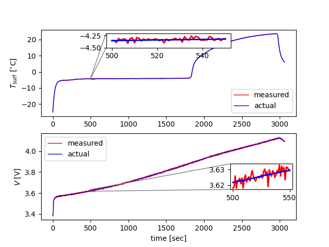
Figure 5: Actual and measured system outputs with $T_{\mathrm{amb}}=-25$ ${}^{\circ}\text{C}$.

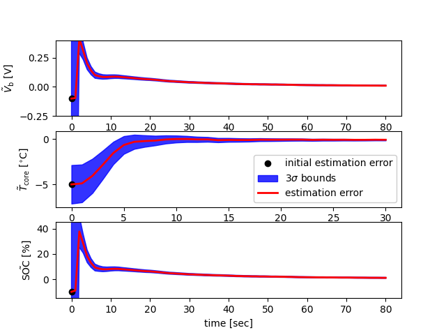
Figure 6: The trajectory segment of the estimation errors on unmeasurable states $V_{\mathrm{b}}$, $T_{\mathrm{core}}$ and $\mathrm{SOC}$ with $T_{\mathrm{amb}}=25$ ${}^{\circ}\text{C}$.

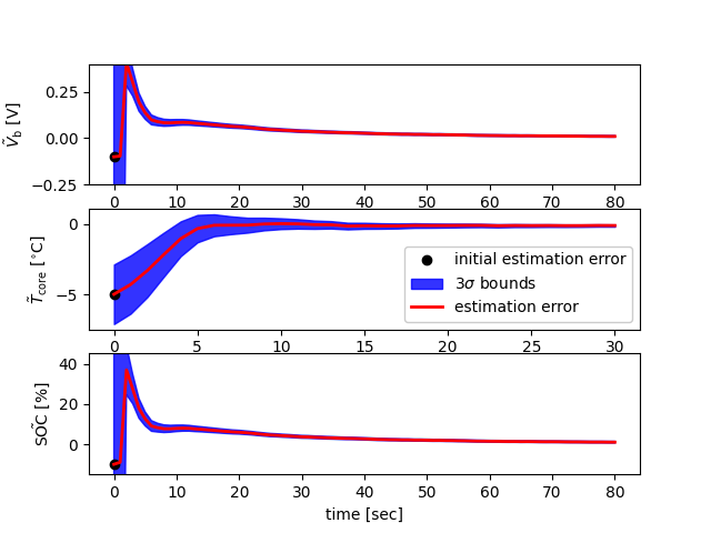
Figure 7: The trajectory segment of the estimation errors on unmeasurable states $V_{\mathrm{b}}$, $T_{\mathrm{core}}$ and $\mathrm{SOC}$ with $T_{\mathrm{amb}}=70$ ${}^{\circ}\text{C}$.

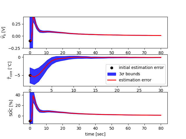
Figure 8: The trajectory segment of the estimation errors on unmeasurable states $V_{\mathrm{b}}$, $T_{\mathrm{core}}$ and $\mathrm{SOC}$ with $T_{\mathrm{amb}}=-25$ ${}^{\circ}\text{C}$.

The initial estimates on the unmeasurable states $V_{\mathrm{b}}$ and $T_{\mathrm{core}}$ are randomly initialized within $[V_{\mathrm{b}}(0)-0.1\mathrm{V},V_{\mathrm{b}}(0)+0.1\mathrm{V}]$ and $[T_{\mathrm{core}}(0)-5\ ^{\circ}\text{C},T_{\mathrm{core}}(0)+5\ ^{\circ}\text{C}]$, respectively. Note that the initial estimate error on $V_{\mathrm{b}}$ is relatively large since $V_{\mathrm{b}}$ varies between $[0\mathrm{V},1\mathrm{V}]$. The initial estimates of the measurable states are given by the initial measurements. For each $T_{\mathrm{amb}}$, the proposed EKF-based output-feedback MPC runs 20 trials with random initial estimates to verify its effectiveness.

The estimation errors for the unmeasurable states $V_{\mathrm{b}}$, $T_{\mathrm{core}}$ and $\mathrm{SOC}$ with different $T_{\mathrm{amb}}$ are illustrated in Fig. 6 - Fig. 8, where black dots indicate the initial state estimate; blue buffers indicate the estimation error plus and minus 3 times of standard deviation $\sigma$ given the estimate covariance $\boldsymbol{P}_{i|i}$. A small 3$\sigma$ error bound indicates that a 99.7% confidence interval of the state estimate is compact around the true state value. According to Fig. 6 - Fig. 8, both the state estimates and the $3\sigma$ error bound converge within about 80 s. Table VIII summarizes the EKF estimation error for unmeasurable states, which validates the EKF’s effectiveness.

Table VIII: EKF Estimation Error

State†	$T_{\mathrm{amb}}$	mean $\pm$ std	quartiles‡
$V_{\mathrm{b}}$	25 ∘C	$0.0012\pm 0.0064$	0.0003, 0.0007, 0.0011
$V_{\mathrm{s}}$	25 ∘C	$0.0008\pm 0.0018$	0.0003, 0.0006, 0.0009
$T_{\mathrm{core}}$	25 ∘C	$0.0172\pm 0.1051$	0.0013, 0.0030, 0.0092
$\mathrm{SoC}$	25 ∘C	$0.11\%\pm 0.59\%$	0.03%, 0.06%, 0.11%
$V_{\mathrm{b}}$	70 ∘C	$0.0012\pm 0.0065$	0.0003, 0.0007, 0.0011
$V_{\mathrm{s}}$	70 ∘C	$0.0008\pm 0.0018$	0.0003, 0.0006, 0.0009
$T_{\mathrm{core}}$	70 ∘C	$0.0092\pm 0.1070$	0.0011, 0.0023, 0.0047
$\mathrm{SoC}$	70 ∘C	$0.11\%\pm 0.60\%$	0.03%, 0.06%, 0.11%
$V_{\mathrm{b}}$	-25 ∘C	$0.0012\pm 0.0067$	0.0003, 0.0006, 0.0011
$V_{\mathrm{s}}$	-25 ∘C	$0.0008\pm 0.0018$	0.0003, 0.0005, 0.0009
$T_{\mathrm{core}}$	-25 ∘C	$0.0174\pm 0.1087$	0.0018, 0.0056, 0.0186
$\mathrm{SoC}$	-25 ∘C	$0.11\%\pm 0.62\%$	0.03%, 0.06%, 0.11%

• error unit for $V_{\mathrm{b}}$, $V_{\mathrm{s}}$, $T_{\mathrm{core}}$, and $\mathrm{SoC}$ are V, V, ^∘C, and %, respectively

• 25th, 50th, 75th percentile

The charging performance for all cases is summarized in Table IX. Comparing with the performance of P1 in Table III - Table V, both the computational time and the charging time from Table IX are longer than those of the state-feedback MPC. One contributing factor is the conservative revision of the Li-ion concentration gradient constraint (28), which includes a safety margin to account for estimation error and measurement noise. To illustrate this, consider the trajectory of $V_{\mathrm{s}}(t)-V_{\mathrm{b}}(t)$ vs $\beta_{1}\mathrm{SoC}(t)+\beta_{2}$ with $T_{\mathrm{amb}}=70$ ^∘C, as shown in Fig. 9. In Fig. 3, the same trajectory of $V_{\mathrm{s}}(t)-V_{\mathrm{b}}(t)$ without any noise or uncertainty approaches the boundary of $\beta_{1}\mathrm{SoC}(t)+\beta_{2}$ as SoC exceeds about 70%. However, when using output-feedback MPC with noise and uncertainty, the actual $V_{\mathrm{s}}(t)-V_{\mathrm{b}}(t)$ could exceed this boundary. Therefore, the 5% safety margin in (28) prevents constraint violation, but it also slows down the charging process due to the reduced concentration gradient.

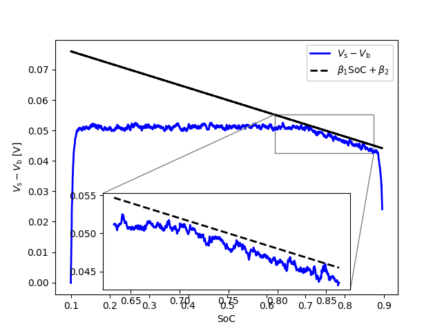
Figure 9: The trajectory of $V_{\mathrm{s}}(t)-V_{\mathrm{b}}(t)$ vs $\beta_{1}\mathrm{SoC}(t)+\beta_{2}$ with $T_{\mathrm{amb}}=70$ ${}^{\circ}\text{C}$.

On the other hand, the charging success rate is 100% for all the trials. As for constraint violations, for three $T_{\mathrm{amb}}$, the average time duration percentage that violates constraints is 0.0%$\pm$0.0%, 0.0%$\pm$0.0%, and 0.0033%$\pm$0.0144%, respectively. The maximum constraint violation is less than 0.1% of its upper bound, which might be caused by the measurement or numerical noises. The numerical experiments above validate the effectiveness of the proposed EKF-based output-feedback MPC under extreme ambient temperatures.

In this subsection, the proposed output-feedback MPC directly cold-starts with a relatively large estimation error. One practical approach is to initially run EKF independently for a period, allowing it to reduce the initial estimation error. Subsequently, the MPC algorithm can be initiated for charging. Details are referred to in the literature related to the separation principle [36, 37, 38].

Table IX: Battery Charging Result with EKF-Based Output-Feedback MPC

$T_{\mathrm{chg}}$ [s]	Energy [kJ]	Efficiency [%]	$T_{\mathrm{comp}}$ [ms]
3019.55$\pm$21.75	39.64$\pm$0.27	81.81$\pm$0.08	$30.41\pm 5.37$
3017.30$\pm$20.90	44.43$\pm$0.31	72.98$\pm$0.03	$27.94\pm 4.53$
3041.30$\pm$20.31	48.30$\pm$0.32	67.18$\pm$0.06	$33.09\pm 7.02$

• $T_{\mathrm{amb}}=25\ ^{\circ}\text{C},\ 70\ ^{\circ}\text{C},\ -25\ ^{\circ}\text{C}$ from top to bottom

VI Conclusion and Future Work

This paper explores integrated control strategies for fast charging and active thermal management of LiBs under extreme ambient temperatures. Firstly, a control-oriented thermal-NDC model is introduced to describe the electrical and thermal dynamics of LiBs, including the impact from both an active thermal source and ambient temperature. Secondly, a state-feedback MPC algorithm is developed to concurrently perform fast charging and active thermal management.

Thirdly, numerical experiments are conducted to validate the proposed state-feedback MPC algorithm under extreme ambient temperatures. These experiments demonstrate that heating the battery can enhance fast charging, which is consistent with the literature. By explicitly incorporating a higher desired battery core temperature into the MPC’s objective function, the algorithm achieves the fastest charging speed. However, with a suitable prediction horizon, an objective function without explicit heating can achieve a balanced performance across various indices. Finally, the proposed thermal-NDC model is rewritten properly to enable an EKF design for battery state estimation. An EKF-based output-feedback MPC algorithm is then proposed and validated through numerical experiments under extreme ambient temperatures.

The proposed thermal-NDC model is built upon the battery charging and discharging data, utilizing a maximum current of 1.5 C. As noted by [8, 19], applications such as eVTOL aircraft and EVs require high C-rate charging, which leads to significant heat generation and poses potentially a bigger concern on system safety. One avenue for future work is to develop battery model suitable for higher charging currents. Another future direction involves developing integrated charging and thermal management strategies for high C-rate scenarios. This may also require detailed modeling of actuators in the heating and cooling system.

References

- [1] A. Khaligh and Z. Li, “Battery, ultracapacitor, fuel cell, and hybrid energy storage systems for electric, hybrid electric, fuel cell, and plug-in hybrid electric vehicles: State of the art,” IEEE Transactions on Vehicular Technology, vol. 59, no. 6, pp. 2806–2814, 2010.
- [2] J. B. Goodenough and K.-S. Park, “The li-ion rechargeable battery: a perspective,” Journal of the American Chemical Society, vol. 135, no. 4, pp. 1167–1176, 2013.
- [3] J. B. Goodenough, “Energy storage materials: a perspective,” Energy Storage Materials, vol. 1, pp. 158–161, 2015.
- [4] Y. Wang, H. Fang, L. Zhou, and T. Wada, “Revisiting the state-of-charge estimation for lithium-ion batteries: A methodical investigation of the extended kalman filter approach,” IEEE Control Systems Magazine, vol. 37, no. 4, pp. 73–96, 2017.
- [5] P. Ramadass, B. Haran, P. M. Gomadam, R. White, and B. N. Popov, “Development of first principles capacity fade model for li-ion cells,” Journal of the Electrochemical Society, vol. 151, no. 2, p. A196, 2004.
- [6] C.-Y. Wang, G. Zhang, S. Ge, T. Xu, Y. Ji, X.-G. Yang, and Y. Leng, “Lithium-ion battery structure that self-heats at low temperatures,” Nature, vol. 529, no. 7587, pp. 515–518, 2016.
- [7] X.-G. Yang, G. Zhang, S. Ge, and C.-Y. Wang, “Fast charging of lithium-ion batteries at all temperatures,” Proceedings of the National Academy of Sciences, vol. 115, no. 28, pp. 7266–7271, 2018.
- [8] X.-G. Yang, T. Liu, S. Ge, E. Rountree, and C.-Y. Wang, “Challenges and key requirements of batteries for electric vertical takeoff and landing aircraft,” Joule, vol. 5, no. 7, pp. 1644–1659, 2021.
- [9] P. Sun, R. Bisschop, H. Niu, and X. Huang, “A review of battery fires in electric vehicles,” Fire technology, vol. 56, pp. 1361–1410, 2020.
- [10] R. Klein, N. A. Chaturvedi, J. Christensen, J. Ahmed, R. Findeisen, and A. Kojic, “Electrochemical model based observer design for a lithium-ion battery,” IEEE Transactions on Control Systems Technology, vol. 21, no. 2, pp. 289–301, 2012.
- [11] T. Weaver, A. Allam, and S. Onori, “A novel lithium-ion battery pack modeling framework-series-connected case study,” in 2020 American Control Conference (ACC). IEEE, 2020, pp. 365–372.
- [12] N. Tian, H. Fang, J. Chen, and Y. Wang, “Nonlinear double-capacitor model for rechargeable batteries: Modeling, identification, and validation,” IEEE Transactions on Control Systems Technology, vol. 29, no. 1, pp. 370–384, 2020.
- [13] G. L. Plett, Battery management systems, Volume I: Battery modeling. Artech House, 2015, vol. 1.
- [14] H. He, R. Xiong, and J. Fan, “Evaluation of lithium-ion battery equivalent circuit models for state of charge estimation by an experimental approach,” Energies, vol. 4, no. 4, pp. 582–598, 2011.
- [15] V. Johnson, “Battery performance models in advisor,” Journal of Power Sources, vol. 110, no. 2, pp. 321–329, 2002.
- [16] H. Fang, Y. Wang, and J. Chen, “Health-aware and user-involved battery charging management for electric vehicles: Linear quadratic strategies,” IEEE Transactions on Control Systems Technology, vol. 25, no. 3, pp. 911–923, 2016.
- [17] X. Lin, H. E. Perez, S. Mohan, J. B. Siegel, A. G. Stefanopoulou, Y. Ding, and M. P. Castanier, “A lumped-parameter electro-thermal model for cylindrical batteries,” Journal of Power Sources, vol. 257, pp. 1–11, 2014.
- [18] H. E. Perez, X. Hu, S. Dey, and S. J. Moura, “Optimal charging of li-ion batteries with coupled electro-thermal-aging dynamics,” IEEE Transactions on Vehicular Technology, vol. 66, no. 9, pp. 7761–7770, 2017.
- [19] N. Biju and H. Fang, “Battx: An equivalent circuit model for lithium-ion batteries over broad current ranges,” Applied Energy, vol. 339, p. 120905, 2023.
- [20] A. A.-H. Hussein and I. Batarseh, “A review of charging algorithms for nickel and lithium battery chargers,” IEEE Transactions on Vehicular Technology, vol. 60, no. 3, pp. 830–838, 2011.
- [21] Z. Lu and S. Mou, “Variable sampling mpc via differentiable time-warping function,” in 2023 American Control Conference (ACC), 2023, pp. 533–538.
- [22] R. Klein, N. A. Chaturvedi, J. Christensen, J. Ahmed, R. Findeisen, and A. Kojic, “Optimal charging strategies in lithium-ion battery,” in Proceedings of the 2011 American Control Conference. IEEE, 2011, pp. 382–387.
- [23] M. A. Xavier and M. S. Trimboli, “Lithium-ion battery cell-level control using constrained model predictive control and equivalent circuit models,” Journal of Power Sources, vol. 285, pp. 374–384, 2015.
- [24] C. Zou, X. Hu, Z. Wei, and X. Tang, “Electrothermal dynamics-conscious lithium-ion battery cell-level charging management via state-monitored predictive control,” Energy, vol. 141, pp. 250–259, 2017.
- [25] C. Zou, C. Manzie, and D. Nešić, “Model predictive control for lithium-ion battery optimal charging,” IEEE/ASME Transactions on Mechatronics, vol. 23, no. 2, pp. 947–957, 2018.
- [26] Q. Ouyang, J. Chen, J. Zheng, and H. Fang, “Optimal multiobjective charging for lithium-ion battery packs: A hierarchical control approach,” IEEE Transactions on Industrial Informatics, vol. 14, no. 9, pp. 4243–4253, 2018.
- [27] H. Fang, C. Depcik, and V. Lvovich, “Optimal pulse-modulated lithium-ion battery charging: Algorithms and simulation,” Journal of Energy Storage, vol. 15, pp. 359–367, 2018.
- [28] N. Tian, H. Fang, and Y. Wang, “Real-time optimal lithium-ion battery charging based on explicit model predictive control,” IEEE Transactions on Industrial Informatics, vol. 17, no. 2, pp. 1318–1330, 2020.
- [29] V. Azimi, A. Allam, and S. Onori, “Extending life of lithium-ion battery systems by embracing heterogeneities via an optimal control-based active balancing strategy,” IEEE Transactions on Control Systems Technology, 2022.
- [30] S. Feng, R. de Castro, and I. Ebrahimi, “Fast charging of batteries using cascade-control-barrier functions,” in 2023 American Control Conference (ACC). IEEE, 2023, pp. 2481–2486.
- [31] A. Hamednia, N. Murgovski, J. Fredriksson, J. Forsman, M. Pourabdollah, and V. Larsson, “Optimal thermal management, charging, and eco-driving of battery electric vehicles,” IEEE Transactions on Vehicular Technology, 2023.
- [32] J. A. Andersson, J. Gillis, G. Horn, J. B. Rawlings, and M. Diehl, “Casadi: a software framework for nonlinear optimization and optimal control,” Mathematical Programming Computation, vol. 11, pp. 1–36, 2019.
- [33] A. Wächter and L. T. Biegler, “On the implementation of an interior-point filter line-search algorithm for large-scale nonlinear programming,” Mathematical Programming, vol. 106, pp. 25–57, 2006.
- [34] R. Lowry, “Concepts and applications of inferential statistics,” 2014.
- [35] B. D. Anderson and J. B. Moore, Optimal filtering. Courier Corporation, 2012.
- [36] W. M. Wonham, “On the separation theorem of stochastic control,” SIAM Journal on Control, vol. 6, no. 2, pp. 312–326, 1968.
- [37] A. N. Atassi and H. K. Khalil, “A separation principle for the stabilization of a class of nonlinear systems,” IEEE Transactions on Automatic Control, vol. 44, no. 9, pp. 1672–1687, 1999.
- [38] T. T. Georgiou and A. Lindquist, “The separation principle in stochastic control, redux,” IEEE Transactions on Automatic Control, vol. 58, no. 10, pp. 2481–2494, 2013.