Why does the two-timescale Q-learning converge to different mean field solutions? A unified convergence analysis

Abstract

We revisit the unified two-timescale Q-learning algorithm as initially introduced by Angiuli et al. (2022). This algorithm demonstrates efficacy in solving mean field game (MFG) and mean field control (MFC) problems, simply by tuning the ratio of two learning rates for mean field distribution and the Q-functions respectively. In this paper, we provide a comprehensive theoretical explanation of the algorithm’s bifurcated numerical outcomes under fixed learning rates. We achieve this by establishing a diagram that correlates continuous-time mean field problems to their discrete-time Q-function counterparts, forming the basis of the algorithm. Our key contribution lies in the construction of a Lyapunov function integrating both mean field distribution and Q-function iterates. This Lyapunov function facilitates a unified convergence of the algorithm across the entire spectrum of learning rates, thus providing a cohesive framework for analysis.

Keywords: mean field games, mean field control, two-timescale algorithm, convergence analysis, reinforcement learning

1 Introduction

Reinforcement learning (RL) is a dynamic machine learning technique formalized through the framework of Markov Decision Processes (MDP), wherein an agent learns through interaction within an environment, relying on trial and error and feedback derived from its own actions and experiences (Sutton and Barto, 2018). RL has been prominent in artificial intelligence research in past decades and yields breakthroughs across diverse domains ranging from robotics (Kober et al., 2013), classical games (Mnih et al., 2013; Silver et al., 2016), to autonomous driving (Kiran et al., 2021). RL is closely related to the optimal control problems in the sense that it optimizes the decision-making processes by maximizing long-term cumulative rewards or minimizing cumulative costs under accessible policies (Bertsekas, 2019). Multi-agent reinforcement learning (MARL) extends the classical RL to scenarios involving multiple agents interacting within a shared environment, and we refer to survey works (Busoniu et al., 2008; Zhang et al., 2021) for its fundamental background. Despite its empirical success, the scalability of MARL with respect to the number of agents remains to be a key issue (Hernandez-Leal et al., 2019).

One approach to tackle the curse of scalability is to consider MARL in the regime with a large number of homogeneous agents. In this paradigm, mean field formulations provide a mathematical framework to model and analyze large-scale interacting particle systems independent of the number of agents $N$. Particularly, we focus on mean field game (MFG) and mean field control (MFC) problems as their theory has been developed rapidly in recent years. Mean field games, initially introduced by Lasry and Lions (2007) and Caines et al. (2006), are non-cooperative $N$-player games aim to find a Nash equilibrium where no individual agent can unilaterally improve the outcome by changing strategies. On the other hand, a mean field control problem has a central planner to find the collective optimum in a cooperative game within a large population. We refer to books Bensoussan et al. (2013) and Carmona and Delarue (2018) for further details of both MFG and MFC.

In the past years, solving stochastic control and games using model-free RL algorithms has gained a lot of interests, if one wants the agent to learn the optimal policy by directly interacting with the system without inferring the model parameters. We refer to (Hu and Laurière, 2023; Laurière et al., 2022) for a comprehensive review of recent developments. To learn MFG and MFC solutions, there are numerous algorithms available including but not limited to policy gradient based methods (Bhandari and Russo, 2024; Carmona et al., 2019; Williams, 1992), actor-critic methods for linear-quadratic models (Fu et al., 2019; Yang et al., 2018; Wang et al., 2021), fixed point iterations relying on entropy-regularization (Cui and Koeppl, 2021; Guo et al., 2022), and value-based RL methods such as Q-learning (Angiuli et al., 2022; Angiulia et al., 2023; Carmona et al., 2023; Guo et al., 2019; Mguni et al., 2018; Subramanian and Mahajan, 2019; Zaman et al., 2023; Gu et al., 2021).

In this paper, we focus on the work by Angiuli et al. (2022) that proposed a unified RL algorithm combining the classical Q-learning updates (Watkins, 1989; Watkins and Dayan, 1992) with the two-timescale approach (Borkar, 1997). This two-timescale Q-learning algorithm updates the mean field distribution and the value function iteratively, and can converge to either the MFG or MFC solutions by adjusting the ratio of associated Robbins-Monro learning rates to zero or infinity. A natural question to ask is why this simple two-timescale algorithm can produce bifurcated numerical results by just tuning two learning rates. We attempt to answer this question by:

1. Building a complete roadmap connecting the discrete-time Q-learning algorithm to continuous-time Hamilton-Jacobi-Bellman (HJB) equations for both MFG and MFC. The corresponding HJB equations for MFG and MFC are different depending on whether the population distribution is fixed, while such dependence is not explicitly captured in the two-timescale Q-learning algorithm.

2. Providing a unified convergence of the two-timescale Q-learning algorithm covering all choices of fixed learning rates. Rather than focusing on the extreme regimes of learning rates ratios and qualitative analysis, we aim to explain the algorithm’s bifurcated numerical behaviors quantitatively using the unified convergence result.

1.1 Our contributions

For the first part of our work, we start from the continuous-time MFG and MFC value functions under stochastic control with infinite time horizon, and we give formulations of corresponding discrete-time value and Q-functions which the two-timescale Q-learning algorithm is built on. We provide a sequence of approximation results to verify connections in Fig. 1 with respect to the time discretization $h$.

For the second part, we construct a Lyapunov function integrating both mean field distribution and Q-function iterates from the two-timescale Q-learning algorithm and prove its convergence quantitatively. Our approach takes generic assumptions on the cost function and the transition kernel, in addition to assuming the transition kernel satisfying a uniform Doeblin’s condition. The contraction of the constructed Lyapunov function exhibits explicit dependence on the two-timescale learning rates, thus explains how the two-timescale Q-learning algorithm can produce different solutions by tuning learning rates.

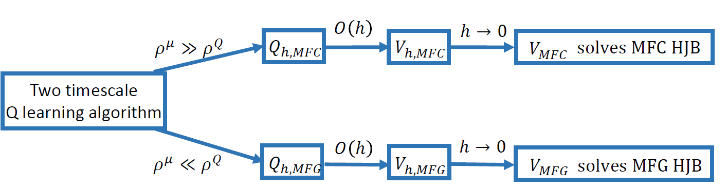
Figure 1: The diagram that links two-timescale Q-learning algorithm with optimal value functions solving HJB equations.

1.2 Related works

We mention several works related to our approach. We build the convergence diagram as in Fig. 1 since there is no continuous-time limit for the Q-learning iterations (Tallec et al., 2019). In the continuous-time setting where we can seek for differences of MFG and MFC in the HJB equations, the Q-function from the algorithm becomes ill-posed and collapses to the value function that is independent of actions. To analyze the continuous-time counterpart of Q-learning, Kim et al. (2021) restricts the action process to be Lipschitz continuous so that Q-learning becomes a policy evaluation problem with the state-action pair as the new state variable. Jia and Zhou (2023) and Wang et al. (2020) consider and analyze the entropy-regularized, exploratory diffusion process formulation which approximates the classical Q-function independent of time discretization. We list a few other papers (Kim and Yang, 2020; Gu et al., 2016; Jiang and Jiang, 2015; Palanisamy et al., 2014; Vamvoudakis, 2017) regarding general continuous-time RL.

On the other hand, our unified convergence of the two-timescale Q-learning algorithm takes motivations from the community that studies bi-level optimization. One problem somewhat related to setups in this paper is the linear quadratic regulator (LQR) in RL, and there have been many works studying two-timescale actor-critic algorithms for solving the LQR problem (Konda and Tsitsiklis, 1999; Zhou and Lu, 2023; Yang et al., 2019; Zeng et al., 2021). In particular, our Lyapunov function construction is inspired by Zhou and Lu (2023) who constructed a Lyapunov function involving both the critic error and the actor loss, although our goal is different from Zhou and Lu (2023): We try to find the fixed point of mean field problems, while Zhou and Lu (2023) aims to solve optimization problems.

We also mention that a recent paper by Angiuli et al. (2023) applies the theory of stochastic approximation (Borkar, 1997) to the two-timescale Q-learning algorithm, and they showed the algorithm convergence in extreme regimes where the ratio of learning rates is either zero or infinity. Compared to Angiuli et al. (2023), our approach of using the Lyapunov function is new and takes care of all ranges of learning rate ratios. Moreover, the convergence in Angiuli et al. (2023) is qualitative while our result is quantitative.

1.3 Organization

The paper is organized as follows. In Section 2, we review the formulations of the mean field game and mean field control problem that are the focus of our study. In Section 3, we outline the discrete value functions and Q-functions for MFG and MFC in bounded state and action spaces, and we review the continuous-time value functions solving the HJB equations derived in unbounded state and action spaces. A sequence of approximation errors between various formulations are provided. In Section 4, we revisit the two-timescale Q-learning algorithm and illustrate its bifurcated numerical behaviors by a toy example. In Section 5, we conduct the unified convergence analysis for the two-timescale Q-learning algorithm. Lastly, the numerical experiments that verifying the algorithm are provided in Section 6.

Notations

Throughout the paper, we use $\|\cdot\|$ to denote the Euclidean norm;
$\|Q(\cdot,\cdot)\|_{\infty}:=\sup_{x\in\mathcal{X},a\in\mathcal{A}}|Q(x,a)|$; $\|\mu\|_{p}=\big{(}\sum_{x\in\mathcal{X}}\mu(x)^{p}\big{)}^{1/p}$, and the total variation norm is $\|\mu\|_{\text{TV}}=\sup_{A\subseteq\mathcal{X}}\big{|}\sum_{x\in A}\mu(x)\big{|}$.

Acknowledgments

JA would like to express thanks to Mo Zhou, Lei Li, Yingzhou Li, and Jiequn Han for fruitful discussions. This work was done during YW’s visit of Duke University and Rhodes Information Initiative at Duke. YX was partially supported by the Project of Hetao Shenzhen-HKUST Innovation Cooperation Zone HZQB-KCZYB-2020083.

2 Background

We consider the Markov Decision Process (MDP) (Bellman, 1957; Watkins, 1989) with finite state and action spaces, which we denote by $\mathcal{X}$ and $\mathcal{A}$ respectively. $\mathcal{P}(\mathcal{X})$ is the space of probability measures on $\mathcal{X}$. The transition probability kernel can be viewed as a function

$$p:\mathcal{X}\times\mathcal{X}\times\mathcal{A}\times\mathcal{P}(\mathcal{X})\to[0,1],\quad(x,x^{\prime},a,\mu)\mapsto p(x^{\prime}\mid x,a,\mu),$$ (2.1)

which is, under the population distribution $\mu$, the probability of jumping from state $x$ to state $x^{\prime}$ using action $a$. Let $f:\mathcal{X}\times\mathcal{A}\times\mathcal{P}(\mathcal{X})\to\mathbb{R}_{+}$ be a running cost function. $f(x,a,\mu)$ can be interpreted as the one-step cost incurred by an agent at state $x$ to take an action $a$, when the population distribution is $\mu$.

There are various formulations of MFG and MFC problems available in the literature. In Angiuli et al. (2022), three formulations in the infinite horizon were presented: asymptotic, non-asymptotic, and stationary. We will focus on the asymptotic formulations given in Angiuli et al. (2022), since then the problem faced by an infinitesimal agent among the crowd can be viewed as a MDP parameterized by the population distribution. We refer other infinite time horizon formulations to Angiuli et al. (2022) and the finite time horizon version to Angiulia et al. (2023) if readers are interested.

We start by reviewing the formulation of stochastic control problems in the infinite time horizon with continuous state space. Let $(\Omega,\mathcal{F},\mathbb{P})$ be a probability space accompanied with filtration $\{\mathcal{F}_{t}\}_{t\geq 0}$ generated by a standard $n$-dimensional Brownian motion $B=\{B_{t}\}_{t\geq 0}$. For any time $t$, one has the state $X_{t}\in\mathcal{X}\subseteq{\mathbb{R}}^{d}$ following the McKean–Vlasov dynamics (i.e., distribution-dependent dynamics) and the Markovian control $\alpha_{t}=\alpha(X_{t}):\mathcal{X}\to\mathcal{A}\subseteq{\mathbb{R}}^{k}$. Given Borel-measurable functions

$$b:\mathcal{X}\times\mathcal{A}\times\mathcal{P}(\mathcal{X})\to{\mathbb{R}}^{d},\quad\sigma:\mathcal{X}\times\mathcal{A}\times\mathcal{P}(\mathcal{X})\to{\mathbb{R}}^{d\times n}$$ (2.2)

that satisfy necessary conditions for the well-posedness (see Section 3.2 for details). The stochastic control problem is that an agent controls her state $X$ via a sequence of actions (policy) $\alpha$ with the goal of minimizing the expected discounted cost

$$\inf_{\alpha}J^{\mu}(\alpha) =\inf_{\alpha}\mathbb{E}\left[\int_{0}^{\infty}e^{-\gamma t}f(X_{t},\alpha_{t},\mu_{t})dt\right],$$ (2.3)

s.t. $$dX_{t}=b(X_{t},\alpha_{t},\mu_{t})dt+\sigma(X_{t},\alpha_{t},\mu_{t})dB_{t},\quad\quad X_{0}\sim\mu_{0},$$

with a discount factor $\gamma>0$ and the probability measure flow $\mu_{t}$ starting from $\mu_{0}=\mathcal{P}[X_{0}]$, i.e., $\mu_{t}$ is the law of $X_{t}$. For more general versions of stochastic control problems and associated theory, we refer readers to the book by Carmona and Delarue (2018).

The above general formulation with stochastic differential equation (SDE) control is based on unbounded state space $\mathcal{X}$. To be closely connected with reinforcement learning with a bounded state space $\mathcal{X}$ and an action space $\mathcal{A}$, we would consider MFG and MFC problems on discrete state space in the asymptotic sense following (Angiuli et al., 2022, Section 2.2). In this setup, the control does not depend on time but only on the state, since the transition probability $p$ and the cost function $f$ only depend on the limiting distributions other than time. The SDE control is replaced by the transition probability $p$, and the discount prefactor $e^{-\gamma t}$ is replaced by $r^{k}$ for some $r\in(0,1)$.

Mean Field Game (MFG)

Solving a MFG problem is to find a Nash equilibrium $(\hat{\alpha},\hat{\mu})$ in a non-cooperative game by following:

1. Fix a probability distribution $\hat{\mu}\in\mathcal{P}(\mathcal{X})$ and solve the standard stochastic control problem

   $$\inf_{\alpha}J^{\hat{\mu}}(\alpha) =\inf_{\alpha}\mathbb{E}\left[\sum_{k=0}^{\infty}r^{k}f(X_{k}^{\alpha,\hat{\mu}},\alpha(X_{k}^{\alpha,\hat{\mu}}),\hat{\mu})\right],$$ (2.4)

   s.t. $$X_{k+1}^{\alpha,\hat{\mu}}\sim p(\cdot\mid X_{k}^{\alpha,\hat{\mu}},\alpha(X_{k}^{\alpha,\hat{\mu}}),\hat{\mu}),\quad X_{0}^{\alpha,\hat{\mu}}\sim\mu_{0},$$

2. Given the optimal control $\hat{\alpha}$, find the fixed point $\hat{\mu}$ such that

   $$\hat{\mu}=\lim_{k\to\infty}\mathcal{P}[X^{\hat{\alpha},\hat{\mu}}_{k}].$$

Mean Field Control (MFC)

Different from MFG that has fixed $\mu$ in the first step, the population distribution $\mu_{k}=\mathcal{P}[X_{k}^{\alpha}]$ in MFC changes instantaneuously when $\alpha$ changes. The asymptotic version of the problem is thus written as

$$\inf_{\alpha}J(\alpha) =\inf_{\alpha}\mathbb{E}\left[\sum_{k=0}^{\infty}r^{k}f(X_{k}^{\alpha},\alpha_{k},\lim_{k\to\infty}\mathcal{P}[X_{k}^{\alpha}])\right],$$ (2.5)

s.t. $$X_{k+1}^{\alpha}\sim p(\cdot\mid X_{k}^{\alpha},\alpha(X_{k}^{\alpha}),\lim_{k\to\infty}\mathcal{P}[X_{k}^{\alpha}]),\quad X_{0}^{\alpha}\sim\mu_{0},$$

so that the control $\alpha$ is independent of time, as $p$ and $f$ depend only on the limiting distribution (as $k\to\infty$).

We emphasize that the main difference between the two is that in MFG, the distribution $\mu$ is prescribed when the optimal control is solved (and hence the superscript $\mu$ in the notation), while in MFC, the distribution depends on the choice of $\alpha$, when the policy is optimized.

3 Value functions and Q-functions

We first recall formulations of value functions and Q-functions in both continuous and discrete time. With these, we establish the sequence of approximations in Fig. 1 from $Q_{h}$ which satisfies the Bellman equation to $V$ which solves the HJB equation.

3.1 Value functions

We recall the classical continuous-time value functions for mean field game (MFG) and mean field control (MFC) problems, respectively. The value function of the MFG, with any fixed population distribution $\mu\in\mathcal{P}(\mathcal{X})$, is written as

$$V_{\text{MFG}}^{\alpha,\mu}(x)=\mathbb{E}\left[\int_{0}^{\infty}e^{-\gamma s}f(X_{s}^{\alpha,\mu},\alpha_{s},\mu)ds\bigg{|}X_{0}=x\right].$$ (3.1)

On the other hand, the value function of the MFC, different from MFG, has population distribution $\mu_{t}\in\mathcal{P}(\mathcal{X})$ changing over time depending on the control. For asymptotic MFC, it is defined as

$$V_{\text{MFC}}^{\alpha}(x)=\mathbb{E}\left[\int_{0}^{\infty}e^{-\gamma s}f(X_{s}^{\alpha},\alpha_{s},\lim_{t\to\infty}\mathcal{P}[X_{t}^{\alpha}])ds\bigg{|}X_{0}=x\right].$$ (3.2)

For formulations (3.1) or (3.2), the dynamics of $X_{t}$ follows a Markov process with

$$X_{t}\sim p(\cdot\mid X_{t^{\prime}},\alpha(X_{t^{\prime}}),\mu)\quad\text{for}~{}t^{\prime}<t,$$ (3.3)

where $\mu$ is fixed for MFG and $\mu=\lim_{t\to\infty}\mathcal{P}[X_{t}]$ for MFC (recall we consider the asymptotic MFC in this work).

Analogously, if we consider the discrete MDP $(\mathcal{X},\mathcal{A},e^{-\gamma h},f_{k})$ as a counterpart of the continuous-time MDP with time discretization $h$, and we use the notations $X_{k}\equiv X_{kh},\alpha_{k}\equiv\alpha_{kh}=\alpha(X_{k}),\mu_{k}\equiv\mu_{kh},f_{k}\equiv f(X_{k},\alpha_{k},\mu_{k})$, then given an admissible policy $\alpha$, the discrete value functions $V_{h}^{\alpha}$ for MFG has the form of

$$V_{h,\text{MFG}}^{\alpha,\mu}(x):=\mathbb{E}\left[h\sum_{k=0}^{\infty}e^{-k\gamma h}f(X_{k}^{\alpha,\mu},\alpha_{k},\mu)\bigg{|}X_{0}=x\right],$$ (3.4)

with the state $X_{k}^{\alpha,\mu}$ changes by

$$X_{k+1}^{\alpha,\mu}\sim p(\cdot\mid X_{k}^{\alpha,\mu},\alpha_{k},\mu).$$ (3.5)

Similarly, for MFC, we have the form

$$V_{h,\text{MFC}}^{\alpha}(x)=\mathbb{E}\left[h\sum_{k=0}^{\infty}e^{-k\gamma h}f(X_{k}^{\alpha},\alpha_{k},\lim_{k\to\infty}\mathcal{P}[X_{k}^{\alpha}])\bigg{|}X_{0}=x\right],$$ (3.6)

with the state $X_{k}^{\alpha}$ changes by

$$X_{k+1}^{\alpha}\sim p(\cdot\mid X_{k}^{\alpha},\alpha_{k},\lim_{k\to\infty}\mathcal{P}[X_{k}^{\alpha}]).$$ (3.7)

For (3.1) and (3.2), we can derive the optimal value functions by optimizing over policies $\alpha$:

$$V_{\text{MFG}}^{\mu}(x)=\inf_{\alpha}V_{\text{MFG}}^{\mu,\alpha}(x),\quad V_{\text{MFC}}(x)=\inf_{\alpha}V_{\text{MFC}}^{\alpha}(x),$$ (3.8)

Similarly, for (3.4) and (3.6), the discrete optimal value functions are defined as

$$V_{h,\text{MFG}}^{\mu}(x)=\inf_{\alpha_{h}}V_{h,\text{MFG}}^{\mu,\alpha}(x),\quad V_{h,\text{MFC}}(x)=\inf_{\alpha_{h}}V_{h,\text{MFC}}^{\alpha}(x).$$ (3.9)

In addition, we introduce the assumption on the cost function $f$ that will be used throughout the paper.

Assumption 1

We assume that the cost function $f:\mathcal{X}\times\mathcal{A}\times\mathcal{P}(\mathcal{X})\rightarrow\mathbb{R}$ is bounded and Lipschitz continuous in $\mu$, in the sense that there exists a constant $L_{\mu}>0$ such that for every $(x,a)\in\mathcal{X}\times\mathcal{A}$,

$$\big{|}f(x,a,\mu_{1})-f(x,a,\mu_{2})\big{|}\leq L_{\mu}\|\mu_{1}-\mu_{2}\|_{\text{TV}}\quad\text{for any }\mu_{1},\mu_{2}\in\mathcal{P}(\mathcal{X}).$$ (3.10)

3.2 HJB equations with SDE controls

While for most of this work, we consider discrete state space, we study in this section the continuous state space analog, where the state dynamics is given by stochastic differential equations (controlled diffusion)

$$dX_{t}=b(X_{t},\alpha_{t},\mu_{t})dt+\sigma(X_{t},\alpha_{t},\mu_{t})dB_{t}.$$ (3.11)

We use this setup to review the familiar Hamilton-Jacobi-Bellman equations, which would shed light on the difference between MFG and MFC in the continuous-time solution viewpoint. Furthermore, our numerical experiments in Section 6 are based on discretizations of the SDE.

For continuous state space models, we require some additional assumptions to ensure the wellposedness of the problem.

Assumption 2

Given an unbounded state space $\mathcal{X}$, we assume that the cost function $f:\mathcal{X}\times\mathcal{A}\times\mathcal{P}(\mathcal{X})\rightarrow\mathbb{R}$ is bounded and measurable. For any fixed $\mu\in\mathcal{P}(\mathcal{X})$, $f$ is Lipschitz continuous in $x,a$, in the sense that there exist constants $L_{x},L_{\alpha}>0$ such that

$$\big{|}f(x_{1},\alpha_{1},\mu)-f(x_{2},\alpha_{2},\mu)\big{|}\leq L_{x}\|x_{1}-x_{2}\|+L_{\alpha}\|\alpha_{1}-\alpha_{2}\|\quad\text{for any }x_{1},x_{2}\in\mathcal{X},~{}a_{1},a_{2}\in\mathcal{A}.$$ (3.12)

Assumption 3

We assume that for any $(x,a,\mu)\in\mathcal{X}\times\mathcal{A}\times\mathcal{P}(\mathcal{X})$, both $b(x,a,\mu)$ and $\sigma(x,a,\mu)$ are measurable, bounded, and Lipschitz in $x,a$, which means that there exist constants $K_{x},K_{\alpha}>0$, and for every $\mu\in\mathcal{P}(\mathcal{X})$, it holds uniformly that

$$\|b(x^{\prime},a^{\prime},\mu)-b(x,a,\mu)\|\leq K_{x}\|x^{\prime}-x\|+K_{\alpha}\|a^{\prime}-a\|,$$ (3.13)

$$\|\sigma(x^{\prime},a^{\prime},\mu)-\sigma(x,a,\mu)\|\leq K_{x}\|x^{\prime}-x\|+K_{\alpha}\|a^{\prime}-a\|.$$

Moreover, both $b(x,a,\mu)$ and $\sigma(x,a,\mu)$ are differentiable in $x$ and $a$.

Given the optimal value functions $V$, one can obtain the HJB equations for MFG and MFC by following the derivations in Chapter 3 and Chapter 4 of Bensoussan et al. (2013) respectively. For simplicity, we give the statement with constant $\sigma(x,a)\equiv\sigma>0$.

Definition 1

We say $f(x,a,\mu)$ is differentiable in $\mu$ if the first variation

$$\frac{d}{d\epsilon}f(x,a,\mu+\epsilon m)\Big{|}_{\varepsilon=0}:=\int_{\mathcal{X}}\frac{\delta f(x,a,\mu)}{\delta\mu}(\xi)\,m(d\xi)$$ (3.14)

exists, for any $m\in\mathcal{P}(\mathcal{X})$.

Theorem 2 (Bensoussan et al. (2013))

Under Assumptions 1, 2, and 3, with the Hamiltonian

$$H(x,\mu,q):=\inf_{\alpha}\left\{q\cdot b(x,\alpha,\mu)+f(x,\alpha,\mu)\right\},$$ (3.15)

the optimal value function $V_{\text{MFG}}^{\mu}$ for asymptotic MFG satisfies the HJB equation

$$-\gamma V^{\mu}(x)+\frac{\sigma^{2}\operatorname{Tr}{\nabla^{2}V^{\mu}(x)}}{2}+H(x,\mu,\nabla V^{\mu}(x))=0.$$ (3.16)

On the other hand, the optimal value function $V_{\text{MFC}}$ for asymptotic MFC satisfies the HJB equation

$$-\gamma V(x)++\frac{\sigma^{2}\operatorname{Tr}{\nabla^{2}V(x)}}{2}+H(x,\mu,\nabla V(x))+\int_{\mathcal{X}}\frac{\delta H(y,\mu,\nabla V(y))}{\delta\mu}(x)\,\mu(dy)=0,$$ (3.17)

coupled with $\mu$ solving the stationary Fokker-Planck equation

$$-\sum_{i=1}^{d}\frac{\partial}{\partial x_{i}}(b_{i}(x,\hat{\alpha},\mu)\mu)+\frac{\sigma^{2}}{2}\Delta\mu=0,$$ (3.18)

where $\hat{\alpha}$ is the optimal control for the Lagrangian in (3.15).

From the above HJB equations, it is straightforward to see that, in general $V_{\text{MFG}}^{\mu}$ and $V_{\text{MFC}}$ are different solutions, as in the case of MFC the HJB equation has an additional term due to the coupling with $\mu$. In next few sections, we will study how the two-timescale Q-learning algorithm converges to these different value functions.

The following results state that given any policy $\alpha$, the discrete value function is close to the continuous-time value function for sufficiently small $h$, which implies similar approximation results for optimal value functions.

Theorem 3

(Informal version of Theorem A.1) Under appropriate assumptions, under an given policy $\alpha$, for all $x\in{\mathcal{X}}$, one has approximations

$$\lim_{h\to 0}V_{h,\text{MFG}}^{\mu,\alpha}(x)=V_{\text{MFG}}^{\mu,\alpha}(x),\quad\lim_{h\to 0}V_{h,\text{MFC}}^{\alpha}(x)=V_{\text{MFC}}^{\alpha}(x).$$ (3.19)

The idea of the proof is standard by extending Lemma 1 in Tallec et al. (2019) to a stochastic version with additional assumptions. We defer the formal statement with convergence rates, as well as proof details to Appendix A.

Corollary 4

By Theorem 3 and taking the optimal control $\hat{\alpha}$, we have that the approximations for the optimal value functions

$$\lim_{h\to 0}V_{h,\text{MFG}}^{\mu}(x)=V_{\text{MFG}}^{\mu}(x),\quad\lim_{h\to 0}V_{h,\text{MFC}}(x)=V_{\text{MFC}}(x).$$ (3.20)

3.3 Q-functions

Following the context of asymptotic MFG (2.4) introduced in Angiuli et al. (2022), the discrete time Q-function (i.e., state-action value function) and optimal Q-function are defined as

$$Q_{h,\text{MFG}}^{\alpha,\mu}(x,a):=\mathbb{E}\left[h\sum_{k=0}^{\infty}e^{-k\gamma h}f(X_{k}^{\alpha,\mu},\alpha_{k},\mu)\bigg{|}X_{0}=x,\alpha_{0}=a\right],$$ (3.21)

$$Q^{\mu}_{h,\text{MFG}}(x,a):=\inf_{\alpha}Q_{h,\text{MFG}}^{\alpha,\mu}(x,a).$$

Optimizing over initial actions, we have that $V_{h,\text{MFG}}^{\mu}(x)=\inf_{a}Q_{h,\text{MFG}}^{\mu}(x,a)$ for any $x\in\mathcal{X}$. Moreover, as $\mu$ is fixed, by (Sutton and Barto, 2018, Equation (3.20)), $Q_{h,\text{MFG}}^{\mu}$ satisfies the Bellman equation

$$Q_{h,\text{MFG}}^{\mu}(x,a)=hf(x,a,\mu)+e^{-\gamma h}\sum_{x^{\prime}\in\mathcal{X}}p(x^{\prime}\mid x,a,\mu)\inf_{a^{\prime}}Q_{h,\text{MFG}}^{\mu}(x^{\prime},a^{\prime}).$$ (3.22)

On the other hand, the case of MFC is more complicated. In the context of asymptotic MFC (2.5), considering $\mu^{\alpha}$ to be the limiting distribution of the process $X_{t}^{\alpha}$ for an admissible policy $\alpha$, the discrete time modified Q-function introduced in Angiuli et al. (2022) is defined as

$$Q_{h,\text{MFC}}^{\alpha}(x,a):=hf(x,a,\mu^{\tilde{\alpha}})+\mathbb{E}\left[h\sum_{k=1}^{\infty}e^{-k\gamma h}f(X_{k}^{\alpha},\alpha_{k},\mu^{\alpha})\bigg{|}X_{0}=x,\alpha_{0}=a\right],$$ (3.23)

where

$$\mu^{\alpha}=\lim_{k\to\infty}\mathcal{P}[X_{k}^{\alpha}],\quad\quad\tilde{\alpha}(s)=\begin{cases}\alpha(s),\quad\text{if}~{}~{}s\neq x\\ a,\quad\quad~{}\text{if}~{}~{}s=x.\end{cases}$$ (3.24)

We mention that $\tilde{\alpha}$ is devised in such a form (3.24) in order to achieve policy improvement (Angiuli et al., 2022, Theorem 4 in Appendix C). Then the optimal Q-function $Q_{h,\text{MFC}}$ is

$$Q_{h,\text{MFC}}(x,a)=\inf_{\alpha}Q_{h,\text{MFC}}^{\alpha}(x,a),$$ (3.25)

which satisfies the Bellman equation

$$Q_{h,\text{MFC}}(x,a)=hf(x,a,\tilde{\mu}^{*})+e^{-\gamma h}\sum_{x^{\prime}\in\mathcal{X}}p(x^{\prime}\mid x,a,\tilde{\mu}^{*})\inf_{a^{\prime}}Q_{h,\text{MFC}}(x^{\prime},a^{\prime}),$$ (3.26)

for each $(x,a)\in\mathcal{X}\times\mathcal{A}$. The optimal control $\alpha^{*}(x)=\operatorname*{arg\,min}_{a\in\mathcal{A}}Q_{h,\text{MFC}}(x,a)$, and the control $\tilde{\alpha}^{*}$ is also defined as in (3.24). The modified population distribution $\tilde{\mu}^{*}$ is based on $\tilde{\alpha}^{*}$ in the sense that $\tilde{\mu}^{*}=\mu^{\tilde{\alpha}^{*}}$. Let us summarize the discrete time Q-function results for asymptotic MFC as follows.

Theorem 3.1 (Angiuli et al. (2022), Appendix C)

The Bellman equation for the discrete time Q-function $Q_{h,\text{MFC}}^{\alpha}$ is

$$Q_{h,\text{MFC}}^{\alpha}(x,a)=hf(x,a,\mu^{\tilde{\alpha}})+e^{-\gamma h}\mathbb{E}\left[Q_{h,\text{MFC}}^{\alpha}(X_{1},\alpha(X_{1}))|X_{0}=x,\alpha_{0}=a\right]$$ (3.27)

with $\tilde{\alpha}$ defined as in (3.24). Moreover, for any $x\in\mathcal{X}$, the value function is equivalent to the Q-function with the policy $\alpha$ in the form of

$$V_{h,\text{MFC}}^{\alpha}(x)=Q_{h,\text{MFC}}^{\alpha}(x,\alpha(x)).$$ (3.28)

The optimal Q-function $Q_{h,\text{MFC}}(x,a)=\inf_{\alpha}Q_{h,\text{MFC}}^{\alpha}(x,a)$ satisfies the Bellman equation

$$Q_{h,\text{MFC}}(x,a)=hf(x,a,\tilde{\mu}^{*})+e^{-\gamma h}\sum_{x^{\prime}\in\mathcal{X}}p(x^{\prime}\mid x,a,\tilde{\mu}^{*})\inf_{a^{\prime}}Q_{h,\text{MFC}}(x^{\prime},a^{\prime}),$$ (3.29)

with $\tilde{\mu}^{*}=\mu^{\tilde{\alpha}^{*}}$ and $\tilde{\alpha}^{*}$ being the modified control (3.24) of the optimal control $\alpha^{*}$.

Proof  All proofs can be found in (Angiuli et al., 2022, Appendix C). We review the proofs of the first two statements here and delegate the last one to the reference.

(Angiuli et al., 2022, Appendix C, Theorem 3) : By the tower property, the definition of (3.23) gives

$$Q_{h,\text{MFC}}^{\alpha}(x,a)=hf(x,a,\mu^{\tilde{\alpha}})+e^{-\gamma h}\mathbb{E}\left[\mathbb{E}\left[h\sum_{k=1}^{\infty}e^{-(k-1)\gamma h}f(X_{k},\alpha_{k},\mu^{\alpha})\bigg{|}X_{1}\right]\bigg{|}X_{0}=x,\alpha_{0}=a\right]$$

$$=hf(x,a,\mu^{\tilde{\alpha}})$$

$$\quad+e^{-\gamma h}\mathbb{E}\left[hf(X_{1},\alpha(X_{1}),\mu^{\alpha})+e^{-\gamma h}\mathbb{E}\left[h\sum_{k=2}^{\infty}e^{-(k-2)\gamma h}f(X_{k},\alpha_{k},\mu^{\alpha})\bigg{|}X_{1}\right]\bigg{|}X_{0}=x,\alpha_{0}=a\right]$$

$$=hf(x,a,\mu^{\tilde{\alpha}})+e^{-\gamma h}\mathbb{E}\left[Q_{h,\text{MFC}}^{\alpha}(X_{1},\alpha(X_{1}))|X_{0}=x,\alpha_{0}=a\right].$$

(Angiuli et al., 2022, Appendix C, Lemma 3): By the form of modified control (3.24), the discrete value function can be written as

$$V_{h,\text{MFC}}^{\alpha}(x) =hf(x,\alpha(x),\mu^{\tilde{\alpha}})+\mathbb{E}\left[h\sum_{k=1}^{\infty}e^{-k\gamma h}f(X_{k},\alpha_{k},\mu^{\alpha})\bigg{|}X_{0}=x,\alpha_{0}=\alpha(x)\right]$$

$$=Q_{h,\text{MFC}}^{\alpha}(x,\alpha(x)).$$

 

3.4 Approximation results for value functions

The Q-function is ill-posed for the continuous-time MDP (Tallec et al., 2019), as it becomes independent of actions when $h\to 0$. However, one can measure the difference between discrete value functions and Q-functions in terms of $h$, when the control $\alpha$ is fixed. Such a distance measure result can be found in (Tallec et al., 2019, Theorem 2) for MFG problems when the state is driven by the deterministic differential equation. Here, we provide similar results for both MFG and MFC under the McKean-Vlasov dynamics control, based on formulations (3.22), (3.27), and (3.28).

Theorem 3.2 (Difference between $Q_{h}^{\alpha}$ and $V_{h}^{\alpha}$)

Let ${\mathbbm{1}}_{x}$ be the unit point mass probability distribution over $\mathcal{X}$. Consider the infinitesimal generator $G$ given by

$$G(\cdot\mid x,a,\mu)=\lim_{h\to 0}\frac{p_{h}(\cdot\mid x,a,\mu)-{\mathbbm{1}}_{x}}{h}$$ (3.30)

being uniformly bounded for all $(x^{\prime},x,a,\mu)\in\mathcal{X}\times\mathcal{X}\times\mathcal{A}\times\mathcal{P}(\mathcal{X})$, and $p_{h}(\cdot\mid x,a,\mu)$ is the one-step transition probability with respect to the time step $h$. If $f$ is uniformly bounded over $\mathcal{X}\times\mathcal{A}\times\mathcal{P}(\mathcal{X})$, following the one-step McKean-Vlasov dynamics $x^{\prime}\sim p_{h}(\cdot\mid x,a,\mu)$, we have that

$$Q_{h,\text{MFG}}^{\mu,\alpha}(x,a)=V_{h,\text{MFG}}^{\mu,\alpha}(x)+O(h),$$ (3.31)

$$Q_{h,\text{MFC}}^{\alpha}(x,a)=V_{h,\text{MFC}}^{\alpha}(x)+O(h),$$

with sufficiently small $h>0$, for every $(x,a)\in\mathcal{X}\times\mathcal{A}$.

Proof  As $f$ is uniformly bounded, $V$ is also uniformly bounded over $\mathcal{X}$ by its formulations.

For MFG, the Bellman equation gives that

$$Q_{h,\text{MFG}}^{\mu,\alpha}(x,a) =hf(x,a,\mu)+e^{-\gamma h}\mathbb{E}\left[Q_{h,\text{MFG}}^{\mu,\alpha}(X_{1},\alpha(X_{1}))|X_{0}=x,\alpha_{0}=a\right]$$

$$=hf(x,a,\mu)+(1-\gamma h)\mathbb{E}\left[V_{h,\text{MFG}}^{\mu,\alpha}(x^{\prime})\right]+O(h^{2}),$$

with $X_{1}=x^{\prime}$ and sufficiently small $h$. Note that

$$\mathbb{E}\left[V_{h,\text{MFG}}^{\mu,\alpha}(x^{\prime})\right] =\sum_{x^{\prime}}V_{h,\text{MFG}}^{\mu,\alpha}(x^{\prime})p_{h}(x^{\prime}\mid x,a,\mu)$$ (3.32)

$$=V_{h,\text{MFG}}^{\mu,\alpha}(x)+\sum_{x^{\prime}}V_{h,\text{MFG}}^{\mu,\alpha}(x^{\prime})(p_{h}(x^{\prime}\mid x,a,\mu)-{\mathbbm{1}}_{x})$$

$$=V_{h,\text{MFG}}^{\mu,\alpha}(x)+\sum_{x^{\prime}}V_{h,\text{MFG}}^{\mu,\alpha}(x^{\prime})G(x^{\prime}\mid x,a,\mu)h+\lito(h)=V_{h,\text{MFG}}^{\mu,\alpha}(x)+O(h)$$

as the generator $G$ is uniformly bounded and $\mathcal{X}$ is finite. Therefore, by replacing $\mathbb{E}\left[V_{h,MFG}^{\mu,\alpha}(x^{\prime})\right]$ in the Bellman equation, we get

$$Q^{\mu,\alpha}_{h,\text{MFG}}(x,a)=hf(x,a,\mu)+(1-\gamma h)\big{(}V^{\mu,\alpha}_{h,\text{MFG}}(x)+O(h)\big{)}+O(h^{2})=V^{\mu,\alpha}_{h,\text{MFG}}(x)+O(h),$$

for sufficiently small $h$. The estimate for MFC is similar by just replacing $\mu$ by the limiting distribution $\mu^{\alpha}=\lim_{k\to\infty}\mathcal{P}[X_{k}^{\alpha}]$ under an admissible policy $\alpha$. The Bellman equation (3.27) combined with (3.28) gives

$$Q_{h,\text{MFC}}^{\alpha}(x,a) =hf(x,a,\mu^{\tilde{\alpha}})+e^{-\gamma h}\mathbb{E}\left[V_{h,\text{MFC}}^{\alpha}(x^{\prime})|X_{0}=x,\alpha_{0}=a\right]$$ (3.33)

$$=hf(x,a,\mu^{\tilde{\alpha}})+(1-\gamma h)\mathbb{E}\left[V_{h,\text{MFC}}^{\alpha}(x^{\prime})\right]+O(h^{2}),$$

for sufficiently small $h$. Since

$$\mathbb{E}\left[V_{h,\text{MFC}}^{\mu,\alpha}(x^{\prime})\right] =\sum_{x^{\prime}}V_{h,\text{MFC}}^{\mu,\alpha}(x^{\prime})p_{h}(x^{\prime}\mid x,a,\mu^{\alpha})$$ (3.34)

$$=V_{h,\text{MFC}}^{\mu,\alpha}(x)+\sum_{x^{\prime}}V_{h,\text{MFC}}^{\mu,\alpha}(x^{\prime})G(x^{\prime}\mid x,a,\mu^{\alpha})h+\lito(h)=V_{h,\text{MFC}}^{\mu,\alpha}(x)+O(h),$$

then the Bellman equation gives that

$$Q^{\alpha}_{h,\text{MFC}}(x,a)=hf(x,a,\mu^{\tilde{\alpha}})+(1-\gamma h)\big{(}V^{\alpha}_{h,\text{MFC}}(x)+O(h)\big{)}+O(h^{2})=V^{\alpha}_{h,\text{MFC}}(x)+O(h)$$

for sufficiently small $h$.  

Corollary 5

For discrete optimal value functions and Q-functions, by taking the infimum over all admissible policies $\alpha$, we have that

$$Q_{h,\text{MFG}}^{\mu}(x,a)=V_{h,\text{MFG}}^{\mu}(x)+O(h),$$ (3.35)

and

$$Q_{h,\text{MFC}}(x,a)=V_{h,\text{MFC}}(x)+O(h),$$ (3.36)

for sufficiently small $h>0$, for every $(x,a)\in\mathcal{X}\times\mathcal{A}$.

4 Two-timescale Q-learning algorithm

Given the discrete time Q-functions and the associated Bellman equations formulated in the previous section, we first recall the two-timescale Q-learning algorithm introduced in Angiuli et al. (2022). We will take the continuous-time approximation of the algorithm, and analyze its different fixed point solutions in both MFG and MFC regimes. Then we construct a toy one-dimensional example in which explicit fixed point solutions can be obtained under different learning rates ratios. In the end we validate our findings for the example by numerical simulations.

This iterative procedure, starting from some initial guess $(Q_{0},\mu_{0})$, updates both variables at each iteration $k$ with different learning rates, $\rho_{k}^{Q}>0$ and $\rho_{k}^{\mu}>0$:

$$\mu_{k+1} =\mu_{k}+\rho_{k}^{\mu}\,\mathcal{P}(Q_{k},\mu_{k}),$$ (4.1)

$$Q_{k+1} =Q_{k}+\rho_{k}^{Q}\,\mathcal{T}(Q_{k},\mu_{k}),$$

with operators

$$\mathcal{P}(Q,\mu)(x) =(\mu P^{Q,\mu})(x)-\mu(x),~{}~{}\text{for}~{}x\in\mathcal{X},$$ (4.2)

$$(\mu P^{Q,\mu})(x) =\sum_{x_{0}}\mu(x_{0})P^{Q,\mu}(x_{0},x),\quad P^{Q,\mu}(x,x^{\prime})=p(x^{\prime}\mid x,\operatorname*{arg\,min}_{a}Q(x,a),\mu),$$

and

$$\mathcal{T}(Q,\mu)(x,a) =hf(x,a,\mu)+e^{-\gamma h}\sum_{x^{\prime}}p(x^{\prime}\mid x,a,\mu)\min_{a^{\prime}}Q(x^{\prime},a^{\prime})-Q(x,a),~{}~{}\text{for}~{}(x,a)\in\mathcal{X}\times\mathcal{A}.$$ (4.3)

When (4.1) converges to a stationary point $(Q_{h}^{*},\tilde{\mu}^{*})$, this stationary point satisfies a fixed-point equation (cf. the Bellman equation (3.26)): for all $(x,a)\in\mathcal{X}\times\mathcal{A}$,

$$\tilde{\mu}^{*}(x) =\tilde{\mu}^{*}P^{Q^{*},\tilde{\mu}^{*}}(x),$$ (4.4)

$$Q_{h}^{*}(x,a) =hf(x,a,\tilde{\mu}^{*})+e^{-\gamma h}\sum_{x^{\prime}}p(x^{\prime}\mid x,a,\tilde{\mu}^{*})\min_{a^{\prime}}Q_{h}^{*}(x^{\prime},a^{\prime}).$$

This two-timescale approach can converge to different limiting points by simply tuning two learning rates. Following the idea of Borkar (1997, 2008), if $\varepsilon:=\rho^{\mu}/\rho^{Q}\ll 1$, the numerical updates (4.1) can be approximated by a system of two-timescale ordinary differential equations (ODEs)

$$\frac{d}{dt}\mu_{t} =\mathcal{P}(Q_{t},\mu_{t}),$$ (4.5)

$$\frac{d}{dt}Q_{t} =\frac{1}{\varepsilon}\mathcal{T}(Q_{t},\mu_{t}).$$

As $\varepsilon\to 0$, $\mu_{t}$ changes much slower than $Q_{t}$. So for the consideration of dynamics of $Q_{t}$, we can treat $\mu_{t}$ as frozen $\mu_{t}\equiv\mu$, and then the stable equilibrium point satisfies $\mathcal{T}(Q_{\mu},\mu)=0$. We use the notation $Q_{\mu}$ as the equilibrium point depending on $\mu$. Moreover, by assuming $Q_{\mu}$ is Lipschitz continuous in $\mu$ (a verification can be found in estimates in Section 5, such like (5.41) using the Lipschitz continuity assumptions of $f,p$). Given the pair $(Q_{\mu},\mu)$, we then consider to solve $\frac{d}{dt}\mu_{t}=\mathcal{P}(Q_{\mu_{t}},\mu_{t})$, which gives the eventual solution that satisfies $\mathcal{P}(Q_{\mu_{\infty}},\mu_{\infty})=0$. From the stable equilibrium solution $(Q_{\mu_{\infty}},\mu_{\infty})$, the derived $\mu_{\infty}$ and optimal control $\hat{\alpha}$ that minimizes $Q_{\mu_{\infty}}$ form a Nash equilibrium of MFG. Therefore, we call $\rho^{\mu}\ll\rho^{Q}$ the MFG regime.

On the other hand, when $\rho^{Q}\ll\rho^{\mu}$, we take the ratio $\rho^{Q}/\rho^{\mu}$ to be of order $\varepsilon\ll 1$, then by a similar strategy, we have the approximated system of ODEs

$$\frac{d}{dt}\mu_{t} =\frac{1}{\varepsilon}\mathcal{P}(Q_{t},\mu_{t}),$$ (4.6)

$$\frac{d}{dt}Q_{t} =\mathcal{T}(Q_{t},\mu_{t}).$$

As $\varepsilon\to 0$, $Q_{t}$ changes much slower than $\mu_{t}$. We can thus freeze $Q_{t}\equiv Q$ when the dynamics of $\mu_{t}$ is concerned, and it leads to the stationary point $\tilde{\mu}_{Q}$ satisfying $\mathcal{P}(Q,\mu_{Q})=0$, where $\mu_{Q}$ is the asymptotic distribution of a population in which every agent uses the control $\alpha(x)=\operatorname*{arg\,min}_{a}Q(x,a)$. We may assume $\mu_{Q}$ is Lipschitz continuous in $Q$ (a verification can be found in Section 5, Lemma 10), and replace $\mu_{Q}$ by $\tilde{\mu}_{Q}$ defined with modified policy (3.24), in order to be consistent with the previous MFC algorithm setup. Then we consider to solve $\frac{d}{dt}Q_{t}=\mathcal{T}(Q_{t},\tilde{\mu}_{Q_{t}})$, and it gives the eventual solution satisfying $\mathcal{T}(Q_{\infty},\tilde{\mu}_{Q_{\infty}})=0$. The pair $(Q_{\infty},\tilde{\mu}_{Q_{\infty}})$ solves (4.4) for MFC Bellman equation, and thus we call $\rho^{Q}\ll\rho^{\mu}$ the MFC regime.

To better illustrate the above heuristics based on averaging, we consider a simple example here to illustrate how a two-timescale algorithm can produce different stationary solutions under different limiting ratios of learning rates. Let $Q,\mu$ both be scalar numbers, and for the updates (4.1), we consider

$$\mathcal{P}(Q,\mu) =(Q-1)(\mu-Q),$$ (4.7)

$$\mathcal{T}(Q,\mu) =-(\mu-\frac{1}{2})(\mu-Q+1).$$ (4.8)

The Jacobian matrix is thus given by

$$J(Q,\mu)=\begin{bmatrix}\frac{\partial\mathcal{P}}{\partial\mu}&\frac{\partial\mathcal{P}}{\partial Q}\\ \frac{\partial\mathcal{T}}{\partial\mu}&\frac{\partial\mathcal{T}}{\partial Q}\end{bmatrix}=\left[\begin{array}[]{cc}Q-1&\mu-2Q+1\\ -2\mu+Q-\frac{1}{2}&\mu-\frac{1}{2}\end{array}\right].$$ (4.9)

When $\rho^{\mu}\ll\rho^{Q}$, we consider the approximate continuous-time ODEs

$$\frac{d}{dt}\mu_{t} =\mathcal{P}(Q_{t},\mu_{t}),$$ (4.10)

$$\frac{d}{dt}Q_{t} =\frac{1}{\varepsilon}\mathcal{T}(Q_{t},\mu_{t}).$$

As $\varepsilon\to 0$, $\mu_{t}$ can be assumed to be fixed. We first solves $\mathcal{T}(Q_{\mu},\mu)=0$ and obtain $Q_{\mu}=\mu+1$. With such $Q_{\mu}$ plugged in to solve $\mathcal{P}(Q_{\mu_{\infty}},\mu_{\infty})=0$, we obtain the fixed point solution to be $(Q_{\mu_{\infty}},\mu_{\infty})=(1,0)$.

On the other hand, when $\rho^{Q}\ll\rho^{\mu}$, we have

$$\frac{d}{dt}\mu_{t} =\frac{1}{\varepsilon}\mathcal{P}(Q_{t},\mu_{t}),$$ (4.11)

$$\frac{d}{dt}Q_{t} =\mathcal{T}(Q_{t},\mu_{t}).$$

As $\varepsilon\to 0$, $Q_{t}$ can be assumed to be fixed. We thus first solve $\mathcal{P}(Q,\mu_{Q})=0$, which gives $\mu_{Q}=Q$. Then with such $\mu_{Q}$ plugged in to solve $\mathcal{T}(Q_{\infty},\mu_{Q_{\infty}})=0$, we obtain that $(Q_{\infty},\mu_{Q_{\infty}})=(\frac{1}{2},\frac{1}{2})$, which is different from the one of (4.10). It is easy to verify that the above two fixed points are both stable, while the system in fact also has a third fixed point $(Q,\mu)=(1,\frac{1}{2})$ which is unstable. Thus the different ratio of the dynamics serves as a selection mechanism of different stable equilibria.

We present the numerical simulation of the two-timescale algorithm with this toy construction (4.7). Figure 2 shows the trajectories of $Q,\mu$ respectively under various initializations and different learning rates. By setting $\rho^{\mu}=0.001,\rho^{Q}=1$, $\mu_{k}$ runs slower than $Q_{k}$, which corresponds to the scenario (4.10), the algorithm converges to the solution $Q=1,\mu=0$. On the other hand, by setting $\rho^{\mu}=1,\rho^{Q}=0.001$ so that $Q_{k}$ runs slower than $\mu_{k}$, which corresponds to the scenario (4.11), the algorithm converges to the solution $Q=\frac{1}{2},\mu=\frac{1}{2}$. We present the results with different initializations $(Q_{0},\mu_{0})$, and simulation results show that the two-timescale algorithm is insensitive to initializations and converges to the fixed points determined by the step size ratios.

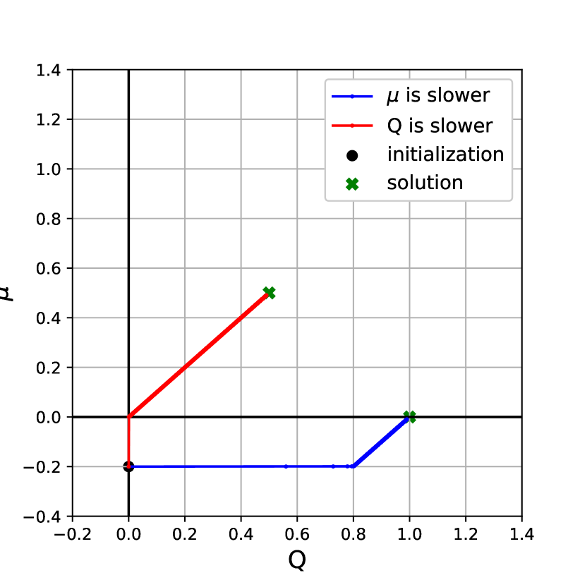
(a) $Q_{0}=0,\mu_{0}=-0.2$

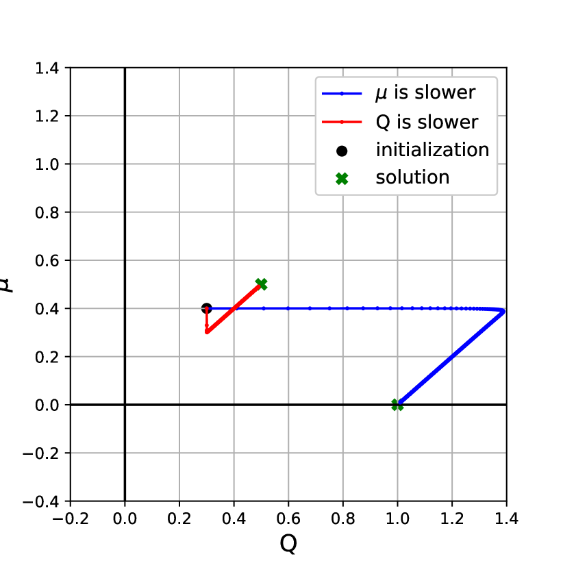
(b) $Q_{0}=0.3,\mu_{0}=0.4$

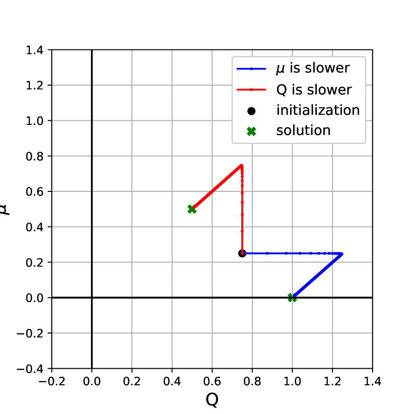
(c) $Q_{0}=0.75,\mu_{0}=0.25$

Figure 2: Visualization of $(Q,\mu)$ trajectories in the two-timescale algorithm: The learning rates are set as $\rho^{Q}=1,\rho^{\mu}=0.001$ so that $\mu$ runs slower than $Q$, and the learning rates are $\rho^{Q}=0.001,\rho^{\mu}=1$ so that $Q$ runs slower than $\mu$.

5 Unified convergence analysis

In this section, we provide a unified convergence analysis of the two-timescale Q-learning algorithm (4.1) for fixed learning rates $\rho^{Q},\rho^{\mu}>0$ covering all ratios $\rho^{Q}/\rho^{\mu}\in(0,\infty)$.

Our approach for establish unified convergence relies on the following Lyapunov function, inspired by the idea of Zhou and Lu (2023) for the analysis of single-timescale actor-critic method for the linear quadratic regulator problem. The Lyapunov function that we consider is

$$\mathcal{L}_{k}:=\mathcal{L}(\mu_{k},Q_{h,k})=W\|Q_{h,k}-Q_{h}^{*}\|_{\infty}+\|\mu_{k}-\tilde{\mu}_{k}\|_{\text{TV}},$$ (5.1)

where $Q_{h,k},\mu_{k}$ are numerical updates from the two-timescale Q-learning algorithm (4.1), $Q_{h}^{*}$ is the fixed point solving the Bellman equation

$$Q_{h}^{*}(x,a)=hf(x,a,\tilde{\mu}^{*})+e^{-\gamma h}\sum_{x^{\prime}}p(x^{\prime}\mid x,a,\tilde{\mu}^{*})\min_{a^{\prime}}Q_{h}^{*}(x^{\prime},a^{\prime}),$$ (5.2)

coupled with

$$\tilde{\mu}^{*}(x)=\tilde{\mu}^{*}P^{Q_{h}^{*},\tilde{\mu}^{*}}(x).$$ (5.3)

Here, we abuse the notations $Q_{h}^{*},\tilde{\mu}^{*}$ to represent fixed points, and they are independent from previous sections. Moreover, $\tilde{\mu}_{k}$ is an intermediate equilibrium distribution corresponding to each $Q_{h,k}$ so that

$$\tilde{\mu}_{k}=\tilde{\mu}_{k}P^{Q_{h,k},\tilde{\mu}_{k}}.$$ (5.4)

The weight parameter $W>0$ is to balance two discrepancies in (5.1), it will actually be chosen depending on the ratio $\rho^{Q}/\rho^{\mu}$. One cannot consider the Q-function update and the distribution update separately, since the operators $\mathcal{P}(Q,\mu)$ and $\mathcal{T}(Q,\mu)$ are highly coupled. Therefore, we devise such a Lyapunov function (5.1) in order to capture the global convergence of $Q$ functions and local convergence of $\mu$ at the same time. We will establish contraction of the Lyapunov function $\mathcal{L}_{k}$ following the algorithm (4.1).

5.1 Assumptions and main result

For our main result, we need following technical assumptions, which are standard and appear often in the analysis of convergence of Markov processes, see e.g., books like Meyn and Tweedie (2012).

Assumption 4

There exist $0<L_{p}<1,~{}L_{Q}>0$ such that for all $x\in\mathcal{X},\mu_{1},\mu_{2}\in\mathcal{P}(\mathcal{X}),Q_{1},Q_{2}$, we have the Lipschitz continuity

$$\sum_{x^{\prime}\in\mathcal{X}}\big{|}P^{Q_{1},\mu_{1}}(x,x^{\prime})-P^{Q_{2},\mu_{2}}(x,x^{\prime})\big{|}\leq L_{p}\|\mu_{1}-\mu_{2}\|_{\text{TV}}+L_{Q}\|Q_{1}-Q_{2}\|_{\infty}.$$

Assumption 5

(Uniform Doeblin’s condition) We assume that for any bounded $Q$, the transition probability $P^{Q,\mu}(x,x^{\prime})=p(x^{\prime}\mid x,\operatorname*{arg\,min}_{a}Q(x,a),\mu)$ has an equilibrium probability measure $\pi$ that solves $\pi=\pi P^{Q,\pi}$. There exist a constant

$$\beta\in\Big{(}\frac{1+L_{p}}{2},1\Big{)}$$

and probability measure $\nu$ such that

$$P^{Q,\pi}(x,\cdot)\geq\beta\nu(\cdot),$$ (5.5)

for all $x\in\mathcal{X}$.

Proposition 6

With Assumptions 4 and 5, for a fixed $Q_{h,k}$, there exists a unique equilibrium distribution solving (5.4). In addition with Assumptions 1, with sufficiently small $h$ and large $\gamma$ such that $\gamma h\gg 1$, there exists a unique fixed point $(Q_{h}^{*},\tilde{\mu}^{*})$ solving (5.2) and (5.3).

We defer the proof of the Proposition after Lemma 10.

Equipped with assumptions above, we are ready to state the main result: the unified convergence of (4.1).

Theorem 5.1

With Assumptions 1, 4, and 5, we require learning rates to satisfy that

$$0<\rho^{\mu}<2\beta-1-L_{p},\quad 0<\rho^{Q}<\frac{1}{1-e^{-\gamma h}}.$$ (5.6)

With these bounds, and taking $\Lambda_{\mu}=1-\rho^{\mu}\big{(}2\beta-1-L_{p}\big{)}$, the Lyapunov function (5.1) under the two-timescale Q-learning algorithm (4.1) contracts as

$$\mathcal{L}_{k}\leq(1-c)^{k}\mathcal{L}_{0}+\frac{2h\Lambda_{\mu}L_{Q}\rho^{Q}\|f\|_{\infty}}{c(1-e^{-\gamma h})(2\beta-1-L_{p})},$$ (5.7)

where $c=\min\{c_{1},c_{2}\}$ with

$$c_{1}=\rho^{Q}\Big{(}1-e^{-\gamma h}-\Big{(}L_{f}+\frac{L_{p}\|f\|_{\infty}}{e^{\gamma h}-1}\Big{)}\frac{hL_{Q}}{2\beta-1-L_{p}}\Big{)}-\frac{2\Lambda_{\mu}L_{Q}}{W(2\beta-1-L_{p})},$$ (5.8)

$$c_{2}=1-\Lambda_{\mu}-W\rho^{Q}h\big{(}L_{f}+\frac{L_{p}\|f\|_{\infty}}{e^{\gamma h}-1}\big{)}.$$

As $k\to\infty$, we have that $\mathcal{L}_{\infty}=O(\rho^{Q})$.

Our convergence result significantly extends that of Angiuli et al. (2023), which only considered extreme regimes where $\lim_{k\to\infty}\rho_{k}^{Q}/\rho_{k}^{\mu}=0$ and $\lim_{k\to\infty}\rho_{k}^{Q}/\rho_{k}^{\mu}=\infty$, and applied convergence results from Borkar (1997) directly with no quantitative convergence rates. Here we choose $\rho_{k}^{\mu},\rho_{k}^{Q}$ to be fixed constants $\rho^{\mu},\rho^{Q}$ rather than of the Robbins-Monro type as in Borkar (1997) for simplicity. We believe our result can be extended to Robbins-Monro type learning rates as well with some modifications.

Remark 7

Our quantitative convergence result sheds insight on how the contraction rate $1-c$ depends on learning rates $\rho^{Q},\rho^{\mu}$ precisely. The choices of $c$ in (5.7) illustrate the dichotomy convergence behaviors of the two-timescale Q-learning algorithm (4.1) when $\rho^{Q}\gg\rho^{\mu}$ or $\rho^{Q}\ll\rho^{\mu}$, thus get connected to MFG and MFC regimes.

• In the MFG regime where $\rho^{Q}\gg\rho^{\mu}$, recall $\Lambda_{\mu}=1-\rho^{\mu}\big{(}2\beta-1-L_{p}\big{)}$, we need to ensure

  $$c_{2}=\rho^{\mu}\big{(}2\beta-1-L_{p}\big{)}-W\rho^{Q}h\big{(}L_{f}+\frac{L_{p}\|f\|_{\infty}}{e^{\gamma h}-1}\big{)}>0,$$ (5.9)

  which implies that

  $$W<\frac{\rho^{\mu}\big{(}2\beta-1-L_{p}\big{)}}{\rho^{Q}h\big{(}L_{f}+\frac{L_{p}\|f\|_{\infty}}{e^{\gamma h}-1}\big{)}}\ll 1.$$ (5.10)

  It means that the convergence of $\mu$ dominates the convergence of (4.1), which is aligned with the fact that we have fast convergence for $Q$ and slow convergence for $\mu$.

• In the MFC regime where $\rho^{Q}\ll\rho^{\mu}$, we need to ensure $c_{1}>0$ so that

  $$W >\frac{2\Lambda_{\mu}L_{Q}}{\rho^{Q}(2\beta-1-L_{p})\Big{(}1-e^{-\gamma h}-\Big{(}L_{f}+\frac{L_{p}\|f\|_{\infty}}{e^{\gamma h}-1}\Big{)}\frac{hL_{Q}}{2\beta-1-L_{p}}\Big{)}}.$$ (5.11)

  It means that for sufficiently small $\rho^{Q}$, we need to put a larger weight on $Q$ convergence so that $Q$ dominates the whole process. It is aligned with our observation that in the MFC regime, we have fast convergence for $\mu$ and slow convergence for $Q$.

5.2 Auxiliary results

We first present some auxiliary results before proving Theorem 5.1. The following theorem investigates the case when $Q_{h,k}\equiv Q$ is fixed.

Proposition 8

Let $\mu_{k}$ update as in (4.1) with $Q_{h,k}\equiv Q$. Suppose $\tilde{\mu}$ is the equilibrium probability measure such that $\tilde{\mu}=\tilde{\mu}P^{Q,\tilde{\mu}}$, the transition probability satisfies Assumption 4, then given a fixed step size $\rho^{\mu}$ that satisfies

$$0<\rho^{\mu}<2\beta-1-L_{p}$$ (5.12)

and $\beta$ provided in Assumption 5, we can find a contraction rate $\Lambda_{\mu}=1-\rho^{\mu}\big{(}2\beta-1-L_{p}\big{)}$ such that for all $k\geq 0$,

$$\|\mu_{k+1}-\tilde{\mu}\|_{\text{TV}}\leq\Lambda_{\mu}\|\mu_{k}-\tilde{\mu}\|_{\text{TV}}.$$ (5.13)

Proof  The $\mu_{k}$ update step in (4.1) gives that

$$\mu_{k+1}-\tilde{\mu} =\mu_{k}-\tilde{\mu}+\rho^{\mu}\big{(}\mu_{k}P^{Q,\mu_{k}}-\mu_{k}\big{)}$$ (5.14)

$$=\mu_{k}-\tilde{\mu}+\rho^{\mu}\big{(}(\mu_{k}-\tilde{\mu})P^{Q,\tilde{\mu}}+\mu_{k}(P^{Q,\mu_{k}}-P^{Q,\tilde{\mu}})-(\mu_{k}-\tilde{\mu})\big{)}$$

$$=(1-\rho^{\mu})(\mu_{k}-\tilde{\mu})+\rho^{\mu}\big{(}(\mu_{k}-\tilde{\mu})P^{Q,\tilde{\mu}}+\mu_{k}(P^{Q,\mu_{k}}-P^{Q,\tilde{\mu}})\big{)}.$$

Using the triangle inequality, we have that

$$\|\mu_{k+1}-\tilde{\mu}\|_{\text{TV}} \leq(1-\rho^{\mu})\|\mu_{k}-\tilde{\mu}\|_{\text{TV}}+\rho^{\mu}\|(\mu_{k}-\tilde{\mu})P^{Q,\tilde{\mu}}\|_{\text{TV}}$$ (5.15)

$$\quad+\rho^{\mu}\|\mu_{k}(P^{Q,\mu_{k}}-P^{Q,\tilde{\mu}})\|_{\text{TV}}=(1-\rho^{\mu})\|\mu_{k}-\tilde{\mu}\|_{\text{TV}}+I+II.$$

To treat $I$, we decompose $\mu_{k}-\tilde{\mu}$ as

$$\mu_{k}-\tilde{\mu}=(\mu_{k}-\tilde{\mu})_{+}-(\mu_{k}-\tilde{\mu})_{-}=:S_{+}-S_{-}.$$ (5.16)

Note that for any $A\subseteq\mathcal{X}$, by (5.5),

$$\sum_{x\in A}\sum_{x_{0}\in\mathcal{X}}S_{\pm}(x_{0})P^{Q,\tilde{\mu}}(x_{0},x)\geq\beta\sum_{x\in A}\sum_{x_{0}\in\mathcal{X}}S_{\pm}(x_{0})\nu(x),$$ (5.17)

and

$$\sum_{x\in A}\sum_{x_{0}\in\mathcal{X}}S_{+}(x_{0})\nu(x)=\sum_{x\in A}\sum_{x_{0}\in\mathcal{X}}S_{-}(x_{0})\nu(x).$$ (5.18)

Therefore, we use (5.18) and apply the triangle inequality to get

$$\|(\mu_{k}-\tilde{\mu})P^{Q,\tilde{\mu}}\|_{\text{TV}}=\sup_{A\subseteq\mathcal{X}}\Big{|}\sum_{x\in A}S_{+}P^{Q,\tilde{\mu}}(x)-S_{-}P^{Q,\tilde{\mu}}(x)\Big{|}$$ (5.19)

$$\leq\sup_{A\subseteq\mathcal{X}}\Big{|}\sum_{x\in A}S_{+}P^{Q,\tilde{\mu}}(x)-\beta\sum_{x\in A}\sum_{x_{0}\in\mathcal{X}}S_{+}(x_{0})\nu(x)\Big{|}+\sup_{A\subseteq\mathcal{X}}\Big{|}\sum_{x\in A}S_{-}P^{Q,\tilde{\mu}}(x)-\beta\sum_{x\in A}\sum_{x_{0}\in\mathcal{X}}S_{-}(x_{0})\nu(x)\Big{|}$$

$$=\sum_{x\in\mathcal{X}}\Big{(}S_{+}P^{Q,\tilde{\mu}}(x)-\beta\sum_{x_{0}\in\mathcal{X}}S_{+}(x_{0})\nu(x)\Big{)}+\sum_{x\in\mathcal{X}}\Big{(}S_{-}P^{Q,\tilde{\mu}}(x)-\beta\sum_{x_{0}\in\mathcal{X}}S_{-}(x_{0})\nu(x)\Big{)}$$

$$=\sum_{x\in\mathcal{X}}\sum_{x_{0}\in\mathcal{X}}(S_{+}+S_{-})(x_{0})P^{Q,\tilde{\mu}}(x_{0},x)-\beta\sum_{x\in\mathcal{X}}\sum_{x_{0}\in\mathcal{X}}(S_{+}+S_{-})(x_{0})\nu(x)$$

$$=(1-\beta)\sum_{x_{0}\in\mathcal{X}}|\mu_{k}(x_{0})-\tilde{\mu}(x_{0})|=(1-\beta)\|\mu_{k}-\tilde{\mu}\|_{1}=2(1-\beta)\|\mu_{k}-\tilde{\mu}\|_{\text{TV}},$$

where the second equality above uses (5.17).

For $II$, we use Assumption 4 to get

$$\|\mu_{k}(P^{Q,\mu_{k}}-P^{Q,\tilde{\mu}})\|_{\text{TV}} =\sup_{A\subseteq\mathcal{X}}\Big{|}\sum_{x\in A}\sum_{x_{0}\in\mathcal{X}}\mu_{k}(x_{0})\big{(}P^{Q,\mu_{k}}(x_{0},x)-P^{Q,\tilde{\mu}}(x_{0},x)\big{)}\Big{|}$$ (5.20)

$$\leq\sum_{x\in\mathcal{X}}\sum_{x_{0}\in\mathcal{X}}\mu_{k}(x_{0})\Big{|}P^{Q,\mu_{k}}(x_{0},x)-P^{Q,\tilde{\mu}}(x_{0},x)\Big{|}$$

$$\leq L_{p}\|\mu_{k}-\tilde{\mu}\|_{\text{TV}}\sum_{x_{0}\in\mathcal{X}}\mu_{k}(x_{0})=L_{p}\|\mu_{k}-\tilde{\mu}\|_{\text{TV}}.$$

Combining all parts together, we have

$$\|\mu_{k+1}-\tilde{\mu}\|_{\text{TV}}\leq\Big{(}1-\rho^{\mu}\big{(}2\beta-1-L_{p}\big{)}\Big{)}\|\mu_{k}-\tilde{\mu}\|_{\text{TV}}.\hfill\rule{6.45831pt}{6.45831pt}$$

 

Now let $Q_{h,k}$ update as in the algorithm, we have the following iteration bound for $Q_{h,k}$.

Proposition 9

With Assumptions 1 and 4, we can find a contraction rate $\Lambda_{Q}=1-\rho^{Q}(1-e^{-\gamma h})\in(0,1)$ such that the maximal difference between $Q_{h,k}$ and the fixed point $Q_{h}^{*}$ in (5.2) iterates as

$$\|{Q}_{h,k+1}-Q_{h}^{*}\|_{\infty}\leq(1-\rho^{Q}(1-e^{-\gamma h}))\|{Q}_{h,k}-Q_{h}^{*}\|_{\infty}+\rho^{Q}h\|\mu_{k}-\tilde{\mu}^{*}\|_{\text{TV}}\Big{(}L_{f}+\frac{L_{p}}{e^{\gamma h}-1}\|f\|_{\infty}\Big{)}.$$ (5.21)

Proof  We rewrite the absolute value difference

$$\Delta_{k}(x,a):=|{Q}_{h,k}(x,a)-Q_{h}^{*}(x,a)|$$ (5.22)

for shortness. The two-timescale Q-learning (4.1) gives that

$$Q_{h,k+1} (x,a)-Q_{h}^{*}(x,a)=Q_{h,k}(x,a)-Q_{h}^{*}(x,a)+\rho^{Q}\mathcal{T}(Q_{h,k},\mu_{k})$$ (5.23)

$$=(1-\rho^{Q})(Q_{h,k}(x,a)-Q_{h}^{*}(x,a))+\rho^{Q}\Big{(}hf(x,a,\mu_{k})-hf(x,a,\tilde{\mu}^{*})$$

$$\quad+e^{-\gamma h}\sum_{x^{\prime}\in\mathcal{X}}p(x^{\prime}\mid x,a,\mu_{k})\inf_{a^{\prime}}Q_{h,k}(x^{\prime},a^{\prime})-e^{-\gamma h}\sum_{x^{\prime}\in\mathcal{X}}p(x^{\prime}\mid x,a,\tilde{\mu}^{*})\inf_{a^{\prime}}Q_{h}^{*}(x^{\prime},a^{\prime})\Big{)}.$$

By the triangle inequality, we get that

$$\Delta_{k+1}(x,a) \leq(1-\rho^{Q})\Delta_{k}(x,a)+\rho^{Q}h|f(x,a,\mu_{k})-f(x,a,\tilde{\mu}^{*})|$$ (5.24)

$$~{}~{}~{}+\rho^{Q}e^{-\gamma h}\Big{|}\sum_{x^{\prime}\in\mathcal{X}}p(x^{\prime}\mid x,a,\mu_{k})\inf_{a^{\prime}}Q_{h,k}(x^{\prime},a^{\prime})-\sum_{x^{\prime}\in\mathcal{X}}p(x^{\prime}\mid x,a,\tilde{\mu}^{*})\inf_{a^{\prime}}Q_{h}^{*}(x^{\prime},a^{\prime})\Big{|}$$

$$\leq(1-\rho^{Q})\Delta_{k}(x,a)+I+II+III,$$

where

$$I =\rho^{Q}h|f(x,a,\mu_{k})-f(x,a,\tilde{\mu}^{*})|,$$

$$II =\rho^{Q}e^{-\gamma h}\Big{|}\sum_{x^{\prime}\in\mathcal{X}}p(x^{\prime}\mid x,a,\mu_{k})\inf_{a^{\prime}}Q_{h,k}(x^{\prime},a^{\prime})-\sum_{x^{\prime}\in\mathcal{X}}p(x^{\prime}\mid x,a,\tilde{\mu}^{*})\inf_{a^{\prime}}Q_{h,k}(x^{\prime},a^{\prime})\Big{|},$$

$$III =\rho^{Q}e^{-\gamma h}\Big{|}\sum_{x^{\prime}\in\mathcal{X}}p(x^{\prime}\mid x,a,\tilde{\mu}^{*})\inf_{a^{\prime}}Q_{h,k}(x^{\prime},a^{\prime})-\sum_{x^{\prime}\in\mathcal{X}}p(x^{\prime}\mid x,a,\tilde{\mu}^{*})\inf_{a^{\prime}}Q_{h}^{*}(x^{\prime},a^{\prime})\Big{|}.$$

For $I$, we use the Assumption 1 to get

$$I\leq\rho^{Q}hL_{f}\|\mu_{k}-\tilde{\mu}^{*}\|_{\text{TV}}.$$ (5.25)

For $II$, we use the Assumption 4 to get

$$II\leq\rho^{Q}e^{-\gamma h}\|Q_{h,k}\|_{\infty}L_{p}\|\mu_{k}-\tilde{\mu}^{*}\|_{\text{TV}}\leq\rho^{Q}\frac{L_{p}h}{e^{\gamma h}-1}\|f\|_{\infty}\|\mu_{k}-\tilde{\mu}^{*}\|_{\text{TV}},$$ (5.26)

since by the definition of discrete time Q-function,

$$\|Q_{h,k}\|_{\infty}\leq\frac{h}{1-e^{-\gamma h}}\|f\|_{\infty}.$$ (5.27)

For $III$, we have

$$III\leq\rho^{Q}e^{-\gamma h}\sup_{a^{\prime}}\sup_{x^{\prime}\in\mathcal{X}}\Delta_{k}(x^{\prime},a^{\prime}).$$ (5.28)

Now combining all bounds of $I,II,III$ together, we can take the supremum over $(x,a)\in\mathcal{X}\times\mathcal{A}$ on the right side first and left side later to obtain that

$$\|{Q}_{h,k+1}-Q_{h}^{*}\|_{\infty}\leq(1-\rho^{Q}(1-e^{-\gamma h}))\|{Q}_{h,k}-Q_{h}^{*}\|_{\infty}+\rho^{Q}h\|\mu_{k}-\tilde{\mu}^{*}\|_{\text{TV}}\Big{(}L_{f}+\frac{L_{p}}{e^{\gamma h}-1}\|f\|_{\infty}\Big{)}.$$

 

We do not know the relation between $\tilde{\mu}_{k}$ and $\tilde{\mu}^{*}$ a priori, since the equation $\mu=\mu P^{Q,\mu}$ is highly nonlinear. However, we can control the difference between two equilibrium distributions by the difference of their corresponding $Q$-functions, if one of $P^{Q,\mu}$ satisfies the uniform Doeblin’s condition.

Lemma 10

Given $Q_{1},Q_{2}\in{\mathbb{R}}_{+}$, if $\mu_{1},\mu_{2}\in\mathcal{P}(\mathcal{X})$ solves

$$\mu_{1}(I-P^{Q_{1},\mu_{1}})=0,\quad\mu_{2}(I-P^{Q_{2},\mu_{2}})=0$$ (5.29)

respectively, then based on Assumptions 4 and 5 of $P^{Q_{2},\mu_{2}}$ (or $P^{Q_{1},\mu_{1}}$), we have the relation

$$\|\mu_{1}-\mu_{2}\|_{\text{TV}}\leq\frac{L_{Q}}{2\beta-1-L_{p}}\|Q_{1}-Q_{2}\|_{\infty}.$$ (5.30)

Proof  The proof resembles the proof of Proposition 8. Note that

$$\|\mu_{1}-\mu_{2}\|_{\text{TV}}=\|\mu_{1}P^{Q_{1},\mu_{1}}-\mu_{2}P^{Q_{2},\mu_{2}}\|_{\text{TV}}\leq\|(\mu_{1}-\mu_{2})P^{Q_{2},\mu_{2}}\|_{\text{TV}}+\|\mu_{1}\big{(}P^{Q_{1},\mu_{1}}-P^{Q_{2},\mu_{2}}\big{)}\|_{\text{TV}}.$$ (5.31)

The first term above can be treated in the same way as for part $I$ in (5.15) to have the bound

$$\|(\mu_{1}-\mu_{2})P^{Q_{2},\mu_{2}}\|_{\text{TV}}\leq 2(1-\beta)\|\mu_{1}-\mu_{2}\|_{\text{TV}}.$$ (5.32)

The second term in (5.31) uses Assumption 4 so that

$$\|\mu_{1}\big{(}P^{Q_{1},\mu_{1}}-P^{Q_{2},\mu_{2}}\big{)}\|_{\text{TV}}\leq L_{p}\|\mu_{1}-\mu_{2}\|_{\text{TV}}+L_{Q}\|Q_{1}-Q_{2}\|_{\infty}.$$ (5.33)

Combining all terms together we have

$$(2\beta-1-L_{p})\|\mu_{1}-\mu_{2}\|_{\text{TV}}\leq L_{Q}\|Q_{1}-Q_{2}\|_{\infty}$$ (5.34)

to obtain the relation.  
Based on Lemma 10, we can control the difference between $\tilde{\mu}_{k}$ and $\tilde{\mu}^{*}$ to be

$$\|\tilde{\mu}_{k}-\tilde{\mu}^{*}\|_{\text{TV}}\leq\frac{L_{Q}}{2\beta-1-L_{p}}\|Q_{h,k}-Q_{h}^{*}\|_{\infty}.$$ (5.35)

Proof [Proof of Proposition 6]Consider the mapping $\mathcal{M}_{Q}:\mathcal{P}(\mathcal{X})\to\mathcal{P}(\mathcal{X})$ such that $\mathcal{M}_{Q}(\mu)=\mu P^{Q,\mu}$. For a given $Q$, $\mathcal{M}_{Q}$ is continuous since

$$\|\mathcal{M}_{Q}(\mu_{1})-\mathcal{M}_{Q}(\mu_{2})\|_{\text{TV}} =\|\mu_{1}P^{Q,\mu_{1}}-\mu_{2}P^{Q,\mu_{2}}\|_{\text{TV}}$$ (5.36)

$$\leq\|(\mu_{1}-\mu_{2})P^{Q,\mu_{1}}\|_{\text{TV}}+\|\mu_{2}(P^{Q,\mu_{1}}-P^{Q,\mu_{2}})\|_{\text{TV}}$$

$$\leq 2(1-\beta)\|\mu_{1}-\mu_{2}\|_{\text{TV}}+L_{p}\|\mu_{1}-\mu_{2}\|_{\text{TV}}$$

$$=(2(1-\beta)+L_{p})\|\mu_{1}-\mu_{2}\|_{\text{TV}}.$$

Because $\mathcal{X}$ is finite, by Brouwer’s fixed point theorem, there exists $\mu$ such that $\mathcal{M}_{Q}(\mu)=\mu$ for the given $Q$. This fixed point $\mu$ is unique due to (5.34).

For equations (5.2) and (5.3), we define the Bellman operator

$$\mathcal{B}_{\mu}(Q)(x,a):=hf(x,a,\mu)+e^{-\gamma h}\sum_{x^{\prime}}p(x^{\prime}\mid x,a,\mu)\min_{a^{\prime}}Q(x^{\prime},a^{\prime}).$$ (5.37)

The mapping pair $(\mathcal{B}_{\mu}(Q),\mathcal{M}_{Q}(\mu)):{\mathbb{R}}_{+}\times\mathcal{P}(\mathcal{X})\to{\mathbb{R}}_{+}\times\mathcal{P}(\mathcal{X})$ is continuous since

$$\|\mathcal{B}_{\mu_{1}}(Q_{1})-\mathcal{B}_{\mu_{2}}(Q_{2})\|_{\infty} \leq\|\mathcal{B}_{\mu_{1}}(Q_{1})-\mathcal{B}_{\mu_{2}}(Q_{1})\|_{\infty}+\|\mathcal{B}_{\mu_{2}}(Q_{1})-\mathcal{B}_{\mu_{2}}(Q_{2})\|_{\infty}$$ (5.38)

$$\leq(hL_{f}+e^{-\gamma h}L_{p}\|Q\|_{\infty})\|\mu_{1}-\mu_{2}\|_{\text{TV}}+e^{-\gamma h}\|Q_{1}-Q_{2}\|_{\infty},$$

and

$$\|\mathcal{M}_{Q_{1}}(\mu_{1})-\mathcal{M}_{Q_{2}}(\mu_{2})\|_{\text{TV}} \leq\|\mathcal{M}_{Q_{1}}(\mu_{1})-\mathcal{M}_{Q_{2}}(\mu_{1})\|_{\text{TV}}+\|\mathcal{M}_{Q_{2}}(\mu_{1})-\mathcal{M}_{Q_{2}}(\mu_{2})\|_{\text{TV}}$$ (5.39)

$$\leq L_{Q}\|Q_{1}-Q_{2}\|_{\infty}+(2(1-\beta)+L_{p})\|\mu_{1}-\mu_{2}\|_{\text{TV}}.$$

Thus by Brouwer’s fixed point theorem, there exists a fixed point $(Q_{h}^{*},\tilde{\mu}^{*})$ solving (5.2) and (5.3). In terms of uniqueness, suppose that we have two fixed points $(Q_{h,1}^{*},\tilde{\mu}_{1}^{*})$ and $(Q_{h,2}^{*},\tilde{\mu}_{2}^{*})$ both solving (5.2) and (5.3), by Lemma 10, we have

$$\|\tilde{\mu}_{1}^{*}-\tilde{\mu}_{2}^{*}\|_{\text{TV}}\leq\frac{L_{Q}}{2\beta-1-L_{p}}\|Q_{h,1}^{*}-Q_{h,2}^{*}\|_{\infty}.$$ (5.40)

On the other hand,

$$\|Q_{h,1}^{*}-Q_{h,2}^{*}\|_{\infty} =\|\mathcal{B}_{\tilde{\mu}_{1}^{*}}(Q_{h,1}^{*})-\mathcal{B}_{\tilde{\mu}_{2}^{*}}(Q_{h,1}^{*})\|_{\infty}$$ (5.41)

$$\leq(hL_{f}+e^{-\gamma h}L_{p}\|Q\|_{\infty})\|\tilde{\mu}_{1}^{*}-\tilde{\mu}_{2}^{*}\|_{\text{TV}}+e^{-\gamma h}\|Q_{h,1}^{*}-Q_{h,2}^{*}\|_{\infty},$$

so that

$$\|\tilde{\mu}_{1}^{*}-\tilde{\mu}_{2}^{*}\|_{\text{TV}}\leq\frac{L_{Q}}{2\beta-1-L_{p}}\frac{hL_{f}+e^{-\gamma h}L_{p}\|Q\|_{\infty}}{1-e^{-\gamma h}}\|\tilde{\mu}_{1}^{*}-\tilde{\mu}_{2}^{*}\|_{\text{TV}}.$$ (5.42)

With sufficiently small $h$ and large $\gamma$ such that $\gamma h\gg 1$, we have the factor

$$\frac{L_{Q}}{2\beta-1-L_{p}}\frac{hL_{f}+e^{-\gamma h}L_{p}\|Q\|_{\infty}}{1-e^{-\gamma h}}<1,$$ (5.43)

and therefore $\tilde{\mu}_{1}^{*}=\tilde{\mu}_{2}^{*}$ in the total variation norm, which implies that $Q_{h,1}^{*}=Q_{h,2}^{*}$.  

5.3 Proof of Theorem 5.1

Proof  The proof strategy is to obtain the iteration inequality in the form

$$\mathcal{L}_{k+1}-\mathcal{L}_{k} =W\|Q_{h,k+1}-Q_{h}^{*}\|_{\infty}-W\|Q_{h,k}-Q_{h}^{*}\|_{\infty}+\|\mu_{k+1}-\tilde{\mu}_{k+1}\|_{\text{TV}}-\|\mu_{k}-\tilde{\mu}_{k}\|_{\text{TV}}$$

$$\leq-c\mathcal{L}_{k}+e_{k},$$

with some $c\in(0,1)$ and bounded errors $e_{k}$. Then by iteration, we can get that for each $k\geq 1$,

$$\mathcal{L}_{k}\leq(1-c)^{k}\mathcal{L}_{0}+\sum_{j=0}^{k-1}(1-c)^{k-1-j}e_{j}.$$ (5.44)

Estimate on $\mu_{k}-\tilde{\mu}_{k}$

The proof of Proposition 8 implies that

$$\|\mu_{k+1}-\tilde{\mu}_{k+1}\|_{\text{TV}}\leq\Lambda_{\mu}\|\mu_{k}-\tilde{\mu}_{k+1}\|_{\text{TV}}.$$ (5.45)

Therefore, in addition with the triangle inequality, we can write

$$\|\mu_{k+1} -\tilde{\mu}_{k+1}\|_{\text{TV}}-\|\mu_{k}-\tilde{\mu}_{k}\|_{\text{TV}}\leq\Lambda_{\mu}\|\mu_{k}-\tilde{\mu}_{k+1}\|_{\text{TV}}-\|\mu_{k}-\tilde{\mu}_{k}\|_{\text{TV}}$$ (5.46)

$$\leq\Lambda_{\mu}\|\tilde{\mu}_{k+1}-\tilde{\mu}_{k}\|_{\text{TV}}-(1-\Lambda_{\mu})\|\mu_{k}-\tilde{\mu}_{k}\|_{\text{TV}}$$

$$\leq\Lambda_{\mu}\big{(}\|\tilde{\mu}_{k}-\tilde{\mu}^{*}\|_{\text{TV}}+\|\tilde{\mu}_{k+1}-\tilde{\mu}^{*}\|_{\text{TV}}\big{)}-(1-\Lambda_{\mu})\|\mu_{k}-\tilde{\mu}_{k}\|_{\text{TV}}$$

$$\leq\frac{\Lambda_{\mu}L_{Q}}{2\beta-1-L_{p}}\Big{(}\|Q_{h,k}-Q_{h}^{*}\|_{\infty}+\|Q_{h,k+1}-Q_{h}^{*}\|_{\infty}\Big{)}-(1-\Lambda_{\mu})\|\mu_{k}-\tilde{\mu}_{k}\|_{\text{TV}}$$

$$\leq\frac{2\Lambda_{\mu}L_{Q}}{2\beta-1-L_{p}}\|Q_{h,k}-Q_{h}^{*}\|_{\infty}+\frac{\Lambda_{\mu}L_{Q}\rho^{Q}}{2\beta-1-L_{p}}\|\mathcal{T}(\cdot,\cdot)\|_{\infty}-(1-\Lambda_{\mu})\|\mu_{k}-\tilde{\mu}_{k}\|_{\text{TV}},$$

where the last inequality is obtained by the Q iteration in (4.1) and the uniform boundedness of the operator $\mathcal{T}$ over $Q,\mu$.

Estimate on $Q_{h,k}-Q_{h}^{*}$

Based on Proposition 9, we have that

$$\|Q_{h,k+1}-Q_{h}^{*}\|_{\infty}-\|Q_{h,k}-Q_{h}^{*}\|_{\infty}$$ (5.47)

$$\leq-\rho^{Q}(1-e^{-\gamma h})\|Q_{h,k}-Q_{h}^{*}\|_{\infty}+\rho^{Q}h\Big{(}L_{f}+\frac{L_{p}}{e^{\gamma h}-1}\|f\|_{\infty}\Big{)}\|\mu_{k}-\tilde{\mu}^{*}\|_{\text{TV}}$$

$$\leq-\rho^{Q}(1-e^{-\gamma h})\|Q_{h,k}-Q_{h}^{*}\|_{\infty}+\rho^{Q}h\Big{(}L_{f}+\frac{L_{p}}{e^{\gamma h}-1}\|f\|_{\infty}\Big{)}\Big{(}\|\mu_{k}-\tilde{\mu}_{k}\|_{\text{TV}}+\|\tilde{\mu}_{k}-\tilde{\mu}^{*}\|_{\text{TV}}\Big{)}$$

$$\leq-\rho^{Q}(1-e^{-\gamma h})\|Q_{h,k}-Q_{h}^{*}\|_{\infty}$$

$$\quad+\rho^{Q}h\Big{(}L_{f}+\frac{L_{p}}{e^{\gamma h}-1}\|f\|_{\infty}\Big{)}\Big{(}\|\mu_{k}-\tilde{\mu}_{k}\|_{\text{TV}}+\frac{L_{Q}}{2\beta-1-L_{p}}\|Q_{h,k}-Q_{h}^{*}\|_{\infty}\Big{)},$$

where in the last inequality we use (5.35).

Combined estimates

Now we are ready to combine (5.46) and (5.47) together and obtain that

$$\mathcal{L}_{k+1}-\mathcal{L}_{k}$$

$$\leq\Big{(}-W\rho^{Q}(1-e^{-\gamma h})+W\rho^{Q}h\Big{(}L_{f}+\frac{L_{p}\|f\|_{\infty}}{e^{\gamma h}-1}\Big{)}\frac{L_{Q}}{2\beta-1-L_{p}}+\frac{2\Lambda_{\mu}L_{Q}}{2\beta-1-L_{p}}\Big{)}\|Q_{h,k}-Q_{h}^{*}\|_{\infty}$$

$$\quad-\Big{(}1-\Lambda_{\mu}-W\rho^{Q}h\Big{(}L_{f}+\frac{L_{p}\|f\|_{\infty}}{e^{\gamma h}-1}\Big{)}\Big{)}\|\mu_{k}-\tilde{\mu}_{k}\|_{\text{TV}}+\frac{\Lambda_{\mu}L_{Q}\rho^{Q}}{2\beta-1-L_{p}}\|\mathcal{T}(\cdot,\cdot)\|_{\infty}$$

$$\leq-c\mathcal{L}_{k}+e_{k}.$$

This inequality holds if we let

$$c_{1}:=\rho^{Q}\Big{(}1-e^{-\gamma h}-\Big{(}L_{f}+\frac{L_{p}\|f\|_{\infty}}{e^{\gamma h}-1}\Big{)}\frac{hL_{Q}}{2\beta-1-L_{p}}\Big{)}-\frac{2\Lambda_{\mu}L_{Q}}{W(2\beta-1-L_{p})},$$ (5.48)

$$c_{2}:=1-\Lambda_{\mu}-W\rho^{Q}h\big{(}L_{f}+\frac{L_{p}\|f\|_{\infty}}{e^{\gamma h}-1}\big{)},$$

and we require that

$$c:=\min\{c_{1},c_{2}\}\in(0,1),$$ (5.49)

with the error term denoted as

$$e_{k}:=\frac{\Lambda_{\mu}L_{Q}\rho^{Q}}{2\beta-1-L_{p}}\|\mathcal{T}(\cdot,\cdot)\|_{\infty}.$$ (5.50)

Note that by (4.1) and (5.27), $\|\mathcal{T}(\cdot,\cdot)\|_{\infty}$ is bounded by

$$\|\mathcal{T}(\cdot,\cdot)\|_{\infty}\leq h\|f\|_{\infty}+(e^{-\gamma h}+1)\|Q_{h,k}\|_{\infty}\leq\frac{2h}{1-e^{-\gamma h}}\|f\|_{\infty}.$$ (5.51)

Eventually we have the convergence

$$\mathcal{L}_{k} \leq(1-c)^{k}\mathcal{L}_{0}+\frac{2h\Lambda_{\mu}L_{Q}\rho^{Q}\|f\|_{\infty}}{(1-e^{-\gamma h})(2\beta-1-L_{p})}\sum_{j=0}^{k-1}(1-c)^{k-1-j}$$

$$\leq(1-c)^{k}\mathcal{L}_{0}+\frac{2h\Lambda_{\mu}L_{Q}\rho^{Q}\|f\|_{\infty}}{c(1-e^{-\gamma h})(2\beta-1-L_{p})}.$$

 

6 Numerical experiment

We carry out some numerical experiments to validate our convergence result of (4.1) with different ratios of fixed learning rates $\rho^{\mu}$ and $\rho^{Q}$. Our examples are adapted from those of Angiuli et al. (2022) with slight modifications. The algorithm we use is sample-based with stochastic approximations to the iterations (4.1). For better control of the numerical comparison, we use the maximum number of iterations $N_{k}$ as stopping criterion.

Algorithm 1 Unified Two-timescales Q-learning - Tabular version

0:  $T$ : number of time steps in a learning episode, $\mathcal{{X}}=\{x_{0},\dots,x_{|\mathcal{{X}}|-1}\}$ : finite state space. $\mathcal{{A}}=\{a_{0},\dots,a_{|\mathcal{{A}}|-1}\}$ : finite action space. $\mu_{0}$ : initial distribution of the representative player.$\epsilon$ : parameter related to the $\epsilon$-greedy policy.$N_{k}$ : number of episodes.$\gamma,h:$ fixed constants.

1:  Initialization: $Q^{0}(x,a)=0$ for all $(x,a)\in\mathcal{{X}}\times\mathcal{{A}}$, $\mu^{0}_{n}=\left(\frac{1}{|\mathcal{{X}}|},\dots,\frac{1}{|\mathcal{{X}}|}\right)$ for $n=0,\dots,T$

2:  for each episode $k=1,2,\dots N_{k}$ do

3:     Initialization: Sample $X^{k}_{0}\sim\mu^{k-1}_{T}$ and set $Q^{k}\equiv Q^{k-1}$

4:     for $n\leftarrow 0$ to $T-1$ do

5:        Update $\mu$: $\mu^{k}_{n}=\mu^{k-1}_{n}+\rho^{\mu}(\bm{\delta}(X^{k}_{n})-\mu^{k-1}_{n})$ where $\bm{\delta}(X^{k}_{n})=\left(\mathbf{1}_{x_{0}}(X^{k}_{n}),\dots,\mathbf{1}_{x_{|\mathcal{X}|-1}}(X^{k}_{n})\right)$

6:        Choose action $A^{k}_{n}$ using the $\epsilon$-greedy policy derived from $Q^{k}(X^{k}_{n},\cdot)$ Observe cost $f_{n+1}=f(X^{k}_{n},A^{k}_{n},\mu^{k}_{n})$ and state $X^{k}_{n+1}$ provided by the environment

7:        Update $Q$:$Q^{k}(X^{k}_{n},A^{k}_{n})=Q^{k}(X^{k}_{n},A^{k}_{n})+\rho^{Q}[hf_{n+1}+e^{-\gamma h}\min_{a^{\prime}\in\mathcal{A}}Q^{k}(X^{k}_{n+1},a^{\prime})-Q^{k}(X^{k}_{n},A^{k}_{n})]$

8:     end for

9:  end for

10:  return  $(\mu^{k},Q^{k})$

Benchmark problem

For MFG and MFC problems introduced in (2.4) and (2.5), we take $\mathcal{X},\mathcal{A}\subset\mathbb{R}$, and define the cost function

$$f(x,\alpha,\mu)=\frac{1}{2}\alpha^{2}+c_{1}\left(x-c_{2}m\right)^{2}+c_{3}\left(x-c_{4}\right)^{2}+c_{5}m^{2},\qquad b(x,\alpha,\mu)=\alpha,$$ (6.1)

where $m=\sum_{x\in\mathcal{X}}x\mu(x)$, $c_{1}=0.25$, $c_{2}=1.5$, $c_{3}=0.50$, $c_{4}=0.6$, $c_{5}=5$, discount parameter $\gamma=1$ and volatility $\sigma=0.3$. The infinite time horizon is truncated at time $T=20$. The continuous time is discretized using step $h=0.01$. We adopt a larger action space $\mathcal{A}=\{a_{0}=-2,\dots,a_{N_{\mathcal{A}}}=2\}$ and the state space is $\mathcal{X}=\{x_{0}=-2+x_{c},\dots,x_{N_{\mathcal{X}}}=2+x_{c}\}$, where $x_{c}$ is the center of the state space. The step size for the discretization of the state and action spaces $\mathcal{X}$ and $\mathcal{A}$ is given by $\Delta=\sqrt{h}=0.1$. For the discretization of the SDE $dX_{t}=\alpha_{t}dt+\sigma dB_{t}$, we consider the transition matrix given by

$$p(x^{\prime}\mid x,a,\mu)\propto\mathbb{P}(Z\in[x^{\prime}-\Delta/2,x^{\prime}+\Delta/2])$$ (6.2)

with $Z\sim\mathcal{N}(x+a,\sigma^{2}h)$; the distribution is normalized to avoid any artifacts due to numerical approximations.

We use the unified two timescale mean field Q-learning algorithm in Angiuli et al. (2022) with a fixed ratio of step sizes $\rho^{Q}$ and $\rho^{\mu}$. In the Q-learning, we set the number of episodes $N_{k}=140000$ and the learning rates $\rho^{Q}=0.02,\rho^{\mu}=0.0001$ (and hence ratio $\rho^{Q}/\rho^{\mu}=200$) for the MFG problem, $\rho^{Q}=0.0001,\rho^{\mu}=0.5$ (ratio $\rho^{Q}/\rho^{\mu}=0.0002$) for the MFC problem.

Results

We compare the numerical value functions achieved by the two-timescale Q-learning algorithm with the calculated theoretical value functions: Figure 3(a) plots value functions of MFG and Figure 3(b) plots value functions of MFC problem. One can calculate theoretical value functions from the HJB equations based on Theorem 2, and we refer computation details to (Angiuli et al., 2022, Appendix A). In addition, we present the optimal control function $\hat{\alpha}=\arg\min_{a}Q(x,a)$ and the theoretical optimal control function in Figure 3(c) for MFG and in Figure 3(d) for MFC problem. Figure 3(e) shows the empirical equilibrium distribution averaged over last $10000$ episodes in the unified two-timescale Q-learning algorithm with different ratios of learning rates $\rho^{\mu},\rho^{Q}$.

(a) MFG Value function

(b) MFC Value function

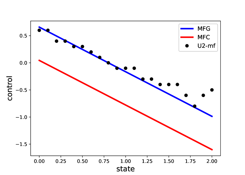
(c) MFG control averaged over last 10000 episodes

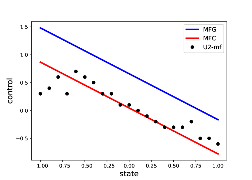
(d) MFC control averaged over last 10000 episodes

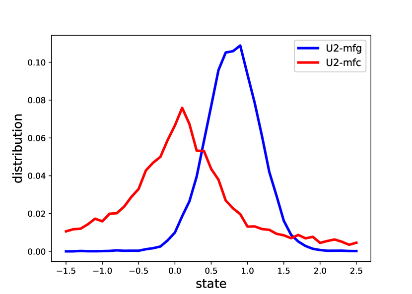
(e) MFG and MFC distribution averaged over last 10000 episodes

Figure 3: Numerical results of the two-timescale Q-learning algorithm where MFG learning rates are $\rho^{Q}=0.02,\rho^{\mu}=0.0001$, and MFC learning rates are $\rho^{Q}=0.0001,\rho^{\mu}=0.5$. The theoretical value/control functions are represented by solid lines and numerical value/control functions are represented by dotted lines in figure 3(a)-3(d).

Intermediate ratios of $\rho^{Q}/\rho^{\mu}$

In addition to extreme ratios where numerically $\rho^{Q}/\rho^{\mu}=200$ for MFG problem and $\rho^{Q}/\rho^{\mu}=0.0002$ for MFC problem, we take some intermediate ratios where $\rho^{Q}/\rho^{\mu}=10,1,0.1$ and present the respective resulting value functions in Figure 4. In the figure, the theoretical solutions are labeled “MFG” and “MFC” and represented by solid lines, and the numerical results of two timescale algorithm are labeled with prefix “U2-” and represented by dotted lines. We observe in the intermediate regimes, the algorithms seem to converge to some solutions lying between the MFG and MFC value functions; while in this work we do not identify these limits, this would be an interesting future research direction.

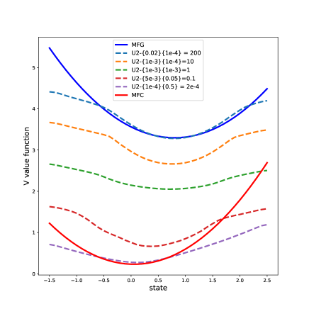
Figure 4: Numerical results of the two-timescale Q-learning algorithm where intermediate ratios $\rho^{Q}/\rho^{\mu}=10,1,0.1$ are adopted, in addition to numerically extreme ratios $\rho^{Q}/\rho^{\mu}=200,0.0002$.

7 Conclusion

In this work, by establishing the approximation diagram Fig. 1, we explain why the two-timescale Q-learning algorithm can converge to MFG or MFC solutions by tuning two learning rates. Based on our constructed Lyapunov function, we provide a novel unified convergence result for the algorithm for all ranges of learning rate ratios. It would be interesting to investigate what type of problems that the two-timescale Q-learning algorithm solves when $0<\rho^{Q}/\rho^{\mu}<\infty$, as shown in Figure 4. We guess that for the intermediate regime, devising a mixed model of MFG and MFC might be a reasonable approach, and we leave it as our future work. We believe that the idea of this Lyapunov function construction can shed lights on convergence proofs for other algorithms in the study of MFC and MFG.

Appendix A

The case of MFC problems need extra treatments due to the value function’s dependence on the changing population distribution. We thus consult the Itô-Lions’ formula in Wasserstein space studied in Buckdahn et al. (2017), and give a brief review of additional required assumptions in order to apply this Itô-Lions’ formula for MFC.

Consider the square-integrable space $\mathcal{P}(\mathcal{X})$, the lifting of functions $u:\mathcal{P}(\mathcal{X})\to{\mathbb{R}}$ is defined as $\tilde{u}(\xi):=u(P[\xi])$. We say that $u$ is differentiable (resp., $C^{1}$) on $\mathcal{P}(\mathcal{X})$ if the lift $\tilde{u}$ is Fréchet differentiable on $L^{2}(\mathcal{F};\mathcal{X})$, that is, there exists a linear continuous mapping $D\tilde{u}(\xi):L^{2}(\mathcal{F};\mathcal{X})\to{\mathbb{R}}$ such that

$$\tilde{u}(\xi+\eta)-\tilde{u}(\xi)=D\tilde{u}(\xi)(\eta)+\lito(\|\eta\|),$$ (A.1)

with $\|\eta\|\to 0$ for $\eta\in L^{2}(\mathcal{F};\mathcal{X})$. On the law $P[\xi]$, for $\xi,\xi^{\prime}\in L^{2}(\mathcal{F};\mathcal{X})$, one can write

$$u(P[\xi^{\prime}])-u(P[\xi])=\mathbb{E}[\partial_{\mu}u(P[\xi],\xi)\cdot(\xi^{\prime}-\xi)]+\lito(\|\xi^{\prime}-\xi\|)$$ (A.2)

to define $\partial_{\mu}u$. Moreover, the second derivative is defined as

$$\partial_{\mu}^{2}u(\mu,x,y):=\big{(}\partial_{\mu}\big{(}(\partial_{\mu}u)_{j}(\cdot,y)\big{)}(\mu,x)\big{)}_{1\leq j\leq d},\quad\text{for}~{}(\mu,x,y)\in\mathcal{P}(\mathcal{X})\times\mathcal{X}\times\mathcal{X}.$$ (A.3)

Let us state the expansion formula from Buckdahn et al. (2017):

Lemma 11 (Buckdahn et al. (2017), Lemma 2.1)

If $(\partial_{\mu}u)_{j}(\cdot,y)\in C_{b}^{1,1}(\mathcal{P}(\mathcal{X}))$ for all $y\in\mathcal{X},1\leq j\leq d$, $\partial_{\mu}u(\mu,\cdot)$ is differentiable for every $\mu\in\mathcal{P}(\mathcal{X})$, and $\partial_{\mu}^{2}u,\partial_{y}\partial_{\mu}u$ are bounded and Lipschitz continuous, then one has the second-order expansion

$$u(P[\xi^{\prime}])-u(P[\xi]) =\mathbb{E}[\partial_{\mu}u(P[\xi],\xi)\cdot\eta]+\frac{1}{2}\mathbb{E}\Big{[}\tilde{\mathbb{E}}\big{[}\operatorname{Tr}\big{(}\partial_{\mu}^{2}u(P[\xi],\tilde{\xi},\xi)\cdot\tilde{\eta}\otimes\eta\big{)}\big{]}\Big{]}$$ (A.4)

$$\quad+\frac{1}{2}\mathbb{E}\Big{[}\operatorname{Tr}\big{(}\partial_{y}\partial_{\mu}u(P[\xi],\xi)\cdot\eta\otimes\eta\big{)}\Big{]}+O(\|\eta\|^{3})$$

where $\eta=\xi^{\prime}-\xi$, and $\tilde{\mathbb{E}}[\cdot]=\int_{\tilde{\mathcal{X}}}(\cdot)d\tilde{P}$ associated with the copy $(\tilde{\mathcal{X}},\tilde{\mathcal{F}},\tilde{P})$ where $\tilde{P}[\tilde{\xi}]=P[\xi]$.

Now we are ready to restate the Theorem 3 with complete assumptions.

Theorem A.1

We assume that $\alpha$ is Lipschitz in $x$: there exists a constant $C_{\alpha}>0$ such that

$$\|\alpha(x_{1})-\alpha(x_{2})\|\leq C_{\alpha}\|x_{1}-x_{2}\|.$$ (A.5)

With Assumptions 1, 2, and 3, in addition to assumptions on $f$ in order to apply Lemma 11, we have the approximations that, for all $x\in{\mathcal{X}}$,

$$V_{h,\text{MFG}}^{\mu,\alpha}(x)=V_{\text{MFG}}^{\mu,\alpha}(x)+\bigo(h^{1/2}),$$ (A.6)

$$V_{h,\text{MFC}}^{\alpha}(x)=V_{\text{MFC}}^{\alpha}(x)+\bigo(h^{1/2}),$$

when $h\to 0$.

Proof  We may consider the discrete time iteration

$$X_{h}^{k+1}=b(X_{h}^{k},\alpha(X_{h}^{k}))h+\sigma(X_{h}^{k},\alpha(X_{h}^{k}))\sqrt{h}B_{k},$$ (A.7)

with $B_{k}\sim_{i.i.d}\mathcal{N}(0,I)$, which can be viewed as the Euler-Maruyama scheme of the SDE

$$dX_{t}=b(X_{t},\alpha_{t})dt+\sigma(X_{t},\alpha_{t})dB_{t}.$$ (A.8)

We ignore $b,\sigma$’s dependence on $\mu$ here by assuming the limiting distribution is fixed. It is well-known that the Euler-Maruyama scheme is an order $1/2$-scheme in the strong sense Kloeden et al. (2012). In other words, with Lipschitzness assumptions of $b,\sigma$, and a slight modification of the induction proof, one can conclude immediately that there exists a constant $C>0$ such that

$$\mathbb{E}\big{[}\|X_{h}^{k}-X_{kh}\|\big{|}X_{0}=x\big{]}\leq Ch^{1/2}$$ (A.9)

for all $k\geq 1$. Then, for $t\in[kh,(k+1)h)$, since

$$X_{t}=X_{kh}+\int_{kh}^{t}b(X_{s},\alpha_{s})ds+\int_{kh}^{t}\sigma(X_{s},\alpha_{s})dB_{s},$$ (A.10)

by Itô’s isometry and boundedness of $b,\sigma$, we get

$$\mathbb{E}\big{[}\|X_{t}-X_{kh}\|\big{|}X_{0}=x\big{]}\leq Ch^{1/2}.$$ (A.11)

Therefore, the triangle inequality gives that for $t\in[kh,(k+1)h)$,

$$\mathbb{E}\big{[}\|X_{h}^{k}-X_{t}\|\big{|}X_{0}=x\big{]}\leq Ch^{1/2}.$$ (A.12)

MFG:

We start from the definition of $V_{h,\text{MFG}}^{\mu,\alpha}$ and derive that

$$V_{h,\text{MFG}}^{\mu,\alpha}(x) =\mathbb{E}\left[h\sum_{k=0}^{\infty}e^{-\gamma kh}f(X_{h}^{k},\alpha(X_{h}^{k}),\mu)\bigg{|}X_{0}=x\right]$$ (A.13)

$$= \mathbb{E}\left[\sum_{k=0}^{\infty}\int_{kh}^{(k+1)h}e^{-\gamma kh}f(X_{h}^{k},\alpha(X_{h}^{k}),\mu)ds\bigg{|}X_{0}=x\right]$$

$$= \mathbb{E}\left[\int_{0}^{\infty}e^{-\gamma s}f(X_{s},\alpha(X_{s}),\mu)ds\bigg{|}X_{0}=x\right]$$

$$\quad+\mathbb{E}\left[\sum_{k=0}^{\infty}\int_{kh}^{(k+1)h}\Big{(}e^{-\gamma kh}f(X_{h}^{k},\alpha(X_{h}^{k}),\mu)-e^{-\gamma s}f(X_{s},\alpha(X_{s}),\mu)\Big{)}ds\bigg{|}X_{0}=x\right]$$

$$:=V_{\text{MFG}}^{\mu,\alpha}(x)+\mathcal{E}_{\text{MFG}},$$

and what remains is to estimate the error term $\mathcal{E}_{\text{MFG}}$. Apply the triangle inequality, we get

$$\big{|}\mathcal{E}_{\text{MFG}}\big{|} \leq\mathbb{E}\left[\sum_{k=0}^{\infty}\int_{kh}^{(k+1)h}\big{|}e^{-\gamma kh}-e^{-\gamma s}\big{|}\big{|}f(X_{h}^{k},\alpha(X_{h}^{k}),\mu)\big{|}ds\bigg{|}X_{0}=x\right]$$ (A.14)

$$\quad+\mathbb{E}\left[\sum_{k=0}^{\infty}\int_{kh}^{(k+1)h}e^{-\gamma s}\Big{|}f(X_{h}^{k},\alpha(X_{h}^{k}),\mu)-f(X_{s},\alpha(X_{s}),\mu)\Big{|}ds\bigg{|}X_{0}=x\right]$$

$$\leq\|f\|_{\infty}\sum_{k=0}^{\infty}\int_{kh}^{(k+1)h}\big{|}e^{-\gamma kh}-e^{-\gamma s}\big{|}ds+\tilde{L}\mathbb{E}\left[\sum_{k=0}^{\infty}\int_{kh}^{(k+1)h}e^{-\gamma s}\|X_{h}^{k}-X_{s}\|ds\bigg{|}X_{0}=x\right]$$

$$=\|f\|_{\infty}\bigo(h)\int_{0}^{\infty}e^{-\gamma s}ds+\tilde{L}\bigo(h^{1/2})\int_{0}^{\infty}e^{-\gamma s}ds=\bigo(h^{1/2})$$

for small $h$, where in the last inequality we use Assumption 1, Lipschitz assumption of $\alpha$, and take $\tilde{L}:=\max\{K_{x},K_{\alpha}C_{\alpha}\}$. Thus we conclude that

$$V_{h,\text{MFG}}^{\mu,\alpha}(x)=V_{\text{MFG}}^{\mu,\alpha}(x)+\lito(1),$$ (A.15)

as $h\to 0$.

MFC:

For the MFC case, we need to additionally deal with $f(x,a,\mu)$’s dependence on the changing distributions $\mu$. We again start from the definition of $V_{h,\text{MFC}}^{\alpha}$ and derive that

$$V_{h,\text{MFC}}^{\alpha}(x) =\mathbb{E}\left[h\sum_{k=0}^{\infty}e^{-\gamma kh}f(X_{h}^{k},\alpha(X_{h}^{k}),\mathcal{P}[X_{h}^{k}])\bigg{|}X_{0}=x\right]$$ (A.16)

$$= \mathbb{E}\left[\sum_{k=0}^{\infty}\int_{kh}^{(k+1)h}e^{-\gamma kh}f(X_{h}^{k},\alpha(X_{h}^{k}),\mathcal{P}[X_{h}^{k}])ds\bigg{|}X_{0}=x\right]$$

$$= \mathbb{E}\left[\int_{0}^{\infty}e^{-\gamma s}f(X_{s},\alpha(X_{s}),\mathcal{P}[X_{s}])ds\bigg{|}X_{0}=x\right]$$

$$\quad+\mathbb{E}\left[\sum_{k=0}^{\infty}\int_{kh}^{(k+1)h}\Big{(}e^{-\gamma kh}f(X_{h}^{k},\alpha(X_{h}^{k}),\mathcal{P}[X_{h}^{k}])-e^{-\gamma s}f(X_{s},\alpha(X_{s}),\mathcal{P}[X_{s}])\Big{)}ds\bigg{|}X_{0}=x\right]$$

$$:=V_{\text{MFC}}^{\alpha}(x)+\mathcal{E}_{\text{MFC}}.$$

The error term $\mathcal{E}_{\text{MFC}}$ can be further split into

$$\big{|}\mathcal{E}_{\text{MFC}}\big{|} \leq\mathbb{E}\left[\sum_{k=0}^{\infty}\int_{kh}^{(k+1)h}\big{|}e^{-\gamma kh}-e^{-\gamma s}\big{|}\big{|}f(X_{h}^{k},\alpha(X_{h}^{k}),\mathcal{P}[X_{h}^{k}])\big{|}ds\bigg{|}X_{0}=x\right]$$ (A.17)

$$\quad+\mathbb{E}\left[\sum_{k=0}^{\infty}\int_{kh}^{(k+1)h}e^{-\gamma s}\Big{|}f(X_{h}^{k},\alpha(X_{h}^{k}),\mathcal{P}[X_{h}^{k}])-f(X_{s},\alpha(X_{s}),\mathcal{P}[X_{h}^{k}])\Big{|}ds\bigg{|}X_{0}=x\right]$$

$$\quad+\mathbb{E}\left[\sum_{k=0}^{\infty}\int_{kh}^{(k+1)h}e^{-\gamma s}\Big{|}f(X_{s},\alpha(X_{s}),\mathcal{P}[X_{h}^{k}])-f(X_{s},\alpha(X_{s}),\mathcal{P}[X_{s}])\Big{|}ds\bigg{|}X_{0}=x\right]$$

$$:=I+II+III.$$

Apply the triangle inequality and Assumption 1 as we did for MFG, we get again that

$$I+II=O(h^{1/2}).$$ (A.18)

For $III$, we need to apply Lemma 11. By taking $\eta_{k,s}:=X_{h}^{k}-X_{s}$ and write $f(X_{s},\alpha(X_{s}),\cdot)\equiv f_{s}(\cdot)$, we have that

$$III =\mathbb{E}\left[\sum_{k=0}^{\infty}\int_{kh}^{(k+1)h}e^{-\gamma s}\mathbb{E}[\partial_{\mu}f_{s}(\mathcal{P}[X_{s}],X_{s})\cdot\eta_{k,s}]ds\bigg{|}X_{0}=x\right]$$ (A.19)

$$\quad+\mathbb{E}\left[\sum_{k=0}^{\infty}\int_{kh}^{(k+1)h}e^{-\gamma s}\frac{1}{2}\mathbb{E}\Big{[}\tilde{\mathbb{E}}\big{[}\operatorname{Tr}\big{(}\partial_{\mu}^{2}f_{s}(\mathcal{P}[X_{s}],\tilde{X_{s}},X_{s})\cdot\tilde{\eta}_{k,s}\otimes\eta_{k,s}\big{)}\big{]}\Big{]}ds\bigg{|}X_{0}=x\right]$$

$$\quad+\frac{1}{2}\mathbb{E}\left[\sum_{k=0}^{\infty}\int_{kh}^{(k+1)h}e^{-\gamma s}\mathbb{E}\Big{[}\operatorname{Tr}\big{(}\partial_{y}\partial_{\mu}V^{\alpha}_{h,MFC}(\mathcal{P}[x],x)\cdot\eta_{k,s}\otimes\eta_{k,s}\big{)}\Big{]}ds\bigg{|}X_{0}=x\right]$$

$$\quad+\mathbb{E}\left[\sum_{k=0}^{\infty}\int_{kh}^{(k+1)h}e^{-\gamma s}O(\|\eta_{k,s}\|^{3})ds\bigg{|}X_{0}=x\right]=O(h^{1/2}),$$

since the first term above dominates others as $\mathbb{E}[\|\eta_{k,s}\||X_{0}=x]\sim O(h^{1/2})$ for small $h$. Thus we conclude that

$$V_{h,\text{MFC}}^{\mu,\alpha}(x)=V_{\text{MFC}}^{\mu,\alpha}(x)+\lito(1),$$ (A.20)

as $h\to 0$.

References

• Angiuli et al. (2022) Andrea Angiuli, Jean-Pierre Fouque, and Mathieu Laurière. Unified reinforcement Q-learning for mean field game and control problems. Mathematics of Control, Signals, and Systems, 34(2):217–271, 2022.
• Angiuli et al. (2023) Andrea Angiuli, Jean-Pierre Fouque, Mathieu Laurière, and Mengrui Zhang. Convergence of multi-scale reinforcement q-learning algorithms for mean field game and control problems. arXiv preprint arXiv:2312.06659, 2023.
• Angiulia et al. (2023) Andrea Angiulia, Jean-Pierre Fouquea, and Mathieu Laurièreb. Reinforcement Learning for Mean Field Games, with Applications to Economics. Machine Learning and Data Sciences for Financial Markets: A Guide to Contemporary Practices, page 393, 2023.
• Bellman (1957) Richard Bellman. A markovian decision process. Journal of mathematics and mechanics, pages 679–684, 1957.
• Bensoussan et al. (2013) Alain Bensoussan, Phillip Yam, and Jens Frehse. Mean Field Games and Mean Field Type Control Theory. SpringerBriefs in Mathematics. Springer, 2013. ISBN 978-1-4614-8507-0. doi: 10.1007/978-1-4614-8508-7.
• Bertsekas (2019) Dimitri Bertsekas. Reinforcement learning and optimal control. Athena Scientific, 2019.
• Bhandari and Russo (2024) Jalaj Bhandari and Daniel Russo. Global optimality guarantees for policy gradient methods. Operations Research, 2024.
• Borkar (1997) Vivek S Borkar. Stochastic approximation with two time scales. Systems & Control Letters, 29(5):291–294, 1997.
• Borkar (2008) V.S. Borkar. Stochastic Approximation: A Dynamical Systems Viewpoint. Cambridge University Press, 2008. ISBN 9780521515924. URL https://books.google.com.hk/books?id=QLxIvgAACAAJ.
• Buckdahn et al. (2017) Rainer Buckdahn, Juan Li, Shige Peng, and Catherine Rainer. Mean-field stochastic differential equations and associated pdes. Annals of probability, 45(2):824–878, 2017.
• Busoniu et al. (2008) Lucian Busoniu, Robert Babuska, and Bart De Schutter. A comprehensive survey of multiagent reinforcement learning. IEEE Transactions on Systems, Man, and Cybernetics, Part C (Applications and Reviews), 38(2):156–172, 2008.
• Caines et al. (2006) Peter E Caines, Minyi Huang, and Roland P Malhamé. Large population stochastic dynamic games: closed-loop mckean-vlasov systems and the nash certainty equivalence principle. Communications in Information and Systems, 6(3):221–252, 2006.
• Carmona and Delarue (2018) René Carmona and François Delarue. Probabilistic theory of mean field games with applications I-II. Springer, 2018.
• Carmona et al. (2019) René Carmona, Mathieu Laurière, and Zongjun Tan. Linear-quadratic mean-field reinforcement learning: convergence of policy gradient methods. arXiv preprint arXiv:1910.04295, 2019.
• Carmona et al. (2023) René Carmona, Mathieu Laurière, and Zongjun Tan. Model-free mean-field reinforcement learning: mean-field mdp and mean-field q-learning. The Annals of Applied Probability, 33(6B):5334–5381, 2023.
• Cui and Koeppl (2021) Kai Cui and Heinz Koeppl. Approximately solving mean field games via entropy-regularized deep reinforcement learning. In International Conference on Artificial Intelligence and Statistics, pages 1909–1917. PMLR, 2021.
• Fu et al. (2019) Zuyue Fu, Zhuoran Yang, Yongxin Chen, and Zhaoran Wang. Actor-critic provably finds nash equilibria of linear-quadratic mean-field games. arXiv preprint arXiv:1910.07498, 2019.
• Gu et al. (2021) Haotian Gu, Xin Guo, Xiaoli Wei, and Renyuan Xu. Mean-field controls with q-learning for cooperative marl: convergence and complexity analysis. SIAM Journal on Mathematics of Data Science, 3(4):1168–1196, 2021.
• Gu et al. (2016) Shixiang Gu, Timothy Lillicrap, Ilya Sutskever, and Sergey Levine. Continuous deep q-learning with model-based acceleration. In International conference on machine learning, pages 2829–2838. PMLR, 2016.
• Guo et al. (2019) Xin Guo, Anran Hu, Renyuan Xu, and Junzi Zhang. Learning mean-field games. Advances in neural information processing systems, 32, 2019.
• Guo et al. (2022) Xin Guo, Renyuan Xu, and Thaleia Zariphopoulou. Entropy regularization for mean field games with learning. Mathematics of Operations research, 47(4):3239–3260, 2022.
• Hernandez-Leal et al. (2019) Pablo Hernandez-Leal, Bilal Kartal, and Matthew E Taylor. A survey and critique of multiagent deep reinforcement learning. Autonomous Agents and Multi-Agent Systems, 33(6):750–797, 2019.
• Hu and Laurière (2023) Ruimeng Hu and Mathieu Laurière. Recent developments in machine learning methods for stochastic control and games. arXiv preprint arXiv:2303.10257, 2023.
• Jia and Zhou (2023) Yanwei Jia and Xun Yu Zhou. q-learning in continuous time. Journal of Machine Learning Research, 24(161):1–61, 2023.
• Jiang and Jiang (2015) Yu Jiang and Zhong-Ping Jiang. Global adaptive dynamic programming for continuous-time nonlinear systems. IEEE Transactions on Automatic Control, 60(11):2917–2929, 2015.
• Kim and Yang (2020) Jeongho Kim and Insoon Yang. Hamilton-jacobi-bellman equations for q-learning in continuous time. In Learning for Dynamics and Control, pages 739–748. PMLR, 2020.
• Kim et al. (2021) Jeongho Kim, Jaeuk Shin, and Insoon Yang. Hamilton-Jacobi Deep Q-Learning for Deterministic Continuous-Time Systems with Lipschitz Continuous Controls. Journal of Machine Learning Research, 22(206):1–34, 2021. URL http://jmlr.org/papers/v22/20-1235.html.
• Kiran et al. (2021) B Ravi Kiran, Ibrahim Sobh, Victor Talpaert, Patrick Mannion, Ahmad A Al Sallab, Senthil Yogamani, and Patrick Pérez. Deep reinforcement learning for autonomous driving: A survey. IEEE Transactions on Intelligent Transportation Systems, 23(6):4909–4926, 2021.
• Kloeden et al. (2012) Peter Eris Kloeden, Eckhard Platen, and Henri Schurz. Numerical solution of SDE through computer experiments. Springer Science & Business Media, 2012.
• Kober et al. (2013) Jens Kober, J Andrew Bagnell, and Jan Peters. Reinforcement learning in robotics: A survey. The International Journal of Robotics Research, 32(11):1238–1274, 2013.
• Konda and Tsitsiklis (1999) Vijay Konda and John Tsitsiklis. Actor-critic algorithms. Advances in neural information processing systems, 12, 1999.
• Lasry and Lions (2007) Jean-Michel Lasry and Pierre-Louis Lions. Mean field games. Jpn. J. Math., 2(1):229–260, 2007. doi: https://doi.org/10.1007/s11537-007-0657-8.
• Laurière et al. (2022) Mathieu Laurière, Sarah Perrin, Matthieu Geist, and Olivier Pietquin. Learning mean field games: A survey. arXiv preprint arXiv:2205.12944, 2022.
• Meyn and Tweedie (2012) Sean P Meyn and Richard L Tweedie. Markov chains and stochastic stability. Springer Science & Business Media, 2012.
• Mguni et al. (2018) David Mguni, Joel Jennings, and Enrique Munoz de Cote. Decentralised learning in systems with many, many strategic agents. In Thirty-Second AAAI Conference on Artificial Intelligence, 2018.
• Mnih et al. (2013) Volodymyr Mnih, Koray Kavukcuoglu, David Silver, Alex Graves, Ioannis Antonoglou, Daan Wierstra, and Martin Riedmiller. Playing atari with deep reinforcement learning. arXiv preprint arXiv:1312.5602, 2013.
• Palanisamy et al. (2014) Muthukumar Palanisamy, Hamidreza Modares, Frank L Lewis, and Muhammad Aurangzeb. Continuous-time q-learning for infinite-horizon discounted cost linear quadratic regulator problems. IEEE transactions on cybernetics, 45(2):165–176, 2014.
• Silver et al. (2016) David Silver, Aja Huang, Chris J Maddison, Arthur Guez, Laurent Sifre, George Van Den Driessche, Julian Schrittwieser, Ioannis Antonoglou, Veda Panneershelvam, Marc Lanctot, et al. Mastering the game of go with deep neural networks and tree search. nature, 529(7587):484–489, 2016.
• Subramanian and Mahajan (2019) Jayakumar Subramanian and Aditya Mahajan. Reinforcement Learning in Stationary Mean-field Games. In Proceedings. 18th International Conference on Autonomous Agents and Multiagent Systems, 2019.
• Sutton and Barto (2018) Richard S Sutton and Andrew G Barto. Reinforcement learning: An introduction. MIT press, 2018.
• Tallec et al. (2019) Corentin Tallec, Léonard Blier, and Yann Ollivier. Making Deep Q-learning methods robust to time discretization. In Kamalika Chaudhuri and Ruslan Salakhutdinov, editors, Proceedings of the 36th International Conference on Machine Learning, volume 97 of Proceedings of Machine Learning Research, pages 6096–6104. PMLR, 09–15 Jun 2019.
• Vamvoudakis (2017) Kyriakos G Vamvoudakis. Q-learning for continuous-time linear systems: A model-free infinite horizon optimal control approach. Systems & Control Letters, 100:14–20, 2017.
• Wang et al. (2020) Haoran Wang, Thaleia Zariphopoulou, and Xun Yu Zhou. Reinforcement learning in continuous time and space: A stochastic control approach. The Journal of Machine Learning Research, 21(1):8145–8178, 2020.
• Wang et al. (2021) Weichen Wang, Jiequn Han, Zhuoran Yang, and Zhaoran Wang. Global convergence of policy gradient for linear-quadratic mean-field control/game in continuous time. In International Conference on Machine Learning, pages 10772–10782. PMLR, 2021.
• Watkins (1989) Christopher JCH Watkins. Learning from delayed rewards. PhD thesis, Cambridge University, Cambridge, England, 1989.
• Watkins and Dayan (1992) Christopher JCH Watkins and Peter Dayan. Q-learning. Machine learning, 8:279–292, 1992.
• Williams (1992) Ronald J Williams. Simple statistical gradient-following algorithms for connectionist reinforcement learning. Machine learning, 8:229–256, 1992.
• Yang et al. (2018) Yaodong Yang, Rui Luo, Minne Li, Ming Zhou, Weinan Zhang, and Jun Wang. Mean field multi-agent reinforcement learning. In International conference on machine learning, pages 5571–5580. PMLR, 2018.
• Yang et al. (2019) Zhuoran Yang, Yongxin Chen, Mingyi Hong, and Zhaoran Wang. Provably global convergence of actor-critic: A case for linear quadratic regulator with ergodic cost. Advances in neural information processing systems, 32, 2019.
• Zaman et al. (2023) Muhammad Aneeq Uz Zaman, Alec Koppel, Sujay Bhatt, and Tamer Basar. Oracle-free reinforcement learning in mean-field games along a single sample path. In International Conference on Artificial Intelligence and Statistics, pages 10178–10206. PMLR, 2023.
• Zeng et al. (2021) Sihan Zeng, Thinh T Doan, and Justin Romberg. A two-time-scale stochastic optimization framework with applications in control and reinforcement learning. arXiv preprint arXiv:2109.14756, 2021.
• Zhang et al. (2021) Kaiqing Zhang, Zhuoran Yang, and Tamer Başar. Multi-agent reinforcement learning: A selective overview of theories and algorithms. Handbook of reinforcement learning and control, pages 321–384, 2021.
• Zhou and Lu (2023) Mo Zhou and Jianfeng Lu. Single Timescale Actor-Critic Method to Solve the Linear Quadratic Regulator with Convergence Guarantees. Journal of Machine Learning Research, 24(222):1–34, 2023. URL http://jmlr.org/papers/v24/22-0644.html.