Gray-Box Nonlinear Feedback Optimization

Abstract

Feedback optimization enables autonomous optimality seeking of a dynamical system through its closed-loop interconnection with iterative optimization algorithms. Among various iteration structures, model-based approaches require the input-output sensitivity of the system to construct gradients, whereas model-free approaches bypass this need by estimating gradients from real-time evaluations of the objective. These approaches own complementary benefits in sample efficiency and accuracy against model mismatch, i.e., errors of sensitivities. To achieve the best of both worlds, we propose gray-box feedback optimization controllers, featuring systematic incorporation of approximate sensitivities into model-free updates via adaptive convex combination. We quantify conditions on the accuracy of the sensitivities that render the gray-box approach preferable. We elucidate how the closed-loop performance is determined by the number of iterations, the problem dimension, and the cumulative effect of inaccurate sensitivities. The proposed controller contributes to a balanced closed-loop behavior, which retains provable sample efficiency and optimality guarantees for nonconvex problems. We further develop a running gray-box controller to handle constrained time-varying problems with changing objectives and steady-state maps.

I Introduction

Efficient steady-state operation is crucial for engineering systems, e.g., power grids, process control systems, and communication networks [1, 2, 3]. To this end, numerical optimization offers solutions based on an explicit formulation of the problem, e.g., an economic efficiency objective together with constraints that encode the input-output map and forecasts or anticipated statistics of disturbances. While these solutions are ready to be implemented in an offline and feedforward fashion, their effectiveness may be jeopardized if the complex plant and unmeasured disturbances cannot be accurately modeled. Given the extensive use of feedback control for adaptation and robustness, it is desirable to pursue an optimal steady-state behavior through a closed-loop paradigm.

I-A Related Work

Closed-loop optimization has been explored from multiple perspectives. A core principle is to interact with the plant dynamics, learn from feedback, and improve the control strategies. Typical examples focusing on cumulative performance include model predictive control[4], real-time iterations[5], and reinforcement learning (RL)[6]. In these examples, iterative adjustments of strategies based on feedback are pivotal in handling inaccurate models or unknown dynamics and navigating through vast policy spaces.

In terms of closed-loop steady-state optimization, extremum seeking[7] is an effective solution that does not require any model information, i.e., it is model-free. The key idea is to add random exploration signals (e.g., sinusoids) and use averaging to obtain an update direction. Extremum seeking requires exploration signals of well-selected frequencies to avoid mutual interference, and therefore it is typically applied to low-dimensional problems. Constraint satisfaction is usually fulfilled in an asymptotic way through penalty or barrier functions[8]. The recent work [9] robustly handles constraints by introducing projection maps.

Feedback optimization[2, 1, 3] has emerged as a promising paradigm for steady-state optimization of dynamical systems. Compared to extremum seeking, it systematically handles high-dimensional objectives and constraints. The core insight is to implement optimization-based iterations as feedback controllers, thus driving a stable plant to an optimal steady state. Thanks to the use of real-time measurements, feedback optimization bypasses the need to explicitly access the complex input-output map and the unknown exogenous disturbance. Provided that the controller gain is low (i.e., a time-scale separation holds)[10, 11], closed-loop stability, optimality, and constraint satisfaction are guaranteed[12, 13, 14]. This closed-loop structure also facilitates tracking the trajectory of time-varying optimal solutions in non-stationary environments[15, 16, 17, 18] and proves effective in industry[19].

The manifold benefits of feedback optimization rely on the premise that the steady-state input-output sensitivity of the plant is available. This premise stems from using the chain rule to form the gradient-based adjustment direction of the controller. Although sensitivities may sometimes be available thanks to first-principle models and parameters[20, 19, 21], the general challenge of modeling complex, large-scale, and poorly known systems can render the use of sensitivities elusive, thereby causing closed-loop sub-optimality, constraint violation, or instability[2]. To address this issue, two streams of strategies have been explored in the literature.

One stream is model-based, in that the key model information (i.e., sensitivity) is learned from offline data or online interactions. Behavioral systems theory[22] enables data-driven representations of the sensitivity of a linear time-invariant plant via its historical trajectories[23, 24]. Moreover, recursive least-squares estimation allows learning sensitivities in an online fashion based on the streaming data of inputs and outputs[25, 26]. Nonetheless, if the sensitivity is not learned fast and accurately enough, the closed-loop behavior may still exhibit considerable sub-optimality, see [27, Section VI].

Another stream to address unknown sensitivities is model-free (or black-box), which avoids learning sensitivities altogether. The motivation is that such learning may become prohibitive for complex systems and involve errors (e.g., when input-output maps are non-differentiable) and large transients (e.g., for persistence of excitation). In the context of closed-loop optimization, model-free operations are achieved by employing iterative optimization schemes without gradient evaluations, thus circumventing the sensitivity owing to the chain rule. Some methods [28, 29] embrace the probabilistic framework of Bayesian optimization[30] and update the input as the maximizer of an acquisition function. While these methods enjoy good sample efficiency, they are mostly suitable for low-dimensional problems due to the bottleneck of modeling objectives via Gaussian processes. A different strategy is to leverage zeroth-order optimization[31] and construct stochastic gradient estimates from function evaluations. Examples include [32, 33, 34] that use multi-point estimates (i.e., multiple actuation steps per iteration) for algebraic maps, as well as [27] that only requires a single actuation step per iteration and handles dynamical systems in real time. Overall, the stochasticity of gradient estimates may affect the convergence rate, thus causing an increase in the required number of actuations compared to model-based approaches.

I-B Motivations

Models encode useful structural information. This feature contributes to the high sample efficiency (i.e., fast convergence) of model-based controllers. However, it also poses strong requirements for the accuracy of models that should be either formulated or learned online. Model-free operations are attractive because they offer provable guarantees without resorting to complex models. Nevertheless, they can be less sample-efficient due to stochastic exploration or restricted to certain classes of problems (e.g., in low-dimensional spaces).

Given such complementary benefits, it is promising to develop gray-box approaches to achieve the best of both worlds. The power of gray-box strategies has been showcased in various problems, e.g., RL[35, 36], predictive control[37], and stabilization[38]. Some methods are built upon model-based pipelines and introduce model-free, learning-based blocks for inference or improvement, including estimating initial states [39], generating feedforward inputs[21], and learning terminal costs and constraints[37]. Others augment model-free pipelines with model-based priors (e.g., prior mean [40] or a model-based policy as a warm start[41]) or utilize synthetic data generated from transition models to enhance training in model-free RL[35, 42]. Furthermore, recent works on learning-augmented control[38, 43] combine a model-based (albeit sub-optimal) policy with a black-box, machined-learned policy. This viewpoint of combination is related to [44] that fuses policies given by multiple candidate models. However, the tuning of the combination coefficients therein requires accessing system matrices or identification errors of states, which may not always be available in applications.

While the above contributions are inspiring, it is unclear how gray-box approaches can be designed and proven useful in the context of steady-state optimization. In applications, although the accurate input-output sensitivity of a system can be elusive, we may know an approximation through prior knowledge, first-principle models, or estimation[20, 19, 21]. These approximate sensitivities can play an important role in the gray-box pipeline. Apart from the differences in the problem setup, some questions related to performance metrics are also unexplored. How to quantify the conditions favoring gray-box approaches over model-based or model-free methods, and vice versa? How to establish provable improvement using the same performance measure for all approaches? In this article, we will address these questions by developing and examining gray-box feedback optimization controllers that utilize approximate sensitivities to optimize the closed-loop steady-state behavior.

I-C Contributions

We develop gray-box feedback optimization controllers combining the complementary benefits of model-based and model-free approaches. The main contributions are summarized as follows.

• We propose a gray-box feedback optimization controller to drive a stable nonlinear system to an optimal steady-state operating point quantified by a nonconvex objective. When implemented in closed loop, this controller uses real-time outputs and iteratively adjusts inputs by adaptively combining model-based inexact gradients from approximate sensitivities and model-free gradient estimates.

• We characterize the conditions on the accuracy of sensitivities that render the gray-box controller preferable to its model-based counterparts. These conditions and the flexibility of our adaptive combination equip the proposed controller with versatility, such that it applies when there is only coarse prior knowledge and when any suitable sensitivity learning scheme is employed.

• We evaluate the closed-loop behavior via the squared gradient norm of the nonconvex objective and characterize its dependence on cumulative errors of sensitivities. The gray-box controller overcomes the issue of sub-optimality, which troubles model-based controllers using sensitivities with slowly vanishing errors. It can also exploit sensitivities of lower quality (e.g., with bounded errors) to improve sample efficiency compared to model-free approaches.

• We extend the gray-box controller to address time-varying problems involving changing objectives, variable disturbances, and fixed input constraint sets. We quantify the closed-loop behavior through dynamic regret and the error of tracking solution trajectories, which focus on the cumulative gap against the optimal benchmark and the last-iterate guarantee, respectively. For both performance measures, the gray-box controller is shown to strike an excellent balance between sample efficiency and accuracy despite approximate sensitivities.

I-D Organization

The rest of this article is organized as follows. In Section II, we provide the problem of interest and some preliminaries. Section III presents the design of the gray-box controller. The performance guarantees in a static and unconstrained setting are established in Section IV. Section V extends the design and analysis to handle time-varying problems with input constraints. We perform numerical evaluations in Section VI. Finally, Section VII concludes this article.

II Problem Formulation and Preliminaries

II-A Problem Formulation

Consider a fast stable system abstracted by its nonlinear steady-state input-output map $h:\mathbb{R}^{p}\times\mathbb{R}^{r}\to\mathbb{R}^{q}$

$$y=h(u,d),$$ (1)

where $u\in\mathbb{R}^{p}$ is the input, $y\in\mathbb{R}^{q}$ is the output, and $d\in\mathbb{R}^{r}$ is the unknown exogenous disturbance.

We aim to find an input $u$ to optimize the steady-state operation of the system (1), i.e.,

$$\begin{split}\min_{u\in\mathbb{R}^{p},y\in\mathbb{R}^{q}}\quad&\Phi(u,y)\\ \text{s.t.}\quad&y=h(u,d).\end{split}$$ (2)

In problem (2), the objective $\Phi:\mathbb{R}^{p}\times\mathbb{R}^{q}\to\mathbb{R}$ is a (nonconvex) function of the input $u$ and the steady-state output $y$ of the system (1). Let $\tilde{\Phi}(u)\triangleq\Phi(u,h(u,d))$ be the reduced objective function. Some assumptions are as follows.

Assumption 1.

The steady-state map $h(u,d)$ is differentiable with respect to $u$.

Assumption 2.

The function $\tilde{\Phi}(u)$ is $M$-Lipschitz continuous and $L$-smooth (i.e., its gradients are $L$-Lipschitz continuous). It satisfies $\tilde{\Phi}^{*}\triangleq\inf_{u\in\mathbb{R}^{p}}\tilde{\Phi}(u)>-\infty$.

Assumption 3.

The function $\Phi(u,y)$ is $M_{\Phi}$-Lipschitz with respect to $y$.

Assumption 1 is typically satisfied for general systems. For instance, a stable linear dynamical system admits a linear differentiable steady-state map[11]. For a nonlinear dynamical system, the (local) existence and differentiability of its steady-state map can be ensured by the implicit function theorem (see [45, Theorem 1B.1]) with suitable requirements on its dynamics equations. The above properties of the objective function are relatively weak, commonly assumed (e.g., [46, 47]), and satisfied in many applications[1].

Remark 1.

In this article, we consider nonlinear systems abstracted by steady-state maps to streamline exposition. We can establish similar guarantees when confronted with nonlinear dynamics by introducing converse Lyapunov functions and analyzing the coupled evolution of system dynamics and controller iterations, see also [10, 16, 27]. We will present the corresponding numerical evaluations in Section VI.

A tempting solution to problem (2) is to directly use numerical optimization solvers. Nonetheless, solvers require the explicit expression of the steady-state map $h$ and the exact value of the disturbance $d$. These requirements can be hard to satisfy when complex systems and unknown disturbances are involved. Hence, we pursue a feedback optimization controller that utilizes real-time output measurements to iteratively drive the system (1) to an optimal operating point minimizing (2).

Model-based feedback optimization controllers[12, 10, 25, 26] learn and use the input-output sensitivity $\nabla_{u}h(u,d)$ of the plant (1) and iteratively update inputs by following the gradient of $\tilde{\Phi}(u)=\Phi(u,h(u,d))$. After invoking the chain rule, their update rule reads as

$$u_{k+1}=u_{k}\!-\!\eta(\nabla_{u}\Phi(u_{k},y_{k})\!+\!\nabla_{u}h(u_{k},d)^{\top}\nabla_{y}\Phi(u_{k},y_{k})),$$ (3)

where $\eta>0$ is a step size, and $y_{k}$ is the output of the plant (1) at time $k\in\mathbb{N}$. Model-free controllers[33, 34, 27] bypass the information on sensitivities and rely purely on stochastic exploration. Their trade-offs in sample efficiency and solution accuracy are discussed in Section I-B. In contrast, we will merge approximate sensitivities (obtained, among others, through prior knowledge or recursive estimation) into model-free updates, thus achieving the best of both worlds.

Remark 2.

We consider a differentiable map (1) and a smooth objective $\tilde{\Phi}$ as common grounds to theoretically compare different controllers. The gray-box controllers in this article also allow non-smooth steady-state maps and objectives thanks to their structures of combination. This feature implies a broad scope of applications.

II-B Preliminaries of Gradient Estimation

Various model-free feedback optimization controllers (e.g., [33, 34, 27]) exploit zeroth-order optimization[31]. Their underlying key idea is to iteratively update in the direction of negative gradient estimates. Such estimates are constructed from function evaluations and random exploration vectors.

Consider a smooth function $\xi:\mathbb{R}^{p}\to\mathbb{R}$. Let $\delta>0$ be a smoothing parameter and $v\in\mathbb{R}^{p}$ be a vector uniformly sampled from the unit sphere $\mathbb{S}_{p-1}\triangleq\{v\in\mathbb{R}^{p}:\|v\|=1\}$, i.e., $v\sim U(\mathbb{S}_{p-1})$. The smooth approximation $\xi_{\delta}$ of $\xi$ is

$$\xi_{\delta}(w)=\operatorname{\mathbb{E}}_{v^{\prime}\sim U(\mathbb{B}_{p})}[\xi(w+\delta v^{\prime})],$$ (4)

where $w\in\mathbb{R}^{p}$, and $\mathbb{B}_{p}\triangleq\{v^{\prime}\in\mathbb{R}^{p}:\|v^{\prime}\|\leq 1\}$ is the closed unit ball in $\mathbb{R}^{p}$. The following lemma summarizes the construction of a gradient estimate and useful properties of $\xi_{\delta}$.

Lemma 1 ([48, Lemma 4.1]).

If $\xi:\mathbb{R}^{p}\to\mathbb{R}$ is $L_{\xi}$-smooth, then $\xi_{\delta}(w)$ defined in (4) is also $L_{\xi}$-smooth, and

$$\operatorname{\mathbb{E}}_{v\in U(\mathbb{S}_{p-1})}\left[\frac{p}{\delta}\xi(w+\delta v)v\right] =\nabla\xi_{\delta}(w),$$ (5a)

$$|\xi_{\delta}(w)-\xi(w)| \leq\frac{L_{\xi}\delta^{2}}{2},$$ (5b)

$$\|\nabla\xi_{\delta}(w)-\nabla\xi(w)\| \leq\frac{L_{\xi}p\delta}{2},$$ (5c)

where $w\in\mathbb{R}^{p}$, $\delta>0$. If $\xi$ is convex, then $\xi_{\delta}$ is also convex.

Lemma 1 implies that $\frac{p}{\delta}\xi(w\!+\!\delta v)v$ constructed from the function value $\xi(w\!+\!\delta v)$ and the random vector $v$ is an unbiased (zeroth-order) estimate of $\nabla\xi_{\delta}(w)$. Further, the closeness between the values and gradients of $\xi$ and $\xi_{\delta}$ can be adjusted to arbitrary precision via the smoothing parameter $\delta$. To connect back to feedback optimization, a gradient estimate as in (5a) can be employed to update the actuation $u$ in lieu of the model-based gradient as in (3), see [27] for further reading.

III Design of the Gray-Box Controller

III-A Gray-Box Controller

For a given input $u_{k}$ at time $k\in\mathbb{N}$, suppose that we have access to an approximate input-output sensitivity matrix $\hat{H}_{k}\in\mathbb{R}^{q\times p}$, which differs from the true sensitivity $H_{k}\triangleq\nabla_{u}h(u_{k},d)$. Such an approximate sensitivity can be obtained through prior knowledge, first-principle models[20, 19, 21], or online learning and estimation[25, 49].

Our proposed feedback controller iteratively adjusts control inputs by using real-time output measurements. The update direction is constructed by adaptively fusing an inexact gradient from the approximate sensitivity $\hat{H}_{k}$ and a gradient estimate based on stochastic exploration. The update rules are

$$w_{k+1} =w_{k}-\eta\tilde{\phi}_{k},$$ (6a)

$$\tilde{\phi}_{k} =\alpha_{k}\tilde{\phi}_{k,1}+(1-\alpha_{k})\tilde{\phi}_{k,2},$$ (6b)

$$\tilde{\phi}_{k,1} =\nabla_{u}\Phi(u_{k},y_{k})+\hat{H}_{k}^{\top}\nabla_{y}\Phi(u_{k},y_{k}),$$ (6c)

$$\tilde{\phi}_{k,2} =\frac{pv_{k}}{\delta}\big{(}\Phi(u_{k},y_{k})-\Phi(u_{k-1},y_{k-1})\big{)},$$ (6d)

$$u_{k+1} =w_{k+1}+\delta v_{k+1},$$ (6e)

where $w_{k}$ is a candidate solution, $\alpha_{k}\in[0,1]$ is a convex combination coefficient whose design is further specified in Section III-B, $\eta>0$ is a step size, $\delta>0$ is a smoothing parameter, $p$ is the size of the input, and $v_{0},\ldots,v_{k}\sim U(\mathbb{S}_{p-1})$ are independent and identically distributed (i.i.d.) random variables sampled from the unit sphere $\mathbb{S}_{p-1}$.

In the iterative update (6), the gray-box controller merges two descent directions via the adaptive convex combination (6b). The first one (i.e., $\tilde{\phi}_{k,1}$ in (6c)) is an inexact gradient using $\hat{H}_{k}$. The second one (i.e., $\tilde{\phi}_{k,2}$ in (6d)) is a gradient estimate constructed from the current and previous evaluations of the objective $\Phi$, which has been originally developed in [46] and leveraged for feedback optimization in our previous work [27]. Note that $\tilde{\phi}_{k,2}$ is useful since it is an unbiased estimate of $\nabla\tilde{\Phi}_{\delta}(w_{k})$, where $\tilde{\Phi}_{\delta}$ is the smooth approximation of $\tilde{\Phi}$. The controller perturbs the new candidate solution $w_{k+1}$ by an exploration noise $\delta v_{k}$, see (6e). This perturbation helps to explore $\tilde{\Phi}$ around $w_{k+1}$, thereby facilitating the construction of the gradient estimate. Finally, the obtained input $u_{k+1}$ is applied to the plant. Fig. 1 illustrates the closed-loop interconnection of the physical plant (1) and our gray-box feedback optimization controller (6).

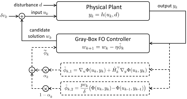
Figure 1: Interconnection of a physical plant (1) and the gray-box feedback optimization controller (6).

III-B Adaptive Combination Coefficients

A key ingredient of our gray-box feedback optimization controller (6) is the combination coefficient $\alpha_{k}$. This coefficient helps to blend the approximate sensitivity $\hat{H}_{k}$ with model-free updates. We discuss how to tune it in different scenarios based on the quality of $\hat{H}_{k}$.

If we can learn the sensitivity $H_{k}$ sufficiently fast and accurately, e.g., via Kalman filtering[25], then model-based controllers augmented with online sensitivity estimation [25, 26] are certainly favorable. Specifically, we will show in Theorem 5 and Corollary 6 later on that the condition favoring model-based controllers is whenever

$$\epsilon_{H,k}\triangleq\|\hat{H}_{k}-H_{k}\|\leq\frac{\mkern 1.5mu\overline{\mkern-1.5mu\epsilon\mkern-1.5mu}\mkern 1.5mu^{\prime}}{(k+1)^{\theta}},\quad\theta\geq\frac{1}{3},\quad k\in\mathbb{N},$$ (7)

where $\epsilon_{H,k}$ is the error of $\hat{H}_{k}$ compared to $H_{k}$, and $\mkern 1.5mu\overline{\mkern-1.5mu\epsilon\mkern-1.5mu}\mkern 1.5mu^{\prime}>0$ is a pre-specified initial error bound. Condition (7) can be satisfied, e.g., when we use recursive least squares to learn sensitivities evolving by linear random processes[25]. However, different issues (e.g., noisy measurements, lack of covariance information, nonlinear dynamics, or resource constraints) can render sensitivity estimation slow or inaccurate, if not impossible. When this happens, model-based controllers cease to be favorable, and our gray-box approach (6) is advantageous. We then distinguish two general cases related to $\hat{H}_{k}$ and present the corresponding strategies for tuning $\alpha_{k}$ in (6b).

Case 1: Approximate Sensitivity with a Bounded Error

In many applications, we construct approximate sensitivities based on prior knowledge or first-principle models[20, 19, 21], which are then fixed during online operation. This practice corresponds to the case where a bounded error exists between the approximate sensitivity $\hat{H}_{k}$ and the ground-truth $H_{k}$, i.e.,

$$\epsilon_{H,k}=\|\hat{H}_{k}-H_{k}\|\leq\mkern 1.5mu\overline{\mkern-1.5mu\epsilon\mkern-1.5mu}\mkern 1.5mu,\quad k\in\mathbb{N},$$ (8)

where $\mkern 1.5mu\overline{\mkern-1.5mu\epsilon\mkern-1.5mu}\mkern 1.5mu>0$. In this case, we select a constant $C>0$ and use the following vanishing combination coefficient

$$\alpha_{k}=\min\Big{\{}\frac{C}{(k\!+\!1)^{\frac{2}{3}}},1\Big{\}},\quad k\in\mathbb{N}.$$ (9)

Case 2: Asymptotically Accurate Sensitivity

Online estimation techniques can be incorporated to generate increasingly accurate estimates of sensitivities based on the trajectory of the plant (1). However, we may not always learn sensitivities sufficiently fast due to measurement errors, lack of covariance data, etc. For instance, the estimation error of the sensitivity may decrease as

$$\epsilon_{H,k}=\|\hat{H}_{k}\!-\!H_{k}\|\leq\frac{\mkern 1.5mu\overline{\mkern-1.5mu\epsilon\mkern-1.5mu}\mkern 1.5mu^{\prime}}{(k+1)^{\theta}},~{}\theta\in\Big{(}0,\frac{1}{3}\Big{)},~{}k\in\mathbb{N},$$ (10)

where $\mkern 1.5mu\overline{\mkern-1.5mu\epsilon\mkern-1.5mu}\mkern 1.5mu^{\prime}>0$ is an error bound. It implies that the estimate $\hat{H}_{k}$ asymptotically converges to $H_{k}$, but the convergence rate is not quite fast. In this case, we choose a constant $C^{\prime}>0$ and leverage the following vanishing combination coefficient

$$\alpha_{k}=\min\Big{\{}\frac{C^{\prime}}{(k\!+\!1)^{\frac{2}{3}-2\theta}},1\Big{\}},\quad k\in\mathbb{N}.$$ (11)

Since $\alpha_{k}$ starts from $1$ and approaches $0$ as $k$ increases, the rules (9) and (11) initially favor the model-based inexact gradient $\tilde{\phi}_{k,1}$ for rapid response and later the model-free gradient estimate $\tilde{\phi}_{k,2}$ for solution accuracy.

Our gray-box controller applies when no sensitivity learning is performed and when any appropriate learning technique is employed to estimate sensitivities, as long as the characterization of learning rates as (10) is available. Such versatility arises from the structure of adaptive combination (6b) and the conditions (8) and (10).

The reason why different adaptive combination coefficients are needed in these different cases can be understood by examining the error of the inexact gradient $\tilde{\phi}_{k,1}$ (see (6c)) compared to the true gradient $\nabla\tilde{\Phi}(u_{k})$ due to $\hat{H}_{k}$, i.e.,

$$\epsilon_{k}\!\triangleq\!\nabla\tilde{\Phi}(u_{k})\!-\!\tilde{\phi}_{k,1}\!=\!(H_{k}\!-\!\hat{H}_{k})^{\top}\nabla_{y}\Phi(u_{k},y_{k}),~{}k\!\in\!\mathbb{N}.$$ (12)

In fact, the combination coefficients in (9) and (11) help to adjust the scaled cumulative error $\sum_{k=0}^{T-1}\alpha_{k}\operatorname{\mathbb{E}}_{v_{[T]}}[\|\epsilon_{k}\|^{2}]$ incurred by our gray-box controller (6). Here $T\in\mathbb{N}_{+}$ is the number of iterations, and $\operatorname{\mathbb{E}}_{v_{[T]}}[\cdot]$ denotes the expectation with respect to the collection of i.i.d. samples $v_{[T]}\triangleq\{v_{0},\ldots,v_{T-1}\}$. The following lemma quantifies the order of this scaled cumulative error, which will then be useful in the analysis of the performance.

Lemma 2.

Let Assumption 3 hold. If the approximate sensitivity $\hat{H}_{k}$ satisfies (8) (or (10)), then the gray-box controller (6) with the combination coefficients given in (9) (respectively, in (11)) ensures that the error in (12) satisfies

$$\sum_{k=0}^{T-1}\alpha_{k}\operatorname{\mathbb{E}}_{v_{[T]}}[\|\epsilon_{k}\|^{2}]=\mathop{}\mathopen{}\mathcal{O}\mathopen{}\left(T^{\frac{1}{3}}\right).$$ (13)

Proof.

Please see Appendix -B. ∎

IV Performance Analysis and Comparison

We now establish a performance certificate when our proposed gray-box controller (6) is interconnected in closed loop with the system (1). Then, we compare this certificate with those of model-based and model-free feedback optimization controllers, thereby highlighting that our gray-box approach achieves the best of both worlds.

IV-A Performance Certificate

First, we provide a recursive inequality of the second moment $\operatorname{\mathbb{E}}_{v_{[k]}}[\|\tilde{\phi}_{k}\|^{2}]$, where $\tilde{\phi}_{k}$ is the update direction (6a) of our gray-box controller (6). This inequality reflects the progress of the controller and helps to establish our closed-loop performance certificate.

Lemma 3.

If Assumptions 1 and 2 hold, the update rule (6) implies that

$$\operatorname{\mathbb{E}}_{v_{[k]}}[\|\tilde{\phi}_{k}\|^{2}]$$

$$\leq\frac{4(1\!-\!\alpha_{k})^{2}}{\delta^{2}}p^{2}M^{2}\eta^{2}\operatorname{\mathbb{E}}_{v_{[k]}}[\|\tilde{\phi}_{k-1}\|^{2}]\!+\!8\alpha_{k}^{2}\operatorname{\mathbb{E}}_{v_{[k]}}[\|\nabla\tilde{\Phi}(w_{k})\|^{2}]$$

$$\quad+48(1\!-\!\alpha_{k})^{2}p^{2}\operatorname{\mathbb{E}}_{v_{[k]}}[\|\nabla\tilde{\Phi}(w_{k-1})\|^{2}]+4\alpha_{k}^{2}\operatorname{\mathbb{E}}_{v_{[k]}}[\|\epsilon_{k}\|^{2}]$$

$$\quad+8\alpha_{k}^{2}L^{2}\delta^{2}+6(1\!-\!\alpha_{k})^{2}L^{2}p^{2}\delta^{2}.$$ (14)

Proof.

Please see Appendix -C. ∎

We now characterize the performance of the closed-loop interconnection of the plant (1) and the controller (6), where $\eta$, $\delta$, and $\alpha_{k}$ are the step size, the smoothing parameter, and the combination coefficient, respectively. Moreover, $p$ is the size of the input, $T$ is the number of iterations set beforehand, and $\epsilon_{H,k}$ is the error of the approximate sensitivity $\hat{H}_{k}$.

Theorem 4.

Suppose that Assumptions 1-3 hold. Let $0<\eta\leq 1/224Lp^{2}T^{\frac{1}{3}}$ and $\delta=\sqrt{2}M/112LT^{\frac{1}{3}}$. The closed-loop interconnection of the plant (1) and the gray-box controller (6) results in

$$\frac{1}{T}\sum_{k=0}^{T-1}\operatorname{\mathbb{E}}_{v_{[T]}}[\|\nabla\tilde{\Phi}(w_{k})\|^{2}]$$

$$\leq 896L(\operatorname{\mathbb{E}}_{v_{[T]}}[\tilde{\Phi}(w_{0})]-\tilde{\Phi}^{*})\frac{p^{2}}{T^{\frac{2}{3}}}+\frac{5M_{\Phi}^{2}}{T}\sum_{k=0}^{T-1}\alpha_{k}\epsilon_{H,k}^{2}$$

$$\quad+\frac{M^{2}}{112^{2}T^{\frac{5}{3}}}\sum_{k=0}^{T-1}\left(8\alpha_{k}+p^{2}(1-\alpha_{k})\right)+\frac{C_{M,\|\tilde{\phi}_{0}\|^{2}}}{T},$$ (15)

where $C_{M,\|\tilde{\phi}_{0}\|^{2}}>0$ is a constant that depends on $M$ and $\|\tilde{\phi}_{0}\|^{2}$ but not $p$ and $T$. Furthermore, with $\hat{H}_{k}$ satisfying (8) (or (10)) and the designs of $\{\alpha_{k}\}_{k=0}^{T-1}$ as in (9) (respectively, in (11)), the closed-loop interconnection satisfies

$$\frac{1}{T}\sum_{k=0}^{T-1}\operatorname{\mathbb{E}}_{v_{[T]}}[\|\nabla\tilde{\Phi}(w_{k})\|^{2}]=\mathop{}\mathopen{}\mathcal{O}\mathopen{}\left(\frac{p^{2}}{T^{\frac{2}{3}}}\right).$$ (16)

Proof.

Please see Appendix -E. ∎

In Theorem 4, $\eta$ and $\delta$ are constants that rely on the specified number of iterations $T$, and they are fixed during online implementations. The performance measure is the average of the squared gradient norms of the reduced objective $\tilde{\Phi}$ at the candidate solutions $\{w_{k}\}_{k=0}^{T-1}$. This measure reflects the local optimality (i.e., stationarity) of these solutions in terms of the nonconvex objective $\tilde{\Phi}$[34, 27], and it is typical in the literature on nonconvex optimization, see [31, 50].

The upper bound (4) elucidates how the model-based direction (6c) and the model-free estimate (6d) shape the overall performance. Specifically, the term $5M_{\Phi}^{2}/T\sum_{k=0}^{T\!-\!1}\alpha_{k}\epsilon_{H,k}^{2}$ quantifies the cumulative error when the approximate sensitivity $\hat{H}_{k}$ is used instead of the true sensitivity $H_{k}$, whereas $M^{2}/(112^{2}T^{\frac{5}{3}})\sum_{k=0}^{T\!-\!1}p^{2}(1\!-\!\alpha_{k})$ results from the accumulation of the inherent bias of the gradient estimate, see (5c). The combination coefficients $\{\alpha_{k}\}_{k=0}^{T-1}$ prescribed in Lemma 2 help to achieve a balanced performance of our gray-box controller (6) and result in the rate (16). Initially, we choose $\alpha_{k}$ close to $1$, thus exploiting the model-based direction (6c) to quickly approach the neighborhood of solutions. This design also facilitates regulating the term $\sum_{k=0}^{T-1}(8\alpha_{k}+p^{2}(1-\alpha_{k}))$ in (4) for high-dimensional problems (i.e., with large $p$). Afterward, we tune $\alpha_{k}$ close to $0$ to suppress the cumulative error arising from approximate sensitivities. That is, we leverage the model-free estimate (6d) more to seek solution accuracy. Overall, as the number of iterations $T$ increases, the convergence measure in (16) approaches zero, which suggests local optimality in terms of the nonconvex problem (2).

IV-B Comparison with Model-based and Model-Free Controllers

To demonstrate the merits of our gray-box approach (6), we compare it with the (deterministic) model-based and model-free feedback optimization controllers.

First, we characterize the sub-optimality of the deterministic and model-based feedback optimization controller (3) that uses approximate sensitivities. It is a special case of (6), though it uses only the inexact gradient $\tilde{\phi}_{k,1}$ (i.e., the combination coefficients are $\alpha_{k}=1,\forall k\in\mathbb{N}$) and does not require exploration signals (i.e., the smoothing parameter $\delta=0$).

Theorem 5.

Suppose that Assumptions 1-3 hold. Consider the deterministic and model-based controller whose update rule is given by (6) with $\alpha_{k}=1,\forall k\in\mathbb{N}$ and $\delta=0$. Let $0<\eta\leq 1/4L$. The closed-loop interconnection of the plant (1) and this controller results in

$$\frac{1}{T}\sum_{k=0}^{T-1}\|\nabla\tilde{\Phi}(w_{k})\|^{2}\leq\frac{16L\big{(}\tilde{\Phi}(w_{0})\!-\!\tilde{\Phi}^{*}\big{)}}{T}+\frac{3M_{\Phi}^{2}}{T}\sum_{k=0}^{T-1}\epsilon_{H,k}^{2}.$$ (17)

Moreover, if $\{\hat{H}_{k}\}_{k=0}^{T-1}$ satisfies (7), then

$$\frac{1}{T}\sum_{k=0}^{T-1}\|\nabla\tilde{\Phi}(w_{k})\|^{2}=\mathop{}\mathopen{}\mathcal{O}\mathopen{}\left(\frac{1}{T^{\frac{2}{3}}}\right).$$ (18)

Proof.

Please see Appendix -F. ∎

Note that (17) is not a special case of (4) for $\alpha_{k}=1$, and Theorem 5 requires a separate proof to obtain sharper results. Compared to (6), model-based controllers allow using a larger step size $\eta$, and the performance certificate (17) does not depend on the dimension $p$ of the problem. If the sensitivity is learned sufficiently fast and accurately (i.e., (7) holds), then model-based controllers achieve a better order of complexity (18) than that (see (16)) of our gray-box controller (6).

However, if the accuracy requirement (7) on sensitivities is not met, then the sub-optimality resulting from the cumulative errors in gradients due to $\hat{H}_{k}$ becomes more prominent. As quantified by the last term of (17), this sub-optimality cannot be adjusted by tuning algorithm parameters. If the error in $\hat{H}_{k}$ is non-vanishing as $k$ increases, then even for a large number of iterations $T$, the convergence measure may suffer from a non-zero residue. For instance, if $\hat{H}_{k}$ satisfies (8), then a constant upper bound on this residue is $3\mkern 1.5mu\overline{\mkern-1.5mu\epsilon\mkern-1.5mu}\mkern 1.5muM_{\Phi}^{2}$. In contrast, our gray-box controller (6) allows regulating sub-optimality by tuning the combination coefficients $\{\alpha_{k}\}_{k=0}^{T-1}$, thereby handling inaccurate sensitivities and relaxing the accuracy requirement of sensitivity learning. The following corollary summarizes the conditions on the accuracy of sensitivities that favor either the model-based or the gray-box controllers.

Corollary 6.

If approximate sensitivities $\{\hat{H}_{k}\}_{k=0}^{T-1}$ satisfy (7), then the upper bound (18) for the model-based controller in Theorem 5 is preferable to the one (i.e., (4)) in Theorem 4. If $\{\hat{H}_{k}\}_{k=0}^{T-1}$ satisfy (8) or (10), then the upper bound (16) for the gray-box controller in Theorem 4 is smaller.

Now we quantify the performance of the model-free feedback optimization controller [27]. This controller is also a special case of (6) with the combination coefficients $\alpha_{k}=0,\forall k\in\mathbb{N}$, because it constantly uses the gradient estimate (6d). By setting $\alpha_{k}=0$ in (4) we obtain the following:

Theorem 7.

Let the conditions of Theorem 4 hold. The closed-loop interconnection of the plant (1) and the model-free controller (i.e., (6) with $\alpha_{k}=0,\forall k\in\mathbb{N}$) results in

$$\frac{1}{T}\sum_{k=0}^{T-1}\operatorname{\mathbb{E}}_{v_{[T]}}[\|\nabla\tilde{\Phi}(w_{k})\|^{2}]$$

$$\leq\left(896L(\operatorname{\mathbb{E}}_{v_{[T]}}[\tilde{\Phi}(w_{0})]\!-\!\tilde{\Phi}^{*})\!+\!\frac{M^{2}}{112^{2}}\right)\frac{p^{2}}{T^{\frac{2}{3}}}\!+\!\frac{C^{\prime}_{M,\|\tilde{\phi}_{0}\|^{2}}}{T},$$ (19)

where $C^{\prime}_{M,\|\tilde{\phi}_{0}\|^{2}}>0$ is a constant that depends on $M$ and $\|\tilde{\phi}_{0}\|^{2}$ but not $p$ and $T$.

The upper bound (7) is different from the characterization in [27], because here we consider a smooth objective and a plant abstracted by its steady-state map. This bound implies that if the number of iterations $T$ set beforehand is large enough, then the model-free controller ensures that the convergence measure approaches zero. Compared to the bound (4) related to the gray-box controller in Theorem 4, in (7) there is no cumulative error of $\epsilon_{H,k}^{2}$ stemming from approximate sensitivities. For high-dimensional problems (i.e., when $p$ is large), the bound (7) can be larger than the bound (4), which may indicate lower sample efficiency of the controller in worst-case scenarios. We will further illustrate the difference in terms of the transient behavior between the model-free controller and the gray-box controller in Section VI.

V Constrained and Time-Varying Feedback Optimization

In Sections II and III, we examined a static and unconstrained problem of optimizing the steady-state performance of the plant (1), where the objective function and the exogenous disturbance are fixed. In some applications, however, both of them may change with time due to the variations of performance measures or parametric values. For instance, the objective may shift owing to tracking time-varying set points for voltages or power flows, and the changing disturbance results from volatile renewable generation[1, 2]. Moreover, the control inputs are usually constrained due to physical actuation limits, coupling economic requirements, etc. Consequently, instead of finding a fixed optimal solution, the goal becomes competing against or tracking time-varying optimal solutions while satisfying constraints. Thus, new controller designs and performance characterizations are needed. In this section, we present a running gray-box controller to handle constrained and time-varying problems.

V-A Problem Formulation

The above specifications of changing objectives, variable disturbances, and input constraints lead to constrained and time-varying optimization problems of the form

$$\begin{split}\min_{u\in\mathbb{R}^{p},y\in\mathbb{R}^{q}}~{}&\Phi_{k}(u,y)\\ \text{s.t.}~{}&y=h(u,d_{k}),\\ ~{}&u\in\mathcal{U}.\end{split}$$ (20)

In problem (20), $\Phi_{k}:\mathbb{R}^{p}\times\mathbb{R}^{q}\to\mathbb{R}$ and $d_{k}\in\mathbb{R}^{r}$ are the objective and the unknown disturbance at time $k\in\mathbb{N}$, respectively. Moreover, $\mathcal{U}\subset\mathbb{R}^{p}$ is the constraint set for $u$. Problem (20) involves optimizing the input-output performance of the following time-varying steady-state map

$$y=h(u,d_{k}).$$ (21)

In closed-loop implementations, we iteratively adjust the input $u$ after the output $y$ encoding $d_{k}$ is measured and the current objective $\Phi_{k}$ is revealed. Let $\tilde{\Phi}_{k}(u)\triangleq\Phi_{k}(u,h(u,d_{k}))$ be the reduced objective at time $k$. Our assumptions are as follows.

Assumption 4.

The set $\mathcal{U}$ is a closed, convex set with diameter $D>0$, i.e., $\forall u_{1},u_{2}\in\mathcal{U},\|u_{1}-u_{2}\|\leq D$.

Assumption 5.

The function $\tilde{\Phi}_{k}(u)$ is convex, $L_{k}$-smooth, and $M_{k}$-Lipschitz with respect to $u$. The function $\Phi_{k}(u,y)$ is $M_{\Phi,k}$-Lipschitz with respect to $y$. Moreover, $\{L_{k}\}$, $\{M_{k}\}$, and $\{M_{\Phi,k}\}$ are bounded.

Let $\mathcal{U}_{\tau}\triangleq\{u+\tau v|u\in\mathcal{U},v\in\mathbb{B}_{p}\}$ denote a set inflated from $\mathcal{U}$ by a limited range $\tau\mathbb{B}_{p}$, where $\tau>0$ is an expansion coefficient, and $\mathbb{B}_{p}$ is the closed unit ball in $\mathbb{R}^{p}$. The following assumption specifies the boundedness of $\tilde{\Phi}_{k}$.

Assumption 6.

The function $\tilde{\Phi}_{k}(u)$ is uniformly bounded, i.e., $\exists G\geq 0,\exists\tau>0,\forall u\in\mathcal{U}_{\tau},\forall k\in\mathbb{N},|\tilde{\Phi}_{k}(u)|\leq G$.

Assumptions 4-6 are typical in the literature, e.g., [51, 52, 53, 54]. Assumption 4 also implies that the norm of any point in $\mathcal{U}$ is bounded, i.e., $\exists\mkern 1.5mu\overline{\mkern-1.5muD\mkern-1.5mu}\mkern 1.5mu\geq 0,\forall u\in\mathcal{U},\|u\|\leq\mkern 1.5mu\overline{\mkern-1.5muD\mkern-1.5mu}\mkern 1.5mu$. Assumption 6 is related to Assumptions 4 and 5, because a continuous function defined on a compact set is bounded.

The unknown map $h$ and the changing disturbances $\{d_{k}\}$ may prevent us from directly solving (20) via numerical solvers. In contrast, we aim to develop a closed-loop, online strategy, featuring a feedback optimization controller that exploits output measurements to optimize the dynamic behavior of (1). Let $u_{k}^{*}\in\mathbb{R}^{p}$ be an optimal point of problem (20) at time $k$. The goal is to generate control inputs that are competitive with or track the sequence of optimal solutions $\{u_{k}^{*}\}_{k\in\mathbb{N}}$.

V-B Design of the Running Gray-Box Controller

To handle the constrained and time-varying problem (20), we adjust our gray-box controller (6) by leveraging projection and the most recent output measurement. The update rules are

$$w_{k+1} =\operatorname{Proj_{\mathcal{U}}}(w_{k}-\eta\hat{\phi}_{k}),$$ (22a)

$$\hat{\phi}_{k} =\alpha_{k}\hat{\phi}_{k,1}+(1-\alpha_{k})\hat{\phi}_{k,2},$$ (22b)

$$\hat{\phi}_{k,1} =\nabla_{u}\Phi_{k}(u_{k},y_{k})+\hat{H}_{k}^{\top}\nabla_{y}\Phi_{k}(u_{k},y_{k}),$$ (22c)

$$\hat{\phi}_{k,2} =\frac{pv_{k}}{\delta}\big{(}\Phi_{k}(u_{k},y_{k})-\Phi_{k-1}(u_{k-1},y_{k-1})\big{)},$$ (22d)

$$u_{k+1} =w_{k+1}+\delta v_{k+1},$$ (22e)

where $w_{k}$ is a candidate solution, $\operatorname{Proj_{\mathcal{U}}}(\cdot)$ denotes the projection to the constraint set $\mathcal{U}$, $\eta>0$ is a step size, $\alpha_{k}\in[0,1]$ is a convex combination coefficient, $\delta\in(0,\tau)$ is a smoothing parameter, $p$ is the size of the input, and $v_{0},\ldots,v_{k+1}\sim U(\mathbb{S}_{p-1})$ are i.i.d. random variables sampled from the unit sphere $\mathbb{S}_{p-1}$. Moreover, $\hat{H}_{k}\in\mathbb{R}^{q\times p}$ is an approximate sensitivity that differs from the true sensitivity $H_{k}\triangleq\nabla_{u}h(u_{k},d_{k})$. Note that $\hat{H}_{k}$ can be obtained via prior knowledge or online estimation, see also Section III-A.

Analogous to (6), in the iterative update our running gray-box controller (22) merges two directions. The first one (i.e., $\tilde{\phi}_{k,1}$ in (22c)) is an inexact gradient constructed from $\hat{H}_{k}$, whereas the second (i.e., $\tilde{\phi}_{k,2}$ in (22d)) is a stochastic gradient estimate. The controller subsequently performs a projection (see (22a)) to the constraint set $\mathcal{U}$, thus ensuring that the candidate solution $w_{k+1}$ satisfies the constraint. Finally, the solution is perturbed by $\delta v_{k+1}$ to form the input $u_{k+1}$ (see (22e)), and this input is applied to (21). Our controller (22) uses the latest information at time $k$ (i.e., the partial gradients and values of the current objective $\tilde{\Phi}_{k}$) to adapt to the variation of problem (20), which is different from (6).

Remark 3.

While the candidate solution $w_{k}$ lies in $\mathcal{U}$, the input $u_{k}$ in the transient stage may violate the constraint. If we need strict constraint satisfaction, we can project in (22a) onto a deflated set $(1-\kappa)\mathcal{U}$ as [52, 53], where $\kappa>0$.

Similar to Section III-B, for problem (20), model-based controllers purely using $\{\hat{H}_{k}\}_{k\in\mathbb{N}}$ (i.e., (22) with $\alpha_{k}=1,\forall k\in\mathbb{N}$) are favorable provided that $\hat{H}_{k}$ is a sufficiently accurate estimate of $H_{k}$, or more specifically,

$$\epsilon_{H,k}\triangleq\|\hat{H}_{k}-H_{k}\|\leq\frac{\mkern 1.5mu\overline{\mkern-1.5mu\epsilon\mkern-1.5mu}\mkern 1.5mu^{\prime}}{(k+1)^{\theta}},\quad\theta\geq\frac{1}{4},\quad k\in\mathbb{N},$$ (23)

where $\mkern 1.5mu\overline{\mkern-1.5mu\epsilon\mkern-1.5mu}\mkern 1.5mu^{\prime}>0$. The lower bound on $\theta$ in (23) is different from the one in (7) because of the changes in the problem setting and the convergence measure. Nonetheless, (23) may not always hold due to various issues, e.g., noisy measurements or nonlinear dynamics. In such a case, our proposed gray-box approach (22) is favorable. We analyze two cases of $\hat{H}_{k}$ and show how to select the combination coefficient $\alpha_{k}$ in (22b).

Case 1: Approximate Sensitivity with a Bounded Error

Consider $\hat{H}_{k}$ with an error $\epsilon_{H,k}$ that satisfies (8). Similar to (9), we use the following vanishing combination coefficient

$$\alpha_{k}=\min\Big{\{}\frac{C}{(k\!+\!1)^{\frac{1}{4}}},1\Big{\}},\quad k\in\mathbb{N}.$$ (24)

Case 2: Asymptotically Accurate Sensitivity

Various issues discussed in Section III-B may lead to $\hat{H}_{k}$ with an estimation error decreasing as

$$\epsilon_{H,k}=\|\hat{H}_{k}-H_{k}\|\leq\frac{\mkern 1.5mu\overline{\mkern-1.5mu\epsilon\mkern-1.5mu}\mkern 1.5mu^{\prime}}{(k+1)^{\theta}},~{}~{}\theta\in\Big{(}0,\frac{1}{4}\Big{)},~{}~{}k\in\mathbb{N},$$ (25)

where $\mkern 1.5mu\overline{\mkern-1.5mu\epsilon\mkern-1.5mu}\mkern 1.5mu^{\prime}>0$. When (25) arises, analogous to (11), we utilize the following vanishing coefficient

$$\alpha_{k}=\min\Big{\{}\frac{C^{\prime}}{(k\!+\!1)^{\frac{1}{4}-\theta}},1\Big{\}},\quad k\in\mathbb{N}.$$ (26)

The above choices of $\alpha_{k}$ regulate the scaled cumulative error due to $\hat{H}_{k}$. The intuition is similar to that of Lemma 2.

V-C Performance Certificates

We analyze the closed-loop interconnection of the plant (21) with our running gray-box controller (22). This controller updates the input in real time after measuring the output and evaluating the partial gradients and values of the current objective. We provide two non-asymptotic performance certificates. The first one is dynamic regret that reflects the transient behavior[54, 51, 52, 53, 55]. We focus on the cumulative difference in objective values when the sequence of decisions is compared to that of optimal solutions. The second certificate is the finite-time tracking error that offers a last-iterate guarantee[1, 56, 57]. We characterize this tracking error through the initial condition, the number of iterations, and the maximum per-step variation of optimal points. This certificate is in the flavor of input-to-state stability and akin to [12, 16, 14, 17].

To establish these performance certificates, we introduce a lemma that gives an upper bound on the expected distance between the descent direction $\hat{\phi}_{k}$ in (22b) used by our gray-box controller and the true gradient $\nabla\tilde{\Phi}_{k}(w_{k})$. Recall that $\epsilon_{H,k}=\|\hat{H}_{k}-H_{k}^{\prime}\|$ is the error of the approximate sensitivity $\hat{H}_{k}$ compared to the true sensitivity $H_{k}^{\prime}$.

Lemma 8.

Let Assumptions 1,4-6 hold. The update rule (22) ensures that

$$\operatorname{\mathbb{E}}_{v_{[k]}}[\|\hat{\phi}_{k}-\nabla\tilde{\Phi}_{k}(w_{k})\|]$$

$$\leq\alpha_{k}M_{\Phi,k}\epsilon_{H,k}\!+\!(1\!-\!\alpha_{k})\frac{2pG}{\delta}\!+\!L_{k}\delta\Big{(}\alpha_{k}\!+\!(1\!-\!\alpha_{k})\frac{p}{2}\Big{)}\triangleq\gamma_{k}.$$ (27)

Proof.

Please see Appendix -G. ∎

The upper bound (8) demonstrates the joint influences of the model-based direction (22c) and the model-free estimate (22d), which correspond to the terms containing $\alpha_{k}$ and $1-\alpha_{k}$, respectively. These joint influences can be adjusted through the combination coefficient $\alpha_{k}$.

We proceed to offer our first performance certificate, namely dynamic regret. It is the cumulative difference between the objective values evaluated at the candidate solutions $\{w_{k}\}_{k=1}^{T}$ and those at the optimal points $\{u_{k}^{*}\}_{k=1}^{T}$. To capture the variation of (20), we introduce the path length $C_{T}\triangleq\sum_{k=1}^{T}\|u_{k}^{*}\!-\!u_{k-1}^{*}\|$, which accumulates the shifts between two consecutive optimal points [54]. The following theorem characterizes the dynamic regret incurred by the closed-loop system.

Theorem 9.

Suppose that Assumptions 1,4-6 hold. Consider approximate sensitivities $\{\hat{H}_{k}\}_{k=1}^{T}$ that satisfy (23), (8), or (25). Let $\eta=1/p^{\frac{2}{3}}T^{\frac{3}{4}}$ and $\delta=\min(p^{\frac{1}{3}}/T^{\frac{1}{4}},\tau)$. The closed-loop interconnection of the plant (21) and the gray-box controller (22) incurs the following dynamic regret

$$\operatorname{Reg_{\mathnormal{T}}^{\mathnormal{d}}} \triangleq\sum_{k=1}^{T}\!\big{(}\operatorname{\mathbb{E}}_{v_{[T]}}[\tilde{\Phi}_{k}(w_{k})]\!-\!\tilde{\Phi}_{k}(u_{k}^{*})\big{)}$$

$$=\mathop{}\mathopen{}\mathcal{O}\mathopen{}\left(p^{\frac{2}{3}}T^{\frac{3}{4}}(C_{T}+1)\!+\!\sum_{k=1}^{T}\!\alpha_{k}\epsilon_{H,k}\right).$$ (28)

Furthermore, given $\hat{H}_{k}$ that satisfies (8) (or (25)) and $\{\alpha_{k}\}_{k\in\mathbb{N}}$ are designed as in (24) (respectively, in (26)), this closed-loop interconnection ensures that

$$\operatorname{Reg_{\mathnormal{T}}^{\mathnormal{d}}}=\mathop{}\mathopen{}\mathcal{O}\mathopen{}\left(p^{\frac{2}{3}}T^{\frac{3}{4}}(C_{T}+1)\right).$$ (29)

Proof.

Please see Appendix -H. ∎

The order of the dynamic regret (9) is determined by two major parts. The first part is proportional to the path length $C_{T}$, and the second part reflects the error accumulation due to $\hat{H}_{k}$. Recall that model-based controllers correspond to (22) with $\alpha_{k}=1,\forall k\in\mathbb{N}$ and $\delta=0$. For those controllers, when $\hat{H}_{k}$ satisfies (8) or (25), the second part (i.e., $\sum_{k=1}^{T}\alpha_{k}\epsilon_{H,k}$) will be of the orders of $\mathop{}\mathopen{}\mathcal{O}\mathopen{}\left(T\right)$ or $\mathop{}\mathopen{}\mathcal{O}\mathopen{}\left(T^{1-\theta}\right)$, respectively, where $0<\theta<\frac{1}{4}$. With the same choice of $\eta$ as in Theorem 9, the corresponding orders of $\operatorname{Reg_{\mathnormal{T}}^{\mathnormal{d}}}$ become $\mathcal{O}(p^{\frac{2}{3}}T^{\frac{3}{4}}(C_{T}+1)+T)$ and $\mathcal{O}(p^{\frac{2}{3}}T^{\frac{3}{4}}(C_{T}+1)+T^{1-\theta})$. In contrast, our gray-box controller (22) allows tuning $\{\alpha_{k}\}_{k=1}^{T}$ to arrive at (29). We will further illustrate the difference in the magnitude of $\operatorname{Reg_{\mathnormal{T}}^{\mathnormal{d}}}$ between the gray-box controller and the model-free controller (i.e., (22) with $\alpha_{k}=0,\forall k\in\mathbb{N}$) in Section VI.

Remark 4.

If the path length $C_{T}$ is known in advance (e.g., via quantitative sensitivity bounds[58]), then the order of $\operatorname{Reg_{\mathnormal{T}}^{\mathnormal{d}}}$ in (9) can be refined to $\mathcal{O}\big{(}p^{\frac{2}{3}}T^{\frac{3}{4}}\sqrt{C_{T}+1}\!+\!\sum_{k=1}^{T}\!\alpha_{k}\epsilon_{H,k}\big{)}$ by choosing the step size $\eta=\sqrt{C_{T}+1}/p^{\frac{2}{3}}T^{\frac{3}{4}}$. For model-based controllers using accurate $H_{k}$, we recover an expected regret bound of the order of $\mathcal{O}(\sqrt{T}(C_{T}+1))$ by selecting $\eta=1/\sqrt{T}$.

Now we present our second performance certificate, i.e., the finite-time tracking error $\operatorname{\mathbb{E}}_{v_{[T]}}[\|w_{T}-u_{T}^{*}\|]$ at time $T\in\mathbb{N}$. To facilitate characterization, we need a strong convexity assumption as follows.

Assumption 7.

The function $\tilde{\Phi}_{k}(u)$ is $\mu_{k}$-strongly convex, $L_{k}$-smooth, and $M_{k}$-Lipschitz with respect to $u$. The function $\Phi_{k}(u,y)$ is $M_{\Phi,k}$-Lipschitz with respect to $y$. Moreover, $\{L_{k}\}$, $\{M_{k}\}$, and $\{M_{\Phi,k}\}$ are bounded.

The strong convexity requirement in Assumption 7 is also found in [56, 57]. It ensures that there is a unique optimal solution $u_{k}^{*}$ to problem (20) at every time $k$. Hence, the tracking error $\operatorname{\mathbb{E}}_{v_{[T]}}[\|w_{T}-u_{T}^{*}\|]$ is well-defined. Let $\sigma_{u^{*}}\triangleq\sup_{k=1,\ldots,T}\|u_{k}^{*}-u_{k-1}^{*}\|$ be the supremum of the per-step variation of the optimal solutions $\{u_{k}^{*}\}_{k=0}^{T}$ to problem (20). The following theorem characterizes this tracking error.

Theorem 10.

Suppose that Assumptions 1, 4, 6, 7 hold. Let $\eta\in(0,2/\max_{k\in\mathbb{N}}L_{k})$ and $\delta\in(0,\tau)$. For the closed-loop interconnection of the plant (21) and the gray-box controller (22), we have

$$\operatorname{\mathbb{E}}_{v_{[T]}} [\|w_{T}-u_{T}^{*}\|]$$

$$\leq\rho^{T}\|w_{0}-u_{0}^{*}\|+\eta\sum_{k=0}^{T-1}\rho^{T-1-k}\gamma_{k}+\frac{\sigma_{u^{*}}}{1-\rho},$$ (30)

where $\rho\triangleq\max_{k=0,\ldots,T-1}\left\{\max\{|1-\eta\mu_{k}|,|1-\eta L_{k}|\}\right\}\in(0,1)$, and $\gamma_{k}$ is given by (8).

Proof.

Please see Appendix -I. ∎

Theorem 10 quantifies the finite-time tracking error as a function of the initial condition, the number of iterations, and the supremum of the per-step variation of optimal solutions. The influence of the initial condition is vanishing exponentially. The solution $w_{T}$ will asymptotically converge to a neighborhood of the optimal solution $u_{T}^{*}$, and the radius of this neighborhood is proportional to $\sigma_{u^{*}}$ and the weighted accumulation of $\{\gamma_{k}\}$. As discussed above in Lemma 8, the formula of $\gamma_{k}$ suggests the interplay of the error of the approximate sensitivity and the bias of the gradient estimate, which correspond to the model-based direction (22c) and the model-free estimate (22d), respectively.

VI Numerical Evaluations

We numerically evaluate the performance of our proposed gray-box controllers. As discussed in Remark 1, we extend theoretical results and explore the steady-state optimization of a nonlinear dynamical system. This system is

$$x_{k+1} =Ax_{k}+B_{1}u_{k}+B_{2}\sin(u_{k})+Ed_{x},$$ (31)

$$y_{k} =Cx_{k}+Dd_{y},$$

where $x\in\mathbb{R}^{20}$, $u\in\mathbb{R}^{10}$, and $y\in\mathbb{R}^{5}$ denote the state, input, and output, respectively, and $d_{x},d_{y}\in\mathbb{R}^{5}$ are disturbances. We draw the elements of the system matrices in (31) from the normal distribution. We further scale $A$ to let its spectral radius be $0.05$, i.e., the dynamics are quickly contracting. The disturbances $d_{x},d_{y}$ are sampled from the multivariate normal distribution, and their exact values are unknown beforehand.

First, we focus on the unconstrained and nonconvex problem

$$\min_{u\in\mathbb{R}^{10},y\in\mathbb{R}^{5}}~{}\Phi(u,y)=-\lambda\|u\|^{3}+u^{\top}M_{1}u+m_{2}^{\top}u+\|y\|^{2}$$

$$\hskip 20.00003pt\text{s.t.}~{}y=C(I\!-\!A)^{-1}(B_{1}u\!+\!B_{2}\sin(u)\!+\!Ed_{x})+Dd_{y}$$

$$\hskip 20.00003pt\phantom{\text{s.t.}~{}y}\triangleq h^{\prime}(u,d_{x},d_{y}),$$ (32)

where $M_{1}=M_{3}^{\top}M_{3}\in\mathbb{R}^{10\times 10}$ is positive definite, $m_{2}\in\mathbb{R}^{10}$, $\lambda=5\times 10^{-3}$, and the elements of $m_{2}$ and $M_{3}$ are drawn from the normal distribution. Due to $-\lambda\|u\|^{3}$ and the nonlinear part $\sin(u)$, the reduced objective $\tilde{\Phi}(u)\triangleq\Phi(u,h^{\prime}(u,d_{x},d_{y}))$ is nonconvex. Moreover, the equality constraint in (VI) corresponds to the steady-state map of the system (31). The input-output sensitivity matrix $H_{k}$ of (31) at $u_{k}$ is

$$H_{k}=C(I-A)^{-1}(B_{1}+B_{2}\operatorname{diag}(\cos(u_{k}))),$$

where $\operatorname{diag}(\cos(u_{k}))$ is a diagonal matrix with its diagonal entries given by $\cos(u_{k})$.

We compare the closed-loop interconnection of the system (31) with various controllers: model-based feedback optimization controllers with accurate $H_{k}$ and inexact $\hat{H}$, the controller with sensitivity learning [25], the model-free controller in [27], and our proposed gray-box controller (6) using $\hat{H}$. Specifically, $\hat{H}$ is generated by perturbing $C(I-A)^{-1}B_{1}$ with uniform noises, where the noise bound is $10\%$ of the maximum magnitude of the elements of $C(I-A)^{-1}B_{1}$. That is, $\hat{H}$ is a noisy estimate of the sensitivity corresponding to the linear part of (31). The step sizes are $\eta=2.5\times 10^{-4}$ for model-based controllers with $H_{k}$ or $\hat{H}$, the controller with sensitivity learning, as well as our gray-box controller (6). The model-free controller with such a step size will diverge. Thus, we select $\eta=2\times 10^{-4}$ for this controller. For the model-free and gray-box controllers, we choose the smoothing parameter $\delta=10^{-3}$ and conduct $30$ independent experiments. The gray-box controller uses (9) to determine the combination coefficients, and the constant $C$ therein is set to $100$.

Fig. 2 illustrates the performance of the closed-loop interconnection of the system (31) with the above controllers. The convergence measure is the squared gradient norm of the reduced objective $\tilde{\Phi}$ of (VI). The shades corresponding to the model-free and gray-box controllers represent the ranges of change in $30$ experiments, and the solid curves denote the averages. When the true sensitivity $H_{k}$ is available, the model-based controller enjoys both fast convergence and high accuracy. However, the use of an inexact sensitivity $\hat{H}$ causes a severe bias and closed-loop sub-optimality. Sensitivity learning addresses this issue via another unit of recursive estimation. This unit brings fluctuations and additional costs of storage and computation. The model-free controller yields rather accurate solutions, though there is an increase in the number of iterations required. In contrast, the gray-box controller strikes a balance between the convergence rate and the solution accuracy. Furthermore, the gray-box controller is easy to implement, in that it merely incorporates $\hat{H}$ but not more accurate sensitivity estimates via adaptive convex combination.

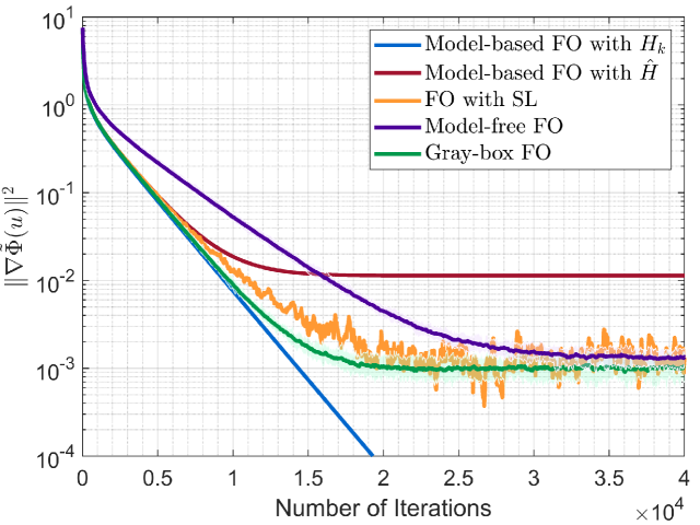
Figure 2: Comparison of our gray-box feedback optimization controller (6) and its counterparts to solve problem (VI). In the legend “FO” and “SL” stand for “feedback optimization” and “sensitivity learning”, respectively.

Next, we consider time-varying problems with input constraints. We aim to optimize the steady-state input-output performance of the system (31) as characterized by

$$\begin{split}\min_{u\in\mathbb{R}^{10},y\in\mathbb{R}^{5}}&~{}\Phi(u,y)=u^{\top}M_{1}u+m_{2}^{\top}u+\|y\|^{2}\\ \text{s.t.}&~{}y=h^{\prime}(u,d_{x},d_{y}),\\ &~{}\underline{u}\leq u\leq\mkern 1.5mu\overline{\mkern-1.5muu\mkern-1.5mu}\mkern 1.5mu,\end{split}$$ (33)

where $h^{\prime}(u,d_{x},d_{y})$ is the steady-state map of the system (31), and $\underline{u}\in\mathbb{R}^{10}$ and $\mkern 1.5mu\overline{\mkern-1.5muu\mkern-1.5mu}\mkern 1.5mu\in\mathbb{R}^{10}$ denote the lower bound and the upper bound on $u$, respectively. We generate $\underline{u}$ and $\mkern 1.5mu\overline{\mkern-1.5muu\mkern-1.5mu}\mkern 1.5mu$ from the multivariate normal distribution. Problem (33) is time-varying in that every $5\times 10^{3}$ iteration, $m_{2}$ and the positive definite $M_{1}$ in the objective are regenerated from normal distributions, and the disturbances $d_{x},d_{y}$ are regenerated from uniform distributions. Though the objective in (33) is nonconvex in $u$ because of the nonlinear term $\sin(u)$ in the map $h^{\prime}$, we obtain the comparator sequence $\{u_{k}^{*}\}$ by calling the fmincon function of MATLAB.

We augment the above controllers with projection onto the constraint set (similar to (22a)) and implement them in closed loop with the system (31). Specifically, the approximate sensitivity $\hat{H}$ is a perturbed version of $C(I-A)^{-1}B$, and the element-wise relative error is not more than $30\%$. The model-based controller, the controller with sensitivity learning[25], and our proposed gray-box controller (22) all utilize $\hat{H}$. We set the corresponding step sizes as $\eta=7.5\times 10^{-5}$. The model-free controller[27] experiences divergence with this step size, and, therefore, we select $\eta=5\times 10^{-5}$ in this case. The smoothing parameter is $\delta=10^{-3}$. We set $C=1$ in the rule (24) adopted by the gray-box controller to tune $\alpha_{k}$.

Fig. 3 illustrates the evolutions of the time-averaged dynamic regret (i.e., $\operatorname{Reg_{\mathnormal{T}}^{\mathnormal{d}}}/T$) incurred by such closed-loop interconnections. We observe similar patterns as Fig. 2. The direct use of the approximate sensitivity $\hat{H}$ diminishes solution accuracy. Nonetheless, by suitably incorporating this information, the gray-box controller achieves a better performance compared to the model-free controller and the controller with sensitivity learning. Further, for the considered iteration range it closely matches the benchmark with the exact sensitivity.

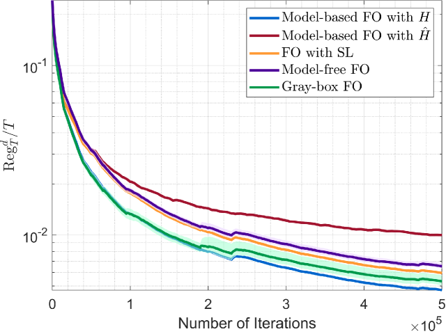
Figure 3: Comparison of different controllers when interconnected with the system (31) to solve the time-varying problem (33).

VII Conclusion

In this article, we proposed gray-box feedback optimization controllers to optimize the steady-state performance of a nonlinear system in closed loop. These controllers merge approximate input-output sensitivities of the system into model-free updates via adaptive convex combination. We quantified the accuracy conditions of the sensitivities that render the gray-box approaches preferable, and we provided design guidelines for setting combination coefficients therein. We demonstrated that the gray-box controllers exploit approximate sensitivities for sample efficiency, and that they circumvent error accumulation and ensure solution accuracy. For both the unconstrained static problem and the constrained time-varying problem, the proposed controllers combine the complementary benefits of model-based and model-free approaches.

Future directions include leveraging other forms of prior knowledge or model information, tackling output constraints via dualization, as well as analyzing the interplay between model-free control and online identification.

-A Auxiliary Lemmas

Let $a,b\in\mathbb{R}^{p}$ be any $p$-dimensional vectors. The following lemma gives the upper bounds on $a^{\top}b$ and $\|a+b\|^{2}$.

Lemma 11.

For any $a,b\in\mathbb{R}^{p}$, we have

$$a^{\top}b \leq\frac{1}{2}\left(\|a\|^{2}+\|b\|^{2}\right),$$ (34a)

$$\|a+b\|^{2} \leq 2\|a\|^{2}+2\|b\|^{2}.$$ (34b)

Proof.

The proof follows from the Cauchy-Schwarz inequality and the inequality $\forall a_{1},a_{2}\in\mathbb{R},2a_{1}a_{2}\leq a_{1}^{2}+a_{2}^{2}$. ∎

We provide an upper bound on the partial sum of a nonnegative sequence based on its recursive inequality.

Lemma 12.

Suppose that a nonnegative sequence $(g_{k})_{k\in\mathbb{N}}$ satisfies $g_{k}\leq m_{k}g_{k-1}+\zeta_{k},\forall k\in\mathbb{N}$, where $m_{k}\in(0,\mkern 1.5mu\overline{\mkern-1.5mum\mkern-1.5mu}\mkern 1.5mu]$ and $\mkern 1.5mu\overline{\mkern-1.5mum\mkern-1.5mu}\mkern 1.5mu\in(0,1)$. Then,

$$\sum_{k=0}^{T}g_{k}\leq\frac{1}{1-\mkern 1.5mu\overline{\mkern-1.5mum\mkern-1.5mu}\mkern 1.5mu}\left(g_{0}+\sum_{k=1}^{T}\zeta_{k}\right).$$ (35)

Proof.

From the condition $m_{k}\in(0,\mkern 1.5mu\overline{\mkern-1.5mum\mkern-1.5mu}\mkern 1.5mu]$ and the non-negativity of $(g_{k})_{k\in\mathbb{N}}$, we know

$$g_{k}\leq\mkern 1.5mu\overline{\mkern-1.5mum\mkern-1.5mu}\mkern 1.5mug_{k-1}+\zeta_{k},\quad\forall k\in\mathbb{N}.$$ (36)

We sum over both sides of (36) for $k=1,\ldots,T$ and obtain

$$G_{T}-g_{0}\leq\mkern 1.5mu\overline{\mkern-1.5mum\mkern-1.5mu}\mkern 1.5mu(G_{T}-g_{T})+\sum_{k=1}^{T}\zeta_{k}\leq\mkern 1.5mu\overline{\mkern-1.5mum\mkern-1.5mu}\mkern 1.5muG_{T}+\sum_{k=1}^{T}\zeta_{k},$$

where $G_{T}\triangleq\sum_{k=0}^{T}g_{k}$. Hence, $(1-\mkern 1.5mu\overline{\mkern-1.5mum\mkern-1.5mu}\mkern 1.5mu)G_{T}\leq g_{0}+\sum_{k=1}^{T}\zeta_{k}$. Since $\mkern 1.5mu\overline{\mkern-1.5mum\mkern-1.5mu}\mkern 1.5mu\in(0,1)$, the inequality (35) holds. ∎

-B Proof of Lemma 2

When the approximate sensitivity $\hat{H}_{k}$ satisfies (8), we obtain the following bound on the squared norm of the error $\epsilon_{k}$

$$\|\epsilon_{k}\|^{2} \stackrel{{\scriptstyle\text{(s.1)}}}{{=}}\|(H_{k}\!-\!\hat{H}_{k})^{\top}\nabla_{y}\Phi(u_{k},y_{k})\|^{2}$$

$$\stackrel{{\scriptstyle\text{(s.2)}}}{{\leq}}\epsilon_{H,k}^{2}\|\nabla_{y}\Phi(u_{k},y_{k})\|^{2}\stackrel{{\scriptstyle\text{(s.3)}}}{{\leq}}\epsilon_{H,k}^{2}M_{\Phi}^{2}\leq\mkern 1.5mu\overline{\mkern-1.5mu\epsilon\mkern-1.5mu}\mkern 1.5mu^{2}M_{\Phi}^{2},$$ (37)

where (s.1) uses (12); (s.2) follows from the inequality $\forall A\in\mathbb{R}^{p\times q},b\in\mathbb{R}^{q},\|Ab\|\leq\|A\|\|b\|$ and (8); (s.3) holds because the property that $\Phi(u,y)$ is $M_{\Phi}$-Lipschitz in $y$ (see Assumption 3) implies that the partial gradient $\nabla_{y}\Phi(u,y)$ owns a bounded norm, i.e., $\|\nabla_{y}\Phi(u,y)\|\leq M_{\Phi}$. Therefore,

$$\sum_{k=0}^{T-1} \alpha_{k}\operatorname{\mathbb{E}}_{v_{[T]}}[\|\epsilon_{k}\|^{2}]\leq\sum_{k=0}^{T-1}\alpha_{k}\mkern 1.5mu\overline{\mkern-1.5mu\epsilon\mkern-1.5mu}\mkern 1.5mu^{2}M_{\Phi}^{2}$$

$$\stackrel{{\scriptstyle\text{(s.1)}}}{{\leq}}\mkern 1.5mu\overline{\mkern-1.5mu\epsilon\mkern-1.5mu}\mkern 1.5mu^{2}M_{\Phi}^{2}\bigg{(}1+\int_{0}^{T-1}\!\frac{C}{(x+1)^{\frac{2}{3}}}\mathrm{d}x\bigg{)}$$

$$=(3C(T^{\frac{1}{3}}\!-\!1)+1)\mkern 1.5mu\overline{\mkern-1.5mu\epsilon\mkern-1.5mu}\mkern 1.5mu^{2}M_{\Phi}^{2},$$

where (s.1) uses the following upper bound

$$\sum_{k=0}^{T-1}\alpha_{k}\leq 1+\sum_{k=1}^{T-1}\frac{C}{(k+1)^{\frac{2}{3}}}\leq 1+\int_{0}^{T-1}\frac{C}{(x+1)^{\frac{2}{3}}}\mathrm{d}x,$$ (38)

and the expectation is used because $\epsilon_{k}$ is random due to $u_{k}$ (or more specifically, $v_{k}$).

For the case where the approximate sensitivity $\hat{H}_{k}$ satisfies (10), we follow a similar reasoning and obtain

$$\sum_{k=0}^{T-1} \alpha_{k}\operatorname{\mathbb{E}}_{v_{[T]}}[\|\epsilon_{k}\|^{2}]\leq\sum_{k=0}^{T-1}\alpha_{k}\frac{\mkern 1.5mu\overline{\mkern-1.5mu\epsilon\mkern-1.5mu}\mkern 1.5mu^{\prime 2}M^{2}_{\Phi}}{(k+1)^{2\theta}}$$

$$\leq\sum_{k=0}^{T-1}\frac{C^{\prime}\mkern 1.5mu\overline{\mkern-1.5mu\epsilon\mkern-1.5mu}\mkern 1.5mu^{\prime 2}M_{\Phi}^{2}}{(k+1)^{\frac{2}{3}}}\leq[3C^{\prime}(T^{\frac{1}{3}}\!-\!1)+1]\mkern 1.5mu\overline{\mkern-1.5mu\epsilon\mkern-1.5mu}\mkern 1.5mu^{\prime 2}M_{\Phi}^{2}.$$

Hence, the order of complexity in (13) is proved.

-C Proof of Lemma 3

The second moment of $\tilde{\phi}_{k}$ in (6b) satisfies

$$\operatorname{\mathbb{E}}_{v_{[k]}}[\|\tilde{\phi}_{k}\|^{2}]=\operatorname{\mathbb{E}}_{v_{[k]}}[\|\alpha_{k}\tilde{\phi}_{k,1}+(1-\alpha_{k})\tilde{\phi}_{k,2}\|^{2}]$$

$$\quad\leq 2\alpha_{k}^{2}\operatorname{\mathbb{E}}_{v_{[k]}}[\|\tilde{\phi}_{k,1}\|^{2}]+2(1-\alpha_{k})^{2}\operatorname{\mathbb{E}}_{v_{[k]}}[\|\tilde{\phi}_{k,2}\|^{2}],$$ (39)

where the last inequality follows from (34b).

For the term $\operatorname{\mathbb{E}}_{v_{[k]}}[\|\tilde{\phi}_{k,1}\|^{2}]$, we have

$$\operatorname{\mathbb{E}}_{v_{[k]}}[\|\tilde{\phi}_{k,1}\|^{2}]\stackrel{{\scriptstyle\text{(s.1)}}}{{=}}\operatorname{\mathbb{E}}_{v_{[k]}}[\|\nabla\tilde{\Phi}(u_{k})-\epsilon_{k}\|^{2}]$$

$$\ \stackrel{{\scriptstyle\text{(s.2)}}}{{\leq}}2\operatorname{\mathbb{E}}_{v_{[k]}}[\|\nabla\tilde{\Phi}(u_{k})\|^{2}]+2\operatorname{\mathbb{E}}_{v_{[k]}}[\|\epsilon_{k}\|^{2}]$$

$$\ =2\operatorname{\mathbb{E}}_{v_{[k]}}[\|\nabla\tilde{\Phi}(u_{k})\!-\!\nabla\tilde{\Phi}(w_{k})\!+\!\nabla\tilde{\Phi}(w_{k})\|^{2}]+2\operatorname{\mathbb{E}}_{v_{[k]}}[\|\epsilon_{k}\|^{2}]$$

$$\ \stackrel{{\scriptstyle\text{(s.3)}}}{{\leq}}4\operatorname{\mathbb{E}}_{v_{[k]}}[\|\nabla\tilde{\Phi}(u_{k})-\nabla\tilde{\Phi}(w_{k})\|^{2}]$$

$$\qquad+4\operatorname{\mathbb{E}}_{v_{[k]}}[\|\nabla\tilde{\Phi}(w_{k})\|^{2}]+2\operatorname{\mathbb{E}}_{v_{[k]}}[\|\epsilon_{k}\|^{2}]$$

$$\ \stackrel{{\scriptstyle\text{(s.4)}}}{{\leq}}4L^{2}\delta^{2}+4\operatorname{\mathbb{E}}_{v_{[k]}}[\|\nabla\tilde{\Phi}(w_{k})\|^{2}]+2\operatorname{\mathbb{E}}_{v_{[k]}}[\|\epsilon_{k}\|^{2}],$$ (40)

where (s.1) follows from the definition (12); (s.2) and (s.3) are based on (34b); (s.4) holds because $\tilde{\Phi}$ is $L$-smooth, and

$$\|\nabla\tilde{\Phi}(u_{k})-\nabla\tilde{\Phi}(w_{k})\|\leq L\|u_{k}-w_{k}\|=L\delta\|v_{k}\|=L\delta.$$

For the term $\operatorname{\mathbb{E}}_{v_{[k]}}[\|\tilde{\phi}_{k,2}\|^{2}]$, we have

$$\operatorname{\mathbb{E}}_{v_{[k]}}[\|\tilde{\phi}_{k,2}\|^{2}]$$

$$=\frac{p^{2}}{\delta^{2}}\operatorname{\mathbb{E}}_{v_{[k]}}[\|v_{k}(\tilde{\Phi}(w_{k}+\delta v_{k})-\tilde{\Phi}(w_{k-1}+\delta v_{k-1}))\|^{2}]$$

$$=\frac{p^{2}}{\delta^{2}}\operatorname{\mathbb{E}}_{v_{[k]}}[\|v_{k}(\tilde{\Phi}(w_{k}+\delta v_{k})-\tilde{\Phi}(w_{k-1}+\delta v_{k}))$$

$$\hskip 50.00008pt+v_{k}(\tilde{\Phi}(w_{k-1}+\delta v_{k})-\tilde{\Phi}(w_{k-1}+\delta v_{k-1}))\|^{2}]$$

$$\leq\frac{2p^{2}}{\delta^{2}}\underbrace{\operatorname{\mathbb{E}}_{v_{[k]}}[\|v_{k}(\tilde{\Phi}(w_{k}\!+\!\delta v_{k})-\tilde{\Phi}(w_{k-1}\!+\!\delta v_{k}))\|^{2}]}_{\leavevmode\hbox to7.23pt{\vbox to7.23pt{\text{[drawing]}}}}$$

$$\quad+\frac{2p^{2}}{\delta^{2}}\underbrace{\operatorname{\mathbb{E}}_{v_{[k]}}[\|v_{k}(\tilde{\Phi}(w_{k-1}\!+\!\delta v_{k})-\tilde{\Phi}(w_{k-1}\!+\!\delta v_{k-1}))\|^{2}]}_{\leavevmode\hbox to7.23pt{\vbox to7.23pt{\text{[drawing]}}}},$$ (41)

where the last inequality is due to (34b). The upper bound on term is given by

$$\stackrel{{\scriptstyle\text{(s.1)}}}{{\leq}}\operatorname{\mathbb{E}}_{v_{[k]}}[\|v_{k}\|^{2}M\|w_{k}\!-\!w_{k-1}\|^{2}]\stackrel{{\scriptstyle\text{(s.2)}}}{{=}}M^{2}\eta^{2}\operatorname{\mathbb{E}}_{v_{[k]}}[\|\tilde{\phi}_{k-1}\|^{2}],$$ (42)

where (s.1) is due to the assumption that $\tilde{\Phi}(u)$ is $M$-Lipschitz, and (s.2) uses the update (6a) and the fact that $\|v_{k}\|=1,\forall v_{k}\sim U(\mathbb{S}_{p-1})$. The upper bound on term is

$$\leavevmode\hbox to9.67pt{\vbox to9.67pt{\text{[drawing]}}}\stackrel{{\scriptstyle\text{(s.1)}}}{{=}}\operatorname{\mathbb{E}}_{v_{[k]}}[(\tilde{\Phi}(w_{k-1}+\delta v_{k})-\tilde{\Phi}(w_{k-1}+\delta v_{k-1}))^{2}]$$

$$\stackrel{{\scriptstyle\text{(s.2)}}}{{\leq}}3\operatorname{\mathbb{E}}_{v_{[k]}}[(\tilde{\Phi}(w_{k-1}+\delta v_{k})-\tilde{\Phi}(w_{k-1})-\delta\nabla\tilde{\Phi}(w_{k-1})^{\top}v_{k})^{2}]$$

$$\qquad+3\operatorname{\mathbb{E}}_{v_{[k]}}[(\tilde{\Phi}(w_{k-1})-\tilde{\Phi}(w_{k-1}+\delta v_{k-1})$$

$$\hskip 60.00009pt+\delta\nabla\tilde{\Phi}(w_{k-1})^{\top}v_{k-1})^{2}]$$

$$\qquad+3\operatorname{\mathbb{E}}_{v_{[k]}}[(\nabla\tilde{\Phi}(w_{k-1})^{\top}\delta(v_{k}-v_{k-1}))^{2}]$$

$$\stackrel{{\scriptstyle\text{(s.3)}}}{{\leq}}3\cdot\frac{L^{2}}{4}\operatorname{\mathbb{E}}_{v_{[k]}}[\|\delta v_{k}\|^{4}]+3\cdot\frac{L^{2}}{4}\operatorname{\mathbb{E}}_{v_{[k]}}[\|\delta v_{k-1}\|^{4}]$$

$$\qquad+3\delta^{2}\operatorname{\mathbb{E}}_{v_{[k]}}[\|\nabla\tilde{\Phi}(w_{k-1})\|^{2}\|v_{k}-v_{k-1}\|^{2}]$$

$$\stackrel{{\scriptstyle\text{(s.4)}}}{{\leq}}\frac{3}{2}\delta^{4}L^{2}+3\delta^{2}\operatorname{\mathbb{E}}_{v_{[k]}}[\|\nabla\tilde{\Phi}(w_{k-1})\|^{2}]\cdot\operatorname{\mathbb{E}}_{v_{[k]}}[\|v_{k}-v_{k-1}\|^{2}]$$

$$\stackrel{{\scriptstyle\text{(s.5)}}}{{\leq}}3\delta^{2}\Big{(}\frac{1}{2}\delta^{2}L^{2}+4\operatorname{\mathbb{E}}_{v_{[k]}}[\|\nabla\tilde{\Phi}(w_{k-1})\|^{2}]\Big{)},$$ (43)

where (s.1) holds since $\|v_{k}\|=1,\forall v_{k}\sim U(\mathbb{S}_{p-1})$; (s.2) is obtained by transforming $\tilde{\Phi}(w_{k-1}+\delta v_{k})-\tilde{\Phi}(w_{k-1}+\delta v_{k-1})$ to the sum of three terms and then using the inequality $(a+b+c)^{2}\leq 3(a^{2}+b^{2}+c^{2}),\forall a,b,c\in\mathbb{R}$; (s.3) uses the property of the $L$-smooth function $\tilde{\Phi}(u)$ (see [50, Eq. (6)]) and the Cauchy-Schwarz inequality; (s.4) follows from the independence between $\nabla\tilde{\Phi}(w_{k-1})$ and $v_{k},v_{k-1}$; (s.5) relies on the following bound

$$\operatorname{\mathbb{E}}_{v_{[k]}}[\|v_{k}-v_{k-1}\|^{2}]\leq 2\operatorname{\mathbb{E}}_{v_{[k]}}[\|v_{k}\|^{2}]+2\operatorname{\mathbb{E}}_{v_{[k]}}[\|v_{k-1}\|^{2}]=4.$$

By incorporating (42) and (43) into (41), we have

$$\operatorname{\mathbb{E}}_{v_{[k]}}[\|\tilde{\phi}_{k,2}\|^{2}]\leq \frac{2}{\delta^{2}}p^{2}M^{2}\eta^{2}\operatorname{\mathbb{E}}_{v_{[k]}}[\|\tilde{\phi}_{k-1}\|^{2}]$$

$$+24p^{2}\operatorname{\mathbb{E}}_{v_{[k]}}[\|\nabla\tilde{\Phi}(w_{k-1})\|^{2}]+3L^{2}p^{2}\delta^{2}.$$ (44)

We plug the upper bounds (40) and (44) into (39). Then, the inequality (3) holds.

-D A Lemma Related to a Cross Term

The following lemma provides an upper bound on the cross term $\operatorname{\mathbb{E}}_{v_{[k]}}[-\nabla\tilde{\Phi}(w_{k})^{\top}\tilde{\phi}_{k}]$, where $\nabla\tilde{\Phi}(w_{k})$ is the gradient of the objective at the candidate solution $w_{k}$, and $-\tilde{\phi}_{k}$ is the update direction of the controller, see (6b). This bound is useful to establish the closed-loop performance certificate.

Lemma 13.

If Assumptions 1 and 2 hold, with (6), we have

$$\operatorname{\mathbb{E}}_{v_{[k]}} [-\nabla\tilde{\Phi}(w_{k})^{\top}\tilde{\phi}_{k}]$$

$$\leq-\frac{1}{2}\operatorname{\mathbb{E}}_{v_{[k]}}[\|\nabla\tilde{\Phi}(w_{k})\|^{2}]+\alpha_{k}\operatorname{\mathbb{E}}_{v_{[k]}}[\|\epsilon_{k}\|^{2}]$$

$$\quad+\alpha_{k}L^{2}\delta^{2}+\frac{1-\alpha_{k}}{8}L^{2}p^{2}\delta^{2}.$$ (45)

Proof.

The cross term $\operatorname{\mathbb{E}}_{v_{[k]}}[-\nabla\tilde{\Phi}(w_{k})^{\top}\tilde{\phi}_{k}]$ satisfies

$$\operatorname{\mathbb{E}}_{v_{[k]}} [-\nabla\tilde{\Phi}(w_{k})^{\top}\tilde{\phi}_{k}]$$

$$\stackrel{{\scriptstyle\text{(s.1)}}}{{=}}\operatorname{\mathbb{E}}_{v_{[k-1]}}\big{[}\operatorname{\mathbb{E}}_{v_{k}}[-\nabla\tilde{\Phi}(w_{k})^{\top}\tilde{\phi}_{k}|v_{[k-1]}]\big{]}$$

$$\stackrel{{\scriptstyle\text{(s.2)}}}{{=}}\operatorname{\mathbb{E}}_{v_{[k-1]}}\big{[}\nabla\tilde{\Phi}(w_{k})^{\top}\operatorname{\mathbb{E}}_{v_{k}}[-\tilde{\phi}_{k}|v_{[k-1]}]\big{]},$$ (46)

where (s.1) utilizes the tower rule, and (s.2) holds because $\tilde{\Phi}(w_{k})$ is measurable with respect to $v_{[k-1]}$.

Let $\tilde{\Phi}_{\delta}:\mathbb{R}^{p}\to\mathbb{R}$ be the smooth approximation of the objective $\tilde{\Phi}$, see also the definition (4). For the term $\operatorname{\mathbb{E}}_{v_{k}}[-\tilde{\phi}_{k}|v_{[k-1]}]$, we have

$$\operatorname{\mathbb{E}}_{v_{k}} [-\tilde{\phi}_{k}|v_{[k-1]}]$$

$$=-\alpha_{k}\operatorname{\mathbb{E}}_{v_{k}}[\tilde{\phi}_{k,1}|v_{[k-1]}]-(1-\alpha_{k})\operatorname{\mathbb{E}}_{v_{k}}[\tilde{\phi}_{k,2}|v_{[k-1]}]$$

$$\stackrel{{\scriptstyle\text{(s.1)}}}{{\leq}}-\alpha_{k}\nabla\tilde{\Phi}(w_{k})+\alpha_{k}\operatorname{\mathbb{E}}_{v_{k}}[\nabla\tilde{\Phi}(w_{k})-\tilde{\phi}_{k,1}|v_{[k-1]}]$$

$$\quad-(1-\alpha_{k})\nabla\tilde{\Phi}_{\delta}(w_{k})$$

$$\stackrel{{\scriptstyle\text{(s.2)}}}{{=}}-\nabla\tilde{\Phi}(w_{k})+\alpha_{k}\operatorname{\mathbb{E}}_{v_{k}}[\nabla\tilde{\Phi}(w_{k})-\tilde{\phi}_{k,1}|v_{[k-1]}]$$

$$\quad+(1-\alpha_{k})(\nabla\tilde{\Phi}(w_{k})-\nabla\tilde{\Phi}_{\delta}(w_{k})),$$ (47)

where (s.1) follows by adding and subtracting $-\alpha_{k}\nabla\tilde{\Phi}(w_{k})$ and using (5a) in Lemma 1, and (s.2) relies on adding and subtracting $-(1-\alpha_{k})\nabla\tilde{\Phi}(w_{k})$. By incorporating (-D) into (-D) and utilizing the tower rule, we obtain

$$\operatorname{\mathbb{E}}_{v_{[k]}}[-\nabla\tilde{\Phi}(w_{k})^{\top}\tilde{\phi}_{k}]$$

$$\!\leq\!-\!\operatorname{\mathbb{E}}_{v_{[k]}}[\|\nabla\tilde{\Phi}(w_{k})\|^{2}]\!+\!\alpha_{k}\underbrace{\operatorname{\mathbb{E}}_{v_{[k]}}[\nabla\tilde{\Phi}(w_{k})^{\top}(\nabla\tilde{\Phi}(w_{k})\!-\!\tilde{\phi}_{k,1})]}_{\leavevmode\hbox to7.23pt{\vbox to7.23pt{\text{[drawing]}}}}$$

$$\quad\!+\!(1\!-\!\alpha_{k})\underbrace{\operatorname{\mathbb{E}}_{v_{[k]}}[\nabla\tilde{\Phi}(w_{k})^{\top}(\nabla\tilde{\Phi}(w_{k})\!-\!\nabla\tilde{\Phi}_{\delta}(w_{k}))]}_{\leavevmode\hbox to7.23pt{\vbox to7.23pt{\text{[drawing]}}}}.$$ (48)

For term in (48), we have

$$\stackrel{{\scriptstyle\text{(s.1)}}}{{\leq}}\frac{1}{2}\operatorname{\mathbb{E}}_{v_{[k]}}[\|\nabla\tilde{\Phi}(w_{k})\|^{2}]$$

$$\qquad+\frac{1}{2}\operatorname{\mathbb{E}}_{v_{[k]}}[\|\nabla\tilde{\Phi}(w_{k})-\nabla\tilde{\Phi}(u_{k})+\epsilon_{k}\|^{2}]$$

$$\stackrel{{\scriptstyle\text{(s.2)}}}{{\leq}}\frac{1}{2}\operatorname{\mathbb{E}}_{v_{[k]}}[\|\nabla\tilde{\Phi}(w_{k})\|^{2}]$$

$$\qquad+\operatorname{\mathbb{E}}_{v_{[k]}}[\|\nabla\tilde{\Phi}(w_{k})-\nabla\tilde{\Phi}(u_{k})\|^{2}]+\operatorname{\mathbb{E}}_{v_{[k]}}[\|\epsilon_{k}\|^{2}]$$

$$\stackrel{{\scriptstyle\text{(s.3)}}}{{\leq}}\frac{1}{2}\operatorname{\mathbb{E}}_{v_{[k]}}[\|\nabla\tilde{\Phi}(w_{k})\|^{2}]+L^{2}\delta^{2}+\operatorname{\mathbb{E}}_{v_{[k]}}[\|\epsilon_{k}\|^{2}],$$ (49)

where (s.1) follows from the inequality (34a) and the definition of $\epsilon_{k}$, see (12); (s.2) uses the inequality (34b); (s.3) relies on the assumption that $\tilde{\Phi}$ is $L$-smooth and the fact that $\forall v_{k}\sim U(\mathbb{S}_{p-1}),\|v_{k}\|=1$.

The upper bound on term in (48) is

$$\stackrel{{\scriptstyle\text{(s.1)}}}{{\leq}}\frac{1}{2}\Big{(}\operatorname{\mathbb{E}}_{v_{[k]}}[\|\nabla\tilde{\Phi}(w_{k})\|^{2}]\!+\!\operatorname{\mathbb{E}}_{v_{[k]}}[\|\nabla\tilde{\Phi}(w_{k})\!-\!\nabla\tilde{\Phi}_{\delta}(w_{k})\|^{2}]\Big{)}$$

$$\stackrel{{\scriptstyle\text{(s.2)}}}{{\leq}}\frac{1}{2}\operatorname{\mathbb{E}}_{v_{[k]}}[\|\nabla\tilde{\Phi}(w_{k})\|^{2}]+\frac{L^{2}p^{2}\delta^{2}}{8},$$ (50)

where (s.1) utilizes (34a), and (s.2) follows from (5c).

We incorporate (49) and (50) into (48). Hence, the inequality (13) holds. ∎

-E Proof of Theorem 4

Since the objective function $\tilde{\Phi}$ is $L$-smooth, we have

$$\tilde{\Phi}(w_{k+1}) \leq\tilde{\Phi}(w_{k})\!+\!\nabla\tilde{\Phi}(w_{k})^{\top}(w_{k+1}\!-\!w_{k})\!+\!\frac{L}{2}\|w_{k+1}\!-\!w_{k}\|^{2}$$

$$=\tilde{\Phi}(w_{k})-\eta\nabla\tilde{\Phi}(w_{k})^{\top}\tilde{\phi}_{k}+\frac{L\eta^{2}}{2}\|\tilde{\phi}_{k}\|^{2}.$$ (51)

We take expectations of both sides of (-E) with respect to $v_{[T]}$, sum them up for $k=0,\ldots,T-1$, and obtain

$$\operatorname{\mathbb{E}}_{v_{[T]}}[\tilde{\Phi}(w_{T})]\leq \operatorname{\mathbb{E}}_{v_{[T]}}[\tilde{\Phi}(w_{0})]+\eta\underbrace{\sum\limits_{k=0}^{T-1}\operatorname{\mathbb{E}}_{v_{[T]}}[-\nabla\tilde{\Phi}(w_{k})^{\top}\tilde{\phi}_{k}]}_{\leavevmode\hbox to7.23pt{\vbox to7.23pt{\text{[drawing]}}}}$$

$$+\frac{L\eta^{2}}{2}\underbrace{\sum\limits_{k=0}^{T-1}\operatorname{\mathbb{E}}_{v_{[T]}}[\|\tilde{\phi}_{k}\|^{2}]}_{\leavevmode\hbox to7.23pt{\vbox to7.23pt{\text{[drawing]}}}}.$$ (52)

To derive an upper bound on the cross term in (-E), we refer to (13) in Lemma 13 and obtain

$$\leavevmode\hbox to9.67pt{\vbox to9.67pt{\text{[drawing]}}}\leq -\frac{1}{2}\sum_{k=0}^{T-1}\operatorname{\mathbb{E}}_{v_{[T]}}[\|\nabla\tilde{\Phi}(w_{k})\|^{2}]+\sum_{k=0}^{T-1}\alpha_{k}\operatorname{\mathbb{E}}_{v_{[T]}}[\|\epsilon_{k}\|^{2}]$$

$$+L^{2}\delta^{2}\sum_{k=0}^{T-1}\left(\alpha_{k}+\frac{p^{2}}{8}(1-\alpha_{k})\right).$$ (53)

The upper bound on term in (-E) is as follows. Given the combination coefficient $\alpha_{k}\in[0,1]$ and the parametric conditions of $\eta$ and $\delta$, the coefficient of $\operatorname{\mathbb{E}}_{v_{[k]}}[\|\tilde{\phi}_{k-1}\|^{2}]$ on the right-hand side of the recursive inequality (3) satisfies

$$\frac{4(1-\alpha_{k})^{2}}{\delta^{2}}p^{2}M^{2}\eta^{2}\leq\frac{4p^{2}M^{2}\eta^{2}}{\delta^{2}}\triangleq c,\quad c\in\Big{(}0,\frac{1}{2}\Big{]}.$$

Based on (3) in Lemma 3, (35) in Lemma 12, and the condition that $\alpha_{k}\in[0,1]$, we obtain

$$\leq\frac{1}{1-c}\bigg{\{}\!\operatorname{\mathbb{E}}_{v_{[T]}}[\|\tilde{\phi}_{0}\|^{2}]\!+\!\sum_{k=0}^{T-1}(8\!+\!48p^{2})\operatorname{\mathbb{E}}_{v_{[T]}}[\|\nabla\tilde{\Phi}(w_{k})\|^{2}]$$

$$\quad\!+\!\sum_{k=1}^{T-1}\!\left(4\alpha_{k}^{2}\operatorname{\mathbb{E}}_{v_{[T]}}[\|\epsilon_{k}\|^{2}]\!+\!8\alpha_{k}^{2}L^{2}\delta^{2}\!+\!6(1\!-\!\alpha_{k})^{2}L^{2}p^{2}\delta^{2}\right)\!\!\bigg{\}},$$ (54)

where we additionally utilize

$$\sum_{k=1}^{T-1}\big{(}8\alpha_{k}^{2}\operatorname{\mathbb{E}}_{v_{[T]}}[\|\nabla\tilde{\Phi}(w_{k})\|^{2}]$$

$$\qquad+48(1-\alpha_{k})^{2}p^{2}\operatorname{\mathbb{E}}_{v_{[T]}}[\|\nabla\tilde{\Phi}(w_{k-1})\|^{2}]\big{)}$$

$$\quad\leq\sum_{k=0}^{T-1}(8\alpha_{k}^{2}+48(1-\alpha_{k+1})^{2}p^{2})\operatorname{\mathbb{E}}_{v_{[T]}}[\|\nabla\tilde{\Phi}(w_{k})\|^{2}]$$

$$\quad\leq\sum_{k=0}^{T-1}(8+48p^{2})\operatorname{\mathbb{E}}_{v_{[T]}}[\|\nabla\tilde{\Phi}(w_{k})\|^{2}].$$

We incorporate (-E) and (-E) into (-E), rearrange terms, utilize $\operatorname{\mathbb{E}}_{v_{[T]}}[\tilde{\Phi}(w_{T})]\geq\tilde{\Phi}^{*}$, and arrive at

$$\frac{1}{2}\Big{(}1-\frac{L\eta}{1-c}(8+48p^{2})\Big{)}\cdot\frac{1}{T}\sum_{k=0}^{T-1}\operatorname{\mathbb{E}}_{v_{[T]}}[\|\nabla\tilde{\Phi}(w_{k})\|^{2}]$$

$$\leq\frac{1}{\eta T}\big{(}\operatorname{\mathbb{E}}_{v_{[T]}}[\tilde{\Phi}(w_{0})]-\tilde{\Phi}^{*}\big{)}$$

$$\quad+\frac{1}{T}\Big{\{}\sum_{k=0}^{T\!-\!1}\alpha_{k}\operatorname{\mathbb{E}}_{v_{[T]}}[\|\epsilon_{k}\|^{2}]\!+\!L^{2}\delta^{2}\sum_{k=0}^{T\!-\!1}\Big{(}\alpha_{k}+\frac{p^{2}}{8}(1\!-\!\alpha_{k})\Big{)}\Big{\}}$$

$$\quad+\frac{L\eta}{2T(1-c)}\Big{\{}\operatorname{\mathbb{E}}_{v_{[T]}}[\|\tilde{\phi}_{0}\|^{2}]+\sum_{k=1}^{T-1}4\alpha_{k}^{2}\operatorname{\mathbb{E}}_{v_{[T]}}[\|\epsilon_{k}\|^{2}]$$

$$\hskip 70.0001pt+2L^{2}\delta^{2}\sum_{k=1}^{T-1}\big{(}4\alpha_{k}^{2}\!+\!3(1\!-\!\alpha_{k})^{2}p^{2}\big{)}\Big{\}}.$$ (55)

We can verify from the parametric conditions of $\eta$ and $\delta$ that $c\in(0,1/2]$, and that

$$1-\frac{L\eta}{1-c}(8\!+\!48p^{2})\in\Big{[}\frac{1}{2},1\Big{)},\quad\frac{L\eta}{2T(1-c)}\in\Big{(}0,\frac{1}{224p^{2}T^{\frac{4}{3}}}\Big{]}.$$

Moreover, we note that for $\alpha_{k}\in[0,1]$ and $p,T\in\mathbb{N}_{+}$,

$$0\leq\alpha_{k}^{2}\operatorname{\mathbb{E}}_{v_{[T]}}[\|\epsilon_{k}\|^{2}]\leq\alpha_{k}\operatorname{\mathbb{E}}_{v_{[T]}}[\|\epsilon_{k}\|^{2}],\quad\forall k\in\mathbb{N},$$

$$\frac{1}{14p^{2}T^{\frac{4}{3}}}\sum_{k=1}^{T-1}\alpha_{k}^{2}\operatorname{\mathbb{E}}_{v_{[T]}}[\|\epsilon_{k}\|^{2}]\leq\frac{1}{T}\sum_{k=0}^{T-1}\alpha_{k}\operatorname{\mathbb{E}}_{v_{[T]}}[\|\epsilon_{k}\|^{2}].$$

Hence, we derive from (-E) that

$$\frac{1}{T}\sum_{k=0}^{T-1}\operatorname{\mathbb{E}}_{v_{[T]}}[\|\nabla\tilde{\Phi}(w_{k})\|^{2}]$$

$$\leq 896L(\operatorname{\mathbb{E}}_{v_{[T]}}[\tilde{\Phi}(w_{0})]-\tilde{\Phi}^{*})\frac{p^{2}}{T^{\frac{2}{3}}}+\frac{5}{T}\sum_{k=0}^{T-1}\alpha_{k}\operatorname{\mathbb{E}}_{v_{[T]}}[\|\epsilon_{k}\|^{2}]$$

$$\quad+\frac{M^{2}}{112^{2}T^{\frac{5}{3}}}\sum_{k=0}^{T-1}\left(8\alpha_{k}+p^{2}(1-\alpha_{k})\right)$$

$$\quad+\underbrace{\frac{\operatorname{\mathbb{E}}_{v_{[T]}}[\|\tilde{\phi}_{0}\|^{2}]}{224p^{2}T^{\frac{4}{3}}}+\frac{2M^{2}}{112^{3}p^{2}T^{2}}\sum_{k=1}^{T-1}\big{(}4\alpha_{k}^{2}\!+\!3(1\!-\!\alpha_{k})^{2}p^{2}\big{)}\Big{\}}}_{\leq C_{M,\|\tilde{\phi}_{0}\|^{2}}/T}.$$

We then utilize (-B). Therefore, (4) holds.

Furthermore, with the conditions and designs in Lemma 2, we use (13) to obtain

$$\frac{1}{T}\sum_{k=0}^{T-1}\operatorname{\mathbb{E}}_{v_{[T]}}[\|\nabla\tilde{\Phi}(w_{k})\|^{2}]$$

$$\leq\left(896L(\operatorname{\mathbb{E}}_{v_{[T]}}[\tilde{\Phi}(w_{0})]\!-\!\tilde{\Phi}^{*})+\frac{M^{2}}{112^{2}}\right)\cdot\frac{p^{2}}{T^{\frac{2}{3}}}+\mathop{}\mathopen{}\mathcal{O}\mathopen{}\left(\frac{1}{T^{\frac{2}{3}}}\right).$$

Since $p\in\mathbb{N}_{+}$, the first term on the right-hand side of the above inequality dominates. Hence, (16) is proved.

-F Proof of Theorem 5

The update rule of the deterministic and model-based feedback optimization controller corresponds to (6) with $\delta=0$ and $\alpha_{k}=1,\forall k\in\mathbb{N}$. It follows that $\forall k\in\mathbb{N},u_{k}=w_{k},\tilde{\phi}_{k}=\tilde{\phi}_{k,1}$. Hence, we use the definition (12) of $\epsilon_{k}$ and (34b) to obtain

$$\|\tilde{\phi}_{k}\|^{2}\leq 2\|\nabla\tilde{\Phi}(w_{k})\|^{2}+2\|\epsilon_{k}\|^{2}.$$ (56)

Furthermore, similar to Appendix -D, we have

$$-\nabla \tilde{\Phi}(w_{k})^{\top}\tilde{\phi}_{k}\stackrel{{\scriptstyle\text{(s.1)}}}{{=}}-\|\nabla\tilde{\Phi}(w_{k})\|^{2}+\nabla\tilde{\Phi}(w_{k})^{\top}\epsilon_{k}$$

$$\stackrel{{\scriptstyle\text{(s.2)}}}{{\leq}}-\frac{1}{2}\|\nabla\tilde{\Phi}(w_{k})\|^{2}+\frac{1}{2}\|\epsilon_{k}\|^{2},$$ (57)

where (s.1) uses the definition (12) of $\epsilon_{k}$, and (s.2) follows from (34a). In the deterministic case, we telescope (-E) for $k=0,\ldots,T-1$ and obtain an inequality similar to (-E), albeit without expectation. Then, we incorporate (56) and (-F), rearrange terms, use $\tilde{\Phi}(w_{T})\geq\tilde{\Phi}^{*}$, and arrive at

$$\Big{(}\frac{1}{2} \!-\!L\eta\Big{)}\cdot\frac{1}{T}\sum_{k=0}^{T-1}\|\nabla\tilde{\Phi}(w_{k})\|^{2}$$

$$\leq\frac{\big{(}\tilde{\Phi}(w_{0})\!-\!\tilde{\Phi}^{*}\big{)}}{\eta T}+\frac{1\!+\!2L\eta}{2T}\sum_{k=0}^{T-1}\|\epsilon_{k}\|^{2}.$$

The parametric condition of $\eta$ implies $\tfrac{1}{4}\leq\frac{1}{2}-L\eta<\tfrac{1}{2}$ and that $\tfrac{1+2L\eta}{1-2L\eta}\leq 3$. We further use (-B) to obtain (17).

Moreover, when the approximate sensitivity $\hat{H}_{k}$ satisfies (7),

$$\sum_{k=0}^{T-1} \|\epsilon_{k}\|^{2}\stackrel{{\scriptstyle\text{(s.1)}}}{{\leq}}\sum_{k=0}^{T-1}\frac{\mkern 1.5mu\overline{\mkern-1.5mu\epsilon\mkern-1.5mu}\mkern 1.5mu^{\prime 2}M^{2}_{\Phi}}{(k+1)^{2\theta}}\stackrel{{\scriptstyle\text{(s.2)}}}{{\leq}}\sum_{k=0}^{T-1}\frac{\mkern 1.5mu\overline{\mkern-1.5mu\epsilon\mkern-1.5mu}\mkern 1.5mu^{\prime 2}M^{2}_{\Phi}}{(k+1)^{\frac{2}{3}}}$$

$$\stackrel{{\scriptstyle\text{(s.3)}}}{{\leq}}\mkern 1.5mu\overline{\mkern-1.5mu\epsilon\mkern-1.5mu}\mkern 1.5mu^{\prime 2}M^{2}_{\Phi}(3T^{\frac{1}{3}}-3),$$

where (s.1) is similar to (-B); (s.2) uses $\theta\geq\frac{1}{3}$; (s.3) follows similarly as (38). Hence, (18) holds.

-G Proof of Lemma 8

An upper bound on the expected distance is

$$\operatorname{\mathbb{E}}_{v_{[k]}} [\|\hat{\phi}_{k}-\nabla\tilde{\Phi}_{k}(w_{k})\|]$$

$$=\operatorname{\mathbb{E}}_{v_{[k]}}[\|\alpha_{k}\hat{\phi}_{k,1}+(1-\alpha_{k})\hat{\phi}_{k,2}-\nabla\tilde{\Phi}_{k}(w_{k})\|]$$

$$\leq\alpha_{k}\underbrace{\operatorname{\mathbb{E}}_{v_{[k]}}[\|\hat{\phi}_{k,1}-\nabla\tilde{\Phi}_{k}(w_{k})\|]}_{\leavevmode\hbox to7.23pt{\vbox to7.23pt{\text{[drawing]}}}}$$

$$\quad+(1-\alpha_{k})\underbrace{\operatorname{\mathbb{E}}_{v_{[k]}}[\|\hat{\phi}_{k,2}-\nabla\tilde{\Phi}_{k}(w_{k})\|]}_{\leavevmode\hbox to7.23pt{\vbox to7.23pt{\text{[drawing]}}}},$$ (58)

where we used the triangle inequality. For term in (-G),

$$\stackrel{{\scriptstyle\text{(s.1)}}}{{\leq}}\operatorname{\mathbb{E}}_{v_{[k]}}[\|\hat{\phi}_{k,1}-\nabla\tilde{\Phi}_{k}(u_{k})\|]$$

$$\quad+\operatorname{\mathbb{E}}_{v_{[k]}}[\|\nabla\tilde{\Phi}_{k}(u_{k})-\nabla\tilde{\Phi}_{k}(w_{k})\|]$$

$$\stackrel{{\scriptstyle\text{(s.2)}}}{{\leq}}\operatorname{\mathbb{E}}_{v_{[k]}}[\|\epsilon_{k}\|]+L_{k}\delta\stackrel{{\scriptstyle\text{(s.3)}}}{{\leq}}M_{\Phi,k}\epsilon_{H,k}+L_{k}\delta,$$ (59)

where (s.1) is obtained by adding and subtracting $\nabla\tilde{\Phi}_{k}(u_{k})$ and using the triangle inequality; (s.2) utilizes the shorthand (12), the assumption that $\tilde{\Phi}_{k}(u)$ is $L_{k}$-smooth, and (22e); (s.3) follows similarly as (-B), i.e.,

$$\|\epsilon_{k}\|=\|(H_{k}^{\prime}-\hat{H}_{k})^{\top}\nabla_{y}\Phi_{k}(u_{k},y_{k})\|\leq\epsilon_{H,k}M_{\Phi,k}.$$ (60)

Let $\tilde{\Phi}_{k,\delta}:\mathbb{R}^{p}\to\mathbb{R}$ be the smooth approximation of the objective $\tilde{\Phi}_{k}$ at time $k$, see also (4). Term in (-G) satisfies

$$\leq\operatorname{\mathbb{E}}_{v_{[k]}}[\|\hat{\phi}_{k,2}-\nabla\tilde{\Phi}_{k,\delta}(w_{k})\|]$$

$$\quad+\operatorname{\mathbb{E}}_{v_{[k]}}[\|\nabla\tilde{\Phi}_{k,\delta}(w_{k})-\nabla\tilde{\Phi}_{k}(w_{k})\|]$$

$$\stackrel{{\scriptstyle\text{(s.1)}}}{{\leq}}\underbrace{\operatorname{\mathbb{E}}_{v_{[k]}}[\|\hat{\phi}_{k,2}-\nabla\tilde{\Phi}_{k,\delta}(w_{k})\|]}_{\leavevmode\hbox to7.23pt{\vbox to7.23pt{\text{[drawing]}}}}+\frac{L_{k}p\delta}{2},$$ (61)

where (s.1) follows from (5c), because $\tilde{\Phi}_{k}$ is $L_{k}$-smooth. For term in (-G), we have

$$\stackrel{{\scriptstyle\text{(s.1)}}}{{\leq}}\sqrt{\operatorname{\mathbb{E}}_{v_{[k]}}[\|\hat{\phi}_{k,2}-\nabla\tilde{\Phi}_{k,\delta}(w_{k})\|^{2}]}\stackrel{{\scriptstyle\text{(s.2)}}}{{\leq}}\sqrt{\operatorname{\mathbb{E}}_{v_{[k]}}[\|\hat{\phi}_{k,2}\|^{2}]},$$

where (s.1) uses the inequality $\forall a\in\mathbb{R}^{p},\operatorname{\mathbb{E}}^{2}[\|a\|]\leq\operatorname{\mathbb{E}}[\|a\|^{2}]$, and (s.2) holds since $\operatorname{\mathbb{E}}_{v_{[k]}}[\hat{\phi}_{k,2}]=\nabla\tilde{\Phi}_{k,\delta}(w_{k})$ (see [46, Lemma 5]) and the variance of $\hat{\phi}_{k,2}$ is not greater than its second moment. The upper bound on $\operatorname{\mathbb{E}}_{v_{[k]}}[\|\hat{\phi}_{k,2}\|^{2}]$ is

$$\operatorname{\mathbb{E}}_{[k]}[\|\hat{\phi}_{k,2}\|^{2}]$$

$$\stackrel{{\scriptstyle\text{(s.1)}}}{{=}}\frac{p^{2}}{\delta^{2}}\operatorname{\mathbb{E}}_{v_{[k]}}[|\tilde{\Phi}_{k}(w_{k}\!+\!\delta v_{k})-\tilde{\Phi}_{k-1}(w_{k-1}\!+\!\delta v_{k-1})|^{2}]$$

$$\stackrel{{\scriptstyle\text{(s.2)}}}{{\leq}}\frac{2p^{2}}{\delta^{2}}\Big{(}\operatorname{\mathbb{E}}_{v_{[k]}}\big{[}|\tilde{\Phi}_{k}(w_{k}\!+\!\delta v_{k})|^{2}+|\tilde{\Phi}_{k-1}(w_{k-1}\!+\!\delta v_{k-1})|^{2}\big{]}\Big{)}$$

$$\stackrel{{\scriptstyle\text{(s.3)}}}{{\leq}}\frac{4p^{2}G^{2}}{\delta^{2}},$$ (62)

where (s.1) holds since $\forall v_{k}\sim U(\mathbb{S}_{p-1}),\|v_{k}\|=1$; (s.2) follows from (34b); (s.3) uses the boundedness of $\tilde{\Phi}_{k}$, i.e., $\forall u\in\mathcal{U}_{\sigma},k\in\mathbb{N},|\tilde{\Phi}_{k}(u)|\leq G$. Therefore, $\leavevmode\hbox to9.67pt{\vbox to9.67pt{\text{[drawing]}}}\leq\frac{2pG}{\delta}$. We plug this bound into (-G). Then, we combine the upper bounds on terms and with (-G) and obtain (8).

-H Proof of Theorem 9

Because the optimal point $u_{k}^{*}$ lies in $\mathcal{U}$, we know from (22a) and the Pythagorean theorem (see [54, Theorem 2.1]) that

$$\|w_{k+1}-u_{k}^{*}\|^{2} \leq\|w_{k}-\eta\hat{\phi}_{k}-u_{k}^{*}\|^{2}$$

$$=\|w_{k}-u_{k}^{*}\|^{2}-2\eta\hat{\phi}_{k}^{\top}(w_{k}-u_{k}^{*})+\eta^{2}\|\hat{\phi}_{k}\|^{2}.$$

We rearrange terms and obtain

$$\hat{\phi}_{k}^{\top}(w_{k}\!-\!u_{k}^{*})\leq\frac{\eta}{2}\|\hat{\phi}_{k}\|^{2}+\frac{\|w_{k}\!-\!u_{k}^{*}\|^{2}\!-\!\|w_{k+1}\!-\!u_{k}^{*}\|^{2}}{2\eta}.$$ (63)

Moreover, we know from (22b) that

$$\operatorname{\mathbb{E}}_{v_{[k]}}[\hat{\phi}_{k}^{\top}(w_{k}\!-\!u_{k}^{*})]$$

$$=\alpha_{k}\underbrace{\operatorname{\mathbb{E}}_{v_{[k]}}[\hat{\phi}_{k,1}^{\top}(w_{k}\!-\!u_{k}^{*})]}_{\leavevmode\hbox to7.23pt{\vbox to7.23pt{\text{[drawing]}}}}+(1\!-\!\alpha_{k})\underbrace{\operatorname{\mathbb{E}}_{v_{[k]}}[\hat{\phi}_{k,2}^{\top}(w_{k}\!-\!u_{k}^{*})]}_{\leavevmode\hbox to7.23pt{\vbox to7.23pt{\text{[drawing]}}}}.$$ (64)

For term in (-H),

$$=\operatorname{\mathbb{E}}_{v_{[k]}}[\nabla\tilde{\Phi}_{k}(w_{k})^{\top}(w_{k}-u_{k}^{*})]$$

$$\hskip 30.00005pt+\operatorname{\mathbb{E}}_{v_{[k]}}[(\hat{\phi}_{k,1}-\nabla\tilde{\Phi}_{k}(w_{k}))^{\top}(w_{k}-u_{k}^{*})]$$

$$\stackrel{{\scriptstyle\text{(s.1)}}}{{\geq}}\operatorname{\mathbb{E}}_{v_{[k]}}[\tilde{\Phi}_{k}(w_{k})]\!-\!\tilde{\Phi}_{k}(u_{k}^{*})\!-\!D(M_{\Phi,k}\epsilon_{H,k}\!+\!L_{k}\delta),$$ (65)

where (s.1) utilizes the convexity of $\tilde{\Phi}_{k}$, the Cauchy-Schwarz inequality, the inequality $\|w_{k}-u_{k}^{*}\|\leq D$ (see Assumption 4), and the bound (-G). For term in (-H),

$$\stackrel{{\scriptstyle\text{(s.1)}}}{{=}}\operatorname{\mathbb{E}}_{v_{[k-1]}}\big{[}\operatorname{\mathbb{E}}_{v_{k}}[\hat{\phi}_{k,2}^{\top}(w_{k}-u_{k}^{*})|v_{[k-1]}]\big{]}$$

$$\stackrel{{\scriptstyle\text{(s.2)}}}{{=}}\operatorname{\mathbb{E}}_{v_{[k-1]}}\big{[}\operatorname{\mathbb{E}}_{v_{k}}[\hat{\phi}_{k,2}|v_{[k-1]}]^{\top}(w_{k}-u_{k}^{*})\big{]}$$

$$\stackrel{{\scriptstyle\text{(s.3)}}}{{=}}\operatorname{\mathbb{E}}_{v_{[k-1]}}\big{[}\nabla\tilde{\Phi}_{k,\delta}(w_{k})^{\top}(w_{k}-u_{k}^{*})\big{]}$$

$$\stackrel{{\scriptstyle\text{(s.4)}}}{{\geq}}\operatorname{\mathbb{E}}_{v_{[k]}}\big{[}\tilde{\Phi}_{k,\delta}(w_{k})-\tilde{\Phi}_{k,\delta}(u_{k}^{*})\big{]}$$

$$=\operatorname{\mathbb{E}}_{v_{[k]}}\big{[}\tilde{\Phi}_{k,\delta}(w_{k})-\tilde{\Phi}_{k}(w_{k})\big{]}+\operatorname{\mathbb{E}}_{v_{[k]}}\big{[}\tilde{\Phi}_{k}(w_{k})-\tilde{\Phi}_{k}(u_{k}^{*})\big{]}$$

$$\quad+\operatorname{\mathbb{E}}_{v_{[k]}}\big{[}\tilde{\Phi}_{k}(u_{k}^{*})-\tilde{\Phi}_{k,\delta}(u_{k}^{*})\big{]}$$

$$\stackrel{{\scriptstyle\text{(s.5)}}}{{\geq}}\operatorname{\mathbb{E}}_{v_{[k]}}[\tilde{\Phi}_{k}(w_{k})]-\tilde{\Phi}_{k}(u_{k}^{*})-L\delta^{2},$$ (66)

where (s.1) uses the tower rule; (s.2) holds since $w_{k}-u_{k}^{*}$ is measurable with respect to $v_{[k-1]}$; (s.3) follows from (5a) and the independence of $\Phi_{k-1}(u_{k-1},y_{k-1})$ and $v_{k}$; (s.4) uses the convexity of $\tilde{\Phi}_{k,\delta}$ and the independence of $\tilde{\Phi}_{k,\delta}(w_{k})$ and $v_{k}$; (s.5) follows from (5b). We incorporate the lower bounds (-H) and (-H) into (-H), combine it with (63), and telescope the inequality to obtain

$$\sum_{k=1}^{T}\left(\operatorname{\mathbb{E}}_{v_{[k]}}[\tilde{\Phi}_{k}(w_{k})]-\tilde{\Phi}_{k}(u_{k}^{*})\right)\leq\frac{\eta}{2}\underbrace{\sum_{k=1}^{T}\operatorname{\mathbb{E}}_{v_{[k]}}[\|\hat{\phi}_{k}\|^{2}]}_{\leavevmode\hbox to7.23pt{\vbox to7.23pt{\text{[drawing]}}}}$$

$$\quad+\frac{1}{2\eta}\underbrace{\sum_{k=1}^{T}\left(\operatorname{\mathbb{E}}_{v_{[k]}}[\|w_{k}\!-\!u_{k}^{*}\|^{2}]-\operatorname{\mathbb{E}}_{v_{[k]}}[\!\|w_{k+1}\!-\!u_{k}^{*}\|^{2}]\right)}_{\leavevmode\hbox to7.23pt{\vbox to7.23pt{\text{[drawing]}}}}$$

$$\quad+D\sum_{k=1}^{T}\alpha_{k}(M_{\Phi,k}\epsilon_{H,k}+L_{k}\delta)+\sum_{k=1}^{T}(1-\alpha_{k})L\delta^{2}.$$ (67)

For term in (-H), we have

$$\leq\sum_{k=1}^{T}\left(2\alpha_{k}^{2}\operatorname{\mathbb{E}}_{v_{[k]}}[\|\hat{\phi}_{k,1}\|^{2}]+2(1-\alpha_{k})^{2}\operatorname{\mathbb{E}}_{v_{[k]}}[\|\hat{\phi}_{k,2}\|^{2}]\right)$$

$$\stackrel{{\scriptstyle\text{(s.1)}}}{{\leq}}\sum_{k=1}^{T}\Big{(}4\alpha_{k}^{2}(M_{k}^{2}\!+\!M_{\Phi,k}^{2}\epsilon_{H,k}^{2})\!+\!8(1\!-\!\alpha_{k})^{2}\frac{p^{2}G^{2}}{\delta^{2}}\Big{)}.$$ (68)

In (s.1), we use (60) and $\|\hat{\phi}_{k,1}\|^{2}=\|\nabla\tilde{\Phi}_{k}(u_{k})-\epsilon_{k}\|^{2}\leq 2M_{k}^{2}+2\|\epsilon_{k}\|^{2}$, because the $M_{k}$-Lipschitz continuity of $\tilde{\Phi}_{k}$ implies that $\forall u_{k}\in\mathcal{U},\|\nabla\tilde{\Phi}_{k}(u_{k})\|\leq M_{k}$. We also utilize the upper bound (-G). Furthermore, term in (-H) satisfies

$$\leq\operatorname{\mathbb{E}}_{v_{[k]}}[\|w_{1}\|^{2}]-2\operatorname{\mathbb{E}}_{v_{[k]}}[w_{1}^{\top}u_{1}^{*}]+2\operatorname{\mathbb{E}}_{v_{[k]}}[w_{T+1}^{\top}u_{T}^{*}]$$

$$\quad+2\sum_{k=1}^{T-1}\operatorname{\mathbb{E}}_{v_{[k]}}[w_{k+1}^{\top}(u_{k}^{*}-u_{k+1}^{*})]$$

$$\stackrel{{\scriptstyle\text{(s.1)}}}{{\leq}}5\mkern 1.5mu\overline{\mkern-1.5muD\mkern-1.5mu}\mkern 1.5mu^{2}+2\mkern 1.5mu\overline{\mkern-1.5muD\mkern-1.5mu}\mkern 1.5mu\sum_{k=1}^{T-1}\|u_{k}^{*}-u_{k+1}^{*}\|,$$ (69)

where (s.1) uses the Cauchy-Schwarz inequality and the fact that $\forall u\in\mathcal{U},\|u\|\leq\mkern 1.5mu\overline{\mkern-1.5muD\mkern-1.5mu}\mkern 1.5mu$, see also the discussion below Assumption 6. By incorporating (-H) and (-H) into (-H) and invoking the parametric conditions, we have

$$\operatorname{Reg_{\mathnormal{T}}^{\mathnormal{d}}}\leq\mkern 1.5mu\overline{\mkern-1.5muD\mkern-1.5mu}\mkern 1.5mup^{\frac{2}{3}}T^{\frac{3}{4}}C_{T}+D\sum_{k=1}^{T}\alpha_{k}\epsilon_{H,k}M_{\Phi,k}$$

$$~{}+\underbrace{2\eta\sum_{k=1}^{T}\alpha_{k}^{2}M_{k}^{2}+4\eta\sum_{k=1}^{T}(1-\alpha_{k})^{2}\frac{p^{2}G^{2}}{\delta^{2}}+\frac{5\mkern 1.5mu\overline{\mkern-1.5muD\mkern-1.5mu}\mkern 1.5mu^{2}}{2\eta}}_{\sim\mathop{}\mathopen{}\mathcal{O}\mathopen{}\left(p^{\frac{2}{3}}T^{\frac{3}{4}}\right)}$$

$$~{}+\underbrace{D\sum_{k=1}^{T}\alpha_{k}L_{k}\delta+\sum_{k=1}^{T}(1\!-\!\alpha_{k})L\delta^{2}+2\eta M_{\Phi,k}^{2}\sum_{k=1}^{T}\alpha_{k}^{2}\epsilon_{H,k}^{2}}_{\sim o(p^{\frac{2}{3}}T^{\frac{3}{4}})}.$$

Therefore, (9) holds. Furthermore, when $\hat{H}_{k}$ satisfies (8) and $\{\alpha_{k}\}_{k=1}^{T}$ are set by (24), we have

$$\sum_{k=1}^{T}\alpha_{k}\epsilon_{H,k} \leq\sum_{k=1}^{T}\frac{C\mkern 1.5mu\overline{\mkern-1.5mu\epsilon\mkern-1.5mu}\mkern 1.5mu}{(k+1)^{\frac{1}{4}}}\leq C\mkern 1.5mu\overline{\mkern-1.5mu\epsilon\mkern-1.5mu}\mkern 1.5mu\int_{0}^{T}\frac{1}{(x+1)^{\frac{1}{4}}}\mathrm{d}x$$

$$=\frac{4}{3}C\mkern 1.5mu\overline{\mkern-1.5mu\epsilon\mkern-1.5mu}\mkern 1.5mu[(T+1)^{\frac{3}{4}}-1].$$

We can perform a similar derivation when $\hat{H}_{k}$ satisfies (25) and $\{\alpha_{k}\}_{k=1}^{T}$ are given by (26). Hence, the order (29) of the dynamic regret $\operatorname{Reg_{\mathnormal{T}}^{\mathnormal{d}}}$ is proved.

-I Proof of Theorem 10

The recursive relation of the tracking error is

$$\|w_{k+1} -u_{k+1}^{*}\|\stackrel{{\scriptstyle\text{(s.1)}}}{{=}}\|\operatorname{Proj_{\mathcal{U}}}(w_{k}-\eta\hat{\phi}_{k})-u_{k+1}^{*}\|$$

$$\stackrel{{\scriptstyle\text{(s.2)}}}{{\leq}}\|\operatorname{Proj_{\mathcal{U}}}(w_{k}-\eta\hat{\phi}_{k})-u_{k}^{*}\|+\|u_{k+1}^{*}-u_{k}^{*}\|,$$ (70)

where (s.1) uses (22a), and (s.2) follows by adding and subtracting $u_{k}^{*}$ and using the triangle inequality. For the first term in (-I), we have

$$\| \operatorname{Proj_{\mathcal{U}}}(w_{k}-\eta\hat{\phi}_{k})-u_{k}^{*}\|$$

$$\stackrel{{\scriptstyle\text{(s.1)}}}{{=}}\|\operatorname{Proj_{\mathcal{U}}}(w_{k}-\eta\hat{\phi}_{k})-\operatorname{Proj_{\mathcal{U}}}(u_{k}^{*}-\eta\nabla\tilde{\Phi}_{k}(u_{k}^{*}))\|$$

$$\stackrel{{\scriptstyle\text{(s.2)}}}{{\leq}}\|w_{k}-\eta\hat{\phi}_{k}-(u_{k}^{*}-\eta\nabla\tilde{\Phi}_{k}(u_{k}^{*}))\|$$

$$\stackrel{{\scriptstyle\text{(s.3)}}}{{\leq}}\|w_{k}-\eta\nabla\tilde{\Phi}_{k}(w_{k})-(u_{k}^{*}-\eta\nabla\tilde{\Phi}_{k}(u_{k}^{*}))\|$$

$$\quad+\eta\|\hat{\phi}_{k}-\nabla\tilde{\Phi}_{k}(w_{k})\|$$

$$\stackrel{{\scriptstyle\text{(s.4)}}}{{\leq}}c_{k}\|w_{k}-u_{k}^{*}\|+\eta\|\hat{\phi}_{k}-\nabla\tilde{\Phi}_{k}(w_{k})\|,$$ (71)

where $c_{k}\triangleq\max\{|1-\eta\mu_{k}|,|1-\eta L_{k}|\}$. In (-I), (s.1) holds because as the optimal point of $\tilde{\Phi}_{k}(u)$ on $\mathcal{U}$, $u_{k}^{*}$ satisfies

$$\big{(}u_{k}^{*}-\eta\nabla\tilde{\Phi}_{k}(u_{k}^{*})\big{)}-u_{k}^{*}\in\partial\psi_{\mathcal{U}}(u_{k}^{*}),$$

where $\partial\psi_{\mathcal{U}}(u_{k}^{*})$ denotes the sub-differential of the indicator function $\psi_{\mathcal{U}}$ of $\mathcal{U}$ at $u_{k}^{*}$; (s.2) follows from the non-expansiveness property of the projection operator; (s.3) uses the triangle inequality; (s.4) utilizes the $c_{k}$-Lipschitz continuity of the mapping $I-\eta\nabla\tilde{\Phi}_{k}(\cdot)$ when $\tilde{\Phi}_{k}$ is $\mu_{k}$-strongly convex and $L_{k}$-smooth. We plug the upper bound (-I) into (-I), take expectations of both sides, and obtain

$$\operatorname{\mathbb{E}}_{v_{[T]}} [\|w_{k+1}-u_{k+1}^{*}\|]$$

$$\leq c_{k}\operatorname{\mathbb{E}}_{v_{[T]}}[\|w_{k}-u_{k}^{*}\|]+\eta\operatorname{\mathbb{E}}_{v_{[T]}}[\|\hat{\phi}_{k}-\nabla\tilde{\Phi}_{k}(w_{k})\|]$$

$$\quad+\|u_{k+1}^{*}-u_{k}^{*}\|.$$ (72)

By incorporating the upper bound (8) in Lemma 8 and recursively applying (-I) for $k=0,\ldots,T-1$, we have

$$\operatorname{\mathbb{E}}_{v_{[T]}}[\|w_{T}-u_{T}^{*}\|]$$

$$\leq\Big{(}\!\prod_{k=0}^{T\!-\!1}c_{k}\!\Big{)}\cdot\|w_{0}\!-\!u_{0}^{*}\|\!+\!\sum_{k\!=\!0}^{T\!-\!1}\!\Big{(}\!\prod_{s=k\!+\!1}^{T\!-\!1}c_{s}\!\Big{)}\cdot(\eta\gamma_{k}\!+\!\|u_{k+1}^{*}\!-\!u_{k}^{*}\|),$$

where $\prod_{s=T}^{T-1}c_{s}$ is defined to be $1$. Based on the parametric conditions, we know that $\forall k\in\mathbb{N},c_{k}\in(0,1)$ and that $\rho=\max_{k}c_{k}\in(0,1)$. Moreover, $\sum_{k=0}^{T-1}\rho^{T-1-k}<1/(1-\rho)$, and $\forall k\in\mathbb{N},(1-\alpha_{k})\in[0,1]$. Therefore, (10) holds.

References

• [1] A. Simonetto, E. Dall’Anese, S. Paternain, G. Leus, and G. B. Giannakis, “Time-varying convex optimization: Time-structured algorithms and applications,” Proc. IEEE, vol. 108, no. 11, pp. 2032–2048, 2020.
• [2] A. Hauswirth, Z. He, S. Bolognani, G. Hug, and F. Dörfler, “Optimization algorithms as robust feedback controllers,” Annu. Rev. Control, vol. 57, 2024, Art. no. 100941.
• [3] D. Krishnamoorthy and S. Skogestad, “Real-time optimization as a feedback control problem-A review,” Comput. Chem. Eng., 2022, Art. no. 107723.
• [4] J. B. Rawlings, D. Q. Mayne, and M. Diehl, Model predictive control: Theory, computation, and design.   Santa Barbara, CA, USA: Nob Hill Publishing, 2017, vol. 2.
• [5] M. Diehl, H. G. Bock, and J. P. Schlöder, “A real-time iteration scheme for nonlinear optimization in optimal feedback control,” SIAM J. Control Optim., vol. 43, no. 5, pp. 1714–1736, 2005.
• [6] B. Recht, “A tour of reinforcement learning: The view from continuous control,” Annu. Rev. Control Robot. Auton. Syst., vol. 2, pp. 253–279, 2019.
• [7] K. B. Ariyur and M. Krstić, Real-time optimization by extremum-seeking control.   Hoboken, NJ, USA: John Wiley & Sons, 2003.
• [8] A. Scheinker, “100 years of extremum seeking: A survey,” Automatica, vol. 161, 2024, Art. no. 111481.
• [9] X. Chen, J. I. Poveda, and N. Li, “Continuous-time zeroth-order dynamics with projection maps: Model-free feedback optimization with safety guarantees,” arXiv preprint arXiv:2303.06858, 2023.
• [10] A. Hauswirth, S. Bolognani, G. Hug, and F. Dörfler, “Timescale separation in autonomous optimization,” IEEE Trans. Autom. Control, vol. 66, no. 2, pp. 611–624, 2020.
• [11] J. W. Simpson-Porco, “Analysis and synthesis of low-gain integral controllers for nonlinear systems,” IEEE Trans. Autom. Control, vol. 66, no. 9, pp. 4148–4159, 2021.
• [12] M. Colombino, J. W. Simpson-Porco, and A. Bernstein, “Towards robustness guarantees for feedback-based optimization,” in Proc. IEEE 58th Conf. Decis. Control, 2019, pp. 6207–6214.
• [13] V. Häberle, A. Hauswirth, L. Ortmann, S. Bolognani, and F. Dörfler, “Non-convex feedback optimization with input and output constraints,” IEEE Control Syst. Lett., vol. 5, no. 1, pp. 343–348, 2020.
• [14] G. Bianchin, J. Cortés, J. I. Poveda, and E. Dall’Anese, “Time-varying optimization of LTI systems via projected primal-dual gradient flows,” IEEE Trans. Control Netw. Syst., vol. 9, no. 1, pp. 474–486, 2021.
• [15] A. Bernstein, E. Dall’Anese, and A. Simonetto, “Online primal-dual methods with measurement feedback for time-varying convex optimization,” IEEE Trans. Signal Process., vol. 67, no. 8, pp. 1978–1991, 2019.
• [16] G. Belgioioso, D. Liao-McPherson, M. H. de Badyn, S. Bolognani, R. S. Smith, J. Lygeros, and F. Dörfler, “Online feedback equilibrium seeking,” arXiv preprint arXiv:2210.12088, 2022.
• [17] L. Cothren, G. Bianchin, and E. Dall’Anese, “Online optimization of dynamical systems with deep learning perception,” IEEE Open J. Control Syst., vol. 1, pp. 306–321, 2022.
• [18] G. Bianchin, J. I. Poveda, and E. Dall’Anese, “Online optimization of switched LTI systems using continuous-time and hybrid accelerated gradient flows,” Automatica, vol. 146, 2022, Art. no. 110579.
• [19] L. Ortmann, C. Rubin, A. Scozzafava, J. Lehmann, S. Bolognani, and F. Dörfler, “Deployment of an online feedback optimization controller for reactive power flow optimization in a distribution grid,” in Proc. IEEE PES ISGT Europe, 2023.
• [20] L. Ortmann, A. Hauswirth, I. Caduff, F. Dörfler, and S. Bolognani, “Experimental validation of feedback optimization in power distribution grids,” Electr. Pow. Syst. Res., vol. 189, 2020, Art. no. 106782.
• [21] H. Ma, D. Büchler, B. Schölkopf, and M. Muehlebach, “Reinforcement learning with model-based feedforward inputs for robotic table tennis,” Auton. Robot., vol. 47, no. 8, pp. 1387–1403, 2023.
• [22] I. Markovsky, L. Huang, and F. Dörfler, “Data-driven control based on the behavioral approach: From theory to applications in power systems,” IEEE Control Syst. Mag., vol. 43, no. 5, pp. 28–68, 2023.
• [23] G. Bianchin, M. Vaquero, J. Cortés, and E. Dall’Anese, “Online stochastic optimization for unknown linear systems: Data-driven controller synthesis and analysis,” IEEE Trans. Autom. Control, pp. 1–15, 2023, to be published, doi: 10.1109/TAC.2023.3323581.
• [24] M. Nonhoff and M. A. Müller, “Online convex optimization for data-driven control of dynamical systems,” IEEE Open J. Control Syst., vol. 1, pp. 180–193, 2022.
• [25] M. Picallo, L. Ortmann, S. Bolognani, and F. Dörfler, “Adaptive real-time grid operation via online feedback optimization with sensitivity estimation,” Electr. Pow. Syst. Res., vol. 212, 2022, Art. no. 108405.
• [26] A. D. Dominguez-Garcia, M. Zholbaryssov, T. Amuda, and O. Ajala, “An online feedback optimization approach to voltage regulation in inverter-based power distribution networks,” in Proc. Amer. Control Conf., 2023, pp. 1868–1873.
• [27] Z. He, S. Bolognani, J. He, F. Dörfler, and X. Guan, “Model-free nonlinear feedback optimization,” IEEE Trans. Autom. Control, pp. 1–16, 2023, to be published, doi: 10.1109/TAC.2023.3341752.
• [28] D. Krishnamoorthy and F. J. Doyle III, “Model-free real-time optimization of process systems using safe Bayesian optimization,” AlChE J., vol. 69, no. 4, 2023, Art. no. e17993.
• [29] W. Xu, C. N. Jones, B. Svetozarevic, C. R. Laughman, and A. Chakrabarty, “VABO: Violation-aware Bayesian optimization for closed-loop control performance optimization with unmodeled constraints,” in Proc. Amer. Control Conf., 2022, pp. 5288–5293.
• [30] B. Shahriari, K. Swersky, Z. Wang, R. P. Adams, and N. De Freitas, “Taking the human out of the loop: A review of Bayesian optimization,” Proc. IEEE, vol. 104, no. 1, pp. 148–175, 2016.
• [31] S. Liu, P.-Y. Chen, B. Kailkhura, G. Zhang, A. O. Hero III, and P. K. Varshney, “A primer on zeroth-order optimization in signal processing and machine learning: Principals, recent advances, and applications,” IEEE Signal Process. Mag., vol. 37, no. 5, pp. 43–54, 2020.
• [32] J. I. Poveda and A. R. Teel, “A robust event-triggered approach for fast sampled-data extremization and learning,” IEEE Trans. Autom. Control, vol. 62, no. 10, pp. 4949–4964, 2017.
• [33] Y. Chen, A. Bernstein, A. Devraj, and S. Meyn, “Model-free primal-dual methods for network optimization with application to real-time optimal power flow,” in Proc. Amer. Control Conf., 2020, pp. 3140–3147.
• [34] Y. Tang, Z. Ren, and N. Li, “Zeroth-order feedback optimization for cooperative multi-agent systems,” Automatica, vol. 148, 2023, Art. no. 110741.
• [35] S. Gu, T. Lillicrap, I. Sutskever, and S. Levine, “Continuous deep Q-learning with model-based acceleration,” in Proc. Int. Conf. Mach. Learn., 2016, pp. 2829–2838.
• [36] O. Qasem, W. Gao, and K. G. Vamvoudakis, “Adaptive optimal control of continuous-time nonlinear affine systems via hybrid iteration,” Automatica, vol. 157, 2023, Art. no. 111261.
• [37] U. Rosolia and F. Borrelli, “Learning model predictive control for iterative tasks. a data-driven control framework,” IEEE Trans. Autom. Control, vol. 63, no. 7, pp. 1883–1896, 2018.
• [38] T. Li, R. Yang, G. Qu, Y. Lin, A. Wierman, and S. H. Low, “Certifying black-box policies with stability for nonlinear control,” IEEE Open J. Control Syst., vol. 2, pp. 49–62, 2023.
• [39] J. Achterhold, P. Tobuschat, H. Ma, D. Buechler, M. Muehlebach, and J. Stueckler, “Black-box vs. gray-box: A case study on learning table tennis ball trajectory prediction with spin and impacts,” in Proc. Learn. Dyn. Control Conf., 2023, pp. 878–890.
• [40] S. Bansal, R. Calandra, K. Chua, S. Levine, and C. Tomlin, “MBMF: Model-based priors for model-free reinforcement learning,” arXiv preprint arXiv:1709.03153, 2017.
• [41] G. Qu, C. Yu, S. Low, and A. Wierman, “Exploiting linear models for model-free nonlinear control: A provably convergent policy gradient approach,” in Proc. IEEE 60th Conf. Decis. Control, 2021, pp. 6539–6546.
• [42] M. Janner, J. Fu, M. Zhang, and S. Levine, “When to trust your model: Model-based policy optimization,” Proc. Adv. Neural Inf. Process. Syst., vol. 32, 2019.
• [43] T. Li, R. Yang, G. Qu, G. Shi, C. Yu, A. Wierman, and S. Low, “Robustness and consistency in linear quadratic control with untrusted predictions,” Proc. ACM Meas. Anal. Comput. Syst., vol. 6, no. 1, pp. 1–35, 2022.
• [44] K. S. Narendra and Z. Han, “The changing face of adaptive control: The use of multiple models,” Annu. Rev. Control, vol. 35, no. 1, pp. 1–12, 2011.
• [45] A. L. Dontchev and R. T. Rockafellar, Implicit functions and solution mappings.   New York, NY, USA: Springer, 2009, vol. 543.
• [46] Y. Zhang, Y. Zhou, K. Ji, and M. M. Zavlanos, “A new one-point residual-feedback oracle for black-box learning and control,” Automatica, vol. 136, 2022, Art. no. 110006.
• [47] X. Chen, Y. Tang, and N. Li, “Improve single-point zeroth-order optimization using high-pass and low-pass filters,” in Proc. Int. Conf. Mach. Learn., 2022, pp. 3603–3620.
• [48] X. Gao, B. Jiang, and S. Zhang, “On the information-adaptive variants of the ADMM: an iteration complexity perspective,” J. Sci. Comput., vol. 76, no. 1, pp. 327–363, 2018.
• [49] A. Agarwal, J. W. Simpson-Porco, and L. Pavel, “Model-free game-theoretic feedback optimization,” in Proc. Eur. Control Conf., 2023, pp. 1–8.
• [50] Y. Nesterov and V. Spokoiny, “Random gradient-free minimization of convex functions,” Found. Comput. Math., vol. 17, no. 2, pp. 527–566, 2017.
• [51] A. Jadbabaie, A. Rakhlin, S. Shahrampour, and K. Sridharan, “Online optimization: Competing with dynamic comparators,” in Proc. 18th Int. Conf. Artif. Intell. Statist.,, 2015, pp. 398–406.
• [52] T. Chen and G. B. Giannakis, “Bandit convex optimization for scalable and dynamic iot management,” IEEE Internet Things J., vol. 6, no. 1, pp. 1276–1286, 2018.
• [53] P. Zhao, G. Wang, L. Zhang, and Z.-H. Zhou, “Bandit convex optimization in non-stationary environments,” J. Mach. Learn. Res., vol. 22, no. 1, pp. 5562–5606, 2021.
• [54] E. Hazan, Introduction to online convex optimization.   Princeton, NJ: MIT Press, 2022.
• [55] P. Z. Scroccaro, A. S. Kolarijani, and P. M. Esfahani, “Adaptive composite online optimization: Predictions in static and dynamic environments,” IEEE Trans. Autom. Control, vol. 68, no. 5, pp. 2906–2921, 2023.
• [56] A. Ajalloeian, A. Simonetto, and E. Dall’Anese, “Inexact online proximal-gradient method for time-varying convex optimization,” in Proc. Amer. Control Conf., 2020, pp. 2850–2857.
• [57] I. Shames, D. Selvaratnam, and J. H. Manton, “Online optimization using zeroth order oracles,” IEEE Control Syst. Lett., vol. 4, no. 1, pp. 31–36, 2020.
• [58] I. Subotić, A. Hauswirth, and F. Dörfler, “Quantitative sensitivity bounds for nonlinear programming and time-varying optimization,” IEEE Trans. Autom. Control, vol. 67, no. 6, pp. 2829–2842, 2022.