Parameters of the tensor tetraquark $bb\overline{c}\overline{c}$

Abstract

The mass and width of the tensor tetraquark $T=bb\overline{c}\overline{c}$ with spin-parity $J^{\mathrm{P}}=2^{+}$ are calculated in the context of the QCD sum rule method. The tetraquark $T$ is modeled as a diquark-antidiquark state built of components $b^{T}C\gamma_{\mu}b$ and $\overline{c}\gamma_{\nu}C\overline{c}^{T}$ with $C$ being the charge conjugation matrix. The mass $m=(12795\pm 90)~{}\mathrm{MeV}$ of the exotic tensor meson $T$ is found by means of the two-point sum rule approach. Its full width $\Gamma$ is evaluated by considering processes $T\to B_{c}^{-}B_{c}^{-}$, $B_{c}^{-}B_{c}^{\ast-}$, and $B_{c}^{\ast-}B_{c}^{\ast-}$. Partial widths of these decays are computed by means of the three-point sum rule approach which is used to determine the strong couplings at relevant tetraquark-meson-meson vertices. Predictions obtained for the width $\Gamma=(55.5\pm 8.7)~{}\mathrm{MeV}$, as well as the mass of the tetraquark $T$ can be useful in investigations of fully heavy four-quark mesons.

I Introduction

Fully heavy exotic mesons containing four $b$ and/or $c$ quarks recently became objects of intensive studies. This interest is triggered by impressive experimental achievements of a last few years when different experimental groups reported about observation of such structures. Thus, the LHCb, ATLAS, and CMS Collaborations discovered four new $X$ resonances presumably composed of four $c$ ($\overline{c}$) quarks in the mass range $6.2-7.3~{}\mathrm{GeV}$ LHCb:2020bwg ; Bouhova-Thacker:2022vnt ; CMS:2023owd . They were seen in the mass distributions of $J/\psi J/\psi$ and $J/\psi\psi^{\prime}$ meson and provided valuable information to understand internal organizations of multiquark systems.

Experimental data are also crucial to test different models and schemes suggested to compute parameters and explain features of these resonances. Theoretical models treat $X$ states mainly as diquark-antidiquark or hadronic molecule-type compounds Zhang:2020xtb ; Albuquerque:2020hio ; Yang:2020wkh ; Becchi:2020mjz ; Becchi:2020uvq ; Wang:2022xja ; Faustov:2022mvs ; Niu:2022vqp ; Dong:2022sef ; Yu:2022lak ; Kuang:2023vac . In the context of an alternative point of view one considers them as coupled-channel effects, which manifest themselves in a form of known resonances Dong:2020nwy ; Liang:2021fzr .

The $X$ structures were also modeled and studied in a rather detailed form in our publications Agaev:2023wua ; Agaev:2023ruu ; Agaev:2023gaq ; Agaev:2023rpj . In these papers we computed not only their masses but estimated also full widths of these tetraquarks. Some of the $X$ resonances were interpreted as ground-level or excited diquark-antidiquark states, whereas for others preferable models are admixtures of diquark-antidiquark and molecule-type structures. It should be noted that theoretical investigations of fully heavy tetraquarks cover a considerably wide time span. Here, we have mentioned publications in which authors analyzed LHCb-ATLAS-CMS data: Relatively complete list of previous articles can be found in Ref. Agaev:2023wua .

The exotic mesons $bb\overline{c}\overline{c}$ form a new cluster of all-heavy four-quark mesons. Some of such four-quark mesons may have a mass below relevant $B_{c}B_{c}^{(\ast)}$ thresholds and be a strong-interaction stable particle, therefore attracts an interest of researchers. The reason is that, the quark content $bb\overline{c}\overline{c}$ forbid their strong decays through $b\overline{b}$ or $c\overline{c}$ annihilations which makes them promising candidates to stable tetraquarks. This feature distinguish $bb\overline{c}\overline{c}$ and $bb\overline{b}\overline{b}$ (or $cc\overline{c}\overline{c}$) tetraquarks because latter are unstable even residing below two-particle bottomonia (or charmonia) limits Becchi:2020mjz ; Becchi:2020uvq ; Agaev:2023ara .

During last years the structures $bb\overline{c}\overline{c}$ were investigated using numerous methods Wu:2016vtq ; Li:2019uch ; Wang:2019rdo ; Liu:2019zuc ; Chen:2019vrj ; Wang:2021taf ; Mutuk:2022nkw ; Galkin:2023wox . As a rule, the masses of these tetraquarks were fixed above corresponding two-meson thresholds. But in accordance with Ref. Wang:2021taf , scalar, axial-vector and tensor tetraquarks $cc\overline{b}\overline{b}$ with special internal organizations are stable against strong decays. Consequently, they can transform to ordinary particles only through electroweak decays.

In our articles Agaev:2023tzi ; Agaev:2024pej , we explored the scalar and axial-vector tetraquarks $bb\overline{c}\overline{c}$ by means of the sum rule approach. The scalar exotic meson $X_{\mathrm{1}}$ composed of an axial-vector diquark and antidiquark, and $X_{\mathrm{2}}$ built of pseudoscalar diquarks were studied in Ref. Agaev:2023tzi . The masses of these particles are equal to $(12715\pm 80)~{}\mathrm{MeV}$ and $(13370\pm 95)~{}\mathrm{MeV}$ which exceed kinematical limits for production of $B_{c}^{-}B_{c}^{-}$ mesons. We evaluated the full widths $\Gamma_{\mathrm{1}(\mathrm{2})}$ of the tetraquarks $X_{\mathrm{1}}$ and $X_{\mathrm{2}}$ by studying their decay modes $X_{\mathrm{1}}\rightarrow B_{c}^{-}B_{c}^{-}$ and $B_{c}^{\ast-}B_{c}^{\ast-}$, and $X_{\mathrm{2}}\rightarrow B_{c}^{-}B_{c}^{-}$, $B_{c}^{-}B_{c}^{-}(2S)$, and$\ B_{c}^{\ast-}B_{c}^{\ast-}$, respectively. Results obtained for $\Gamma_{\mathrm{1}}=(63\pm 12)~{}\mathrm{MeV}$ and $\Gamma_{\mathrm{2}}=(79\pm 14)~{}\mathrm{MeV}$ confirm that they are tetraquarks with relatively modest widths. The quantitatively similar predictions were found in Ref. Agaev:2024pej for axial-vector states $T_{\mathrm{1}}$ and $T_{\mathrm{2}}$: Full widths of these particles amount to $(44.3\pm 8.8)~{}\mathrm{MeV}$ and $(82.5\pm 13.7)~{}\mathrm{MeV}$,respectively. It turned our, that all tetraquarks analyzed in these two papers are strong-interaction unstable structures.

In present work, we study the exotic tensor meson $T=bb\overline{c}\overline{c}$ with quantum numbers $J^{\mathrm{P}}=2^{+}$. We model $T$ as a tetraquark made of diquarks $b^{T}C\gamma_{\mu}b$ and $\overline{c}\gamma_{\nu}C\overline{c}^{T}$ with color triplet $\overline{\mathbf{3}_{c}}\otimes\mathbf{3}_{c}$ structure, where $C$ is the charge conjugation matrix. The mass $m$ and current coupling $\Lambda$ of this tetraquark are evaluated in the context of the QCD sum rule (SR) method Shifman:1978bx ; Shifman:1978by . To find width of $T$ , we employ the three-point SR approach which is required to calculate strong couplings of $T$ and final state-mesons $B_{c}^{-}B_{c}^{-}$ and $B_{c}^{-}B_{c}^{\ast-}$: Thresholds for production of these meson pairs are below the mass of the tetraquark $T$.

We present our results in the six sections: In Sec. II, we compute the mass and current coupling of $T$ using the two-point sum rule approach. In this section, we compare our predictions with results available in the literature. Because, the tetraquark $T$ can dissociate to $B_{c}^{-}B_{c}^{-}$, $B_{c}^{-}B_{c}^{\ast-}$ and $B_{c}^{\ast-}B_{c}^{\ast-}$ mesons, we explore the decay $T\rightarrow B_{c}^{-}B_{c}^{-}$ in Sec. III. The second channel $T\rightarrow B_{c}^{-}B_{c}^{\ast-}$ is analyzed in Sec. IV. The section V is devoted to investigation of the process $T\rightarrow B_{c}^{\ast-}B_{c}^{\ast-}$. Here, using predictions for the partial widths of aforementioned decays, we also estimate the full width of the tensor tetraquark $T$. The last section is reserved for our final notes.

II Mass and current coupling of the tensor tetraquark $bb\overline{c}\overline{c}$

As it has been noted above, we model the tensor tetraquark $T=bb\overline{c}\overline{c}$ in the diquark-antidiquark picture as a state made of axial-vector diquarks. The relevant interpolating current necessary for our analysis in the SR framework is determined by the formula

$$J_{\mu\nu}(x)=[b_{a}^{T}(x)C\gamma_{\mu}b_{b}(x)][\overline{c}_{a}(x)\gamma_{\nu}C\overline{c}_{b}^{T}(x)].$$ (1)

The mass $m$ and current coupling $\Lambda$ of this state can be extracted from the two-point SRs. To derive the required sum rules, we start from the correlation function

$$\Pi_{\mu\nu\alpha\beta}(p)=i\int d^{4}xe^{ipx}\langle 0|\mathcal{T}\{J_{\mu\nu}(x)J_{\alpha\beta}^{{\dagger}}(0)\}|0\rangle,$$ (2)

where the symbol $\mathcal{T}$  indicates the time-ordering of two $J_{\mu\nu}(x)$ and $J_{\alpha\beta}^{{\dagger}}(0)$ currents’ product.

In accordance with paradigm of the sum rule method, the correlation function $\Pi_{\mu\nu\alpha\beta}(p)$ has to be expressed using both the physical parameters of the tetraquark $T$ and quark-gluon degrees of freedom. The correlator $\Pi_{\mu\nu\alpha\beta}^{\mathrm{Phys}}(p)$ in terms of the tetraquark’s mass and current coupling has the following form

$$\Pi_{\mu\nu\alpha\beta}^{\mathrm{Phys}}(p)=\frac{\langle 0|J_{\mu\nu}|T(p,\varepsilon)\rangle\langle T(p,\varepsilon)|J_{\alpha\beta}^{{\dagger}}|0\rangle}{m^{2}-p^{2}}+\cdots,$$ (3)

which is derived by inserting into Eq. (2) a full set of states with the quark content and quantum numbers of the tetraquark $T$ , and integrating obtained expression over $x$. The term presented in Eq. (3) is a contribution to $\Pi_{\mu\nu\alpha\beta}^{\mathrm{Phys}}(p)$ arising from the ground-level state: Contributions of higher resonances and continuum states are shown by the dots.

It is useful to rewrite $\Pi_{\mu\nu\alpha\beta}^{\mathrm{Phys}}(p)$ by employing the mass and current coupling of the tetraquark $T$. To this end, we employ the following matrix element

$$\langle 0|J_{\mu\nu}|T(p,\varepsilon)\rangle=\Lambda\varepsilon_{\mu\nu}^{(\lambda)}(p),$$ (4)

where $\Lambda$ is the coupling of the current $J_{\mu\nu}$ to the state $T$, and $\varepsilon_{\mu\nu}^{(\lambda)}(p)$ is the polarization tensor of the tetraquark $T$.

Then, the expression for $\Pi_{\mu\nu\alpha\beta}^{\mathrm{Phys}}(p)$ can be recast into a simple form

$$\Pi_{\mu\nu\alpha\beta}^{\mathrm{Phys}}(p)=\frac{\Lambda^{2}}{m^{2}-p^{2}}\left\{\frac{1}{2}(\widetilde{g}_{\mu\beta}\widetilde{g}_{\nu\alpha}+\widetilde{g}_{\mu\beta}\widetilde{g}_{\nu\alpha})+\cdots\right\}.$$ (5)

Here the ellipses stand for contributions of spin-$0$ and $1$ particles, as well as other Lorentz structures. To obtain Eq. (5) we have used the formula

$$\sum\limits_{\lambda}\varepsilon_{\mu\nu}^{(\lambda)}(p)\varepsilon_{\alpha\beta}^{\ast(\lambda)}(p) = \frac{1}{2}(\widetilde{g}_{\mu\alpha}\widetilde{g}_{\nu\beta}+\widetilde{g}_{\mu\beta}\widetilde{g}_{\nu\alpha})$$ (6)

$$-\frac{1}{3}\widetilde{g}_{\mu\nu}\widetilde{g}_{\alpha\beta},$$

where

$$\widetilde{g}_{\mu\nu}=-g_{\mu\nu}+\frac{p_{\mu}p_{\nu}}{p^{2}}.$$ (7)

The correlator $\Pi_{\mu\nu\alpha\beta}^{\mathrm{Phys}}(p)$ contains numerous Lorentz structures. In our studies, we are going to use one written down explicitly in Eq. (5) and corresponding invariant amplitude $\Pi^{\mathrm{Phys}}(p^{2})$.

To get QCD side of the sum rules, it is necessary to find the correlation function $\Pi_{\mu\nu\alpha\beta}(p)$ using the quark propagators and compute it with some accuracy in the operator product expansion ($\mathrm{OPE}$). In the present paper, we calculate the correlation function by taking into account a nonperturbative term proportional to the gluon condensate $\langle\alpha_{s}G^{2}/\pi\rangle$. For these purposes, we substitute the current $J_{\mu\nu}(x)$ into Eq. (2), contract corresponding quark fields and express obtained formula using the quark propagators. As result, we find

$$\Pi_{\mu\nu\alpha\beta}^{\mathrm{OPE}}(p)=i\int d^{4}xe^{ipx}\left\{\mathrm{Tr}\left[\gamma_{\nu}\widetilde{S}_{c}^{b^{\prime}b}(-x)\gamma_{\alpha}S_{c}^{a^{\prime}a}(-x)\right]\right.$$

$$\times\left[\mathrm{Tr}\left[\gamma_{\beta}\widetilde{S}_{b}^{aa^{\prime}}(x)\gamma_{\mu}S_{b}^{bb^{\prime}}(x)\right]\right.$$

$$\left.-\mathrm{Tr}\left[\gamma_{\beta}\widetilde{S}_{b}^{ba^{\prime}}(x)\gamma_{\mu}S_{b}^{ab^{\prime}}(x)\right]\right]+\mathrm{Tr}\left[\gamma_{\nu}\widetilde{S}_{c}^{a^{\prime}b}(-x)\right.$$

$$\left.\times\gamma_{\alpha}S_{c}^{b^{\prime}a}(-x)\right]\left[\mathrm{Tr}\left[\gamma_{\beta}\widetilde{S}_{b}^{ba^{\prime}}(x)\gamma_{\mu}S_{b}^{ab^{\prime}}(x)\right]\right.$$

$$\left.\left.-\mathrm{Tr}\left[\gamma_{\beta}\widetilde{S}_{b}^{aa^{\prime}}(x)\gamma_{\mu}S_{b}^{bb^{\prime}}(x)\right]\right]\right\}.$$ (8)

Here, $S_{b(c)}(x)$ are $b$ and $c$ quark propagators which can be found in Ref. Agaev:2020zad . In Eq. (8), we also utilized the shorthand notation

$$\widetilde{S}_{b(c)}(x)=CS_{b(c)}(x)C.$$ (9)

In SR analysis, we are going to employ the amplitude $\Pi^{\mathrm{OPE}}(p^{2})$ which corresponds in $\Pi_{\mu\nu\alpha\beta}^{\mathrm{OPE}}(p)$ to the structure $(\widetilde{g}_{\mu\alpha}\widetilde{g}_{\nu\beta}+\widetilde{g}_{\mu\beta}\widetilde{g}_{\nu\alpha})/2$ .

The sum rules for $m$ and $\Lambda$ are derived by equating two amplitudes $\Pi^{\mathrm{Phys}}(p^{2})$ and $\Pi^{\mathrm{OPE}}(p^{2})$ and carrying out prescriptions of the sum rule analysis. In other words, we apply the Borel transformation to both sides of obtained equality and perform the continuum subtraction. Then SRs for the mass and current coupling read

$$m^{2}=\frac{\Pi^{\prime}(M^{2},s_{0})}{\Pi(M^{2},s_{0})},$$ (10)

and

$$\Lambda^{2}=e^{m^{2}/M^{2}}\Pi(M^{2},s_{0}),$$ (11)

where $\Pi(M^{2},s_{0})$ is the amplitude $\Pi^{\mathrm{OPE}}(p^{2})$ after the Borel transformation and continuum subtraction. Here, $M^{2}$ and $s_{0}$ are the Borel and continuum subtraction parameters, respectively: They appear in SRs due to performed manipulations. In Eq. (10) the function $\Pi^{\prime}(M^{2},s_{0})$ is equal to $d\Pi(M^{2},s_{0})/d(-1/M^{2})$.

In numerical analysis, for the masses of the quarks, we use $m_{b}=4.18_{-0.02}^{+0.03}~{}\mathrm{GeV}$ and$\ m_{c}=(1.27\pm 0.02)~{}\mathrm{GeV}$, whereas for the gluon vacuum condensate $\langle\alpha_{s}G^{2}/\pi\rangle=(0.012\pm 0.004)~{}\mathrm{GeV}^{4}$.

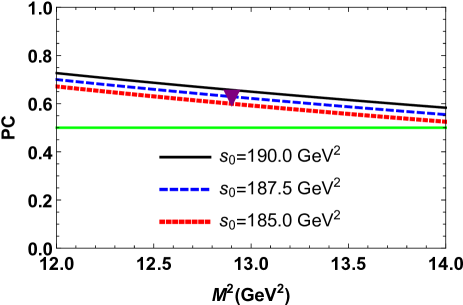
Figure 1: The pole contribution $\mathrm{PC}$ vs the Borel parameter $M^{2}$ at fixed $s_{0}$. The mass $m$ of the tetraquark $T$ has been evaluated at a position fixed by the red triangle.

Auxiliary quantities $M^{2}$ and $s_{0}$ are chosen inside of the regions

$$M^{2}\in[12,14]~{}\mathrm{GeV}^{2},\ s_{0}\in[185,190]~{}\mathrm{GeV}^{2}.$$ (12)

These working windows satisfy constraints of the sum rule computations. Thus, at $M^{2}=14~{}\mathrm{GeV}^{2}$ and $M^{2}=12~{}\mathrm{GeV}^{2}$ on the average in $s_{0}$ the pole contribution ($\mathrm{PC}$)

$$\mathrm{PC}=\frac{\Pi(M^{2},s_{0})}{\Pi(M^{2},\infty)},$$ (13)

is $\mathrm{PC}\approx 0.55$ and $\mathrm{PC}$ $\approx 0.7$, respectively (Fig. 1). At $M^{2}=12~{}\mathrm{GeV}^{2}$ the nonperturbative term is positive and forms less than $1\%$ of $\Pi(M^{2},s_{0})$.

The quantities $m$ and $\Lambda$ are estimated as mean values of these parameters over the regions Eq. (12)

$$m = (12795\pm 90)~{}\mathrm{MeV},$$

$$\Lambda = (2.51\pm 0.28)~{}\mathrm{GeV}^{5}.$$ (14)

The predictions Eq. (14) are equal to SR results at $M^{2}=12.9~{}\mathrm{GeV}^{2}$ and $s_{0}=187.5~{}\mathrm{GeV}^{2}$. At this point the pole contribution is equal to $0.63$, which ensures the dominance of $\mathrm{PC}$ and demonstrates ground-level nature of $T$. The mass $m$ of the tetraquark $T$ as function of the parameters $M^{2}$ and $s_{0}$ is depicted in Fig. 2.

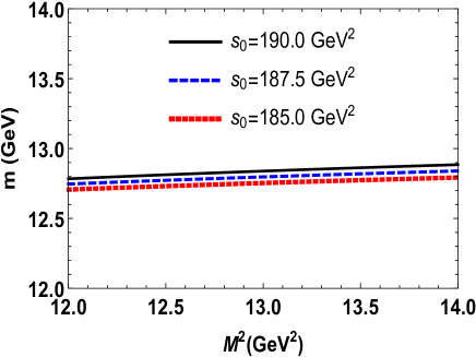
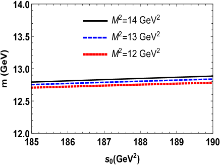
Figure 2: Dependence of the mass $m$ on the Borel $M^{2}$ (left panel), and continuum threshold $s_{0}$ parameters (right panel).

The mass of the four-quark tensor structures $bb\overline{c}\overline{c}$/$cc\overline{b}\overline{b}$ was calculated in the context of various methods. Thus, using a nonrelativistic quark model the authors of Ref. Wang:2019rdo found that the minimal  mass of the state $bb\overline{c}\overline{c}$ is around of $12868~{}\mathrm{MeV}$. It is interesting that in the relativistic quark model the mass of such lowest-level tensor tetraquark was estimated $12859~{}\mathrm{MeV}$ Galkin:2023wox . Within uncertainties of computations these results are consistent with our prediction.

The molecule and tetraquark states $bb\overline{c}\overline{c}$ were considered in Ref. Chen:2019vrj in a nonrelativistic chiral quark model. Calculations carried out there suggest that no bound state can be formed for $bb\overline{c}\overline{c}$ and $bc\overline{b}\overline{c}$ systems. The mass spectra of different all-heavy tetraquarks including $bb\overline{c}\overline{c}$/$cc\overline{b}\overline{b}$ ones were explored in Ref. Liu:2019zuc , as well. In this article, analysis was performed in the framework of the potential model which includes the linear confining potential, Coulomb potential, and spin-spin interactions. It was demonstrated that the tensor tetraquark $bb\overline{c}\overline{c}$ has the mass equal to $12972~{}\mathrm{MeV}$. This estimate is slightly higher than our result but is, qualitatively, in accord with all samples considered till now. In other words, in these papers the exotic tensor meson $bb\overline{c}\overline{c}$ was found unstable against strong decays. Only in some publications, in Ref. Wang:2021taf for instance, this tensor tetraquark has the mass $12.37_{-0.16}^{+0.19}~{}\mathrm{GeV}$ and is strong-interaction stable structure.

Our result for $m$ implies that it is above the $B_{c}B_{c}$, $B_{c}B_{c}^{\ast}$, and $B_{c}^{\ast}B_{c}^{\ast}$ thresholds $12.55~{}\mathrm{GeV}$, $12.62~{}\mathrm{GeV}$ and $12.68~{}\mathrm{GeV}$ and can decay to these final states. In the next sections, we are going to calculate partial widths of these processes, and estimate full width of the tensor tetraquark $bb\overline{c}\overline{c}$.

III Decay $T\rightarrow B_{c}^{-}B_{c}^{-}$

We start from analysis of the process $T\rightarrow B_{c}^{-}B_{c}^{-}$. The width of this decay can be computed using the strong coupling $g$ of particles at the vertex $TB_{c}^{-}B_{c}^{-}$. In order to find $g$ it is convenient to analyze the three-point correlation function

$$\Pi_{\mu\nu}(p,p^{\prime}) = i^{2}\int d^{4}xd^{4}ye^{ip^{\prime}y}e^{-ipx}\langle 0|\mathcal{T}\{J^{B_{c}}(y)$$ (15)

$$\times J^{B_{c}}(0)J_{\mu\nu}^{\dagger}(x)\}|0\rangle,$$

where

$$J^{B_{c}}(x)=\overline{c}_{i}(x)i\gamma_{5}b_{i}(x),$$ (16)

is the interpolating current of the pseudoscalar meson $B_{c}^{-}$.

Investigation of the correlation function $\Pi_{\mu\nu}(p,p^{\prime})$ makes it possible to derive the SR for the form factor $g(q^{2})$ that at the mass shell $q^{2}=m_{B_{c}}^{2}$ is equal to the strong coupling $g$. To find SR for the form factor $g(q^{2})$, we first write down $\Pi_{\mu\nu}(p,p^{\prime})$ using the parameters of the tetraquark $T$ and meson $B_{c}^{-}$. The correlation function $\Pi_{\mu\nu}^{\mathrm{Phys}}(p,p^{\prime})$ calculated by this method forms the physical side of the SR for the form factor $g_{1}(q^{2})$ and is given by the formula

$$\Pi_{\mu\nu}^{\mathrm{Phys}}(p,p^{\prime})=\frac{\langle 0|J^{B_{c}}|B_{c}(p^{\prime})\rangle}{p^{\prime 2}-m_{B_{c}}^{2}}\frac{\langle 0|J^{B_{c}}|B_{c}(q)\rangle}{q^{2}-m_{B_{c}}^{2}}$$

$$\times\langle B_{c}(p^{\prime})B_{c}(q)|T(p,\varepsilon)\rangle\frac{\langle T(p,\varepsilon)|J_{\mu\nu}^{\dagger}|0\rangle}{p^{2}-m^{2}}+\cdots,$$

(17)

with $m_{B_{c}}=(6274.47\pm 0.27)~{}\mathrm{MeV}$ being the mass of $B_{c}^{-}$ meson PDG:2022 . The correlation function $\Pi_{\mu\nu}^{\mathrm{Phys}}(p,p^{\prime})$ is found after isolating an effect of the ground-level particles, whereas contributions of higher and continuum states are denoted by the ellipses. To recast this correlator into a form suitable for further analysis, we use the matrix element

$$\langle 0|J^{B_{c}}|B_{c}\rangle=\frac{f_{B_{c}}m_{B_{c}}^{2}}{m_{b}+m_{c}},$$ (18)

where $f_{B_{c}}=(476\pm 27)~{}\mathrm{MeV}$ is the decay constant of the mesons $B_{c}^{\pm}$ Veliev:2010vd . We model the vertex of the tensor tetraquark and two pseudoscalar mesons by the formula

$$\langle B_{c}(p^{\prime})B_{c}(q)|T(p,\varepsilon)\rangle=-g(q^{2})\varepsilon_{\alpha\beta}^{(\lambda)}(p)p^{\prime\alpha}q^{\beta},$$ (19)

with $g(q^{2})$ being the strong form factor that at the mass shell $q^{2}=m_{B_{c}}^{2}$ determines the coupling $g$ of interest. By taking into account $q=p-p^{\prime}$ and

$$\varepsilon_{\alpha\beta}^{(\lambda)}(p)p^{\alpha}=\varepsilon_{\alpha\beta}^{(\lambda)}(p)p^{\beta}=0,$$ (20)

we get

$$\langle B_{c}(p^{\prime})B_{c}(q)|T(p,\varepsilon)\rangle=g(q^{2})\varepsilon_{\alpha\beta}^{(\lambda)}(p)p^{\prime\alpha}p^{\prime\beta}.$$ (21)

For the correlator, we find

$$\Pi_{\mu\nu}^{\mathrm{Phys}}(p,p^{\prime})=\frac{g(q^{2})\Lambda f_{B_{c}}^{2}m_{B_{c}}^{4}}{(m_{b}+m_{c})^{2}\left(p^{2}-m^{2}\right)(p^{\prime 2}-m_{B_{c}}^{2})}$$

$$\times\frac{1}{(q^{2}-m_{B_{c}}^{2})}\left\{\frac{\lambda^{2}}{3}g_{\mu\nu}+\left[\frac{m_{B_{c}}^{2}}{m^{2}}+\frac{2\lambda^{2}}{3m^{2}}\right]p_{\mu}p_{\nu}\right.$$

$$\left.+p_{\mu}^{\prime}p_{\nu}^{\prime}-\frac{m^{2}+m_{B_{c}}^{2}-q^{2}}{2m^{2}}(p_{\mu}p_{\nu}^{\prime}+p_{\nu}p_{\mu}^{\prime})\right\},$$ (22)

where $\lambda=\lambda(m,m_{B_{c}},q)$ and

$$\lambda(x,y,z)=\frac{\sqrt{x^{4}+y^{4}+z^{4}-2(x^{2}y^{2}+x^{2}z^{2}+y^{2}z^{2})}}{2x}.$$ (23)

The correlation function $\Pi_{\mu\nu}^{\mathrm{Phys}}(p,p^{\prime})$ has the structure

$$\Pi_{\mu\nu}^{\mathrm{Phys}}(p,p^{\prime})=\Pi_{0}^{\mathrm{Phys}}g_{\mu\nu}+\Pi_{1}^{\mathrm{Phys}}p_{\mu}p_{\nu}+\Pi_{2}^{\mathrm{Phys}}p_{\mu}^{\prime}p_{\nu}^{\prime}$$

$$+\Pi_{3}^{\mathrm{Phys}}p_{\mu}p_{\nu}^{\prime}+\Pi_{4}^{\mathrm{Phys}}p_{\nu}p_{\mu}^{\prime}.$$ (24)

The amplitudes $\Pi_{i}^{\mathrm{Phys}}$ are functions of the variables $p^{2},p^{\prime 2},q^{2}$, and depend on the parameters $m^{2}$ and $m_{B_{c}}^{2}$ which are omitted for compactness of the expression. To derive the SR for the form factor $g(q^{2})$, we work with the structure $p_{\mu}^{\prime}p_{\nu}^{\prime}$ and corresponding invariant amplitude $\Pi^{\mathrm{Phys}}(p^{2},p^{\prime 2},q^{2})$ (we have omitted a subscript $2$). It has the form

$$\Pi^{\mathrm{Phys}}(p^{2},p^{\prime 2},q^{2})=\frac{g(q^{2})\Lambda f_{B_{c}}^{2}m_{B_{c}}^{4}}{(m_{b}+m_{c})^{2}\left(p^{2}-m^{2}\right)}$$

$$\times\frac{1}{(p^{\prime 2}-m_{B_{c}}^{2})(q^{2}-m_{B_{c}}^{2})}.$$ (25)

The QCD side of the sum rule, i.e., the correlation function $\Pi_{\mu\nu}^{\mathrm{OPE}}(p,p^{\prime})$ is determined by the formula

$$\Pi_{\mu\nu}^{\mathrm{OPE}}(p,p^{\prime})=2i^{2}\int d^{4}xd^{4}ye^{ip^{\prime}y}e^{-ipx}\left\{\mathrm{Tr}\left[\gamma_{5}S_{b}^{ia}(y-x)\right.\right.$$

$$\left.\times\gamma_{\nu}\widetilde{S}_{b}^{jb}(-x)\gamma_{5}\widetilde{S}_{c}^{aj}(x)\gamma_{\mu}S_{c}^{bi}(x-y)\right]$$

$$\left.-\mathrm{Tr}\left[\gamma_{5}S_{b}^{ia}(y-x)\gamma_{\nu}\widetilde{S}_{b}^{jb}(-x)\gamma_{5}\widetilde{S}_{c}^{bj}(x)\gamma_{\mu}S_{c}^{ai}(x-y)\right]\right\}.$$

(26)

The correlator $\Pi_{\mu\nu}^{\mathrm{OPE}}(p,p^{\prime})$ has the same Lorentz structure as $\Pi_{\mu\nu}^{\mathrm{Phys}}$. We label by $\Pi^{\mathrm{OPE}}(p^{2},p^{\prime 2},q^{2})$ the amplitude of the structure $p_{\mu}^{\prime}p_{\nu}^{\prime}$ and employ it in the following analysis. Having equated functions $\Pi^{\mathrm{Phys}}(p^{2},p^{\prime 2},q^{2})$ and $\Pi^{\mathrm{OPE}}(p^{2},p^{\prime 2},q^{2})$, and fulfilled the Borel transformations over variables $-p^{2}$ and $-p^{\prime 2}$ and continuum subtraction procedures, we find

$$g(q^{2})=\frac{(m_{b}+m_{c})^{2}}{\Lambda f_{B_{c}}^{2}m_{B_{c}}^{4}}(q^{2}-m_{B_{c}}^{2})$$

$$\times e^{m^{2}/M_{1}^{2}}e^{m_{B_{c}}^{2}/M_{2}^{2}}\Pi(\mathbf{M}^{2},\mathbf{s}_{0},q^{2}),$$ (27)

where

$$\Pi(\mathbf{M}^{2},\mathbf{s}_{0},q^{2})=\int_{4\mathcal{M}^{2}}^{s_{0}}ds\int_{\mathcal{M}^{2}}^{s_{0}^{\prime}}ds^{\prime}\rho(s,s^{\prime},q^{2})$$

$$\times e^{-s/M_{1}^{2}}e^{-s^{\prime}/M_{2}^{2}},$$ (28)

and $\mathcal{M}=m_{b}+m_{c}$. Here, $\Pi(\mathbf{M}^{2},\mathbf{s}_{0},q^{2})$ is the Borel transformed and continuum subtracted amplitude $\Pi^{\mathrm{OPE}}(p^{2},p^{\prime 2},q^{2})$ corresponding to the term $\sim p_{\mu}^{\prime}p_{\nu}^{\prime}$. The spectral density $\rho(s,s^{\prime},q^{2})$ is calculated as a imaginary part of the component $\sim p_{\mu}^{\prime}p_{\nu}^{\prime}$ in the correlation function. The $(\mathbf{M}^{2},\mathbf{s}_{0})$ in Eq. (28) are two pairs of the parameters: The parameters $(M_{1}^{2},s_{0})$ corresponds to the tensor tetraquark channel, and in numerical analysis we use Eq. (12). The pair $(M_{2}^{2},s_{0}^{\prime})$ describes the $B_{c}^{-}$ channel for which we employ

$$M_{2}^{2}\in[6.5,7.5]~{}\mathrm{GeV}^{2},\ s_{0}^{\prime}\in[45,47]~{}\mathrm{GeV}^{2}.$$ (29)

The strong coupling $g$ is equal to the form factor $g(m_{B_{c}}^{2})$ computed at the mass shell $q^{2}=m_{B_{c}}^{2}$. Because the SR method is applicable only in the domain $q^{2}<0$, to get $g(m_{B_{c}}^{2})$ one has to extrapolate the QCD numerical data to a region of positive $q^{2}$. For these purposes, it is appropriate to use a variable $Q^{2}=-q^{2}$, and denote the fit function $\mathcal{F}(Q^{2})$, which at $Q^{2}>0$ gives results equal to SR data, but can be easily extrapolated to $Q^{2}<0$. One of possible choices for the such function is

$$\mathcal{F}(Q^{2})=\mathcal{F}^{0}\mathrm{\exp}\left[c_{1}\frac{Q^{2}}{m^{2}}+c_{2}\left(\frac{Q^{2}}{m^{2}}\right)^{2}\right].$$ (30)

This function contains the unknown parameters $\mathcal{F}^{0}$, $c_{1}$, and $c_{2}$ which should be determined from a fitting procedure.

We carry out the numerical computations varying $Q^{2}$ inside of the interval $Q^{2}=1-40~{}\mathrm{GeV}^{2}$. The QCD data extracted from the SR analysis for the form factor $|g(Q^{2})|$ are plotted in Fig. 3. Having compared these data and Eq. (30), one can obtain the parameters $\mathcal{F}^{0}=21.44~{}\mathrm{GeV}^{-1}$, $c_{1}=1.18$, and $c_{2}=2.21$ of the function $\mathcal{F}(Q^{2})$. This function is plotted in Fig. 3 as well: A reasonable agreement between $\mathcal{F}(Q^{2})$ and QCD data is evident.

For the strong coupling $g$, we find

$$|g|\equiv\mathcal{F}(-m_{B_{c}}^{2})=(18.33\pm 2.02)\ \mathrm{GeV}^{-1}.$$ (31)

The partial width of the decay $T\rightarrow B_{c}^{-}B_{c}^{-}$ is determined by the following formula

$$\Gamma\left[T\rightarrow B_{c}^{-}B_{c}^{-}\right]=\frac{g^{2}\lambda}{2\cdot 960\pi m^{2}}\left(m^{2}-2m_{B_{c}}^{2}\right)^{2},$$ (32)

where $\lambda=\lambda(m,m_{B_{c}},m_{B_{c}})$. Having applied Eqs. (31) and (32) and other input parameters, we get the partial width of this decay

$$\Gamma\left[T\rightarrow B_{c}^{-}B_{c}^{-}\right]=(16.3\pm 3.8)~{}\mathrm{MeV}.$$ (33)

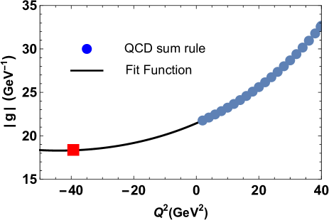
Figure 3: The QCD data for the form factor $|g(Q^{2})|$ and the extrapolating function $\mathcal{F}$. The red square shows the point $Q^{2}=-m_{B_{c}}^{2}$.

IV Decay $T\rightarrow B_{c}^{-}B_{c}^{\ast-}$

Here, we study the process $T\rightarrow B_{c}^{-}B_{c}^{\ast-}$ and calculate its partial width. To this end, we begin from analysis of the correlation function

$$\Pi_{\alpha\mu\nu}(p,p^{\prime}) = i^{2}\int d^{4}xd^{4}ye^{ip^{\prime}y}e^{-ipx}\langle 0|\mathcal{T}\{J_{\alpha}^{B_{c}^{\ast}}(y)$$ (34)

$$\times J^{B_{c}}(0)J_{\mu\nu}^{\dagger}(x)\}|0\rangle,$$

which is necessary to evaluate the strong coupling at the vertex $TB_{c}B_{c}^{\ast}$. In Eq. (34) $J_{\mu}^{B_{c}^{\ast}}(y)$ is the interpolating current of the vector meson $B_{c}^{\ast-}$

$$J_{\mu}^{B_{c}^{\ast}}(y)=\overline{c}_{i}(x)\gamma_{\mu}b_{i}(x).$$ (35)

The SR investigation requires calculation the correlator $\Pi_{\alpha\mu\nu}(p,p^{\prime})$ in two regions. First, one should find it using the physical parameters of particles involved into the decay process. This expression which contains contribution of only ground-state particles is

$$\Pi_{\alpha\mu\nu}^{\mathrm{Phys}}(p,p^{\prime})=\frac{\langle 0|J_{\alpha}^{B_{c}^{\ast}}|B_{c}^{\ast}(p^{\prime},\epsilon)\rangle}{p^{\prime 2}-m_{B_{c}^{\ast}}^{2}}\frac{\langle 0|J^{B_{c}}|B_{c}(q)\rangle}{q^{2}-m_{B_{c}}^{2}}$$

$$\times\langle B_{c}^{\ast}(p^{\prime},\epsilon)B_{c}(q)|T(p,\varepsilon)\rangle\frac{\langle T(p,\varepsilon)|J_{\mu\nu}^{\dagger}|0\rangle}{p^{2}-m^{2}}+\cdots.$$

(36)

The matrix element of the vector particle is

$$\langle 0|J_{\mu}^{B_{c}^{\ast}}|B_{c}^{\ast}(p)\rangle=f_{B_{c}^{\ast}}m_{B_{c}^{\ast}}\epsilon_{\mu}(p),$$ (37)

where $m_{B_{c}^{\ast}}$ and $f_{B_{c}^{\ast}}$ are the mass and decay constant of the meson $B_{c}^{\ast}(p)$, respectively. The vertex $TB_{c}B_{c}^{\ast}$ is modeled by the formula

$$\langle B_{c}^{\ast}(p^{\prime},\epsilon)B_{c}(q)|T(p,\varepsilon)\rangle=h(q^{2})\varepsilon_{\beta\tau\rho\delta}p^{\beta}\varepsilon_{(\lambda)}^{\tau\sigma}(p)q_{\sigma}p^{\prime\rho}{}\epsilon^{\ast\delta}.$$ (38)

Having substituted these matrix elements in Eq. (36), we get

$$\Pi_{\alpha\mu\nu}^{\mathrm{Phys}}(p,p^{\prime})=\frac{h(q^{2})\Lambda f_{B_{c}^{\ast}}m_{B_{c}^{\ast}}f_{B_{c}}m_{B_{c}}^{2}}{2(m_{b}+m_{c})\left(p^{2}-m^{2}\right)(p^{\prime 2}-m_{B_{c}^{\ast}}^{2})}$$

$$\times\frac{1}{(q^{2}-m_{B_{c}^{\ast}}^{2})}\left\{\varepsilon_{\lambda\beta\alpha\mu}p^{\lambda}p^{\prime\beta}p_{\nu}^{\prime}+\varepsilon_{\lambda\beta\alpha\nu}p^{\lambda}p^{\prime\beta}p_{\mu}^{\prime}\right.$$

$$\left.-\frac{m^{2}+m_{B_{c}^{\ast}}^{2}-q^{2}}{2m^{2}}\left(\varepsilon_{\lambda\beta\alpha\nu}p^{\lambda}p^{\prime\beta}p_{\mu}+\varepsilon_{\lambda\beta\alpha\mu}p^{\lambda}p^{\prime\beta}p_{\nu}\right)\right\}.$$

(39)

The QCD side of the sum rule is determined by the expression

$$\Pi_{\alpha\mu\nu}^{\mathrm{OPE}}(p,p^{\prime})=2i\int d^{4}xd^{4}ye^{ip^{\prime}y}e^{-ipx}\left\{\mathrm{Tr}\left[\gamma_{\alpha}S_{b}^{ia}(y-x)\right.\right.$$

$$\left.\times\gamma_{\nu}\widetilde{S}_{b}^{jb}(-x)\gamma_{5}\widetilde{S}_{c}^{aj}(x)\gamma_{\mu}S_{c}^{bi}(x-y)\right]$$

$$\left.-\mathrm{Tr}\left[\gamma_{\alpha}S_{b}^{ia}(y-x)\gamma_{\nu}\widetilde{S}_{b}^{jb}(-x)\gamma_{5}\widetilde{S}_{c}^{bj}(x)\gamma_{\mu}S_{c}^{ai}(x-y)\right]\right\}.$$

(40)

We derive SR for the form factor $h(q^{2})$ using the first structure in Eq. (39) and its counterpart in $\Pi_{\alpha\mu\nu}^{\mathrm{OPE}}(p,p^{\prime})$

$$h(q^{2}) = \frac{2(m_{b}+m_{c})(q^{2}-m_{B_{c}^{\ast}}^{2})}{\Lambda f_{B_{c}^{\ast}}m_{B_{c}^{\ast}}f_{B_{c}}m_{B_{c}}^{2}}$$ (41)

$$\times e^{m^{2}/M_{1}^{2}}e^{m_{B_{c}^{\ast}}^{2}/M_{2}^{2}}\widehat{\Pi}(\mathbf{M}^{2},\mathbf{s}_{0},q^{2}),$$

where $\widehat{\Pi}(\mathbf{M}^{2},\mathbf{s}_{0},q^{2})$ is the amplitude corresponding to the structure $\varepsilon_{\lambda\beta\alpha\mu}p^{\lambda}p^{\prime\beta}p_{\nu}^{\prime}$ in the correlation function $\Pi_{\alpha\mu\nu}^{\mathrm{OPE}}(p,p^{\prime})$ after the Borel transformations and continuum subtractions.

In numerical computations, we utilize the theoretical predictions for the mass and decay constant of the vector meson $B_{c}^{\ast}$

$$m_{B_{c}^{\ast}}=6338~{}\mathrm{MeV,\ }\,f_{B_{c}^{\ast}}=471~{}\mathrm{MeV}$$ (42)

from Refs. Godfrey:2004ya ; Eichten:2019gig , respectively. The parameters in the $B_{c}^{\ast}$ channel are chosen in accordance with Eq. (43):

$$M_{2}^{2}\in[6.5,7.5]~{}\mathrm{GeV}^{2},\ s_{0}^{\prime}\in[49,51]~{}\mathrm{GeV}^{2}.$$ (43)

The results of numerical analysis for $h(q^{2})$ and extrapolating function $\widehat{\mathcal{F}}(Q^{2})$ with parameters $\widehat{\mathcal{F}}^{0}=1.67~{}\mathrm{GeV}^{-2}$, $c_{1}=1.26$, and $c_{2}=1.95$ are drawn in Fig. 4.

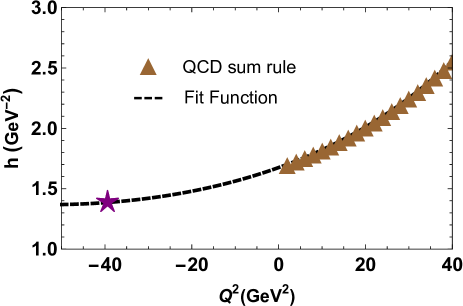
Figure 4: The SR output and interpolating function for the form factor $h(Q^{2})$. The star shows the point $Q^{2}=-m_{B_{c}}^{2}$.

Having employed the fit function $\widehat{\mathcal{F}}(Q^{2})$, it is not difficult to estimate the strong coupling $h$

$$h\equiv\widehat{\mathcal{F}}(-m_{B_{c}^{\ast}}^{2})=(1.39\pm 0.15)\ \mathrm{GeV}^{-2}.$$ (44)

The partial width of the decay $T\rightarrow B_{c}^{-}B_{c}^{\ast-}$ is equal to

$$\Gamma\left[T\rightarrow B_{c}^{-}B_{c}^{\ast-}\right] = \frac{h^{2}\widehat{\lambda}}{640\pi m^{4}}\left[m_{B_{c}}^{4}+(m^{2}-m_{B_{c}^{\ast}}^{2})^{2}\right.,$$ (45)

$$\left.-2m_{B_{c}}^{2}(m^{2}+m_{B_{c}^{\ast}}^{2})\right]^{2},$$

where $\widehat{\lambda}=\lambda(m,m_{B_{c}^{\ast}},m_{B_{c}})$. Having applied Eqs. (44) and (45) and other input parameters, we evaluate the partial width of this process

$$\Gamma\left[T\rightarrow B_{c}^{-}B_{c}^{\ast-}\right]=(25.2\pm 6.9)~{}\mathrm{MeV}.$$ (46)

V Decay $T\rightarrow B_{c}^{\ast-}B_{c}^{\ast-}$

In the case of the decay $T\rightarrow B_{c}^{\ast-}B_{c}^{\ast-}$ the SR for the strong form factor $G(q^{2})$ at the vertex $TB_{c}^{\ast}B_{c}^{\ast}$ can be obtained from the correlation function

$$\Pi_{\alpha\beta\mu\nu}(p,p^{\prime}) = i^{2}\int d^{4}xd^{4}ye^{ip^{\prime}y}e^{-ipx}\langle 0|\mathcal{T}\{J_{\alpha}^{B_{c}^{\ast}}(y)$$ (47)

$$\times J_{\beta}^{B_{c}^{\ast}}(0)J_{\mu\nu}^{\dagger}(x)\}|0\rangle.$$

The correlation function $\Pi_{\alpha\beta\mu\nu}(p,p^{\prime})$ can be expressed using the physical parameters of the particles involved onto the decay process

$$\Pi_{\alpha\beta\mu\nu}^{\mathrm{Phys}}(p,p^{\prime})=\frac{\langle 0|J_{\alpha}^{B_{c}^{\ast}}|B_{c}^{\ast}(p^{\prime},\epsilon_{1})\rangle}{p^{\prime 2}-m_{B_{c}^{\ast}}^{2}}\frac{\langle 0|J_{\beta}^{B_{c}^{\ast}}|B_{c}^{\ast}(q,\epsilon_{2})\rangle}{q^{2}-m_{B_{c}^{\ast}}^{2}}$$

$$\times\langle B_{c}^{\ast}(p^{\prime},\epsilon_{1})B_{c}^{\ast}(q,\epsilon_{2})|T(p,\varepsilon)\rangle\frac{\langle T(p,\varepsilon)|J_{\mu\nu}^{\dagger}|0\rangle}{p^{2}-m^{2}}+\cdots,$$

where $\epsilon_{1\mu}$ and $\epsilon_{2\mu}$ are the polarization vector of the $B_{c}^{\ast}$ mesons with momenta $p^{\prime}$ and $q$, respectively. In the correlator $\Pi_{\alpha\beta\mu\nu}^{\mathrm{Phys}}(p,p^{\prime})$ only contribution of the ground-level particles is presented explicitly: Contributions arising from the higher resonances and continuum states are shown by the dots.

The correlation function can be further simplified using the matrix element of the vertex $\langle B_{c}^{\ast}(p^{\prime},\epsilon_{1})B_{c}^{\ast}(q,\epsilon_{2})|T(p,\varepsilon)\rangle$. In general, a tensor-vector-vector vertex contains three independent form factors which describe a pair of vector meson with helicities $\lambda=0$, $\pm 1$ and $\pm 2$ Braun:2000cs ; Aliev:2018kry . In the case of two photon decays of a tensor meson it was argued that a dominant contribution comes from a $\lambda=2$ state Singer:1983bu . In the present work, we assume that this conclusion may be applied to decay $T\rightarrow B_{c}^{\ast-}B_{c}^{\ast-}$, as well, and choose the vertex in the form

$$\langle B_{c}^{\ast}(p^{\prime},\epsilon_{1})B_{c}^{\ast}(q,\epsilon_{2})|T(p,\varepsilon)\rangle=G(q^{2})\varepsilon_{\tau\rho}^{(\lambda)}\left[(\epsilon_{1}^{\ast}\cdot q)\epsilon_{2}^{\tau\ast}p^{\prime\rho}\right.$$

$$\left.+(\epsilon_{2}^{\ast}\cdot p^{\prime})\epsilon_{1}^{\ast\tau}q^{\rho}-(p^{\prime}\cdot q)\epsilon_{1}^{\tau\ast}\epsilon_{2}^{\rho\ast}-(\epsilon_{1}^{\ast}\cdot\epsilon_{2}^{\ast})p^{\prime\tau}q^{\rho}\right],$$

(49)

which corresponds to a pure $\lambda=2$ final state.

As a result, for $\Pi_{\alpha\beta\mu\nu}^{\mathrm{Phys}}(p,p^{\prime})$ we get the lengthy expression

$$\Pi_{\alpha\beta\mu\nu}^{\mathrm{Phys}}(p,p^{\prime})=\frac{G(q^{2})\Lambda f_{B_{c}^{\ast}}^{2}m_{B_{c}^{\ast}}^{2}}{\left(p^{2}-m^{2}\right)(p^{\prime 2}-m_{B_{c}^{\ast}}^{2})(q^{2}-m_{B_{c}^{\ast}}^{2})}$$

$$\times\left\{\frac{m_{B_{c}^{\ast}}^{4}-2m_{B_{c}^{\ast}}^{2}(2m^{2}+q^{2})+(m^{2}-q^{2})(3m^{2}-q^{2})}{12m^{2}}\right.$$

$$\times g_{\mu\nu}g_{\alpha\beta}+\frac{1}{3}g_{\mu\nu}\left(\frac{m_{B_{c}^{\ast}}^{2}}{m^{2}}p_{\alpha}p_{\beta}+2p_{\alpha}^{\prime}p_{\beta}^{\prime}\right)-\frac{1}{6m^{2}}g_{\mu\nu}$$

$$\times\left[(m_{B_{c}^{\ast}}^{2}+3m^{2}-q^{2})p_{\alpha}p_{\beta}^{\prime}+(m_{B_{c}^{\ast}}^{2}+m^{2}-q^{2})p_{\alpha}^{\prime}p_{\beta}\right]$$

$$+\frac{1}{2}p_{\alpha}p_{\mu}^{\prime}g_{\beta\nu}+\frac{1}{2m^{2}}\left(p_{\beta}p_{\nu}p_{\alpha}^{\prime}p_{\mu}^{\prime}+p_{\beta}p_{\mu}p_{\alpha}^{\prime}p_{\nu}^{\prime}\right)$$

$$\left.+\text{other structures}\right\}.$$ (50)

For the QCD side of the sum rule, we obtain

$$\Pi_{\alpha\beta\mu\nu}^{\mathrm{OPE}}(p,p^{\prime})=2i^{2}\int d^{4}xd^{4}ye^{ip^{\prime}y}e^{-ipx}\left\{\mathrm{Tr}\left[\gamma_{\alpha}S_{b}^{ia}(y-x)\right.\right.$$

$$\left.\times\gamma_{\nu}\widetilde{S}_{b}^{jb}(-x)\gamma_{\beta}\widetilde{S}_{c}^{aj}(x)\gamma_{\mu}S_{c}^{bi}(x-y)\right]$$

$$\left.-\mathrm{Tr}\left[\gamma_{\alpha}S_{b}^{ia}(y-x)\gamma_{\nu}\widetilde{S}_{b}^{jb}(-x)\gamma_{\beta}\widetilde{S}_{c}^{bj}(x)\gamma_{\mu}S_{c}^{ai}(x-y)\right]\right\}.$$

(51)

To get the required SR for the form factor $G(q^{2})$ we utilize the structure proportional to $p_{\alpha}p_{\mu}^{\prime}g_{\beta\nu}$ and corresponding amplitudes $\widetilde{\Pi}^{\mathrm{Phys}}(p^{2},p^{\prime 2},q^{2})$ and $\widetilde{\Pi}^{\mathrm{OPE}}(p^{2},p^{\prime 2},q^{2})$ in both versions of the correlation function $\Pi_{\alpha\beta\mu\nu}(p,p^{\prime})$. Then, after standard operations the sum rule for $G(q^{2})$ reads

$$G(q^{2})=\frac{2(q^{2}-m_{B_{c}^{\ast}}^{2})}{\Lambda f_{B_{c}^{\ast}}^{2}m_{B_{c}^{\ast}}^{2}}e^{m^{2}/M_{1}^{2}}e^{m_{B_{c}^{\ast}}^{2}/M_{2}^{2}}\widetilde{\Pi}(\mathbf{M}^{2},\mathbf{s}_{0},q^{2}).$$ (52)

The results obtained for $G(Q^{2})$ are plotted in Fig. 5, where $Q^{2}$ varies inside of limits $Q^{2}=1-40~{}\mathrm{GeV}^{2}$. Then, having confronted QCD output and Eq. (30), it is easy to find $\widetilde{\mathcal{F}}^{0}=0.50~{}\mathrm{GeV}^{-1}$, $c_{1}=1.77$, and $c_{2}=-2.39$ in the function $\widetilde{\mathcal{F}}(Q^{2})$. It is also plotted in Fig. 5, where one sees a nice agreement of $\widetilde{\mathcal{F}}(Q^{2})$ and QCD data.

For the strong coupling $G$, we find

$$G\equiv\widetilde{\mathcal{F}}(-m_{B_{c}^{\ast}}^{2})=(2.8\pm 0.3)\times 10^{-1}\ \mathrm{GeV}^{-1}.$$ (53)

The partial width of the decay $T\rightarrow B_{c}^{\ast-}B_{c}^{\ast-}$ is determined by the expression

$$\Gamma\left[T\rightarrow B_{c}^{\ast-}B_{c}^{\ast-}\right]=\frac{G^{2}\widetilde{\lambda}}{2\cdot 80\pi m^{2}}\left(m^{4}-3m^{2}m_{B_{c}^{\ast}}^{2}+6m_{B_{c}^{\ast}}^{4}\right),$$ (54)

with $\widetilde{\lambda}$ being equal to $\lambda(m,m_{B_{c}^{\ast}},m_{B_{c}^{\ast}})$. As a result, we find

$$\Gamma\left[T\rightarrow B_{c}^{\ast-}B_{c}^{\ast-}\right]=(14.0\pm 3.6)~{}\mathrm{MeV}.$$ (55)

The full width of the tetraquark $T$ saturated by these three decay channels is

$$\Gamma_{\mathrm{T}}=(55.5\pm 8.7)~{}\mathrm{MeV}.$$ (56)

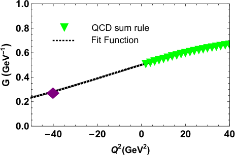
Figure 5: The QCD data for the form factor $G(Q^{2})$ and fit function $\widetilde{\mathcal{F}}$. The diamond fixes the point $Q^{2}=-m_{B_{c}}^{\ast 2}$.

VI Summary

In present paper we have studied, in a rather detailed form, the tensor tetraquark $T=bb\overline{c}\overline{c}$ by calculating its mass, current coupling and full width. The mass of this particle is above a few two $B_{c}^{(\ast)-}B_{c}^{(\ast)-}$ meson thresholds. As a result, it is unstable against strong decays to $B_{c}^{-}B_{c}^{-}$, $B_{c}^{-}B_{c}^{\ast-}$, and $B_{c}^{\ast-}B_{c}^{\ast-}$ pairs. The full width of $T$  have been evaluated by taking into account namely these decay channels.

The prediction for the full width $\Gamma_{\mathrm{T}}=(55.5\pm 8.7)~{}\mathrm{MeV}$ of the tensor tetraquark is comparable with our results for the scalar and axial-vector tetraquarks $bb\overline{c}\overline{c}$. It is smaller than widths of the scalar tetraquarks, but larger than the width of the axial-vector state $T_{\mathrm{1}}$. In any case, parameters of the tensor tetraquark $T$ do not differ considerably from those of scalar and axial-vector states and fit the class of $bb\overline{c}\overline{c}$ exotic mesons.

Although spectroscopic parameters of the tetraquarks $bb\overline{c}\overline{c}$ were calculated in the context of different models and approaches, the same cannot be said for their decay channels. But it is difficult to make credible conclusions about nature of these states without information on their widths. This is very important, because there are controversial predictions in the literature concerning stability of the $bb\overline{c}\overline{c}$ particles. As is seen, there is plenty to be done for comprehensive analyses of the four-quark structures $bb\overline{c}\overline{c}$ with various spin-parities.

References

(1) R. Aaij et al. (LHCb Collaboration),
Sci. Bull. 65, 1983 (2020).
(2) E. Bouhova-Thacker (ATLAS Collaboration),
PoS ICHEP2022, 806 (2022).
(3) A. Hayrapetyan, et al. (CMS Collaboration),
arXiv:2306.07164 [hep-ex].
(4) J. R. Zhang,
Phys. Rev. D 103, 014018 (2021).
(5) R. M. Albuquerque, S. Narison,
A. Rabemananjara, D. Rabetiarivony, and G. Randriamanatrika,
Phys. Rev. D 102, 094001 (2020).
(6) B. C. Yang, L. Tang, and C. F. Qiao,
Eur. Phys. J. C 81, 324 (2021).
(7) C. Becchi, A. Giachino, L. Maiani, and
E. Santopinto,
Phys. Lett. B 806, 135495 (2020).
(8) C. Becchi, A. Giachino, L. Maiani, and
E. Santopinto, Phys. Lett. B 811, 135952 (2020).
(9) Z. G. Wang,
Nucl. Phys. B 985, 115983 (2022).
(10) R. N. Faustov, V. O. Galkin, and E. M. Savchenko,
Symmetry 14, 2504 (2022).
(11) P. Niu, Z. Zhang, Q. Wang, and M. L. Du,
Sci. Bull. 68, 800 (2023).
(12) W. C. Dong and Z. G. Wang,
Phys. Rev. D 107, 074010 (2023).
(13) G. L. Yu, Z. Y. Li, Z. G. Wang, J. Lu, and M. Yan,
Eur. Phys. J. C 83, 416 (2023).
(14) S. Q. Kuang, Q. Zhou, D. Guo, Q. H. Yang, and
L. Y. Dai,
Eur. Phys. J. C 83, 383 (2023).
(15) X. K. Dong, V. Baru, F. K. Guo, C. Hanhart, and
A. Nefediev,
Phys. Rev. Lett. 126, 132001 (2021); 127, 119901(E)
(2021).
(16) Z. R. Liang, X. Y. Wu, and D. L. Yao,
Phys. Rev. D 104, 034034 (2021).
(17) S. S. Agaev, K. Azizi, B. Barsbay, and H. Sundu,
Phys. Lett. B 844, 138089 (2023).
(18) S. S. Agaev, K. Azizi, B. Barsbay and H. Sundu,
Eur. Phys. J. Plus 138, 935 (2023).
(19) S. S. Agaev, K. Azizi, B. Barsbay, and H. Sundu,
Nucl. Phys. A 844, 122768 (2024).
(20) S. S. Agaev, K. Azizi, B. Barsbay, and H. Sundu,
Eur. Phys. J. C 83, 994 (2023).
(21) S. S. Agaev, K. Azizi, B. Barsbay, and H. Sundu,
Phys. Rev. D 109, 014006 (2024).
(22) J. Wu, Y. R. Liu, K. Chen, X. Liu, and S. L. Zhu,
Phys. Rev. D 97, 094015 (2018).
(23) G. Li, X. F. Wang, and Y. Xing,
Eur. Phys. J. C 79, 645 (2019).
(24) G. J. Wang, L. Meng, and S. L. Zhu,
Phys. Rev. D 100, 096013 (2019).
(25) M. S. Liu, Q. F. Lü, X. H. Zhang, and Q. Zhao,
Phys. Rev. D 100, 016006 (2019).
(26) X. Chen, Phys. Rev. D 100, 094009 (2019).
(27) Q. N. Wang, Z. Y. Yang, W. Chen, and H. X. Chen,
Phys. Rev. D 104, 014040 (2021).
(28) H. Mutuk, Phys. Lett. B 834, 137404 (2022).
(29) V. O. Galkin, and E. M. Savchenko,
arXiv:2310.20247 [hep-ph].
(30) S. S. Agaev, K. Azizi, B. Barsbay, and H. Sundu,
arXiv:2311.10534 [hep-ph].
(31) S. S. Agaev, K. Azizi, and H. Sundu,
Phys. Lett. B 851, 138562 (2024).
(32) M. A. Shifman, A. I. Vainshtein, and
V. I. Zakharov, Nucl. Phys. B 147, 385 (1979).
(33) M. A. Shifman, A. I. Vainshtein, and
V. I. Zakharov, Nucl. Phys. B 147, 448 (1979).
(34) S. S. Agaev, K. Azizi, and H. Sundu,
Turk. J. Phys. 44, 95 (2020).
(35) R. L. Workman et al. (Particle Data Group),
Prog. Theor. Exp. Phys. 2022, 083C01 (2022).
(36) E. V. Veliev, K. Azizi, H. Sundu, and N. Aksit,
J. Phys. G 39, 015002 (2012).
(37) S. Godfrey,
Phys. Rev. D 70, 054017 (2004).
(38) E. J. Eichten, and C. Quigg,
Phys. Rev. D 99, 054025 (2019).
(39) V. M. Braun, and N. Kivel,
Phys. Lett. B 501, 48 (2001).
(40) T. M. Aliev, and M. Savcı,
Phys. Rev. D 99, 015020 (2019).