Optical absorption signatures of superconductors driven by Van Hove singularities

Abstract

Due to the diverging density of states (DOS), Van Hove singularities (VHS) near the Fermi level are known to boost the susceptibility to a wide variety of electronic instabilities, including superconductivity. We theoretically show that the number of VHS in the normal state can be qualitatively inferred from the optical absorption spectra Re $\sigma_{ii}(\omega)$ in the superconducting state. The key feature is the absorption peak at frequency $\omega=2\Delta$ from the optical transition across the superconducting gap $\Delta$, which is forbidden in a single-band clean superconductor when the inversion symmetry is preserved and the band is quadratic. Although VHS dispersions are mostly quadratic, we find that a divergent peak occurs when there are multiple VHS on the Fermi surface under an applied current. In contrast, we find non-diverging weak peaks when there is only a single VHS. Depending on whether this single VHS has logarithmically or power-law divergent DOS, the peaks in Re $\sigma_{xx}(\omega)$ and Re $\sigma_{yy}(\omega)$ are nearly isotropic and anisotropic, respectively. Therefore, we propose that experimentally measured peak magnitude and anisotropy in the optical absorption spectra of VH-driven superconductors can be used to determine the number and type of VHS on the Fermi surface. Disorders could even facilitate in distinguishing the multiple and single VHS scenarios since only the diverging peak in the latter case is expected to survive.

Introduction — Van Hove singularities (VHS) are saddle points in electronic structures [1, 2], which can often be found near the Fermi level in Van der Waals materials, such as Kagome metals [3, 4, 5, 6, 7, 8, 9, 10, 11, 12, 13, 14, 15], various Moire superlattices [16, 17, 18, 19, 20, 21, 22, 23], and graphene-based few-layers heterostructure [24, 25, 26, 27, 28, 29, 30, 31, 32, 33, 34, 35, 36, 37, 38]. Due to the diverging density of states (DOS) at VHS, the electronic correlations among these VH ‘hot spots’ on the Fermi surface can drive a rich variety of symmetry-broken and topological phases [39, 40, 41, 42, 43, 44, 45, 46], including conventional and unconventional superconductivity [47, 39, 48, 41, 49, 45, 50, 51, 52, 53]. Instead of detailed Fermi surface shapes, the pairing symmetry is predominantly determined by the number of conventional VHS (cVHS) [47, 39, 54] and higher-order VHS (hVHS) [55, 56, 57, 58, 59, 49, 60], where the former and latter are characterized by logarithmically and power-law divergent DOS, respectively. It is therefore curious whether the VHS type in the normal state can be inferred from the experimental observables in the superconducting state.

Optical measurements are widely utilized experimental techniques for investigating electronic structures, broken symmetries, and quantum geometric properties across diverse quantum phases. In superconductors, the superfluid weight extracted from the dissipative optical conductivity Re $\sigma(\omega\rightarrow 0)$ [61, 62, 63, 64, 65, 66] as well as the angular-resolved photoemission spectroscopy [67, 68] were both theoretically proposed to reflect the quantum geometry of quasiparticles. Experimentally, the gap magnitude $|\Delta|$ has also been determined from finite-frequency optical conductivity Re $\sigma(\omega)$ in disordered superconductors [69, 70, 71, 72, 73]. In a clean superconductor, an optical absorption peak at a frequency $\omega=2\Delta$ [74, 75] was observed only in the presence of an applied dc supercurrent [74, 75]. The $2\Delta$ absorption peak was understood to result from the transition across the superconducting gap $\Delta$ (see Fig. 1a).

This optical transition across the gap in a clean single-band superconductor is theoretically known to be activated only when (1) the inversion symmetry is broken, and (2) the current j is not conserved. Selection rule (1) has been well-studied, and can be controllably broken by applying a dc supercurrent [76, 77, 78, 79]. Selection rule (2) can be understood as follows [80, 81]: The transition amplitude is proportional to the matrix element $\langle\Phi_{\text{excited}}|\textbf{j}|\Phi_{\text{GS}}\rangle$, where $|\Phi_{\text{GS}}\rangle$ and $|\Phi_{\text{excited}}\rangle$ are the superconducting ground and excited states. This matrix element strictly vanishes when the eigenstates preserve the current j, which happens in the limit of parabolic normal bands. When lattice effects come into play, such as non-parabolic band structures, different degrees of current relaxation can naturally occur. However, since bands are often approximately quadratic near the bottom, an evident $2\Delta$ absorption peak is still not generally expected in clean superconductors.

In this work, we show that superconductivity driven by VHS can exhibit a prominant optical absorption peak at $\omega=2\Delta$ under an applied supercurrent, even when the pairing gap is $s$-wave. Importantly, we find that the divergence and anisotropy of the peak are qualitatively determined by the number and type of VHS in the normal state. specifically, the cucally, by calculating the dissipative optical conductivity Re $\sigma_{ii}(\omega)$ in the presence of VH-induced current relaxation, we find that the peak is logarithmically divergent when there are multiple cVHS near the Fermi surface. In contrast, the peak is non-diverging for normal states with only one cVHS or hVHS. We propose to experimentally distinguish the single cVHS and hVHS cases by the anisotropy between $\sigma_{xx}(\omega)$ and $\sigma_{yy}(\omega)$ (see Fig. 1a).

Conventional and higher-order VHS — For a VHS located at momentum M, we consider the following non-interacting dispersion

$$\epsilon_{\textbf{q}}=\Big{(}\frac{\alpha_{1}}{2}q_{x}^{2}+\frac{\alpha_{2}}{12}q_{x}^{4}\Big{)}-\Big{(}\frac{\beta_{1}}{2}q_{y}^{2}+\frac{\beta_{2}}{12}q_{y}^{4}\Big{)}+O(q^{6}),$$ (1)

where $\textbf{q}=\textbf{k}-\textbf{M}$ is the crystal momentum measured from M. Here, $\epsilon_{\textbf{q}}$ is valid within a patch centered at M with a width $\Lambda_{i}$ in $i=x,y$ directions. This dispersion describes a cVHS or hVHS under the following conditions

$$\text{cVHS}: \alpha_{1}\gg|\alpha_{2}|,|\beta_{2}|,\quad\beta_{1}\gg|\alpha_{2}|,|\beta_{2}|,$$

$$\text{hVHS}: \alpha_{1}\gg|\alpha_{2}|,\quad\beta_{1}=0,\quad\beta_{2}>0,$$ (2)

where we assume the lattice constant to be unity. For a cVHS, the dispersion is quadratic in both $q_{x}$ and $q_{y}$ so that the DOS diverges logarithmically. For a hVHS, the dispersion becomes quartic in $q_{y}$ while remaining quadratic in $q_{x}$. The resulting DOS thus exhibits a stronger power-law divergence.

Besides the divergence in DOS, another key difference between cVHS and hVHS is the effective mass. Close to the saddle point M, the effective mass of cVHS is a momentum q-independent tensor, $\mathbb{M}^{-1}_{\textbf{q}}=\text{diag}(\alpha_{1},-\beta_{1})$ while that of the hVHS is q-dependent, $\mathbb{M}^{-1}_{\textbf{q}}=\text{diag}(\alpha_{1},-\beta_{2}q_{y}^{2})$. We will show in the following that this difference in the effective mass leads to qualitative differences in the optical conductivity for superconductivity driven by cVHS and hVHS.

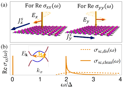
Figure 1: (a) Schematic experimental setups for the measurements of Re $\sigma_{xx}$ and Re $\sigma_{yy}$. The pink layer and orange arrow represent a superconducting film under a linearly polarized light, where $E_{i}(t)=E_{0}e^{-i\omega t}$ is the corresponding electric field in $i=x,y$ directions. A supercurrent $J^{s}_{i}$, which shifts the Fermi surface by a momentum $Q_{i}/2$ is applied along the same direction $i=x,y$ to break the inversion symmetry. (b) Schematic illustration of the optical absorption spectra expected from a clean superconducting state (solid line) and disorders (dashed line). The solid peak at frequency $\omega=2\Delta$ results from the momentum-preserving transition across the gap, whereas the disorder-driven response results from the indirect transitions (see the inset). The zero-frequency solid peak results from the superfluid weight.

Model — To allow non-vanishing optical absorption $\text{Re}\sigma_{ii}(\omega)$ in the superconducting state, we propose to break the inversion symmetry by applying a supercurrent and achieve current relaxation by tuning the chemical potential $\mu$ to VH filling. The BdG Hamiltonian that describes such a VH-driven superconductor is given by

$$H^{\text{BdG}}_{\textbf{q}}(\textbf{Q})=\begin{pmatrix}\xi_{\textbf{q}+\frac{\textbf{Q}}{2}}&\Delta\\ \Delta^{*}&-\xi_{-\textbf{q}+\frac{\textbf{Q}}{2}}\end{pmatrix},$$ (3)

written in the Nambu basis $\Psi_{\textbf{q}}=(c_{\textbf{q}+\frac{\textbf{Q}}{2}\uparrow},c_{-\textbf{q}+\frac{\textbf{Q}}{2}\downarrow}^{\dagger})^{T}$. Here, the normal-state dispersion $\xi_{\textbf{q}}$ is shifted by $\textbf{Q}/2$ in momentum due to the applied current, and $c^{\dagger}_{\textbf{q}s}$ creates an electron with spin $s=\uparrow,\downarrow$ at momentum q away from the VH point. The normal-state dispersion $\xi_{\textbf{q}}=\epsilon_{\textbf{q}}-\mu$ exhibits one or more cVHS or hVHS when the chemical potential $\mu=0$ (see Eq. 1). We assume the superconducting order parameter $\Delta$ is momentum-independent, which can be determined by self-consistenly solving the gap equation in the presence of an on-site interaction $H^{\text{int}}=U\sum_{\textbf{k}\textbf{k}^{\prime}\textbf{p}\sigma\sigma^{\prime}}c^{\dagger}_{\textbf{k}+\textbf{p}\sigma}c^{\dagger}_{\textbf{k}^{\prime}-\textbf{p}\sigma^{\prime}}c_{\textbf{k}^{\prime}\sigma^{\prime}}c_{\textbf{k}\sigma}$ with $U<0$ (see supplementary material (SM) [81] Sec. I). Since the low-energy dispersions $\xi$ are not isotropically parabolic near the saddle point(s), selection rule (2) is fulfilled for the optical absorption in the superconducting state described by $H^{\text{BdG}}_{\textbf{q}}(\textbf{Q})$ .

Within this formalism, the total current density is given by $\textbf{J}=\frac{1}{V}\sum_{\textbf{q}}\Psi_{\textbf{q}}^{\dagger}{\textbf{j}}_{\textbf{q}}\Psi_{\textbf{q}}$, where $V$ is the volume and the current operator has the form

$$\textbf{j}_{\textbf{q}}={\textbf{v}}_{\textbf{q}}\tau^{0}+\mathbb{M}_{\textbf{q}}^{-1}\cdot\frac{\textbf{Q}}{2}~{}\tau^{3}$$ (4)

up to the lowest order in $|\textbf{Q}|$, and $\tau_{i}$ denotes Nambu-basis Pauli matrices. Importantly, the second term breaks the inversion symmetry so that selection rule (i) is fulfilled. Thus, the resulting absorption amplitude is expected to be proportional to the effective mass $(\mathbb{M}_{\textbf{q}}^{-1})_{ij}=\partial_{q_{i}}\partial_{q_{j}}\xi_{\textbf{q}}$ in the normal state.

Optical conductivity with vertex correction— The dissipative optical conductivity in the superconducting state can be calculated by the standard linear response theory as [82]

$$\text{Re}~{}\sigma_{ii}(\omega)=\text{Im}\frac{P_{ii}(i\omega_{m}\rightarrow\omega+i\eta)}{\omega},$$ (5)

where $P_{ii}(i\omega_{m})$ is the current-current correlator and $\omega_{m}$ is the bosonic Mastubara frequency. Importantly, it was shown that the current relaxation due to lattice effects cannot be correctly captured if $P_{ii}(i\omega_{m})$ is calculated from the BdG Hamiltonian $H^{\text{BdG}}_{\textbf{q}}$ since the Ward identity is violated under the mean-field approximation. To restore the Ward identity, it has been shown that it is sufficient to include the corrections from the pairing interaction in $P_{ii}(i\omega_{m})$ under the random phase approximation (RPA) [84, 85]. Specifically, the current-current correlator under RPA is given by

$$P_{ij}(i\omega_{m})=$$

$$~{}~{}-T\sum_{iq_{n}}\frac{1}{V}\int_{\textbf{q}}\text{Tr}\Big{[}j_{\textbf{q},i}G_{iq_{n}+i\omega_{m},\textbf{q}}\Gamma_{\textbf{q},j}(i\omega_{m})G_{iq_{n},\textbf{q}}\Big{]},\quad$$ (6)

where $T$ is the temperature, $q_{n}$ is the fermionic Mastubara frequency, and $G_{iq_{n},\textbf{q}}=(iq_{n}-H^{\text{BdG}}_{\textbf{q}})^{-1}$ is the Green function obtained from the BdG Hamiltonian. Here, $j_{\textbf{q},i}$ and $\Gamma_{\textbf{q},j}(i\omega_{m})=j_{\textbf{q},j}+\delta\Gamma_{\textbf{q},j}(i\omega_{m})~{}(i=x,y)$ are the bare and dressed current operators, where the latter can be obtained by self-consistently solving the following Bethe–Salpeter equation,

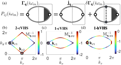
Figure 2: (a) Diagrammatic representations for the total current-current correlator in Eq. 6. The open circle, filled circle, double line, dotted line, and shaded region represent the current vertex, interaction vertex, dressed Green function, density-density interaction, and dressed current operator in Eq. 7, respectively. (b)-(d) The inverse effective mass $\mathbb{M}_{\textbf{q},yy}^{-1}$ along the Fermi surface for the lattice models used to calculate Fig. 3 (a)-(c). These three models show (b) two cVHS at momenta $\textbf{k}_{c1}$ and $\textbf{k}_{c2}$, (c) a single cVHS at $\textbf{k}_{c1}$, and (d) a single hVHS at $\textbf{k}_{c1}$ on the Fermi surface.

$$\bm{\Gamma}_{\textbf{q}}(i\omega_{m})=\textbf{j}_{\textbf{q}}$$

$$~{}~{}-T\sum_{iq_{n}}\frac{1}{V}\int_{\textbf{q}^{\prime}}U\tau^{3}G_{iq_{n}+i\omega_{m},\textbf{q}^{\prime}}\bm{\Gamma}_{\textbf{q}^{\prime}}(i\omega_{m})G_{iq_{n},\textbf{q}^{\prime}}\tau^{3},~{}~{}~{}$$ (7)

with $\tau_{i}$ being the Nambu Pauli matrices. The corresponding ladder diagrams for the resulting current-current correlator $P_{ii}(i\omega_{n})$ are shown in Fig. 2. Finally, the resulting optical conductivity obtained from Eqs. 5-7 is given by

$$\text{Re}~{}\sigma_{ii}(\omega)=\sigma^{(0)}_{ii}(\omega)+\delta\sigma_{ii}(\omega)$$

$$~{}~{}=\Theta(\omega-2|\Delta|)\frac{\pi Q_{i}^{2}|\Delta|^{2}}{2\omega^{2}\sqrt{\omega^{2}-4|\Delta|^{2}}}(\mathcal{C}_{ii}^{(0)}+\delta\mathcal{C}_{ii}),~{}~{}$$ (8)

where $\sigma^{(0)}_{ii}$ is the bare optical conductivity and $\delta\sigma_{ii}$ is the correction resulting from the vertex correction $\delta\Gamma_{\textbf{q}}$ to the current (see SM [81] Sec. II).

The frequency dependence of the optical conductivity $\text{Re}~{}\sigma_{ii}(\omega)$ in Eq. 8 describes a peak at $\omega=2|\Delta|$, which results from the transition across the superconducting gap. For all the numerical calculations in this work, we regulate the peak by assuming a fixed finite scattering rate $\Gamma>0$ [86] so that $\frac{1}{\sqrt{(\omega/2)^{2}-|\Delta|^{2}}}\rightarrow\frac{1}{\sqrt{|\Delta|\Gamma}}$. This is generally expected from reasons such as disorders. The intensity of this peak is determined by the order parameter $\Delta$, the current momentum $Q_{i}$, as well as the normal state properties captured in the intensity factors $\mathcal{C}^{(0)}_{ii}$ and $\delta\mathcal{C}_{ii}$. Specifically, these factors are determined by the effective mass $\mathbb{M}_{\textbf{q},ii}$ and the DOS as

$$\mathcal{C}_{ii}^{(0)}=\int_{\textbf{q}}\delta(\xi_{\textbf{q}})(\mathbb{M}_{\textbf{q},ii}^{-1})^{2},\;\;\delta\mathcal{C}_{ii}=-\frac{\Big{(}\int_{\textbf{q}}\delta(\xi_{\textbf{q}})\mathbb{M}_{\textbf{q},ii}^{-1}\Big{)}^{2}}{\int_{\textbf{q}}\delta(\xi_{\textbf{q}})},\;\;\quad$$ (9)

where $\mathcal{C}^{(0)}_{ii}$ and $\delta\mathcal{C}_{ii}$ originate from the bare current operator $\textbf{j}_{\textbf{q}}$ and the vertex correction $\delta\bm{\Gamma}_{\textbf{q}}(iq_{n})$ in Eq. 7, respectively (see SM [81] Sec. II).

Note that it is clear from Eq. 8 and 9 how selection rules (i) and (ii) forbid the optical absorption. For selection rule (i), Re $\sigma_{ii}(\omega)=0$ when the inversion symmetry is restored by removing the applied current, i.e. $Q_{i}=0$. For selection rule (ii), the current is conserved when the effective mass $\mathbb{M}_{\textbf{q},ii}$ is momentum q-independent. In this case, Eq. 9 indicates that the intensity factors perfectly cancel each other $\mathcal{C}_{ii}^{(0)}+\delta\mathcal{C}_{ii}=0$ so that Re $\sigma_{ii}(\omega)=0$. Since both intensity factors carry divergence from the VHS density of states, when selection rule (ii) is violated, the net intensity $\mathcal{C}_{ii}^{(0)}+\delta\mathcal{C}_{ii}$ can be diverging or non-diverging depending on the cause and degree of current relaxation. In the following, we examine how the net intensity and its anisotropy between $i=x,y$ depend on the number and type of VHS near the Fermi surface.

Superconductivity driven by cVHS— First, we investigate the optical absorption Re $\sigma(\omega)$ in a superconducting state where the Fermi surface contains multiple or one cVHS. Multiple cVHS can naturally occur in the presence of crystalline symmetries, such as discrete rotational symmetries $\mathcal{R}_{n}$, where there are $n_{\text{VH}}=n/2$ and $n$ cVHS located at momenta M, $\mathcal{R}_{n}\textbf{M},\cdots$, for even and odd $n$, respectively, at $\xi_{\textbf{q}}=0$. The case of a single cVHS can then be achieved by breaking the $\mathcal{R}_{n}$ symmetry with external perturbations. For instance, there are typically two $\mathcal{R}_{4}$-related VH points $\textbf{k}=(\pi,0)$ and $(0,\pi)$ on a square lattice. Under an uniaxial strain that breaks the $\mathcal{R}_{4}$ into a $\mathcal{R}_{2}$ symmetry, generally only one of the cVHS survives on the Fermi surface.

For both $n_{\text{VH}}>1$ and $n_{\text{VH}}=1$ cVHS cases, the bare intensity $\mathcal{C}_{ii}^{(0)}$ of the absorption peak at $\omega=2\Delta$ (see Eq. 8) has the general form

$$\mathcal{C}_{\text{cVHS},xx}^{(0)}=a^{(0)}_{xx}\log(\frac{\Lambda_{x}}{\sqrt{\mu/(2\alpha_{1})}})+f_{xx}^{(0)},$$

$$\mathcal{C}_{\text{cVHS},yy}^{(0)}=a^{(0)}_{yy}\log(\frac{\Lambda_{y}}{\sqrt{\mu/(2\beta_{1})}})+f_{yy}^{(0)},\;\;\quad$$ (10)

which contains a log-divergent term resulting from the DOS of cVHS. The coefficients $a^{(0)}_{xx(yy)}$ and the non-divergent terms $f_{xx(yy)}^{(0)}$ depend on the patch widths $\Lambda_{x(y)}$ and dispersion coefficients $\alpha_{1,2}(\beta_{1,2})$ in Eq. 1. See SM Sec. III [81] for the explicit forms in orthorhombic $n=2,4$ and hexagonal $n=3$ systems.

The vertex correction $\delta\mathcal{C}_{ii}$, on the other hand, is sensitive to the number $n_{\text{VH}}$ of cVHS.

• Multiple cVHS $n_{\text{VH}}>1$

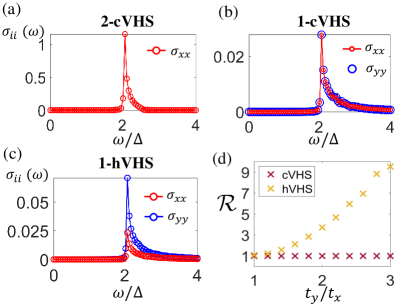
Figure 3: Optical conductivity numerically calculated for clean superconducting lattice models (defined in the text) with different VH patterns on the Fermi surface: (a) two cVHS, (b) single cVHS, (c) single hVHS. All energy scales are expressed in unit of hopping parameters $t=t_{x}=1$. The rest of the hopping parameters are set to be $t_{y}=2,t_{yy}=0$ in (b), and $t_{y}=2,t_{yy}=0.5$ in (c). The sizes of superconducting gap and supercurrent momentum are $|\Delta|=0.1$, $|\textbf{Q}|=0.02$ respectively. (d) The ratio $\mathcal{R}\equiv\text{Re}~{}\sigma_{yy}/\text{Re}~{}\sigma_{xx}$ as a function of $t_{y}/t_{x}$ for the single cVHS and hVHS.

When there are $n_{\text{VH}}>1$ cVHS near the Fermi level, we calculate Eq. 9 and find the vertex corrections to be

$$\delta\mathcal{C}_{\text{cVHS},xx} = \delta a_{xx}\log(\frac{\Lambda_{x}}{\sqrt{\mu/(2\alpha_{1})}})+\delta f_{xx},$$

$$\delta\mathcal{C}_{\text{cVHS},yy} = \delta a_{yy}\log(\frac{\Lambda_{y}}{\sqrt{\mu/(2\beta_{1})}})+\delta f_{yy},,$$ (11)

where $\delta a_{xx(yy)}<0$ and $\delta f_{xx(yy)}<0$ are also analytic functions of $\Lambda_{x(y)}$ and $\alpha_{1(2)},\beta_{1(2)}$. Similar to the bare contributions $\mathcal{C}^{(0)}_{\text{cVHS},ii}$, the vertex corrections $\delta\mathcal{C}_{\text{cVHS},ii}$ contain a log divergent part that comes from the density of states and a non-divergent part that depends on the cVHS dispersions. Importantly, the log divergent terms in $\mathcal{C}^{(0)}_{\text{cVHS},ii}$ and $\delta\mathcal{C}_{\text{cVHS},ii}$ never perfectly cancel, i.e. $a_{xx(yy)}+\delta a_{xx(yy)}>0$ regardless of the dispersion details. Therefore, the net peak intensity in the presence of multiple cVHS is always log divergent $\mathcal{C}^{(0)}_{\text{cVHS},ii}+\delta\mathcal{C}_{\text{cVHS},ii}\propto\log(\frac{\Lambda_{i}}{\sqrt{|\mu|}})$.

The coefficient of this log divergence further depends on the isotropy of specific VHS dispersions in Eq. 2. In the isotropic limit where $\alpha_{1}=\beta_{1}$, the vertex corrections in Eq. 11 vanish $\delta\mathcal{C}_{\text{cVHS},ii}=0$. Thus, the net peak intensity is simply given by the bare intensity $\mathcal{C}^{(0)}_{\text{cVHS},ii}$ so that the full magnitude of log divergence is kept. For anisotropic dispersions with $\alpha_{1}\neq\beta_{1}$, the non-zero vertex corrections $\delta\mathcal{C}_{\text{cVHS},ii}$ partially cancels the bare intensity in Eq. 10 such that the coefficient of the logarithmic divergence decreases.

Table 1: Optical absorption signatures in $s$-wave superconducting states driven by different numbers and types of VHS on the Fermi surface. In each case, the normal state DOS exhibits a characteristic behaviour of divergence. The absorption intensity and the anisotropy ratio $\mathcal{R}\equiv\text{Re}~{}\sigma_{yy}/\text{Re}~{}\sigma_{xx}$ are summarized.

	DOS	Re $\sigma_{ii}(\omega)$	Anisotropy
Multiple cVHS	Log-divergent	Log-divergent	$\mathcal{R}=1$
Single cVHS	Log-divergent	Non-divergent	$\mathcal{R}\approx 1$
Single hVHS	Power-law divergent	Non-divergent	$\mathcal{R}\gg 1$

In Fig. 3 a, we numerically demonstrate the optical absorption spectrum calculated from Eq. 8 on a square lattice with a dispersion $\xi_{\textbf{k}}=-t\cos(k_{x})-t\cos(k_{y})-\mu$. The Van Hove filling is at a chemical potential of $\mu=0$, where there are two cVHS on the Fermi surface at $\textbf{k}_{c1}=(0,\pi)$ and $\textbf{k}_{c2}=(\pi,0)$. Since the dispersions expanded around the two VH points are isotropic, i.e. $\alpha_{1}=\beta_{1}=t$, we numerically find that the net peak intensity fully exhibits the log-divergent peak in the bare intensity, as expected analytically from Eqs. 10 and 11.

• Single cVHS $n_{\text{VH}}=1$

In sharp contrast to the $n_{\text{VH}}>1$ case, we find that the vertex corrections $\delta\mathcal{C}_{\text{cVHS},ii}$ in the single cVHS case perfectly cancel the log divergent term in the bare intensity $\mathcal{C}^{(0)}_{\text{cVHS},ii}$ in Eq. 10, i.e. $a_{xx(yy)}^{(0)}+\delta a_{xx(yy)}=0$. Therefore, regardless of specific VHS dispersions, the net peak intensities are not divergent. Instead, we find that the magnitudes of these non-diverging peak intensities quantitatively depend on dispersion details as

$$\mathcal{C}_{\text{cVHS},xx}^{(0)}+\delta\mathcal{C}_{\text{cVHS},xx}\approx\frac{1}{\Lambda_{x}\Lambda_{y}}\frac{\alpha_{2}^{2}}{\sqrt{\alpha_{1}\beta_{1}}}\frac{\Lambda_{x}^{4}}{4},$$

$$\mathcal{C}_{\text{cVHS},yy}^{(0)}+\delta\mathcal{C}_{\text{cVHS},yy}\approx\frac{1}{\Lambda_{x}\Lambda_{y}}\frac{\beta_{2}^{2}}{\sqrt{\alpha_{1}\beta_{1}}}\frac{\Lambda_{y}^{4}}{4}.\;\;$$ (12)

For purely quadratic cVHS dispersions with $\alpha_{2}=\beta_{2}=0$ (see Eq. 1), the $\omega=2\Delta$ absorption peak completely vanishes since the net intensities in Eq. 12 are zero. The vanishing peak is a consequence of current conservation due to the momentum-independent effective masses. For band structures where the quartic terms naturally exist $\alpha_{2},\beta_{2}\neq 0$, we find non-diverging intensities that quantitatively depend on $\alpha_{2}$ and $\beta_{2}$ (see Eq. 12).

In Fig. 3b, we numerically demonstrate this weak peak considering a rectangular lattice with a single band $\xi_{\textbf{k}}=-t_{x}\cos(k_{x})-t_{y}\cos(k_{y})-t_{yy}\cos(2k_{y})-\mu$. The four-fold rotational symmetry is broken by the difference between the nearest-neighbor hoppings $t_{x}\neq t_{y}$ and next-nearest neighbor hopping $t_{yy}\neq 0$. The Van Hove filling is at $\mu=0$, where a single cVHS at $\textbf{k}_{c1}$ occurs on the Fermi surface. By expanding around $\textbf{k}_{c1}$, we can express the cVHS dispersion coefficients in Eq. 1 in terms of the hopping integrals as $\alpha_{1}=t_{x}$, $\beta_{1}=t_{y}-4t_{yy}$, $\alpha_{2}=-t_{x}/2$, and $\beta_{2}=(-t_{y}+16t_{yy})/2$.

Since there is only one cVHS on the Fermi surface and the dispersion near the VH point is not purely quadratic $\alpha_{2}$, $\beta_{2}\neq 0$, we analytically expect a non-diverging absorption peak at $\omega=2\Delta$ from Eq. 12. In the numerically obtained spectrum in In Fig. 3b, we indeed find a weak peak, where the peak intensity is two orders of magnitudes smaller than the divergent peak in the $n_{\text{VH}}=2$ cVHS case (see Fig. 3a).

Superconductivity driven by hVHS — We consider a hVHS that is quadratic in $q_{x}$ but quartic along $q_{y}$, where the VHS dispersion in Eq. 1 has $\beta_{1}=0$. By calculating the bare and net peak intensities along the $i=x$ direction from Eq. 9, we find

$$\mathcal{C}_{\text{hVHS},xx}^{(0)}\approx\frac{1}{\Lambda_{x}\Lambda_{y}}\frac{\alpha_{1}^{\frac{3}{2}}\Gamma(\frac{1}{4})^{2}}{4\sqrt{2\pi}(\frac{\beta_{2}}{3})^{\frac{1}{4}}}\begin{cases}\frac{\sqrt{2}}{\mu^{\frac{1}{4}}}&\text{for}\;\;\mu>0\\ \frac{1}{|\mu^{\frac{1}{4}}|}&\text{for}\;\;\mu<0\end{cases},$$

$$\mathcal{C}_{\text{hVHS},xx}^{(0)}+\delta\mathcal{C}_{\text{hVHS},xx}\approx\frac{1}{\Lambda_{x}\Lambda_{y}}\frac{\alpha_{2}^{2}}{7\alpha_{1}^{\frac{3}{4}}(\frac{\beta_{2}}{6})^{\frac{1}{4}}}\Lambda_{x}^{\frac{7}{2}},$$ (13)

where $\Gamma(x)$ is the gamma function. Here, the power-law divergence at $\mu\rightarrow 0$ in the bare intensity $\mathcal{C}_{\text{hVHS},xx}^{(0)}$ comes from the divergent DOS and the nearly momentum q-independent effective mass $\mathbb{M}_{\textbf{q},xx}$ (see Eq. 9). Nonetheless, similar to the single cVHS case in Eq. 12, this divergence is perfectly canceled by the vertex correction $\delta\mathcal{C}_{\text{hVHS},xx}$ so that the net intensity is not divergent. The net intensity in the $i=y$ direction is not divergent either. Specifically, we find from Eq. 9 that

$$\mathcal{C}_{\text{hVHS},yy}^{(0)}+\delta\mathcal{C}_{\text{hVHS},yy}\approx\frac{1}{\Lambda_{x}\Lambda_{y}}\frac{\beta_{2}^{2}}{3(\frac{\alpha_{1}\beta_{2}}{6})^{\frac{1}{2}}}\Lambda_{y}^{3}+O(|\frac{\mu}{\beta_{2}}|^{\frac{1}{4}}).\;\;\;\;\;\;$$ (14)

Different from the $i=x$ case, the lack of divergence here is due to the momentum-dependent inverse effective mass $\mathbb{M}^{-1}_{\textbf{q},yy}\sim q_{y}^{2}$ along the direction with quartic dispersion (see Eq. 9 and SM [81] Sec. III).

In Fig. 3c, we numerically demonstrate the analytically predicted non-diverging absorption peak in Eqs. 13 and 14 using a lattice model with a single normal band $\xi_{\textbf{k}}=-t_{x}\cos(k_{x})-t_{y}\cos(k_{y})-t_{y}\cos(2k_{y})/4-\mu$. This dispersion exhibits a hVHS with $\beta_{1}=0$ at $\textbf{k}_{c2}$, where the leading order is quartic in $k_{y}$ but quadratic in $k_{x}$. Consistent with our analytic results, we find that the peak intensities in both $i=x$ and $y$ directions, although not vanishing, are orders of mangitude smaller than the $n=2$ cVHS case with a diverging peak.

Dinstinguish single cVHS and hVHS cases— We summarize our results for different VHS fermiology in Table 1. In short, we expect a diverging absorption peak in Re $\sigma_{ii}(\omega)$ for the multiple cVHS case, but a non-divergent or vanishing peak in cases with a single cVHS or hVHS. For single VHS cases with non-vanishing but order-of-magnitudes weaker peaks, we propose to distinguish whether the normal state contains a cVHS or hVHS qualitatively from the anisotropy between $i=x$ and $y$ (see Fig. 1a). Specifically, the single cVHS case exhibits isotropic intensities $\mathcal{C}_{\text{cVHS},xx}\sim\mathcal{C}_{\text{cVHS},yy}$ regardless of the anisotropy in hopping parameters. However, in the hVHS case, the peak anisotropy sensitively reflects the anisotropy in the hopping parameters. This sharp contrast is clearly shown in Figs. 3b and c.

We quantify this qualitative difference by defining

$$\mathcal{R}\equiv\text{Re}~{}\sigma_{yy}(\omega)/\text{Re}~{}\sigma_{xx}(\omega),$$ (15)

where we show $\mathcal{R}$ for the single cVHS and hVHS cases in Fig. 3d as a function of hopping anisotropy $t_{y}/t_{x}$. For the single cVHS case, we find $\mathcal{R}\sim 1$ regardless of the hopping anisotropy the presence of the anisotropy in dispersion parameters (see Eq. 1). This is because $\Lambda_{y}^{2}/\Lambda_{x}^{2}\approx\alpha_{1}/\beta_{1}$ and $\mathcal{R}\sim\frac{(\beta_{2}/\beta_{1})^{2}}{(\alpha_{2}/\alpha_{1})^{2}}$ so that the dispersion anisotropy is smeared out by the ratios between quadratic and quartic coefficients $\alpha_{1}$ and $\alpha_{2}$ ($\beta_{1}$ and $\beta_{2}$) in the same direction. In contrast, the ratio $\mathcal{R}$ in the hVHS case is sensitive to the dispersion anisotropy. The explicit expression of $\mathcal{R}$ in terms of the dispersion coefficients is shown in SM [81] Sec. III. This is intuitively because the quadratic coefficient $\beta_{1}=0$ vanishes so that the dispersion anisotropy is not smeared out as in the cVHS case.

Discussion — Possible candidate superconductors for experimental verification of our theory include Sr₂RuO₄ films under biaxial strain [87, 88] and uniaxial strain, as well as kagome superconductors $\text{AV}_{3}\text{Sb}_{5}$ (A=K, Rb, Cs) and few-layer graphene-base superconducting systems. Moreover, the presence of disorders can result in a featureless background of spectral weight at a higher frequency range $\omega\leq 2\Delta$ due to indirect optical transitions (see Fig. 1a,b and SM [81] Sec. IV). Therefore, we expect that the non-diverging weak peaks in the single cVHS and hVHS cares are likely to be buried in the disorder-induced background. In contrast, the diverging $2\Delta$ peak in the multiple cVHS cases can survive the disorders.

Acknowledgements — Y.-T.H. acknowledges support from NSF Grant No. DMR-2238748. Y.-T.H. acknowledges support from Department of Energy Basic Energy Science Award DE-SC0024291. H.-J.Y. is supported by the Society of Science Fellows Postdoctoral Program in the College of Science.

These Supplementary Materials contain the details on I. Galilean invariance, II. Optical conductivity calculations, III. Peak intensity and IV. Effect of disorder.

I Galilean invariance

In this section, we summarize how the Galilean invariance is related to the absence of optical absorption in superconductors.

I.1 Galilean transformation

Here, we show that the system is Galilean-invariant if the effective mass is a constant tensor. This is the case of $\alpha_{2}=\beta_{2}=0$ which results in $\text{Re}\sigma_{ij}(\omega)=0$ in the main text.

We assume that the kinetic $\hat{T}$ and interaction $\hat{V}$ terms in $\hat{H}[\hat{\textbf{x}}_{\alpha},\hat{\textbf{p}}_{\alpha}]=\hat{T}+\hat{V}$ depend on the momentum and position operators only, i.e. $\hat{T}\equiv\hat{T}[\hat{\textbf{p}}_{\alpha}]$ and $\hat{V}\equiv\hat{V}[\hat{\textbf{x}}_{\alpha}]$, respectively. The Galilean transformation relates two reference frames separated by a constant velocity v,

$$\hat{U}_{\mathcal{G}}(t)^{-1}\hat{\textbf{x}}_{\alpha}\hat{U}_{\mathcal{G}}(t)=\hat{\textbf{x}}_{\alpha}+\textbf{v}t,\qquad\hat{U}_{\mathcal{G}}(t)^{-1}\hat{\textbf{p}}_{\alpha}\hat{U}_{\mathcal{G}}(t)=\hat{\textbf{p}}_{\alpha}+\textbf{m}_{\alpha}\cdot\textbf{v},$$ (S1)

which can be realized by the unitary transformation (within the first quantization) [89],

$$\hat{U}_{\mathcal{G}}(t)=e^{-i\textbf{v}\cdot\sum_{\alpha}(\hat{\textbf{p}}_{\alpha}t-\textbf{m}_{\alpha}\cdot\hat{\textbf{x}}_{\alpha})},$$ (S2)

where $\hat{\textbf{x}}_{\alpha}$ and $\hat{\textbf{p}}_{\alpha}$ are position and momentum operators of particle $\alpha$ which are canonically conjugate each other, $[\hat{x}_{\alpha,i},\hat{p}_{\beta,j}]=i\delta_{\alpha\beta}\delta_{ij}$. Also, the inverse of mass tensor $(\textbf{m}_{\alpha})^{-1}$ is defined by the quadratic coefficients in the kinetic term,

$$\hat{T}=\frac{1}{2}\sum_{\alpha}\sum_{ij}(m_{\alpha})^{-1}|_{ij}\hat{p}_{\alpha,i}\hat{p}_{\alpha,j}+...,$$ (S3)

where $...$ includes higher-order terms in $\hat{p}_{\alpha,i}$. For an arbitrary wavefunction $|\psi(t)\rangle$ satisfying the Schrödinger equation, $\Big{(}i\partial_{t}-\hat{H}\Big{)}|\psi(t)\rangle=0$, the transformed wavefunction $|\psi^{\prime}(t)\rangle=\hat{U}_{\mathcal{G}}(t)|\psi(t)\rangle$ should also satisfy $\Big{(}i\partial_{t}-\hat{H}\Big{)}|\psi^{\prime}(t)\rangle=0$ if the Hamiltonian $\hat{H}$ is invariant under Eq. S2. This results in

$$\hat{U}^{-1}_{\mathcal{G}}\hat{H}\hat{U}_{\mathcal{G}}=\hat{H}+i\hat{U}^{-1}_{\mathcal{G}}\partial_{t}\hat{U}_{\mathcal{G}}.$$ (S4)

Since $\hat{V}[\hat{\textbf{x}}_{\alpha}]$ depends on $\hat{\textbf{x}}_{\alpha}$ only, $\hat{V}[\hat{\textbf{x}}_{\alpha}]$ is invariant under Eq. S1 if $\hat{V}[\hat{\textbf{x}}_{\alpha}]$ is translational-invariant, i.e. $\hat{U}_{\mathcal{G}}^{-1}\hat{V}\hat{U}_{\mathcal{G}}=\hat{V}$. Using Eq. S2,

$$i\hat{U}_{\mathcal{G}}^{-1}\partial_{t}\hat{U}_{\mathcal{G}}=\hat{U}_{\mathcal{G}}^{-1}(\textbf{v}\cdot\hat{\textbf{P}}-\frac{1}{2}\textbf{v}\cdot\textbf{M}\cdot\textbf{v})\hat{U}_{\mathcal{G}}=\textbf{v}\cdot\hat{\textbf{P}}+\frac{1}{2}\textbf{v}\cdot\textbf{M}\cdot\textbf{v},$$ (S5)

where $\textbf{M}=\sum_{\alpha}\textbf{m}_{\alpha}$ and $\hat{\textbf{P}}=\sum_{\alpha}\hat{\textbf{p}}_{\alpha}$. Also,

$$\hat{U}_{\mathcal{G}}^{-1}\hat{T}\hat{U}_{\mathcal{G}} = \frac{1}{2}\sum_{\alpha}(\hat{\textbf{p}}_{\alpha}+\textbf{m}_{\alpha}\cdot\textbf{v})\cdot\textbf{m}^{-1}_{\alpha}\cdot(\hat{\textbf{p}}_{\alpha}+\textbf{m}_{\alpha}\cdot\textbf{v})+...$$ (S6)

$$= \frac{1}{2}\sum_{\alpha}(\hat{\textbf{p}}_{\alpha}\cdot\textbf{m}^{-1}_{\alpha}\cdot\hat{\textbf{p}}_{\alpha})+\textbf{v}\cdot\hat{\textbf{P}}+\frac{1}{2}\textbf{v}\cdot\textbf{M}\cdot\textbf{v}+...,$$

where $...$ includes higher-order terms likewise Eq. S3. Thus the invariance, Eq. S4 holds in the absence of higher terms in Eq. S3, i.e. when $\hat{T}[\hat{\textbf{p}}_{\alpha}]=\frac{1}{2}\sum_{\alpha}\hat{\textbf{p}}_{\alpha}\cdot\textbf{m}^{-1}_{\alpha}\cdot\hat{\textbf{p}}_{\alpha}$.

I.2 Current conservation

The selection rule (2) in the main text indicates that the $\omega=2|\Delta|$ peak in optical absorption can only exist when the current is not conserved. This condition can be understood as follows. In a translational invariant system, the current change rate can be written as

$$\frac{d\textbf{J}(\tau)}{d\tau}=[H^{\text{int}},\textbf{J}(\tau)]=\frac{U}{2V}\sum_{\textbf{k}\textbf{k}^{\prime}\textbf{p}\sigma\sigma^{\prime}}c^{\dagger}_{\textbf{k}+\textbf{p}\sigma}c^{\dagger}_{\textbf{k}^{\prime}-\textbf{p}\sigma^{\prime}}c_{\textbf{k}^{\prime}\sigma^{\prime}}c_{\textbf{k}\sigma}(\Delta\textbf{v}_{\textbf{k}\textbf{k}^{\prime},\textbf{p}}),\;\;$$ (S7)

where $\textbf{J}(\tau)=e^{\tau H}\textbf{J}e^{-\tau H}$, $\textbf{J}=\frac{1}{V}\sum_{\textbf{k}\sigma}\textbf{v}_{\textbf{k}}c_{\textbf{k}\sigma}^{\dagger}c_{\textbf{k}\sigma}$ is the total current density and the change in velocity during a collision is given by $\Delta\textbf{v}_{\textbf{k}\textbf{k}^{\prime},\textbf{p}}=\textbf{v}_{\textbf{k}+\textbf{p}}+\textbf{v}_{\textbf{k}^{\prime}-\textbf{p}}-\textbf{v}_{\textbf{k}^{\prime}}-\textbf{v}_{\textbf{k}}$. Due to momentum conservation, the change in velocity $\Delta\textbf{v}_{\textbf{k}\textbf{k}^{\prime},\textbf{p}}$ vanishes for all momenta $\textbf{k},\textbf{k}^{\prime},\textbf{p}$ when the velocity is proportional to the momentum $\textbf{v}_{\textbf{k}}\propto\textbf{k}$. In such a current-conserving (i.e. Galilean symmetric) system, the current-current correlator,

$$P_{ij}(i\omega_{m})=-\frac{1}{V}\int_{0}^{\beta}d\tau e^{i\omega_{m}\tau}\langle J_{i}(\tau)J_{j}(0)\rangle$$ (S8)

vanishes with the vanishing current change rate $\frac{d\textbf{J}}{d\tau}$ since

$$P_{ij}(i\omega_{m})=\frac{1}{V}\frac{1}{(i\omega_{m})^{2}}\int_{0}^{\beta}d\tau e^{i\omega_{m}\tau}\langle\frac{dJ_{i}(\tau)}{d\tau}\frac{dJ_{j}(0)}{d\tau}\rangle$$ (S9)

by performing integration by part twice. Therefore, the optical absorption vanishes Re$\sigma_{ii}(\omega)=0$ in current-conserving systems. The most common example occurs when the normal state has a parabolic dispersion $\epsilon_{\textbf{k}}=|\textbf{k}|^{2}/(2m)-\mu$, where k, $m$, and $\mu$ are the momentum, electron mass, and chemical potential, respectively. The velocity operator in this case is given by $\textbf{v}_{\textbf{k}}=\textbf{k}/m\propto\textbf{k}$ [89] so that the optical absorption Re$\sigma_{ii}(\omega)=0$ [80]. More generally speaking, the current is nearly conserved in systems with an effective mass $\mathbb{M}_{\textbf{q}}$ that is nearly momentum independent. Note that even in crystals with non-parabolic band structures, this condition is still commonly satisfied when the superconducting gap develops not too far from the band bottom so that the normal band is still nearly parabolic.

II Optical conductivity calculations

This section include the calculation details for the optical absorptions in $s$-wave superconductors. Starting from the BdG (Bogoliubov-de Gennes) Hamiltonian and its vertex correction, then we apply them to the VHS dispersions.

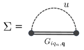
Figure S1: Diagrammatic representation of Eq. S13 whose off-diagonal correction reads the gap equation. The expansion of $\Sigma$ in terms of the bare Green function includes only no-line-crossing diagrams likewise Fig. 2.

II.1 BdG Hamiltonian

In the main text, we consider the BdG Hamiltonian when the normal state Fermi surface is entirely shifted by $\textbf{Q}/2$,

$${H}^{\text{BdG}}_{\textbf{q}}=\begin{pmatrix}\xi_{\textbf{q}+\frac{\textbf{Q}}{2}}&\Delta\\ \Delta&-\xi_{-\textbf{q}+\frac{\textbf{Q}}{2}}\end{pmatrix}=\delta\xi_{\textbf{q}}\tau^{0}+\bar{\xi}_{\textbf{q}}\tau^{3}+\Delta\tau^{1}.$$ (S10)

on the basis ${\Psi}_{\textbf{q}}=\begin{pmatrix}c_{\textbf{q}+\textbf{Q}/2,\uparrow}\\ c_{-\textbf{q}+\textbf{Q}/2,\downarrow}^{\dagger}\end{pmatrix}$ and the BdG Green function in frequency space is

$$G_{iq_{n},\textbf{q}}=(iq_{n}\tau^{0}-H_{\textbf{q}}^{\text{BdG}})^{-1}=\frac{1}{(iq_{n}-\delta\xi_{\textbf{q}})^{2}-E_{\textbf{q}}^{2}}\Big{[}(iq_{n}-\delta\xi_{\textbf{q}})\tau^{0}+\bar{\xi}_{\textbf{q}}\tau^{3}+\Delta\tau^{1}\Big{]},$$ (S11)

where $\omega_{n}$ is the fermionic Matsubara frequency and $\bar{\xi}_{\textbf{q}}=\frac{\xi_{\textbf{q}+\textbf{Q}/2}+\xi_{-\textbf{q}-\textbf{Q}/2}}{2}$, $\delta{\xi}_{\textbf{q}}=\frac{\xi_{\textbf{q}+\textbf{Q}/2}-\xi_{-\textbf{q}-\textbf{Q}/2}}{2}$.

The $s$-wave superconducting order parameter $\Delta$ (fixed to be real) is self-consistently determined by the gap equation at $T=0$,

$$\Delta=-u\int_{\textbf{q}}\frac{\Delta}{2\sqrt{\bar{\xi}_{\textbf{q}}^{2}+|\Delta|^{2}}},$$ (S12)

which is obtained by decoupling the full Hamiltonian, $H^{\text{full}}=\sum_{\textbf{k}\sigma}\xi_{\textbf{k}}c^{\dagger}_{\textbf{k}\sigma}c_{\textbf{k}\sigma}+\frac{1}{2V}\sum_{\textbf{k}\textbf{k}^{\prime}\textbf{p}\sigma\sigma^{\prime}}u~{}(c^{\dagger}_{\textbf{k}+\textbf{p}\sigma}c^{\dagger}_{\textbf{k}^{\prime}-\textbf{p}\sigma^{\prime}}c_{\textbf{k}^{\prime}\sigma^{\prime}}c_{\textbf{k}\sigma})$ with $u<0$. In Eq. S12, we denote $\int_{\textbf{q}}=\frac{1}{V}\sum_{\textbf{q}}$ for notational simplicity. In the self-energy (Fig. S1), the diagonal correction is ignored, and Eq. S12 is the off-diagonal correction of [84, 85]

$$\Sigma=T\sum_{iq_{n}}\int_{\textbf{q}}u~{}\tau^{3}G_{iq_{n},\textbf{q}}\tau^{3},$$ (S13)

which follows the same approximation scheme in the current-current correlation calculation (Fig. 2 in the main text).

For small $|\textbf{Q}|$, we have $\bar{\xi}_{\textbf{q}}=\xi_{\textbf{q}}+O(|\textbf{Q}|^{2})$ and $\delta{\xi}_{\textbf{q}}=\frac{1}{2}\textbf{v}_{\textbf{q}}\cdot\textbf{Q}+O(|\textbf{Q}|^{2})$ with $\textbf{v}_{\textbf{q}}=\nabla_{\textbf{q}}\xi_{\textbf{q}}$. Then, the eigenvalues of Eq. S10 are given by,

$$\tilde{E}_{\textbf{q}}^{\pm}=\pm E_{\textbf{q}}+\frac{1}{2}\textbf{v}_{\textbf{q}}\cdot\textbf{Q},$$ (S14)

where $E_{\textbf{q}}=\sqrt{\xi_{\textbf{q}}^{2}+|\Delta|^{2}}$ is the Bogoliubov dispersion in the absence of applied supercurrent Q. The magnitude of Q is assumed to be small enough so that the spectrum Eq. S14 is gapped for all q.

II.2 Vertex correction

The total current and bare current operator are $\textbf{j}=\sum_{\textbf{q}}\Psi^{\dagger}_{\textbf{q}}\textbf{j}_{\textbf{q}}\Psi_{\textbf{q}}$ and $\textbf{j}_{\textbf{q}}=-e\textbf{v}_{\textbf{q}}^{\text{BdG}}$ ($e>0$) respectively where $\textbf{v}_{\textbf{q}}^{\text{BdG}}$ is the velocity operator,

$$\textbf{v}_{\textbf{q}}^{\text{BdG}}=\begin{pmatrix}\textbf{v}_{\textbf{q}+\frac{\textbf{Q}}{2}}&0\\ 0&\textbf{v}_{\textbf{q}-\frac{\textbf{Q}}{2}}\end{pmatrix}=\bar{\textbf{v}}_{\textbf{q}}\tau^{0}+\delta\textbf{v}_{\textbf{q}}\tau^{3}.$$ (S15)

Here, $\bar{\textbf{v}}_{\textbf{q}}=\nabla_{\textbf{q}}\bar{\xi}_{\textbf{q}}=\nabla_{\textbf{q}}\xi_{\textbf{q}}+O(|\textbf{Q}|^{2})$ and $\delta\textbf{v}_{\textbf{q}}=\nabla_{\textbf{q}}\delta\xi_{\textbf{q}}=\frac{1}{2}\mathbb{M}_{\textbf{q}}^{-1}\cdot\textbf{Q}+O(|\textbf{Q}|^{2})$ where $(\mathbb{M}_{\textbf{q}}^{-1})_{ij}=\partial_{q_{i}}\partial_{q_{j}}\xi_{\textbf{q}}$ is the inverse effective mass. To calculate the current-current correlation,

$$P_{ij}(i\omega_{m})=-T\sum_{iq_{n}}\int_{\textbf{q}}\text{Tr}\Big{[}j_{\textbf{q},i}G_{iq_{n}+i\omega_{m},\textbf{q}}\Gamma_{\textbf{q},j}(i\omega_{m})G_{iq_{n},\textbf{q}}\Big{]},\quad$$ (S16)

the dressed current operator,

$$\bm{\Gamma}_{\textbf{q}}(i\omega_{m})=-e\Big{(}\textbf{v}_{\textbf{q}}^{\text{BdG}}+\delta\bm{\Gamma_{\textbf{q}}}(i\omega_{m})\Big{)},$$ (S17)

and the vertex correction $\delta\bm{\Gamma}_{\textbf{q}}(i\omega_{m})\equiv\sum_{i}(\delta\bm{\Gamma}_{\textbf{q}}(i\omega_{m}))_{i}\tau^{i}$ are introduced to satisfy the Ward identity [84],

$$p_{\mu}\tilde{\Gamma}_{\textbf{q}+\textbf{p},\textbf{q}}^{\mu}(iq_{n}+i\omega_{m},iq_{n})=G^{-1}_{iq_{n}+i\omega_{m},\textbf{q}+\textbf{p}}\tau^{3}-\tau^{3}G^{-1}_{iq_{n},\textbf{q}},$$ (S18)

with $\Gamma_{\textbf{q},j}(i\omega_{m})=\tilde{\Gamma}^{j}_{\textbf{q},\textbf{q}}(iq_{n}+i\omega_{m},iq_{n})$. Using Eqs. S11 and S18, we have $\delta\bm{\Gamma}_{\textbf{q}}(i\omega_{m})=(\delta\bm{\Gamma}(i\omega_{m}))_{2}\tau^{2}$ for some function $(\delta\bm{\Gamma}(iq_{m}))_{2}$ [85, 79] since the diagonal correction in Eq. S13 is ignored. Inserting this into the Bethe–Salpeter equation,

$$\bm{\Gamma}_{\textbf{q}}(i\omega_{m})=\textbf{j}_{\textbf{q}}-T\sum_{iq_{n}}\int_{\textbf{q}^{\prime}}u\tau^{3}G_{iq_{n}+i\omega_{m},\textbf{q}^{\prime}}\bm{\Gamma}_{\textbf{q}^{\prime}}(i\omega_{m})G_{iq_{n},\textbf{q}^{\prime}}\tau^{3},~{}~{}~{}$$ (S19)

leads to,

$$(\delta{\bm{\Gamma}}(i\omega_{m}))_{2}=-T\sum_{iq_{n}}\int_{\textbf{q}}u\frac{1}{(iq_{n}+i\omega_{m}-\delta\xi_{\textbf{q}})^{2}-E_{\textbf{q}}^{2}}\frac{1}{(iq_{n}-\delta\xi_{\textbf{q}})^{2}-E_{\textbf{q}}^{2}}$$

$$\qquad\qquad\qquad\times\Big{[}(\delta\bm{\Gamma}(i\omega_{m}))_{2}\Big{(}-(iq_{n}+i\omega_{m}-\delta\xi_{\textbf{q}})(iq_{n}-\delta\xi_{\textbf{q}})+E_{\textbf{q}}^{2}\Big{)}-i(i\omega_{m}\Delta\delta{\textbf{v}}_{\textbf{q}})\Big{]},$$ (S20)

where the q-dependence in $(\delta{\bm{\Gamma}}(i\omega_{m}))_{2}$ vanishes since the the interaction strength $u$ has no q-dependence. The Mastubara sum in Eq. S20 can be done by

$$T\sum_{iq_{n}}\frac{1}{(iq_{n}+i\omega_{m}-\delta\xi_{\textbf{q}})^{2}-E_{\textbf{q}}^{2}}\frac{1}{(iq_{n}-\delta\xi_{\textbf{q}})^{2}-E_{\textbf{q}}^{2}}$$

$$\qquad\qquad\qquad\qquad=\frac{1}{4E_{\textbf{q}}^{2}}\Big{(}n_{F}(\delta\xi_{\textbf{q}}+E_{\textbf{q}})-n_{F}(\delta\xi_{\textbf{q}}-E_{\textbf{q}})\Big{)}\Big{(}\frac{1}{i\omega_{m}-2E_{\textbf{q}}}-\frac{1}{i\omega_{m}+2E_{\textbf{q}}}\Big{)},$$

$$T\sum_{iq_{n}}\frac{iq_{n}+i\omega_{m}-\delta\xi_{\textbf{q}}}{(iq_{n}+i\omega_{m}-\delta\xi_{\textbf{q}})^{2}-E_{\textbf{q}}^{2}}\frac{iq_{n}-\delta\xi_{\textbf{q}}}{(iq_{n}-\delta\xi_{\textbf{q}})^{2}-E_{\textbf{q}}^{2}},$$

$$\qquad\qquad\qquad\qquad=-\frac{1}{4}\Big{(}n_{F}(\delta\xi_{\textbf{q}}+E_{\textbf{q}})-n_{F}(\delta\xi_{\textbf{q}}-E_{\textbf{q}})\Big{)}\Big{(}\frac{1}{i\omega_{m}-2E_{\textbf{q}}}-\frac{1}{i\omega_{m}+2E_{\textbf{q}}}\Big{)},$$ (S21)

where $n_{F}(E)=1/(e^{\beta E}+1)$ ($\beta=1/T$) is the Fermi distribution. At $T=0$, Eq. S20 reads,

$$-u\Big{(}\int_{\textbf{q}}\frac{1}{2E_{\textbf{q}}}+\frac{2E_{\textbf{q}}}{(i\omega_{m})^{2}-4E_{\textbf{q}}^{2}}\Big{)}(\delta{\bm{\Gamma}}(i\omega_{m}))_{2}=-u\int_{\textbf{q}}\frac{1}{E_{\textbf{q}}}\frac{1}{(i\omega_{m})^{2}-4E_{\textbf{q}}^{2}}i(i\omega_{m}\Delta\delta\textbf{v}_{\textbf{q}}),$$ (S22)

using Eq. S12. Then,

$$(\delta{\bm{\Gamma}}(i\omega_{m}))_{2}=\frac{2i\Delta}{i\omega_{m}}\frac{I_{i\omega_{m}}[\delta\textbf{v}_{\textbf{q}}]}{I_{i\omega_{m}}[1]},$$ (S23)

where

$$I_{i\omega_{m}}[f_{\textbf{q}}]=\int_{\textbf{q}}\frac{1}{E_{\textbf{q}}}\frac{f_{\textbf{q}}}{(i\omega_{m})^{2}-4E_{\textbf{q}}^{2}},$$ (S24)

is a functional of $f_{\textbf{q}}$ [85].

II.3 Current-current correlation

Here, we derive Eqs. 8 and 9 in the main text. The bare current-current correlation and its correction are,

$$P^{(0)}_{ij}(i\omega_{m})=-e^{2}T\sum_{iq_{n}}\int_{\textbf{q}}\text{Tr}\Big{[}{v}_{\textbf{q},i}^{\text{BdG}}G_{iq_{n}+i\omega_{m},\textbf{q}}{v}_{\textbf{q},j}^{\text{BdG}}G_{iq_{n},\textbf{q}}\Big{]},$$ (S25)

and

$$\delta P_{ij}(i\omega_{m})=-e^{2}T\sum_{iq_{n}}\int_{\textbf{q}}\text{Tr}\Big{[}{v}_{\textbf{q},i}^{\text{BdG}}G_{iq_{n}+i\omega_{m},\textbf{q}}\delta\Gamma_{\textbf{q},j}(i\omega_{m})G_{iq_{n},\textbf{q}}\Big{]}.$$ (S26)

Inserting Eqs. S11 and S15 into Eq. S25, we have

$$P_{ij}^{(0)}(i\omega_{m})=-4e^{2}\Delta^{2}I_{i\omega_{m}}[\delta v_{\textbf{q},i}\delta v_{\textbf{q},j}]$$ (S27)

using Eq. S21. Similarly, the correction term Eq. S26 becomes

$$\delta P_{ij}(i\omega_{m})=4e^{2}\Delta^{2}\frac{I_{i\omega_{m}}[\delta v_{\textbf{q},i}]I_{i\omega_{m}}[\delta v_{\textbf{q},j}]}{I_{i\omega_{m}}[1]}.$$ (S28)

The numerical calculations (Fig. 3 in the main text) are done by inserting the lattice dispersion into Eqs. S27 and S28. If the effective mass is constant in q-space, $\delta\textbf{v}_{\textbf{q}}$ has also no q-dependence and $P_{ij}^{(0)}+\delta P_{ij}=0$.

With the analytic continuation $i\omega_{m}\rightarrow\omega+i\eta$,

$$\text{Im}I_{\omega+i\eta}[f_{\textbf{q}}] = -\frac{\pi}{\omega^{2}}\int_{\textbf{q}}\delta(\omega-2E_{\textbf{q}})f_{\textbf{q}}=-\frac{\pi}{4\omega\sqrt{(\frac{\omega}{2})^{2}-|\Delta|^{2}}}\Theta(\omega-2|\Delta|)\int_{\textbf{q}}\delta\Big{(}\xi_{\textbf{q}}-\sqrt{(\frac{\omega}{2})^{2}-|\Delta|^{2}}\Big{)}f_{\textbf{q}}$$ (S29)

$$\approx -\frac{\pi}{4\omega\sqrt{(\frac{\omega}{2})^{2}-|\Delta|^{2}}}\Theta(\omega-2|\Delta|)\int_{\textbf{q}}\delta(\xi_{\textbf{q}})f_{\textbf{q}},$$

where the identity $\delta(F(x)-F(x_{0}))=\delta(x-x_{0})|dF/dx|^{-1}_{x=x_{0}}$ is used and the last approximation holds close to the gap edge $\omega\approx 2|\Delta|$. For $\omega\approx 2|\Delta|$, the imaginary part of $I_{\omega+i\eta}$ is much larger than the real part so Eqs. S27 and S28 can be simplified using Eq. S29. Then, the optical absorption $\text{Re}~{}\sigma_{ij}=\sigma_{ij}^{(0)}+\delta\sigma_{ij}$ is

$$\sigma_{ij}^{(0)}(\omega)=\text{Im}\frac{P_{ij}^{(0)}(\omega+i\eta)}{\omega}=\Theta(\omega-2|\Delta|)\frac{e^{2}\pi|\Delta|^{2}}{2\omega^{2}\sqrt{\omega^{2}-4|\Delta|^{2}}}\sum_{i^{\prime}j^{\prime}}\tilde{\mathcal{C}}^{(0)}_{ii^{\prime},jj^{\prime}}Q_{i^{\prime}}Q_{j^{\prime}},$$ (S30)

$$\delta\sigma_{ij}(\omega)=\text{Im}\frac{\delta P_{ij}(\omega+i\eta)}{\omega}=\Theta(\omega-2|\Delta|)\frac{e^{2}\pi|\Delta|^{2}}{2\omega^{2}\sqrt{\omega^{2}-4|\Delta|^{2}}}\sum_{i^{\prime}j^{\prime}}\delta\tilde{\mathcal{C}}_{ii^{\prime},jj^{\prime}}Q_{i^{\prime}}Q_{j^{\prime}},\quad$$ (S31)

where the peak intensities of optical absorption,

$$\tilde{\mathcal{C}}^{(0)}_{ii^{\prime},jj^{\prime}}=\int_{\textbf{q}}\delta(\xi_{\textbf{q}})(\mathbb{M}^{-1}_{\textbf{q},ii^{\prime}})(\mathbb{M}^{-1}_{\textbf{q},jj^{\prime}}),\qquad\delta\tilde{\mathcal{C}}_{ii^{\prime},jj^{\prime}}=-\frac{\int_{\textbf{q}}\delta(\xi_{\textbf{q}})(\mathbb{M}^{-1}_{\textbf{q},ii^{\prime}})\int_{\textbf{q}}\delta(\xi_{\textbf{q}})(\mathbb{M}^{-1}_{\textbf{q},jj^{\prime}})}{\int_{\textbf{q}}\delta(\xi_{\textbf{q}})},$$ (S32)

are determined by the integral of inverse effective mass along the normal state Fermi surface. In the main text, we consider the case of $\mathbb{M}^{-1}_{\textbf{q},xy}=0$ with $\textbf{Q}=Q\hat{x}$ or $\textbf{Q}=Q\hat{y}$, then $\mathcal{C}_{ii}^{(0)}=\tilde{\mathcal{C}}_{ii,ii}^{(0)},\delta{\mathcal{C}}_{ii}=\delta\tilde{\mathcal{C}}_{ii,ii}$ in Eq. 9.

III Peak intensity

Here, Eqs. 10-12 are derived and the expressions of non-diverging parts are shown.

III.1 Multiple cVHS dispersion

When the system preserves the $n$-fold rotational symmetry $\mathcal{R}_{n}$, there are multiple VHS at $\textbf{M},\mathcal{R}_{n}\textbf{M},\mathcal{R}_{n}^{2}\textbf{M},...$ at the Fermi surface. In this case, the sum of effective mass at $\textbf{M},\mathcal{R}_{n}\textbf{M},\mathcal{R}_{n}^{2}\textbf{M},...$ cancels each other and $\int_{\textbf{q}}\delta(\xi_{\textbf{q}})(\mathbb{M}^{-1}_{\textbf{q},ij})$ in the vertex correction Eq. S31 is small compared to the bare intensity. For example, for the square lattice dispersion,

$$\xi_{\textbf{k}}=-t\cos(k_{x})-t\cos(k_{y})-t^{\prime}\cos(2k_{x})-t^{\prime}\cos(2k_{y})-\mu,$$ (S33)

there are two-cVHS at $\textbf{M}_{1}=(0,\pi)$ and $\textbf{M}_{2}=(\pi,0)$ as long as $|t|>4|t^{\prime}|$. Close to $\textbf{M}_{1,2}$, the continuum dispersions are

$$\xi_{\textbf{q}=\textbf{k}-\textbf{M}_{1}}=\frac{\alpha}{2}q_{x}^{2}-\frac{\beta}{2}q_{y}^{2}+O(q_{x}^{4},q_{y}^{4}),\qquad\xi_{\textbf{q}=\textbf{k}-\textbf{M}_{2}}=-\frac{\beta}{2}q_{x}^{2}+\frac{\alpha}{2}q_{y}^{2}+O(q_{x}^{4},q_{y}^{4})$$ (S34)

where $\alpha=t+4t^{\prime},\beta=t-4t^{\prime},\mu=-2t^{\prime}$ and these dispersions are related by $\mathcal{R}_{4}$ rotational symmetry.

When $t^{\prime}=0$, then $\alpha=\beta$ which results in $\int_{\textbf{q}}\delta(\xi_{\textbf{q}})(\mathbb{M}^{-1}_{\textbf{q},ij})=0$ and $\delta\sigma_{ij}=0$. Due to the $\mathcal{R}_{4}$ rotational symmetry, $\sigma_{xx}=\sigma_{yy}$ and its intensity can be calculated using Eq. S33,

$$\mathcal{C}^{(0)}_{xx}=\int_{\textbf{k}}\delta(\xi_{\textbf{k}})(\mathbb{M}^{-1}_{\textbf{k},xx})^{2}=4t\int_{\Lambda_{0}}^{\pi-\Lambda_{0}}\frac{dk_{x}dk_{y}}{(2\pi)^{2}}\delta(k_{x}-k_{y}+\pi)\frac{\cos^{2}k_{x}}{|\sin k_{x}|}\approx\frac{2t}{\pi^{2}}\log\frac{1}{\Lambda_{0}},$$ (S35)

where the diverging integral is regulated by the long wavelength cut-off $\Lambda_{0}=O(1/L)$ with the linear system size $L$. In this case, the log-divergence in Eq. S35 and Eq. S30 are not cancelled by the vertex correction and the peak intensity of $\text{Re}\sigma_{ii}$ is very large (Fig. 3a in the main text).

The log-divergence of bare intensity still survives for $t^{\prime}\neq 0$. Using Eqs. S32 and S34, the bare intensity and vertex correction are

$$\mathcal{C}_{xx}^{(0)} \approx \frac{1}{\pi^{2}}\frac{\alpha^{2}+\beta^{2}}{\sqrt{\alpha\beta}}\log\frac{1}{\Lambda_{0}},\qquad\delta\mathcal{C}_{xx}\approx-\frac{1}{\pi^{2}}\frac{(\alpha-\beta)^{2}}{2\sqrt{\alpha\beta}}\log\frac{1}{\Lambda_{0}}.$$ (S36)

For $\alpha,\beta>0$, the log-divergence is not perfectly cancelled in the net intensity,

$$\mathcal{C}_{xx}^{(0)}+\delta\mathcal{C}_{xx}\approx\frac{1}{\pi^{2}}\frac{(\alpha+\beta)^{2}}{2\sqrt{\alpha\beta}}\log\frac{1}{\Lambda_{0}}.$$ (S37)

Finally, we check the net intensity when the system preserves the 3-fold rotational symmetry, e.g. kagome or honeycomb lattice. We consider $\mathcal{R}_{3}$-related three VH points at $\textbf{M}_{1}=(0,\frac{2\pi}{\sqrt{3}}),\textbf{M}_{2}=(\pi,\frac{\pi}{\sqrt{3}}),\textbf{M}_{3}=(-\pi,\frac{\pi}{\sqrt{3}})$ [39] whose dispersions upto the quadratic orders are

$$\xi_{\textbf{q}=\textbf{k}-\textbf{M}_{1}}=\frac{\alpha}{2}q_{x}^{2}-\frac{\beta}{2}q_{y}^{2},\qquad\quad\xi_{\textbf{q}=\textbf{k}-\textbf{M}_{2}}=\frac{1}{2}(\frac{\alpha}{4}-\frac{3\beta}{4})q_{x}^{2}-(\frac{\sqrt{3}\alpha}{2}+\frac{\sqrt{3}\beta}{2})q_{x}q_{y}+\frac{1}{2}(\frac{3\alpha}{4}-\frac{\beta}{4})q_{y}^{2},$$

$$\xi_{\textbf{q}=\textbf{k}-\textbf{M}_{3}}=\frac{1}{2}(\frac{\alpha}{4}-\frac{3\beta}{4})q_{x}^{2}+(\frac{\sqrt{3}\alpha}{2}+\frac{\sqrt{3}\beta}{2})q_{x}q_{y}+\frac{1}{2}(\frac{3\alpha}{4}-\frac{\beta}{4})q_{y}^{2}.$$ (S38)

The bare intensity and vertex correction for Eq. S38 are

$$\mathcal{C}_{xx}^{(0)}\approx\frac{1}{V_{\text{BZ}}/4}\frac{9\alpha^{2}+9\beta^{2}-6\alpha\beta}{8\sqrt{\alpha\beta}}\log\frac{1}{\Lambda_{0}},\qquad\delta\mathcal{C}_{xx}\approx-\frac{1}{V_{\text{BZ}}/4}\frac{3(\alpha-\beta)^{2}}{4\sqrt{\alpha\beta}}\log\frac{1}{\Lambda_{0}},$$ (S39)

and the net intensity is

$$\mathcal{C}_{xx}^{(0)}+\delta\mathcal{C}_{xx}\approx\frac{1}{V_{\text{BZ}}/4}\frac{3(\alpha+\beta)^{2}}{8\sqrt{\alpha\beta}}\log\frac{1}{\Lambda_{0}},$$ (S40)

where $V_{\text{BZ}}=8\pi^{2}/3$ is the area of the first Brillouin zone. For multiple cVHS, the imperfect cancellation of log-divergence is due to the differences of effective masses at different $n_{\text{VH}}$-VH points (Eqs. S34 and S38) and holds regardless of lattice geometry (Eqs. S37 and S40). In the next subsection, it turns out that if the single VH point is isolated, the log-divergence in bare intensity is perfectly cancelled by the vertex correction.

III.2 Single cVHS dispersion

Close to the VH point, the continuum dispersion upto the quartic order is

$$\xi_{\textbf{q}}=\Big{(}\frac{\alpha_{1}}{2}q_{x}^{2}+\frac{\alpha_{2}}{12}q_{x}^{4}\Big{)}-\Big{(}\frac{\beta_{1}}{2}q_{y}^{2}+\frac{\beta_{2}}{12}q_{y}^{4}\Big{)}+\frac{\gamma}{2}q_{x}^{2}q_{y}^{2}-\mu+O(q_{x}^{6},q_{y}^{6}),$$ (S41)

given that $\xi_{\textbf{q}}$ is symmetric under $q_{x}\rightarrow-q_{x}$ and $q_{y}\rightarrow-q_{y}$. This dispersion is defined within a finite region, i.e. $|q_{x,y}|<\Lambda_{x,y}$ and $\int_{\textbf{q}}=\frac{1}{\Lambda_{x}\Lambda_{y}}\int_{0}^{\Lambda_{x}}dq_{x}\int_{0}^{\Lambda_{y}}dq_{y}$. The coefficients in Eq. S41 are determined by the hopping strengths and lattice geometry. The inverse effective mass of Eq. S41 is

$$\mathbb{M}^{-1}_{\textbf{q}}=\begin{pmatrix}\alpha_{1}+\alpha_{2}q_{x}^{2}+\gamma q_{y}^{2}&2\gamma q_{x}q_{y}\\ 2\gamma q_{x}q_{y}&-\beta_{1}-\beta_{2}q_{y}^{2}+\gamma q_{x}^{2}\end{pmatrix}.$$ (S42)

For cVHS, the quadratic orders are leading terms in Eq. S41 with $\alpha_{1},\beta_{1}\gg|\alpha_{2}|,|\beta_{2}|,|\gamma|$ and the patch widths are controlled by $\alpha_{1},\beta_{1}$,

$$\alpha_{1}\Lambda_{x}^{2}\approx\beta_{1}\Lambda_{y}^{2}.$$ (S43)

Also,

$$\delta(\xi_{\textbf{q}}) \approx \delta\Big{(}\frac{\alpha_{1}}{2}q_{x}^{2}-\frac{\beta_{1}}{2}q_{y}^{2}-\mu\Big{)}$$ (S44)

$$= \frac{\Theta(q_{y}^{2}+\frac{2\mu}{\beta_{1}})}{\sqrt{\alpha_{1}\beta_{1}}\sqrt{q_{y}^{2}+\frac{2\mu}{\beta_{1}}}}\delta\Big{(}q_{x}-\sqrt{\frac{\beta_{1}}{\alpha_{1}}(q_{y}^{2}+\frac{2\mu}{\beta_{1}})}\Big{)}=\frac{\Theta(q_{x}^{2}-\frac{2\mu}{\alpha_{1}})}{\sqrt{\alpha_{1}\beta_{1}}\sqrt{q_{x}^{2}-\frac{2\mu}{\alpha_{1}}}}\delta\Big{(}q_{y}-\sqrt{\frac{\alpha_{1}}{\beta_{1}}(q_{x}^{2}-\frac{2\mu}{\alpha_{1}})}\Big{)}.$$

and

$$\int_{\textbf{q}}\delta(\xi_{\textbf{q}})\approx\frac{1}{\tilde{\Lambda}^{2}}\log\Big{(}\frac{\tilde{\Lambda}}{\sqrt{|\mu|/2}}\Big{)}.$$ (S45)

where $\tilde{\Lambda}=\sqrt{\alpha_{1}}\Lambda_{x}$ and small $|\mu|\ll\tilde{\Lambda}^{2}$. Also, we can calculate Eqs. 10 and 11 in the main text,

$$\mathcal{C}_{xx}^{(0)}=\int_{\textbf{q}}\delta(\xi_{\textbf{q}})(\mathbb{M}_{\textbf{q},xx}^{-1})^{2} \approx \frac{1}{\tilde{\Lambda}^{2}}\Big{[}(\alpha_{1}-\frac{2\gamma\mu}{\beta_{1}})^{2}\log\Big{(}\frac{\tilde{\Lambda}}{\sqrt{|\mu|/2}}\Big{)}+2(\alpha_{1}-\frac{2\gamma\mu}{\beta_{1}})(\alpha_{2}+\frac{\gamma\alpha_{1}}{\beta_{1}})\frac{1}{2}\Lambda_{x}^{2}+(\alpha_{2}+\frac{\gamma\alpha_{1}}{\beta_{1}})^{2}\frac{1}{4}\Lambda_{x}^{4}\Big{]},\qquad$$ (S46)

$$\mathcal{C}_{yy}^{(0)}=\int_{\textbf{q}}\delta(\xi_{\textbf{q}})(\mathbb{M}_{\textbf{q},yy}^{-1})^{2} \approx \frac{1}{\tilde{\Lambda}^{2}}\Big{[}(\beta_{1}-\frac{2\gamma\mu}{\alpha_{1}})^{2}\log\Big{(}\frac{\tilde{\Lambda}}{\sqrt{|\mu|/2}}\Big{)}+2(\beta_{1}-\frac{2\gamma\mu}{\alpha_{1}})(\beta_{2}-\frac{\gamma\beta_{1}}{\alpha_{1}})\frac{1}{2}\Lambda_{y}^{2}+(\beta_{2}-\frac{\gamma\beta_{1}}{\alpha_{1}})^{2}\frac{1}{4}\Lambda_{y}^{4}\Big{]},$$ (S47)

and

$$\int_{\textbf{q}}\delta(\xi_{\textbf{q}})(\mathbb{M}_{\textbf{q},xx}^{-1}) \approx \frac{1}{\tilde{\Lambda}^{2}}\Big{[}(\alpha_{1}-\frac{\gamma\mu}{\beta_{1}})\log\Big{(}\frac{\tilde{\Lambda}}{\sqrt{|\mu|/2}}\Big{)}+(\alpha_{2}+\frac{\gamma\alpha_{1}}{\beta_{1}})\frac{1}{2}\Lambda_{x}^{2}\Big{]},$$ (S48)

$$\int_{\textbf{q}}\delta(\xi_{\textbf{q}})(\mathbb{M}_{\textbf{q},yy}^{-1}) \approx \frac{1}{\tilde{\Lambda}^{2}}\Big{[}(\beta_{1}-\frac{2\gamma\mu}{\alpha_{1}})\log\Big{(}\frac{\tilde{\Lambda}}{\sqrt{|\mu|/2}}\Big{)}+(\beta_{2}-\frac{\gamma\beta_{1}}{\alpha_{1}})\frac{1}{2}\Lambda_{y}^{2}\Big{]},$$ (S49)

thus, the net intensities are

$$\mathcal{C}_{xx}^{(0)}+\delta\mathcal{C}_{xx} \approx \frac{1}{\tilde{\Lambda}^{2}}(\alpha_{2}+\frac{\gamma\alpha_{1}}{\beta_{1}})^{2}\frac{1}{4}\Lambda_{x}^{4},\qquad\mathcal{C}_{yy}^{(0)}+\delta\mathcal{C}_{yy}\approx\frac{1}{\tilde{\Lambda}^{2}}(\beta_{2}-\frac{\gamma\beta_{1}}{\alpha_{1}})^{2}\frac{1}{4}\Lambda_{y}^{4}.$$ (S50)

which reduces to Eq. 12 when $\gamma=0$. Since the effective mass is almost constant close to VH point, the log-divergence of bare intensities (Eqs. S46 and S47) are perfectly cancelled by vertex corrections (Eqs. S48 and S49). In the main text, we consider the case $\gamma=0$ and

$$\frac{\text{Re}\sigma_{yy}(\omega)}{\text{Re}\sigma_{xx}(\omega)}=\frac{\mathcal{C}_{yy}^{(0)}+\delta\mathcal{C}_{yy}}{\mathcal{C}_{xx}^{(0)}+\delta\mathcal{C}_{xx}}\approx\frac{\beta_{2}^{2}\Lambda_{y}^{4}}{\alpha_{2}^{2}\Lambda_{x}^{4}}\approx\Big{(}\frac{\beta_{2}/\beta_{1}}{\alpha_{2}/\alpha_{1}}\Big{)}^{2},$$ (S51)

using Eq. S43.

III.3 Single hVHS dispersion

Here, Eqs. (13)-(14) are derived. To evaluate Eq. (S32), we use the following table,

$$\int_{0}^{\infty}du\frac{u^{b}}{(u^{n}+1)^{a}}=\frac{1}{n}B(a-\frac{b+1}{n},\frac{b+1}{n}),\qquad\int_{1}^{\infty}du\frac{u^{b}}{(u^{n}-1)^{a}}=\frac{1}{n}B(1-a,a-\frac{b+1}{n}),$$ (S52)

for $na>b+1$ where

$$B(p,q)=\int_{0}^{1}t^{p-1}(1-t)^{q-1}dt,$$ (S53)

is the Beta function.

At hVHS, we consider $\beta_{1}=0,\beta_{2}\gg|\gamma|$ and $\alpha_{1}\gg|\alpha_{2}|,|\gamma|$ in Eq. S41. Similar to Eqs. S43-S45, we have

$$\alpha_{1}\Lambda_{x}^{2}\approx\frac{\beta_{2}}{6}\Lambda_{y}^{4},$$ (S54)

and the delta function is approximated as

$$\delta(\xi_{\textbf{q}}) \approx \delta\Big{(}\frac{\alpha_{1}}{2}q_{x}^{2}-\frac{\beta_{2}}{12}q_{y}^{4}-\mu\Big{)}$$ (S55)

$$= \frac{\Theta(\frac{\beta_{2}}{6}q_{y}^{4}+2\mu)}{\sqrt{\alpha_{1}}\sqrt{\frac{\beta_{2}}{6}q_{y}^{4}+2\mu}}\delta\Big{(}q_{x}-\sqrt{\frac{\frac{\beta_{2}}{6}q_{y}^{4}+2\mu}{\alpha_{1}}}\Big{)}=\frac{\Theta(6\alpha_{1}q_{x}^{2}-12\mu)}{\frac{1}{3}\beta_{2}^{\frac{1}{4}}(6\alpha_{1}q_{x}^{2}-12\mu)^{\frac{3}{4}}}\delta\Big{(}q_{y}-(\frac{6\alpha_{1}q_{x}^{2}-12\mu}{\beta_{2}})^{\frac{1}{4}}\Big{)},$$

and

$$\int_{\textbf{q}}\delta(\xi_{\textbf{q}})\approx D_{\text{sgn}(\mu)}\frac{1}{|\mu|^{\frac{1}{4}}},\qquad\Big{(}D_{+}=\frac{1}{\Lambda_{x}\Lambda_{y}}\frac{\Gamma(\frac{1}{4})^{2}}{4\sqrt{\pi}\alpha_{1}^{\frac{1}{2}}(\frac{\beta_{2}}{3})^{\frac{1}{4}}},\;\;D_{-}=\frac{D_{+}}{\sqrt{2}}\Big{)}.$$ (S56)

And the integrals of inverse effective mass (Eqs. 13 and 14 in the main text) are

$$\mathcal{C}_{xx}^{(0)} = \int_{\textbf{q}}\delta(\xi_{\textbf{q}})(\mathbb{M}_{\textbf{q},xx}^{-1})^{2}\approx\frac{1}{\Lambda_{x}\Lambda_{y}}\Big{[}\alpha_{1}^{2}D_{\text{sgn}(\mu)}\frac{1}{|\mu|^{\frac{1}{4}}}$$ (S57)

$$\qquad\qquad+\frac{1}{\frac{1}{3}(6\alpha_{1})^{\frac{3}{4}}\beta_{2}^{\frac{1}{4}}}\Big{(}2\alpha_{1}\gamma\sqrt{\frac{6\alpha_{1}}{\beta_{2}}}2\Lambda_{x}^{\frac{1}{2}}+(2\alpha_{1}\alpha_{2}+\frac{6\gamma^{2}\alpha_{1}}{\beta_{2}})\frac{2\Lambda_{x}^{\frac{3}{2}}}{3}+2\alpha_{1}\gamma\sqrt{\frac{6\alpha_{1}}{\beta_{2}}}\frac{2\Lambda_{x}^{\frac{5}{2}}}{5}+\frac{2\alpha_{2}^{2}\Lambda_{x}^{\frac{7}{2}}}{7}\Big{)}\Big{]},\qquad$$

$$\mathcal{C}_{yy}^{(0)} = \int_{\textbf{q}}\delta(\xi_{\textbf{q}})(\mathbb{M}_{\textbf{q},yy}^{-1})^{2}\approx\frac{1}{\Lambda_{x}\Lambda_{y}}\frac{1}{\sqrt{\alpha_{1}\beta_{2}/6}}\Big{[}\beta_{2}^{2}\frac{\Lambda_{y}^{3}}{3}-\frac{\gamma\beta_{2}^{2}}{3\alpha_{1}}\frac{\Lambda_{y}^{5}}{5}+\frac{\gamma^{2}\beta_{2}^{2}}{36\alpha_{1}^{2}}\frac{\Lambda_{y}^{7}}{7}\Big{]},$$ (S58)

and

$$\int_{\textbf{q}}\delta(\xi_{\textbf{q}})(\mathbb{M}_{\textbf{q},xx}^{-1}) \approx \frac{1}{\Lambda_{x}\Lambda_{y}}\Big{[}\alpha_{1}D_{\text{sgn}(\mu)}\frac{1}{|\mu|^{\frac{1}{4}}}+\frac{1}{\frac{1}{3}(6\alpha_{1})^{\frac{3}{4}}\beta_{2}^{\frac{1}{4}}}\Big{(}\gamma\sqrt{\frac{6\alpha_{1}}{\beta_{2}}}2\Lambda_{x}^{\frac{1}{2}}+\alpha_{2}\frac{2\Lambda_{x}^{\frac{3}{2}}}{3}\Big{)}\Big{]},$$ (S59)

$$\int_{\textbf{q}}\delta(\xi_{\textbf{q}})(\mathbb{M}_{\textbf{q},yy}^{-1}) \approx \frac{1}{\Lambda_{x}\Lambda_{y}}\frac{1}{\sqrt{\alpha_{1}\beta_{2}/6}}\Big{[}-\beta_{2}\Lambda_{y}+\frac{\gamma\beta_{2}}{6\alpha_{1}}\frac{\Lambda_{y}^{3}}{3}\Big{]},$$ (S60)

thus the bare intensity $\mathcal{C}_{yy}^{(0)}$ has no divergence and the vertex correction along $y$-direction is negligible $\delta\mathcal{C}_{yy}\approx 0$. Meanwhile,

$$\mathcal{C}_{xx}^{(0)}+\delta\mathcal{C}_{xx}\approx\frac{1}{\Lambda_{x}\Lambda_{y}}\frac{1}{\frac{1}{3}(6\alpha_{1})^{\frac{3}{4}}\beta_{2}^{\frac{1}{4}}}\Big{(}\frac{4\gamma^{2}\alpha_{1}}{\beta_{2}}\Lambda_{x}^{\frac{3}{2}}+\frac{4\alpha_{1}\gamma}{5}\sqrt{\frac{6\alpha_{1}}{\beta_{2}}}\Lambda_{x}^{\frac{5}{2}}+\frac{2\alpha_{2}^{2}}{7}\Lambda_{x}^{\frac{7}{2}}\Big{)}.$$ (S61)

the power-divergence in Eq. S57 is perfectly cancelled by the vertex correction, Eq. S59.

IV Effect of disorder

In real materials, the disorder-mediated response coexist with the intrinsic response. In the presence of disorder, the gap-edge peak (Eqs. S30 and S31) is smeared and can be quantitatively screened by featureless background depending on control parameters. The local potential term for the non-magnetic impurity is

$$H_{\text{imp}}=\sum_{\textbf{r}\sigma}V(\textbf{r})c^{\dagger}_{\sigma}({\textbf{r}})c_{\sigma}(\textbf{r})$$ (S62)

where $c^{\dagger}_{\sigma}(\textbf{r})$ creates an electron of spin $\sigma$ at site r and

$$\langle V(\textbf{r})\rangle_{\text{imp}}=0,\qquad\langle V(\textbf{r})V(\textbf{r}^{\prime})\rangle_{\text{imp}}=n_{\text{imp}}u_{0}^{2}\delta(\textbf{r}-\textbf{r}^{\prime}),$$ (S63)

where $\langle...\rangle_{\text{imp}}$ is the average over impurity sites, $u_{0}$ is the potential strength and $n_{\text{imp}}$ is the impurity density. The self-energy (Fig. S2) in addition to the BdG Green function Eq. S11 can be obtained by the self-consistent Born approximation [82],

$$\Sigma_{\text{imp}}(iq_{n})=n_{\text{imp}}u_{0}^{2}\int_{\textbf{q}}\tau^{3}{\tilde{\mathcal{G}}}_{iq_{n},\textbf{q}}\tau^{3}.$$ (S64)

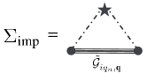
Figure S2: Diagrammatic representation of Eq. S64. The dotted line associated with a star represents the impurity potential, Eq. S62.

As a result, the frequency $z=iq_{n}-\delta\xi_{\textbf{q}}$ and the pairing gap $\Delta$ are renormalized in the full Green function $\tilde{\mathcal{G}}_{iq_{n},\textbf{q}}^{-1}={G}_{iq_{n},\textbf{q}}^{-1}-\Sigma_{\text{imp}}(iq_{n})$,

$$\tilde{\mathcal{G}}_{iq_{n},\textbf{q}}^{-1}=(i\tilde{q}_{n}-\delta\xi_{\textbf{q}})\tau^{0}-{\xi}_{\textbf{q}}\tau^{3}-\tilde{\Delta}\tau^{1},$$ (S65)

where

$$\tilde{z}(z)=z+in_{\text{imp}}u_{0}^{2}~{}\Gamma_{1}(\tilde{z},\tilde{\Delta})=z-n_{\text{imp}}u_{0}^{2}\int_{\textbf{q}}\frac{\tilde{z}}{\tilde{z}^{2}-\xi^{2}_{\textbf{q}}-\tilde{\Delta}^{2}},$$

$$\tilde{\Delta}(z)=\Delta+in_{\text{imp}}u_{0}^{2}~{}\Gamma_{2}(\tilde{z},\tilde{\Delta})=\Delta-n_{\text{imp}}u_{0}^{2}\int_{\textbf{q}}\frac{\tilde{\Delta}}{\tilde{z}^{2}-\xi^{2}_{\textbf{q}}-\tilde{\Delta}^{2}}.$$ (S66)

Since the real part of $\Sigma_{\text{imp}}(iq_{n}\rightarrow\omega+i\eta)$ yields energy shifts, we will only focus on the imaginary part. For large frequency $z$, both corrections are small, $\Gamma_{1}\approx 0$ and $\Gamma_{2}\approx 0$. The current-current correlation is (without the vertex correction),

$$P_{ij}(i\omega_{m})=-2e^{2}T\sum_{iq_{n}}\int_{\textbf{q}}v_{\textbf{q},i}v_{\textbf{q},j}\frac{\tilde{z}\tilde{z}_{+}+\xi_{\textbf{q}}^{2}+\tilde{\Delta}\tilde{\Delta}_{+}}{(\tilde{z}^{2}-\xi_{\textbf{q}}^{2}-\tilde{\Delta}^{2})(\tilde{z}_{+}^{2}-\xi_{\textbf{q}}^{2}-\tilde{\Delta}_{+}^{2})}$$ (S67)

where $\tilde{z}_{+}=\tilde{z}(z_{+})$, $\tilde{\Delta}_{+}=\tilde{\Delta}(z_{+})$ and $z_{+}=z+i\omega_{m}$. Using the contour integral, $\text{Im}P_{ij}(\omega+i\eta)$ can be simplified for large $\omega$. Each term in Eq. S67 can be written as

$$\mathcal{S}(i\omega_{m})=-T\sum_{iq_{n}}f_{1}(iq_{n})f_{2}(iq_{n}+i\omega_{m})=\oint_{\mathcal{C}}\frac{dz}{2\pi i}n_{F}(z)f_{1}(z)f_{2}(z+i\omega_{m}),$$ (S68)

for some functions $(f_{1,2}(E+i\eta))^{*}=f_{1,2}(E-i\eta)$ and the contour surrounds the branch cut at $z=E$ and $z=E-i\omega_{m}$ shown in Fig. S3,

$$\mathcal{S}(i\omega_{m}) = \int_{-\infty}^{\infty}\frac{dE}{2\pi i}\Big{[}n_{F}(E)\Big{(}f_{1}(E+i\eta)f_{2}(E+i\omega_{m})-f_{1}(E-i\eta)f_{2}(E+i\omega_{m})$$ (S69)

$$\qquad\qquad+f_{1}(E-i\omega_{m})f_{2}(E+i\eta)-f_{1}(E-i\omega_{m})f_{2}(E-i\eta)\Big{]}$$

and

$$\text{Im}\mathcal{S}(\omega+i\eta)=\int_{-\infty}^{\infty}\frac{dE}{\pi}\Big{(}n_{F}(E)-n_{F}(E+\omega)\Big{)}\text{Im}f_{1}(E+i\eta)~{}\text{Im}f_{2}(E+\omega+i\eta),$$ (S70)

where we used $2i\text{Im}f_{1,2}(E+i\eta)=f_{1,2}(E+i\eta)-f_{1,2}(E-i\eta)$. For large $\omega$,

$$P_{ij}(i\omega_{m}\rightarrow\omega+i\eta)\approx-\frac{4e^{2}}{\omega^{2}}T\sum_{iq_{n}}\int_{\textbf{q}}v_{\textbf{q},i}v_{\textbf{q},j}\frac{\tilde{z}\tilde{z}_{+}+\xi_{\textbf{q}}^{2}+\tilde{\Delta}\tilde{\Delta}_{+}}{\tilde{z}^{2}-\xi_{\textbf{q}}^{2}-\tilde{\Delta}^{2}}.$$ (S71)

At small $n_{\text{imp}}u_{0}^{2}$, the corrections in Eq. S66 are also small ($\tilde{z}\approx z$, $\tilde{\Delta}\approx\Delta$) and the disorder-mediated response at zero temperature can be obtained by using Eq. S70,

$$\text{Re}~{}\sigma_{\text{dis},ij}(\omega)=\frac{\text{Im}P_{ij}(\omega+i\eta)}{\omega}\approx\frac{e^{2}n_{\text{imp}}u_{0}^{2}\pi}{\omega^{3}}\int_{0}^{\omega}dE\Big{(}\int_{\textbf{q}}v_{\textbf{q},i}v_{\textbf{q},j}A(\textbf{q},E)\Big{)}\mathcal{D}(\omega-E)\Big{(}1-\frac{\Delta^{2}}{E(\omega-E)}\Big{)},$$ (S72)

where $A(\textbf{q},\omega)=-\frac{1}{\pi}\text{Tr}\text{Im}G_{\omega+i\eta,\textbf{q}}$ is the spectral function and $\mathcal{D}(\omega)=\int_{\textbf{q}}A(\textbf{q},\omega)$ is the density of state of superconductor. Even if the supercurrent is turned off $\textbf{Q}=0$, Eq. S72 is still finite, $\text{Re}~{}\sigma_{\text{dis},ij}(\omega)>0$ since the impurity potential Eq. S62 allows the indirect transitions. For the finite Q, the frequency threshold of $A(\textbf{q},\omega)$ is slightly reduced (Fig. 1b in the main text), thus $\text{Re}~{}\sigma_{\text{dis},ij}(\omega)$ is also finite just below the gap edge, $\omega\lesssim 2|\Delta|$.

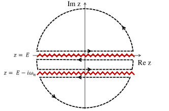
Figure S3: The contour $\mathcal{C}$ around two branch cuts $z=E$ and $z=E-i\omega_{m}$ to calculate the Mastubara sum in Eq. S67.

References

Van Hove [1953]L. Van Hove, The occurrence of
singularities in the elastic frequency distribution of a crystal, Phys. Rev. 89, 1189 (1953).
Lifshitz et al. [1960]I. Lifshitz et al., Anomalies
of electron characteristics of a metal in the high pressure region, Sov. Phys. JETP 11, 1130 (1960).
Ortiz et al. [2019]B. R. Ortiz, L. C. Gomes,
J. R. Morey, M. Winiarski, M. Bordelon, J. S. Mangum, I. W. H. Oswald, J. A. Rodriguez-Rivera, J. R. Neilson, S. D. Wilson, E. Ertekin, T. M. McQueen, and E. S. Toberer, New
kagome prototype materials: discovery of
, and
, Phys. Rev. Mater. 3, 094407 (2019).
Ratcliff et al. [2021]N. Ratcliff, L. Hallett,
B. R. Ortiz, S. D. Wilson, and J. W. Harter, Coherent phonon spectroscopy and interlayer modulation of
charge density wave order in the kagome metal
, Phys. Rev. Mater. 5, L111801 (2021).
Jiang et al. [2021]Y.-X. Jiang, J.-X. Yin,
M. M. Denner, N. Shumiya, B. R. Ortiz, G. Xu, Z. Guguchia, J. He, M. S. Hossain, X. Liu, J. Ruff, L. Kautzsch, S. S. Zhang, G. Chang, I. Belopolski, Q. Zhang, T. A. Cochran, D. Multer, M. Litskevich,
Z.-J. Cheng, X. P. Yang, Z. Wang, R. Thomale, T. Neupert, S. D. Wilson, and M. Z. Hasan, Unconventional
chiral charge order in kagome superconductor kv3sb5, Nature Materials 20, 1353 (2021).
Zhao et al. [2021]H. Zhao, H. Li, B. R. Ortiz, S. M. L. Teicher, T. Park, M. Ye, Z. Wang, L. Balents,
S. D. Wilson, and I. Zeljkovic, Cascade of correlated electron states in the
kagome superconductor csv3sb5, Nature 599, 216 (2021).
Duan et al. [2021]W. Duan, Z. Nie, S. Luo, F. Yu, B. R. Ortiz, L. Yin, H. Su, F. Du, A. Wang, Y. Chen, X. Lu, J. Ying, S. D. Wilson,
X. Chen, Y. Song, and H. Yuan, Nodeless superconductivity in the kagome metal csv3sb5, Science China Physics, Mechanics & Astronomy 64, 107462 (2021).
Xiang et al. [2021]Y. Xiang, Q. Li, Y. Li, W. Xie, H. Yang, Z. Wang, Y. Yao, and H.-H. Wen, Twofold symmetry of c-axis resistivity in
topological kagome superconductor csv3sb5 with in-plane rotating magnetic
field, Nature Communications 12, 6727 (2021).
Li et al. [2021]H. Li, T. T. Zhang,
T. Yilmaz, Y. Y. Pai, C. E. Marvinney, A. Said, Q. W. Yin, C. S. Gong, Z. J. Tu, E. Vescovo,
C. S. Nelson, R. G. Moore, S. Murakami, H. C. Lei, H. N. Lee, B. J. Lawrie, and H. Miao, Observation of unconventional charge density wave without acoustic phonon
anomaly in kagome superconductors
(, cs), Phys. Rev. X 11, 031050 (2021).
Ortiz et al. [2021]B. R. Ortiz, S. M. L. Teicher, L. Kautzsch,
P. M. Sarte, N. Ratcliff, J. Harter, J. P. C. Ruff, R. Seshadri, and S. D. Wilson, Fermi surface mapping and the nature of charge-density-wave order in the
kagome superconductor , Phys. Rev. X 11, 041030 (2021).
Tan et al. [2021]H. Tan, Y. Liu, Z. Wang, and B. Yan, Charge density waves and electronic properties of superconducting
kagome metals, Phys. Rev. Lett. 127, 046401 (2021).
Neupert et al. [2022]T. Neupert, M. M. Denner,
J.-X. Yin, R. Thomale, and M. Z. Hasan, Charge order and superconductivity in kagome materials, Nature Physics 18, 137 (2022).
Hu et al. [2022]Y. Hu, X. Wu, B. R. Ortiz, S. Ju, X. Han, J. Ma, N. C. Plumb,
M. Radovic, R. Thomale, S. D. Wilson, A. P. Schnyder, and M. Shi, Rich nature of van hove singularities in kagome superconductor
csv3sb5, Nature Communications 13, 2220 (2022).
Scammell et al. [2023]H. D. Scammell, J. Ingham,
T. Li, and O. P. Sushkov, Chiral excitonic order from twofold van hove
singularities in kagome metals, Nature Communications 14, 605 (2023).
Kim et al. [2016]Y. Kim, P. Herlinger,
P. Moon, M. Koshino, T. Taniguchi, K. Watanabe, and J. H. Smet, Charge
inversion and topological phase transition at a twist angle induced van hove
singularity of bilayer graphene, Nano Letters 16, 5053 (2016), pMID:
27387484, https://doi.org/10.1021/acs.nanolett.6b01906 .
Yan et al. [2012]W. Yan, M. Liu, R.-F. Dou, L. Meng, L. Feng, Z.-D. Chu, Y. Zhang, Z. Liu, J.-C. Nie, and L. He, Angle-dependent van hove singularities in a slightly twisted
graphene bilayer, Phys. Rev. Lett. 109, 126801 (2012).
Schouteden et al. [2016]K. Schouteden, Z. Li,
T. Chen, F. Song, B. Partoens, C. Van Haesendonck, and K. Park, Moiré
superlattices at the topological insulator bi2te3, Scientific Reports 6, 20278 (2016).
Brihuega et al. [2012]I. Brihuega, P. Mallet,
H. González-Herrero,
G. Trambly de
Laissardière, M. M. Ugeda, L. Magaud,
J. M. Gómez-Rodríguez, F. Ynduráin, and J.-Y. Veuillen, Unraveling the intrinsic
and robust nature of van hove singularities in twisted bilayer graphene by
scanning tunneling microscopy and theoretical analysis, Phys. Rev. Lett. 109, 196802 (2012).
Classen et al. [2019]L. Classen, C. Honerkamp, and M. M. Scherer, Competing phases of interacting
electrons on triangular lattices in moiré heterostructures, Phys. Rev. B 99, 195120 (2019).
Lin and Nandkishore [2019]Y.-P. Lin and R. M. Nandkishore, Chiral twist on the
high- phase diagram in moiré heterostructures, Phys. Rev. B 100, 085136 (2019).
Li et al. [2010]G. Li, A. Luican, J. M. B. Lopes dos Santos,
A. H. Castro Neto,
A. Reina, J. Kong, and E. Y. Andrei, Observation of van hove singularities in twisted graphene
layers, Nature Physics 6, 109 (2010).
Luican et al. [2011]A. Luican, G. Li, A. Reina, J. Kong, R. R. Nair, K. S. Novoselov, A. K. Geim, and E. Y. Andrei, Single-layer
behavior and its breakdown in twisted graphene layers, Phys. Rev. Lett. 106, 126802 (2011).
Yan et al. [2014]W. Yan, L. Meng, M. Liu, J.-B. Qiao, Z.-D. Chu, R.-F. Dou, Z. Liu, J.-C. Nie, D. G. Naugle, and L. He, Angle-dependent van hove singularities
and their breakdown in twisted graphene bilayers, Phys. Rev. B 90, 115402 (2014).
Liao et al. [2015]L. Liao, H. Wang, H. Peng, J. Yin, A. L. Koh, Y. Chen, Q. Xie, H. Peng, and Z. Liu, van hove singularity enhanced photochemical
reactivity of twisted bilayer graphene, Nano Letters 15, 5585 (2015).
Yin et al. [2016]J. Yin, H. Wang, H. Peng, Z. Tan, L. Liao, L. Lin, X. Sun, A. L. Koh, Y. Chen, H. Peng, and Z. Liu, Selectively
enhanced photocurrent generation in twisted bilayer graphene with van hove
singularity, Nature Communications 7, 10699 (2016).
Cao et al. [2018a]Y. Cao, V. Fatemi,
S. Fang, K. Watanabe, T. Taniguchi, E. Kaxiras, and P. Jarillo-Herrero, Unconventional superconductivity in magic-angle graphene
superlattices, Nature 556, 43 (2018a).
Cao et al. [2018b]Y. Cao, V. Fatemi,
A. Demir, S. Fang, S. L. Tomarken, J. Y. Luo, J. D. Sanchez-Yamagishi, K. Watanabe, T. Taniguchi, E. Kaxiras, R. C. Ashoori, and P. Jarillo-Herrero, Correlated insulator behaviour at half-filling in magic-angle graphene
superlattices, Nature 556, 80 (2018b).
Kerelsky et al. [2019]A. Kerelsky, L. J. McGilly, D. M. Kennes,
L. Xian, M. Yankowitz, S. Chen, K. Watanabe, T. Taniguchi, J. Hone, C. Dean, A. Rubio, and A. N. Pasupathy, Maximized electron interactions at the
magic angle in twisted bilayer graphene, Nature 572, 95 (2019).
Xie et al. [2019]Y. Xie, B. Lian, B. Jäck, X. Liu, C.-L. Chiu, K. Watanabe, T. Taniguchi, B. A. Bernevig, and A. Yazdani, Spectroscopic signatures of many-body correlations in magic-angle twisted
bilayer graphene, Nature 572, 101 (2019).
Nimbalkar and Kim [2020]A. Nimbalkar and H. Kim, Opportunities and challenges
in twisted bilayer graphene: A review, Nano-Micro Letters 12, 126 (2020).
Xu et al. [2021]S. Xu, M. M. Al Ezzi,
N. Balakrishnan, A. Garcia-Ruiz, B. Tsim, C. Mullan, J. Barrier, N. Xin, B. A. Piot, T. Taniguchi, K. Watanabe,
A. Carvalho, A. Mishchenko, A. K. Geim, V. I. Fal’ko, S. Adam, A. H. C. Neto, K. S. Novoselov, and Y. Shi, Tunable van
hove singularities and correlated states in twisted monolayer–bilayer
graphene, Nature Physics 17, 619 (2021).
Chichinadze et al. [2022]D. V. Chichinadze, L. Classen, Y. Wang, and A. V. Chubukov, Cascade of transitions in twisted and
non-twisted graphene layers within the van hove scenario, npj Quantum Materials 7, 114 (2022).
Zhang et al. [2023]Y. Zhang, R. Polski,
A. Thomson, É. Lantagne-Hurtubise, C. Lewandowski, H. Zhou, K. Watanabe, T. Taniguchi, J. Alicea, and S. Nadj-Perge, Enhanced superconductivity in spin–orbit proximitized bilayer graphene, Nature 613, 268 (2023).
Nandkishore et al. [2012a]R. Nandkishore, L. S. Levitov, and A. V. Chubukov, Chiral superconductivity
from repulsive interactions in doped graphene, Nature Physics 8, 158 (2012a).
Nandkishore et al. [2012b]R. Nandkishore, G.-W. Chern, and A. V. Chubukov, Itinerant half-metal
spin-density-wave state on the hexagonal lattice, Phys. Rev. Lett. 108, 227204 (2012b).
Hsu et al. [2020]Y.-T. Hsu, F. Wu, and S. Das Sarma, Topological superconductivity, ferromagnetism, and
valley-polarized phases in moiré systems: Renormalization group analysis
for twisted double bilayer graphene, Phys. Rev. B 102, 085103 (2020).
Wang et al. [2021a]T. Wang, N. F. Q. Yuan, and L. Fu, Moiré surface states and enhanced
superconductivity in topological insulators, Phys. Rev. X 11, 021024 (2021a).
Lin and Nandkishore [2018]Y.-P. Lin and R. M. Nandkishore, Kohn-luttinger
superconductivity on two orbital honeycomb lattice, Phys. Rev. B 98, 214521 (2018).
Chichinadze et al. [2020]D. V. Chichinadze, L. Classen, and A. V. Chubukov, Valley magnetism,
nematicity, and density wave orders in twisted bilayer graphene, Phys. Rev. B 102, 125120 (2020).
Hsu et al. [2021]Y.-T. Hsu, F. Wu, and S. Das Sarma, Spin-valley locked instabilities in moiré
transition metal dichalcogenides with conventional and higher-order van hove
singularities, Phys. Rev. B 104, 195134 (2021).
Park et al. [2021]T. Park, M. Ye, and L. Balents, Electronic instabilities of kagome metals: Saddle
points and landau theory, Phys. Rev. B 104, 035142 (2021).
Hur and Maurice
Rice [2009]K. L. Hur and T. Maurice
Rice, Superconductivity close to
the mott state: From condensed-matter systems to superfluidity in optical
lattices, Annals of Physics 324, 1452 (2009), july 2009 Special Issue.
Nandkishore and Chubukov [2012]R. Nandkishore and A. V. Chubukov, Interplay of
superconductivity and spin-density-wave order in doped graphene, Phys. Rev. B 86, 115426 (2012).
Classen et al. [2020]L. Classen, A. V. Chubukov, C. Honerkamp, and M. M. Scherer, Competing orders at
higher-order van hove points, Phys. Rev. B 102, 125141 (2020).
Rømer et al. [2022]A. T. Rømer, S. Bhattacharyya, R. Valentí, M. H. Christensen, and B. M. Andersen, Superconductivity from
repulsive interactions on the kagome lattice, Phys. Rev. B 106, 174514 (2022).
Shtyk et al. [2017]A. Shtyk, G. Goldstein, and C. Chamon, Electrons at the monkey saddle: A
multicritical lifshitz point, Phys. Rev. B 95, 035137 (2017).
Kozii et al. [2019]V. Kozii, H. Isobe,
J. W. F. Venderbos, and L. Fu, Nematic superconductivity stabilized by density
wave fluctuations: Possible application to twisted bilayer graphene, Phys. Rev. B 99, 144507 (2019).
Isobe et al. [2018]H. Isobe, N. F. Q. Yuan, and L. Fu, Unconventional superconductivity and density waves
in twisted bilayer graphene, Phys. Rev. X 8, 041041 (2018).
Lin and Nandkishore [2021]Y.-P. Lin and R. M. Nandkishore, Complex charge
density waves at van hove singularity on hexagonal lattices: Haldane-model
phase diagram and potential realization in the kagome metals
(=k, rb, cs), Phys. Rev. B 104, 045122 (2021).
Ramires et al. [2012]A. Ramires, P. Coleman,
A. H. Nevidomskyy, and A. M. Tsvelik, : A
critical nodal metal, Phys. Rev. Lett. 109, 176404 (2012).
Lin and Nandkishore [2020]Y.-P. Lin and R. M. Nandkishore, Parquet
renormalization group analysis of weak-coupling instabilities with multiple
high-order van hove points inside the brillouin zone, Phys. Rev. B 102, 245122 (2020).
Efremov et al. [2019]D. V. Efremov, A. Shtyk,
A. W. Rost, C. Chamon, A. P. Mackenzie, and J. J. Betouras, Multicritical fermi surface topological transitions, Phys. Rev. Lett. 123, 207202 (2019).
Jeong et al. [2022]M. Y. Jeong, H.-J. Yang,
H. S. Kim, Y. B. Kim, S. Lee, and M. J. Han, Crucial role of out-of-plane sb orbitals in van hove singularity
formation and electronic correlations in the superconducting kagome metal
, Phys. Rev. B 105, 235145 (2022).
Julku et al. [2016]A. Julku, S. Peotta,
T. I. Vanhala, D.-H. Kim, and P. Törmä, Geometric origin of superfluidity in the lieb-lattice flat band, Phys. Rev. Lett. 117, 045303 (2016).
Liang et al. [2017a]L. Liang, T. I. Vanhala,
S. Peotta, T. Siro, A. Harju, and P. Törmä, Band geometry, berry curvature, and superfluid weight, Phys. Rev. B 95, 024515 (2017a).
Liang et al. [2017b]L. Liang, S. Peotta,
A. Harju, and P. Törmä, Wave-packet dynamics of bogoliubov quasiparticles: Quantum
metric effects, Phys. Rev. B 96, 064511 (2017b).
Ahn and Nagaosa [2021a]J. Ahn and N. Nagaosa, Superconductivity-induced spectral
weight transfer due to quantum geometry, Phys. Rev. B 104, L100501 (2021a).
Wang et al. [2021b]Z. Wang, L. Dong, C. Xiao, and Q. Niu, Berry curvature effects on quasiparticle dynamics in
superconductors, Phys. Rev. Lett. 126, 187001 (2021b).
Liao and Hsu [2023]Y. Liao and Y.-T. Hsu, Unveiling quasiparticle berry
curvature effects in the spectroscopic properties of a chiral p-wave
superconductor, arXiv preprint arXiv:2311.02165 (2023).
Karecki et al. [1982]D. Karecki, R. E. Peña, and S. Perkowitz, Far-infrared
transmission of superconducting homogeneous nbn films: Scattering time
effects, Phys. Rev. B 25, 1565 (1982).
Somal et al. [1996]H. S. Somal, B. J. Feenstra,
J. Schützmann, J. Hoon Kim, Z. H. Barber, V. H. M. Duijn, N. T. Hien, A. A. Menovsky, M. Palumbo, and D. van der Marel, Grazing incidence infrared reflectivity of
and nbn, Phys. Rev. Lett. 76, 1525 (1996).
Cheng et al. [2016]B. Cheng, L. Wu, N. J. Laurita, H. Singh, M. Chand, P. Raychaudhuri, and N. P. Armitage, Anomalous gap-edge dissipation in disordered superconductors on the brink of
localization, Phys. Rev. B 93, 180511 (2016).
Seibold et al. [2017]G. Seibold, L. Benfatto, and C. Castellani, Application of the mattis-bardeen
theory in strongly disordered superconductors, Phys. Rev. B 96, 144507 (2017).
Uzawa et al. [2020]Y. Uzawa, S. Saito,
W. Qiu, K. Makise, T. Kojima, and Z. Wang, Optical
and tunneling studies of energy gap in superconducting niobium nitride
films, Journal of Low Temperature Physics 199, 143 (2020).
Nakamura et al. [2019]S. Nakamura, Y. Iida,
Y. Murotani, R. Matsunaga, H. Terai, and R. Shimano, Infrared activation of the higgs mode by supercurrent injection in
superconducting nbn, Phys. Rev. Lett. 122, 257001 (2019).
Nakamura et al. [2020]S. Nakamura, K. Katsumi,
H. Terai, and R. Shimano, Nonreciprocal terahertz second-harmonic generation in
superconducting nbn under supercurrent injection, Phys. Rev. Lett. 125, 097004 (2020).
Xu et al. [2019]T. Xu, T. Morimoto, and J. E. Moore, Nonlinear optical effects in
inversion-symmetry-breaking superconductors, Phys. Rev. B 100, 220501 (2019).
[81] See Supplementary Materials at URL for
details on I. Galilean invariance, II. Optical conductivity calculations,
III. Peak intensity and IV. Effect of disorder with Refs
[89, 80, 84, 85, 39, 82].
Bruus and Flensberg [2004]H. Bruus and K. Flensberg, Many-body quantum
theory in condensed matter physics: an introduction (OUP Oxford, 2004).
Note [1]The Ward identity has the form
where .
Schrieffer [2018]J. R. Schrieffer, Theory of
superconductivity (CRC press, 2018).
Burganov et al. [2016]B. Burganov, C. Adamo,
A. Mulder, M. Uchida, P. D. C. King, J. W. Harter, D. E. Shai, A. S. Gibbs, A. P. Mackenzie, R. Uecker, M. Bruetzam, M. R. Beasley, C. J. Fennie, D. G. Schlom, and K. M. Shen, Strain control
of fermiology and many-body interactions in two-dimensional ruthenates, Phys. Rev. Lett. 116, 197003 (2016).
Hsu et al. [2016]Y.-T. Hsu, W. Cho, A. F. Rebola, B. Burganov, C. Adamo, K. M. Shen, D. G. Schlom, C. J. Fennie, and E.-A. Kim, Manipulating
superconductivity in ruthenates through fermi surface engineering, Phys. Rev. B 94, 045118 (2016).
Gottfried [2018]K. Gottfried, Quantum mechanics:
fundamentals (CRC Press, 2018).