Signatures of fragmentation for periodically driven fermions

Abstract

We study the possible signatures of prethermal strong Hilbert space fragmentation (HSF) for one-dimensional (1D) fermions subjected to a periodic drive. We extend the results of Phys. Rev. Lett. 130, 120401 (2023) to show the possibility of such fragmentation for a large class of experimentally relevant drive protocols. Moreover, we demonstrate the persistence of HSF when the fermion chain is taken away from half-filling. Both these analysis indicate the robustness of the fragmentation phenomenon reported earlier. We also provide an alternate derivation of the Floquet Hamiltonian of the driven chain which yields insight into the generic nested commutator structure of its higher order terms. Finally, we study the density-density out-of-time-correlators (OTOC) of the driven chain both away and near the special drive frequencies at which its first order Floquet Hamiltonian exhibits fragmentation. We show that these OTOCs, for a chain with open boundary condition, exhibit a distinct periodic unscrambling of information at special drive frequencies; such unscrambling can therefore serve as a marker of prethermal HSF. We provide an approximate analytic explanation of the role of HSF behind such periodic unscrambling and discuss experiments which can detect signatures of strong HSF in such driven chains.

I Introduction

Closed quantum systems driven out of equilibrium have become increasingly important subject of research in recent years [1, 2, 3]. One of the central questions in this field pertains to the long-time behavior of local correlation functions of these systems. In most case, the behavior of such correlation functions can be understood from the eigenstate thermalization hypothesis (ETH) [4, 5]. ETH predicts eventual thermalization, under unitary Hamiltonian dynamics, of a generic many-body quantum state which can initially be far from equilibrium; it is one of the central paradigms for understanding long-time behavior of a generic ergodic many-body system. ETH also holds, with minor modifications, for periodically driven systems, where the driven system is ultimately expected to heat up to infinite temperature [6].

ETH relies on the ergodicity of a generic quantum system and is known to fail when it is violated. Such ergodicity violation can occur in integrable models due to the presence of a large number of conserved quantities [1]. In addition, it fails in the presence of strong disorder leading to many-body localization and consequent violation of ergodicity [7, 8, 9]. A more subtle and weaker failure of ETH occurs due to emergent symmetry sectors in an otherwise generic quantum systems. The presence of such symmetries typically lead to tower of states which are protected from the other thermal states in its Hilbert space. Thus any quantum dynamics starting from an initial state which belongs to this sectors can not thermalize; such states are often called quantum scars [10, 11, 12, 13, 14]. The violation of ETH in this case is weak since it only happens if the initial state has large overlap with the states in the scar sector. The number of such states, for a one-dimensional (1D) system of length $L$, is typically ${\rm O}(L)$; they form a tiny fraction of the total number of states in the Hilbert space which is ${\rm O}(e^{L})$. Thus these systems display ETH violating dynamics for a small fraction of initial states.

Another, recently found, violation of ETH occurs in non-integrable quantum systems due to the presence of kinetic constraints. The Hamiltonian of such quantum systems, expressed as a matrix in the computational basis, breaks down into an exponentially large number of dynamically disconnected fragments. The presence of such a large number of disconnected sectors is to be contrasted with those occurring from the presence of conserved global quantities; the latter only leads to an ${\rm O}(L)$ disconnected symmetry sectors. This phenomenon is known as strong Hilbert space fragmentation (HSF) [15, 16, 17, 18, 19]. Such a strong fragmentation naturally breaks ergodicity since any generic initial state, which belongs to a given fragment, can not, under the action of the system Hamiltonian, explore states in the Hilbert space that belong to other fragments. Most of the Hamiltonians studied in this context are 1D spin or fermionic models [15, 16, 17, 18]; however, more recently some higher-dimensional models have also been shown to exhibit strong HSF [19].

More recently, the generalization of strong HSF to periodically driven quantum system has been studied [20]. It has been shown that a periodically driven fermionic chain can show signatures of Hilbert space fragmentation at special drive frequencies over a large prethermal timescale; the extent of this prethermal timescale depends on the drive amplitude and can be quite large in the large drive amplitude regime. The signatures of such prethermal fragmentation can be found in entanglement entropy, autocorrelation function and equal-time correlators of such driven system; each of these quantities show departure from their counterparts in ergodic quantum systems [20] demonstrating a clear realization of prethermal strong HSF. In addition, such prethermal HSF in driven quantum systems can lead to interesting oscillatory dynamics of correlators for certain initial states which has no counterpart for HSF realized in an equilibrium setting [20].

In this work, we extend the results obtained in Ref. 20 in several ways. First, we show that such signatures of fragmentation can be obtained for a much wider class of drive protocols. This makes the prethermal fragmentation phenomenon much more relevant to standard experiments using ultracold atom platform which we discuss. Second, we provide a comprehensive analysis of the Floquet Hamiltonian. The analytical expression for the first order Floquet Hamiltonian, $H_{F}^{(1)}$, derived using Floquet perturbation theory (FPT), was presented in Ref. 20; here we provide an alternate derivation of the Floquet Hamiltonian up to second order in perturbation theory. This analysis provides insight into the commutator structure of the higher order terms that was not apparent from the previous derivation. It also provides an estimate of the frequency range over which the first order Floquet Hamiltonian provides a qualitatively accurate description of the dynamical evolution in the prethermal regime. Third, we show that the signature of fragmentation persists when the driven chain is taken away from half-filling. This shows the robustness of the prethermal fragmentation phenomenon and points out the possibility of its experimental realization for a wide range of fermion filling fraction. Finally, we study the density-density out-of-time correlator (OTOC) for the driven fermion chain. We show that the behavior of such OTOC is qualitatively different at special frequencies at which the system exhibits signatures of prethermal HSF. In particular, for a driven fermion chain with open boundary condition, we find, starting from a initial ${\mathbb{Z}}_{2}$ state, unscrambling of information manifested through periodic revival of the OTOC. We analyze this phenomenon in details, provide an analytic, albeit qualitative, understanding of its mechanism, and tie it to the fragmented structure of the first-order Floquet Hamiltonian, $H_{F}^{(1)}$, of the driven chain obtained using FPT. Our results thus demonstrate that OTOCs can server as markers for prethermal HSF in a driven system.

The organization of the rest of this work is as follows. In Sec. II, we present a derivation of the Floquet Hamiltonian which brings out its nested commutator structure. Next, in Sec. III, we discuss the different classes of drive protocols which allows for signature of prethermal fragmentation and also derive the higher order Floquet Hamiltonian corresponding to them. This is followed by Sec. IV where we demonstrate signature of prethermal HSF away from half-filling. Next, in Sec. V, we discuss the behavior of OTOC in such driven system. Finally, we discuss our main results and conclude in Sec. VI. Some details of the calculation are presented in the Appendices.

II Formalism

In this section, we outline the derivation of the Floquet Hamiltonian of the driven fermion chain. Our derivation brings out the nested commutator structure of the Floquet Hamiltonian and also addresses a more general class of drive protocols for which the fermion chain exhibits prethermal HSF.

II.1 Preliminary

Consider a time dependent quantum mechanical system described by the Hamiltonian

$$\mathcal{H}(t)=\mathcal{H}_{0}(t)+\mathcal{H}_{1},$$ (1)

where all the time dependence is in the zeroth order term $\mathcal{H}_{0}$. The term $\mathcal{H}_{1}$, which in the following will be treated perturbatively, has no explicit time dependence. From Schrodinger equation $i\hbar\partial_{t}\psi(t)=[\mathcal{H}_{0}(t)+\mathcal{H}_{1}]\psi(t)$, and the definition of the time evolution operator $U(t,0)$ via $\psi(t)=U(t,0)\psi(0)$, we get

$$i\hbar\frac{\partial}{\partial t}U(t,0)=[\mathcal{H}_{0}(t)+\mathcal{H}_{1}]U(t,0).$$ (2)

The evaluation of $U(t,0)$ can be broken into two steps. To do so, we write [21, 22, 23]

$$U(t,0)=U_{0}(t,0)W(t,0),$$ (3)

where $U_{0}(t,0)$ is the exact time evolution operator in the absence of the $\mathcal{H}_{1}$ term. The first step, which is simple, is to evaluate $U_{0}(t,0)$ which is given by

$$U_{0}(t,0)=\exp[-\frac{i}{\hbar}\int_{0}^{t}d\tau\mathcal{H}_{0}(\tau)].$$ (4)

In the above the time ordering in front of the exponential can be omitted since the operator $\mathcal{H}_{0}(\tau)$ at different times commute. The second step, which is non-trivial, is to compute $W(t,0)$ that encodes the time evolution due to $\mathcal{H}_{1}$. This is performed perturbatively. Using $i\partial_{t}U_{0}(t,0)=\mathcal{H}_{0}U_{0}(t,0)$ and Eqs. (2) and (3), we get

$$i\hbar\frac{\partial}{\partial t}W(t,0)=\mathcal{H}_{p}(t)W(t,0),$$ (5)

where

$$\mathcal{H}_{p}(t)\equiv U_{0}(t,0)^{-1}\mathcal{H}_{1}U_{0}(t,0).$$ (6)

Using Eq. (5), the perturbative expansion is

$$W(t,0) =1-\left(\frac{i}{\hbar}\right)\int_{0}^{t}d\tau\mathcal{H}_{p}(\tau)\,+$$

$$\left(-\frac{i}{\hbar}\right)^{2}\int_{0}^{t}d\tau_{1}\mathcal{H}_{p}(\tau_{1})\int_{0}^{\tau_{1}}d\tau_{2}\mathcal{H}_{p}(\tau_{2})\,+$$

$$\left(-\frac{i}{\hbar}\right)^{3}\!\int_{0}^{t}\!d\tau_{1}\mathcal{H}_{p}(\tau_{1})\int_{0}^{\tau_{1}}\!d\tau_{2}\mathcal{H}_{p}(\tau_{2})\int_{0}^{\tau_{2}}\!d\tau_{3}\mathcal{H}_{p}(\tau_{3})$$

$$+\cdots.$$ (7)

Note, in the above the operator $\mathcal{H}_{p}(\tau)$ at different times do not commute.

The above formulation can also be viewed as a series expansion in a rotating frame for the following reason. Consider a time dependent unitary transformation $V(t)$ between a laboratory to a rotating reference frame with the initial condition $V(0)=1$. The wavefunction in the rotating frame is $\psi_{r}(t)=V^{\dagger}(t)\psi(t)$, and an operator in the same frame is $\mathcal{O}_{r}(t)=V^{\dagger}(t)\mathcal{O}V(t)$, where $\psi(t)$ and $\mathcal{O}$ are the wavefunction and the operator in the laboratory frame, respectively. Simultaneously, the Hamiltonian $\mathcal{H}(t)$ in the laboratory frame transforms to $\mathcal{H}_{r}(t)$ in the rotating frame. By demanding that $i\hbar\partial_{t}\psi_{r}(t)=\mathcal{H}_{r}(t)\psi_{r}(t)$ we get

$$\mathcal{H}_{r}(t)=V^{\dagger}(t)\mathcal{H}(t)V(t)-i\hbar V^{\dagger}(t)\dot{V}(t),$$ (8)

where $\dot{V}\equiv\partial_{t}V(t)$. Furthermore, if we define the time evolution operator $U_{r}(t_{1},t_{2})$ in the rotating frame by $i\hbar\partial_{t_{1}}U_{r}(t_{1},t_{2})=\mathcal{H}_{r}(t_{1})U_{r}(t_{1},t_{2})$, then it is related to that in the laboratory frame by

$$U(t_{1},t_{2})=V(t_{1})U_{r}(t_{1},t_{2})V^{\dagger}(t_{2}).$$ (9)

The connection between the two formulations is made if we choose the time dependent unitary transformation to be

$$V(t)=\exp[-\frac{i}{\hbar}\int_{0}^{t}d\tau\mathcal{H}_{0}(\tau)],$$ (10)

such that the $\mathcal{H}_{0}(t)$ term is “gauged out” in the rotating frame. In this case $\mathcal{H}_{r}(t)$ coincides with $\mathcal{H}_{p}(t)$ given by Eq. (6), $U_{r}(t,0)$ with $W(t,0)$, and Eqs. (3) and (9) become identical with $t_{2}=0$.

However, note that the first formulation is more versatile in the sense that it can be still used when $\mathcal{H}_{1}$ is the zeroth order term and $\mathcal{H}_{0}$ is perturbative. In this case, we simply exchange $\mathcal{H}_{0}(t)\leftrightarrow\mathcal{H}_{1}$ in Eqs. (4) and (6). The resulting expansion will not match with that in the rotating frame.

II.2 Floquet perturbation theory

Until now the discussion has been general, and it applies to all time dependent problems. In the particular case of a Floquet system, where the time dependence is due a periodic external drive, we are interested in the stroboscopic time evolution operator $U(T,0)$, where $T$ is the period of the drive. The related Floquet Hamiltonian is defined by

$$\mathcal{H}_{F}\equiv\frac{i\hbar}{T}\log U(T,0)=\frac{i\hbar}{T}\log[U_{0}(T,0)W(T,0)].$$ (11)

We suppose that there is a small parameter that justifies the expansion $W(T,)=1+W_{1}(T)+W_{2}(T)+\cdots$, and correspondingly $\mathcal{H}_{F}=\mathcal{H}_{F}^{(0)}+\mathcal{H}_{F}^{(1)}+\mathcal{H}_{F}^{(2)}+\cdots$. Then, using Eq. (II.1) and after some algebra the first few terms in the expansion of the Floquet Hamiltonian are given by

$$\mathcal{H}_{F}^{(0)} =\frac{i\hbar}{T}\log U_{0}(T,0),$$ (12)

$$\mathcal{H}_{F}^{(1)} =\frac{i\hbar}{T}W_{1}(T)=\frac{1}{T}\int_{0}^{T}d\tau\mathcal{H}_{p}(\tau),$$ (13)

$$\mathcal{H}_{F}^{(2)} =\frac{i\hbar}{T}\left[W_{2}(T)-\frac{1}{2}W_{1}(T)^{2}\right]$$

$$=\frac{-i}{2\hbar T}\int_{0}^{T}d\tau_{1}\int_{0}^{\tau_{1}}d\tau_{2}\left[\mathcal{H}_{p}(\tau_{1}),\mathcal{H}_{p}(\tau_{2})\right],$$ (14)

$$\mathcal{H}_{F}^{(3)} =\frac{i\hbar}{T}\left[W_{3}(T)-\frac{1}{2}\left(W_{1}(T)W_{2}(T)+W_{2}(T)W_{1}(T)\right)\right.$$

$$+\left.\frac{1}{3}W_{1}(T)^{3}\right]$$

$$=-\frac{1}{6\hbar^{2}T}\int_{0}^{T}d\tau_{1}\int_{0}^{\tau_{1}}d\tau_{2}\int_{0}^{\tau_{2}}d\tau_{3}\left\{\left[\mathcal{H}_{p}(\tau_{1}),\right.\right.$$

$$\left.\left.\left[\mathcal{H}_{p}(\tau_{2}),\mathcal{H}_{p}(\tau_{3})\right]\right]+\left[\left[\mathcal{H}_{p}(\tau_{1}),\mathcal{H}_{p}(\tau_{2})\right],\mathcal{H}_{p}(\tau_{3})\right]\right\}.$$ (15)

Eqs. 12-15 indicate the nested commutator structure of the higher-order terms of the Floquet Hamiltonian; we shall use them for explicit computation of $H_{F}$ in Sec. III.

III Computation of the Floquet Hamiltonian

In this section we first provide analytical results for higher order terms in the Floquet Hamiltonian for a cosine drive protocol in Sec. III.1. This is followed, in Sec. III.2, by a derivation and analysis of the first order Floquet Hamiltonian $H_{F}^{(1)}$ for a more general drive protocol.

III.1 Cosine modulation of interaction

Consider a driven system described by Eq. (1) where

$$\mathcal{H}_{0}(t) =V_{1}\cos\omega_{D}t\sum_{i}\hat{n}_{i}\hat{n}_{i+1},$$ (16)

$$\mathcal{H}_{1} =\sum_{i}\left[-J(c^{\dagger}_{i}c_{i+1}+\rm{h.c.})+V_{0}\hat{n}_{i}\hat{n}_{i+1}+V_{2}\hat{n}_{i}\hat{n}_{i+2}\right],$$ (17)

with $V_{1}\gg(J,V_{0},V_{2})$. Thus, in the following we treat the $\mathcal{H}_{0}$ term exactly, and $\mathcal{H}_{1}$ perturbatively.

Following Sec. II, we have, using Eq. (4),

$$U_{0}(t,0)=\exp[-i\lambda\hat{B}\sin\omega_{D}t],$$ (18)

where $\lambda\equiv V_{1}/(\hbar\omega_{D})$ is a dimensionless parameter and $\hat{B}\equiv\sum_{j}\hat{n}_{j}\hat{n}_{j+1}$.

The next step is to compute $\mathcal{H}_{p}(t)$ using Eq. (6). As an intermediate step we find

$$\left[\hat{B},\mathcal{H}_{1}\right] =-J\sum_{i}\hat{A}_{i}\left(c^{\dagger}_{i}c_{i+1}-c^{\dagger}_{i+1}c_{i}\right),$$ (19)

$$\left[\hat{B},\left[\hat{B},\mathcal{H}_{1}\right]\right] =-J\sum_{i}\hat{A}_{i}^{2}\left(c^{\dagger}_{i}c_{i+1}+c^{\dagger}_{i+1}c_{i}\right),$$ (20)

and so on, where

$$\hat{A}_{i}=\hat{n}_{i-1}-\hat{n}_{i+2}.$$ (21)

. Using these relations we obtain

$$\mathcal{H}_{p}(t) =\exp[i\lambda\hat{B}\sin\omega_{D}t]\mathcal{H}_{1}\exp[-i\lambda\hat{B}\sin\omega_{D}t]$$

$$=\mathcal{H}_{1}+i\lambda\sin\omega_{D}t\left[\hat{B},\mathcal{H}_{1}\right]+\frac{1}{2!}(i\lambda\sin\omega_{D}t)^{2}$$

$$\times\left[\hat{B},\left[\hat{B},\mathcal{H}_{1}\right]\right]+\frac{1}{3!}(i\lambda\sin\omega_{D}t)^{3}\left[\hat{B},\left[\hat{B},\left[\hat{B},\mathcal{H}_{1}\right]\right]\right]$$

$$+\cdots$$

$$=\sum_{i}\left[-J\left(e^{i\lambda\hat{A}_{i}\sin\omega_{D}t}c^{\dagger}_{i}c_{i+1}+e^{-i\lambda\hat{A}_{i}\sin\omega_{D}t}c^{\dagger}_{i+1}c_{i}\right)\right.$$

$$\left.+V_{0}\hat{n}_{i}\hat{n}_{i+1}+V_{2}\hat{n}_{i}\hat{n}_{i+2}\right].$$ (22)

Using the explicit form of $\mathcal{H}_{p}(t)$ it is possible to compute order by order the Floquet Hamiltonian.

The zeroth order Floquet Hamiltonian $\mathcal{H}_{F}^{(0)}$ vanishes because, from Eq. (18), we have $U_{0}(T,0)=1$.

To compute the first order Floquet Hamiltonian we use the relation

$$I_{1}(\hat{A},\lambda) \equiv\frac{1}{T}\int_{0}^{T}d\tau e^{i\lambda\hat{A}\sin(\omega_{D}\tau)}$$

$$=J_{0}(\lambda\hat{A})=(1-\hat{A}^{2})+\hat{A}^{2}J_{0}(\lambda),$$ (23)

where $J_{n}(x)$ is a Bessel function of the first kind with integer order. Using this relation and Eq. (13) we get

$$\mathcal{H}_{F}^{(1)} =\sum_{i}\left[-JJ_{0}(\lambda\hat{A}_{i})\left(c^{\dagger}_{i}c_{i+1}+{\rm h.c.}\right)\right.$$

$$+\left.V_{0}\hat{n}_{i}\hat{n}_{i+1}+V_{2}\hat{n}_{i}\hat{n}_{i+2}\right].$$ (24)

If the drive frequency is tuned to $\omega_{m}$ such that $\lambda_{m}=V_{1}/(\hbar\omega_{m})$ coincides with the $m^{{\rm th}}$ zero of the Bessel function $J_{0}$, then the corresponding first order Floquet Hamiltonian is

$$\mathcal{H}_{F}^{(1)}(\lambda=\lambda_{m}) =\sum_{i}\left[-J(1-\hat{A}_{i}^{2})\left(c^{\dagger}_{i}c_{i+1}+{\rm h.c.}\right)\right.$$

$$+\left.V_{0}\hat{n}_{i}\hat{n}_{i+1}+V_{2}\hat{n}_{i}\hat{n}_{i+2}\right].$$ (25)

The above defines a model with constrained hopping, where only those hops are allowed which preserve the total number of nearest neighbors $\hat{N}_{D}\equiv\sum_{i}\hat{n}_{i}\hat{n}_{i+1}$. This model is known to show strong Hilbert space fragmentation [16].

The second order Floquet Hamiltonian can be broken into two parts $\mathcal{H}_{F}^{(2)}=\mathcal{H}_{F}^{(2a)}+\mathcal{H}_{F}^{(2b)}$, with

$$\mathcal{H}_{F}^{(2a)}=\frac{-i}{2\hbar T}\int_{0}^{T}d\tau_{1}\int_{0}^{\tau_{1}}d\tau_{2}\left[\tilde{\mathcal{H}}_{p}(\tau_{1})\,,\,\tilde{\mathcal{H}}_{p}(\tau_{2})\right],$$ (26)

and

$$\mathcal{H}_{F}^{(2b)} =\frac{-i}{2\hbar T}\int_{0}^{T}d\tau_{1}\int_{0}^{\tau_{1}}d\tau_{2}\left\{\left[\tilde{\mathcal{H}}_{p}(\tau_{1})\,,\,\hat{K}\right]\right.$$

$$+\left.\left[\hat{K}\,,\,\tilde{\mathcal{H}}_{p}(\tau_{2})\right]\right\}.$$ (27)

In the above

$$\tilde{\mathcal{H}}_{p}(\tau)\equiv-J\sum_{i}\left(e^{i\lambda\hat{A}_{i}\sin\omega_{D}\tau}c^{\dagger}_{i}c_{i+1}+{\rm h.c.}\right),$$ (28)

and

$$\hat{K}=\sum_{i}\left(V_{0}\hat{n}_{i}\hat{n}_{i+1}+V_{2}\hat{n}_{i}\hat{n}_{i+2}\right).$$ (29)

The details of the evaluation of the two parts is given in the appendix. The final result is

$$\mathcal{H}_{F}^{(2)}=\frac{2J\mathcal{C}(\lambda)}{\hbar\omega_{D}}\left[\sum_{i}\hat{A}_{i}\left(c^{\dagger}_{i}c_{i+1}-{\rm h.c.}\right)\,,\,\mathcal{H}_{F}^{(1)}\right],$$ (30)

where

$$\mathcal{C}(\lambda)\equiv\sum_{k=0}^{\infty}\frac{J_{2k+1}(\lambda)}{2k+1}.$$

This concludes our derivation of the Floquet Hamiltonian for the cosine protocol. We note that ${\mathcal{H}}_{F}^{(2)}$ does not respect the constrained hopping structure of ${\mathcal{H}}_{F}^{(1)}$ and therefore destroys HSF in the driven model beyond a prethermal timescale; below this timescale ${\mathcal{H}}_{F}^{(1)}$ dominates the dynamics leading to prethermal relaization of HSF.

III.2 An experimentally relevant drive protocol

A possible realization of a standard fermion chain where coherent quantum dynamics can be studied involves ultracold atom platforms [24, 25]. In such realizations, both the hopping amplitude and the nearest-neighbor interaction between the fermions depend on the strength of the external lasers; therefore it is difficult to dynamically alter one keeping the other fixed. Therefore an experimental realization of strong HSF would require a protocol which allows for simultaneous variation of both the hopping and the interaction strength.

To take such simultaneous variations into account, we now consider a fermionic chain with the Hamiltonian

$$H = -J(t)\sum_{j}\left(c_{j}^{\dagger}c_{j+1}+{\rm h.c.}\right)+(V_{0}+V(t))\sum_{j}\hat{n}_{j}\hat{n}_{j+1}$$ (31)

$$+V_{2}\sum_{j}\hat{n}_{j}\hat{n}_{j+2}$$

where $J(t)$ and $V(t)$ are amplitudes of nearest neighbor hopping and interactions respectively, $V_{2}\ll|V(t)|$ is the amplitude of the second-neighbor interactions, $c_{j}$ denotes the fermion annihiliation operator on the $j^{\rm th}$ site of the chain, and $\hat{n}_{j}=c_{j}^{\dagger}c_{j}$ is the fermion density operator.

In what follows, we choose a square pulse protocol so that

$$V(t) = -V_{1}\quad t\leq T/2,$$ (32)

$$= V_{1}\quad T/2<t\leq T$$

$$J(t) = J_{1}\quad t\leq T/2,$$ (33)

$$= J_{2}\quad T/2<t\leq T,$$

with $V_{1}\gg J_{1},J_{2},V_{0},V_{2}$ so that one can reliably apply FPT to compute the Floquet Hamiltonian. We note that the protocol given by Eqs. 32 and 33 allows for simultaneous variation of the hopping and the interaction strengths of the fermions.

To obtain an analytic expression for the first-order Floquet Hamiltonian, we first write the Hamitonian given by Eq. 31 as $H=H_{0}+H_{1}$ where $H_{0}=V(t)\sum_{j}\hat{n}_{j}\hat{n}_{j+1}$ and

$$H_{1} = -J(t)\sum_{j}\left(c_{j}^{\dagger}c_{j+1}+{\rm h.c.}\right)+V_{0}\sum_{j}\hat{n}_{j}\hat{n}_{j+1}$$ (34)

$$+V_{2}\sum_{j}\hat{n}_{j}\hat{n}_{j+2}.$$

We then follow the standard procedure and obtain the evolution operator corresponding to the term $H_{0}$ [21, 22, 23]. This yields

$$U_{0}(t,0) = e^{iV_{1}t\sum_{j}\hat{n}_{j}\hat{n}_{j+1}/\hbar}\quad\quad\quad t\leq T/2$$

$$= e^{iV_{1}(T-t)\sum_{j}\hat{n}_{j}\hat{n}_{j+1}/\hbar}\quad T/2<t\leq T$$

The Floquet Hamiltonian corresponding to $U_{0}(T,0)$ can be easily read off from Eq. III.2 to be identically $H_{F}^{(0)}=0$.

Next, we consider the effect of the terms in $H_{1}$ using perturbation theory. The first order contribution to the evolution operator from $H_{1}$ is given by

$$U_{1}(T,0) = \frac{-i}{\hbar}\int_{0}^{T}dt\,U_{0}^{\dagger}(t,0)H_{1}U_{0}(t,0)$$ (36)

To obtain analytic expression of $U_{1}(T,0)$ we first note that the interaction terms in $H_{1}$ (Eq. 34) commute with $U_{0}$. Thus the contribution of this term to $U_{1}$ is trivially obtained and yields

$$U_{1a}(T,0) = \frac{-iT}{\hbar}\left(V_{0}\sum_{j}\hat{n}_{j}\hat{n}_{j+1}+V_{2}\sum_{j}\hat{n}_{j}\hat{n}_{j+2}\right)$$

In contrast, the contribution from the hopping term in $H_{1}$ requires a more detailed analysis. To this end, using Eq. III.2, we write

$$U_{1b}(T,0)=\frac{iJ_{1}}{\hbar}\int_{0}^{T/2}e^{-iV_{1}t\sum_{j}\hat{n}_{j}\hat{n}_{j+1}/\hbar}\sum_{j}(c_{j}^{\dagger}c_{j+1}+{\rm h.c.})e^{iV_{1}t\sum_{j}\hat{n}_{j}\hat{n}_{j+1}/\hbar}$$

$$+\frac{iJ_{2}}{\hbar}\int_{T/2}^{T}e^{-iV_{1}T\sum_{j}\hat{n}_{j}\hat{n}_{j+1}/\hbar}e^{iV_{1}t\sum_{j}\hat{n}_{j}\hat{n}_{j+1}/\hbar}\sum_{j}(c_{j}^{\dagger}c_{j+1}+{\rm h.c.})e^{-iV_{1}t\sum_{j}\hat{n}_{j}\hat{n}_{j+1}/\hbar}e^{iV_{1}T\sum_{j}\hat{n}_{j}\hat{n}_{j+1}/\hbar},$$ (38)

where we have used Eqs. 32 and 33.

To evaluate Eq. 38, we note that the hopping from site $j$ to $j+1$ costs an energy due to the nearest-neighbor interaction if it changes the number of bonds on the lattice whose both ends have sites occupied by fermions. This allows us to define an operator

$$\hat{A}_{j} = \hat{n}_{j+2}-\hat{n}_{j-1}$$ (39)

which takes values $\pm 1$ or $0$ on any site. The hopping of a fermion from a site $j$ changes the energy due to nearest-neighbor interaction only if $\hat{A}_{j}\neq 0$. This allows us to write

$$U_{1b}(T,0)=\frac{iJ_{1}}{\hbar}\int_{0}^{T/2}dt\sum_{j}(e^{-iV_{1}t\hat{A}_{j}/\hbar}c_{j}^{\dagger}c_{j+1}+{\rm h.c.})+\frac{iJ_{2}}{\hbar}\int_{T/2}^{T}dt\sum_{j}(e^{-iV_{1}(T-t)\hat{A}_{j}/\hbar}c_{j}^{\dagger}c_{j+1}+{\rm h.c.})$$ (40)

Carrying out the integrals in Eq. 40 and noting that $A_{j}$ can take values $0$ and $\pm 1$, we find [20]

$$U_{1b}(T,0) = \frac{iT}{\hbar}J_{s}\sum_{j}\left(\left[(1-\hat{A}_{j}^{2})+\hat{A}_{j}^{2}e^{-iV_{1}\hat{A}_{j}T/(4\hbar)}\frac{\sin V_{1}T/(4\hbar)}{V_{1}T/(4\hbar)}\right]c_{j}^{\dagger}c_{j+1}+{\rm h.c.}\right)=\frac{-iT\hat{J}_{c}}{\hbar}$$ (41)

where $J_{s}=(J_{1}+J_{2})/2$ and the expression of $\hat{J}_{c}$ can be read off from Eq. 41. Thus we find that for

$$V_{1} = 2m\hbar\omega_{D},$$ (42)

where $m\in Z$, the first order contribution to $U_{1}$ occurs only if $\hat{A}_{j}=0$. This in turn means that the first order evolution operator receives finite contribution from a constrained hopping term which propagates fermion hopping in such systems. This leads to a Floquet Hamitlonian that exhibits Hilbert space fragmentation similar to that derived in Ref. 20.

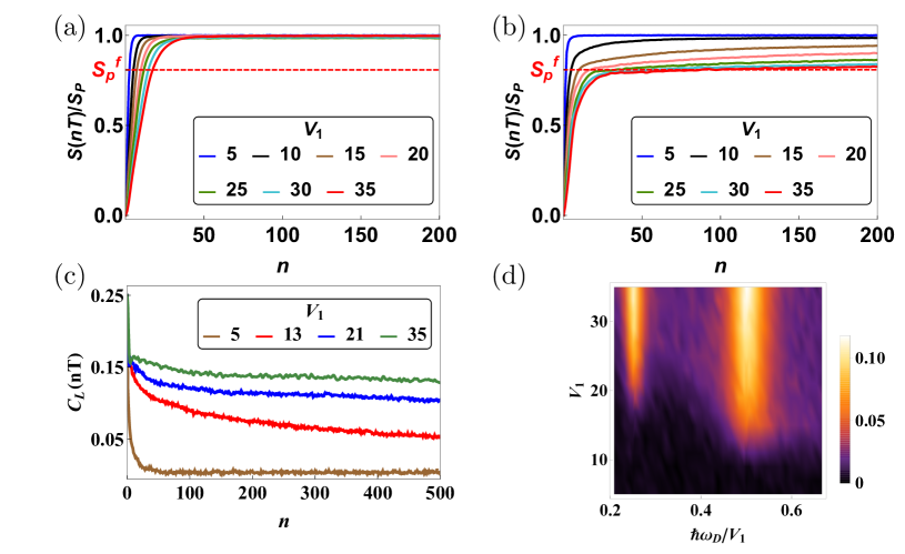
Figure 1: (Color Online) (a) Plot of $S(nT)/S_{p}$ as a function of $n$ at $\omega_{D}=V_{1}/\hbar$ starting from a random Fock state for different values of the drive amplitude $V_{1}$. For all values of $V_{1}$, $S(nT)$ saturates to $S_{p}$. (b) Similar to (a) but at the special frequency $\omega_{D}=V_{1}/2\hbar$. With increase in $V_{1}$, $S(nT)$ saturates to $S_{p}^{f}$, the Page value of the fragment of $H_{F}^{(1)}$ from which the initial Fock state is chosen, for $n\leq 200$. (c) Plot of the density-density autocorrelator $C_{L}(nT)$ as a function of $n$ at $\omega_{D}=V_{1}/2\hbar$ starting from a infinite temperature thermal state. In this case too, the autocorrelator does not reach its thermal value of zero within the first 500 drive cycles, thus bearing signatures of prethermal HSF. (d) Value of $C_{L}(nT)$ after $n=5000$ drive cycles as a function of $V_{1}$ and $\hbar\omega_{D}/V_{1}$. The plot shows two special frequencies at $\hbar\omega_{D}/V_{1}=0.25$ and $\hbar\omega_{D}/V_{1}=0.5$. The time evolutions are performed using the exact unitary evolution operators, corresponding to drive protocols (32) and (33). The system sizes are $L=16$ for plots (a) and (b) and $L=14$ for (c) and (d). For all plots, $J_{1}=J_{2}/3=0.5$ and $V_{0}=V_{2}=2$.

The derivation of the first order Floquet Hamiltonian from Eq. 41 and III.2 can be carried out in a straightforward manner [21] and yields

$$H_{F}^{(1)} = \hat{J}_{c}+V_{0}\sum_{j}\hat{n}_{j}\hat{n}_{j+1}+V_{2}\sum_{j}\hat{n}_{j}\hat{n}_{j+2}$$ (43)

Thus the fragmentation exhibited by $H_{F}^{(1)}$ for this protocol is identical to that found in Ref. 20. In addition, it also allows for variation of $J$ which makes the protocol much less restrictive compared to its counterpart in Ref. 20.

The corresponding dynamical signatures in the half-chain entanglement entropy and the density-density autocorrelation function are shown in Fig. 1. For these plots, we use Eqs. 32 and 33 and set the hopping amplitudes to $J_{1}=0.5$ for the first half of the drive and $J_{2}=1.5$ for the next half cycle in Fig. 1. Also, we set $V_{0}=V_{2}=2$. Figs. 1(a) and 1(b) show the evolution of the half-chain entanglement entropy starting from a random Fock state from the half-filled sector in a chain of length $L=16$ with periodic boundary condition at $\omega_{D}=V_{1}/\hbar$ (generic frequency) and $\omega_{D}=V_{1}/2\hbar$ (special frequency satisfying the relation in Eq. 42) respectively. Fig. 1(a) shows that away from the special frequency, for all values of the drive amplitude, the entanglement entropy $S(nT)$ saturates to the Page value $S_{p}$ of the half-filled symmetry sector from which the initial state is chosen, as is expected of ergodic systems. In contrast to this, Fig. 1(b) shows that at the special frequency, the entanglement entropy fails to reach $S_{p}$ with increasing drive amplitude within the first $200$ drive cycles. Instead, with increase in drive amplitude, $S(nT)$ saturates to $S_{p}^{f}$, the Page value of the fragment of $H_{F}^{(1)}$, from which the initial state is chosen. Both $S_{p}$ and $S_{p}^{f}$ have been computed analytically and numerically following Ref. 20.

Fig. 1(c) shows similar behavior for the time evolution of the density-density autocorrelator

$$C_{L}(nT)=\langle(n_{L}(nT)-1/2)(n_{L}(0)-1/2)\rangle$$ (44)

in an infinite temperature thermal state for a chain of length $L=14$ with open boundary condition at the special frequency $\omega_{D}=V_{1}/2\hbar$. A careful look at Eq. 44 reveals that $C_{L}$ also represents the connected autocorrelator since $\langle n_{L}(0)-1/2\rangle=0$. Thus, in an ergodic system, $C_{L}(nT)$ is expected to decay to zero at long enough times signifying loss of any initial memory. However, Fig. 1(c) shows that with increasing drive amplitude $V_{1}$, $C_{L}$ saturates to a value much higher than zero at long enough times. This can be explained by considering the fragmented structure of $H_{F}^{(1)}$ and the Mazur’s bound on the autocorrelator in the presence of the fragmented structure [20]. In [20], we had seen that the long-time saturation value of the autocorrelator was above the lower bound predicted by the Mazur’s bound. The autocorrelator decays down to zero when the chain is driven away from the special frequencies. Fig. 1(d) elucidates this by plotting the value of $C_{L}(nT)$ after $5000$ drive cycles as a function of the drive amplitude and the drive frequency. This plot can also serve as a “phase diagram” in the drive frequency and drive amplitude space, where non-zero saturation values of $C_{L}(nT)$ (bright regions in the color plot) indicate parameter regimes where prethermal fragmentation is observed.

It is to be noted here that for a given drive amplitude, the rate of thermalization is faster as compared to that reported in [20]. This is to be attributed to the asymmetric drive protocol (different values of the hopping amplitude during the two half-cycles) used here. Due to the asymmetric nature of the protocol, the lowest non-trivial correction to the constrained Hamiltonian at the special frequency comes from the second-order Floquet Hamiltonian, $H_{F}^{(2)}$ as compared to $H_{F}^{(3)}$ in [20]. This, in turn, results in a shorter thermalization timescale.

IV Other filling fractions

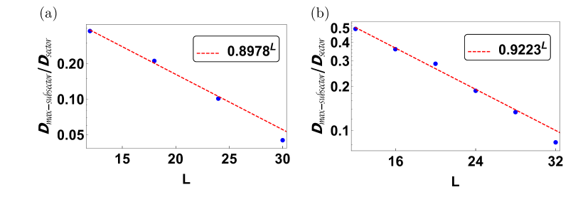
Figure 2: (Color Online) (a) Plot of the ${\mathcal{D}}_{\rm sub-sector}/{\mathcal{D}}_{\rm sector}$ for $H_{F}^{(1)}$ as a function of $L$ for $N/L=1/3$ showing exponential reduction with $L$ similar to the half-filling case. (b) Similar plot for $N/L=1/4$. For both plots, $J=1$ and $V_{1}/(\hbar\omega_{D})=2m$.

In this section, we study the driven fermion chain away from half-filling to demonstrate the robustness of the fragmentation signature. To this end, we consider the driven fermion chain at filling fractions $N/L=1/3,1/4$ (where $N$ is the fermion number and $L$ is the chain length). In what follows, we shall use the square-pulse protocol given by $V(t)=-(+)V_{1}$ for $t\leq(>)T/2$ in accordance with Ref. 20.

We begin our study by analyzing the Hilbert space dimension (HSD) of the largest fragment of the first order Floquet Hamiltonian (Eq. 13) at $N/L=1/3$ and $1/4$. This is shown in Fig. 2 where the ratio of the HSD of the largest fragment, ${\mathcal{D}}_{{\rm sub-sector}}$, and the total HSD of the symmetry sector (one-third filled sector in (a) and one-fourth filled sector in (b)), ${\mathcal{D}}_{{\rm sector}}$, is plotted as a function of $L$ for $J=1$ and at a special frequency $V_{1}/(\hbar\omega_{D})=2m$, where $m$ is an integer. We find a clear signature of exponential decay of this ratio for both $1/3$ and $1/4$ filling fractions as a function of $L$. This indicates the possibility of the presence of signature of strong HSF in the dynamics of the driven chain at these filling.

To verify this expectation, we compute the entanglement entropy $S(nT)$ as a function of $n$ and at different drive frequencies. For an ergodic driven system, $S$ is expected to increase with $n$ and eventually saturate to its Page value corresponding to the symmetry sector $S_{p}$ irrespective of the initial state chosen for the dynamics[27]. In contrast, for a chain which exhibits HSF, $S(nT)$ is expected to saturate to the Page value of the fragment to which the initial state belongs: $S\to S_{p}^{f}$. Thus the saturation value of $S$ is lower; also it depends on the initial state from which the dynamics originates. This allows one to distinguish between dynamical behavior of a driven chain with and without strong HSF. A plot of $S(nT)/S_{p}$, shown in Fig. 3(a) for $N/L=1/3$ and Fig. 3(b) for $N/L=1/4$, clearly shows the distinction between the behavior of $S$ at and away from the special frequencies. $S(nT)/S_{p}$ saturates, for both fillings, to unity at large $n$ away from the special frequencies($V_{1}/(\hbar\omega_{D})=1/2$); in contrast, at the special frequency $V_{1}/(\hbar\omega_{D})=2$, they saturate to a lower value which corresponds to $S_{p}^{f}$ of the respective sectors from which the initial states are chosen.

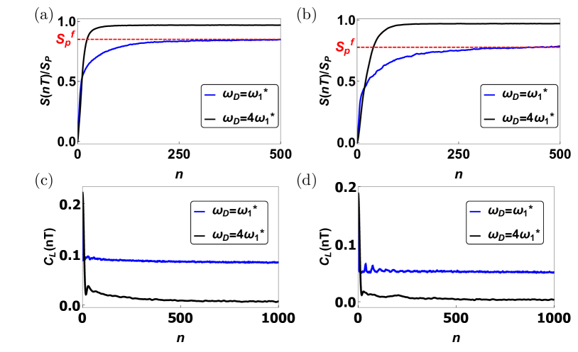
Figure 3: (Color Online) (a) Growth of entanglement entropy from exact dynamics for $L=18$ and $N=6$, starting from a randomly chosen Fock state. The result is averaged over 10 such states chosen from the same fragment of the first order Floquet Hamiltonian. The sector dimension from which the state is chosen is $1980$. The entanglement entropy is scaled by the Page value $S_{p}$ of the symmetry sector for which $N/L=1/3$. At the special frequencies, EE saturates to a value less than $S_{p}$ but close to $S_{p}^{f}$ for the fragment from which the initial state was chosen. (b) Same as in (a) but for $L=20$ and $N=5$ corresponding to $1/4$ filling. The sector dimension of the fragment from which the initial state is chosen is $1050$. (c) Plot of $C_{L}(nT)$ as a function of $n$ at the special frequency $V_{1}/(\hbar\omega_{d})=2$ and away from it $V_{1}/(\hbar\omega_{D})=1/2$ for $N/L=1/3$ and $L=18$ The initial state is same as in (a). (d) Same as (c) but for $L=20$ and $N/L=1/4$; the initial state is same as in (b). For all plots $J=1$.

In addition, we compute the density-density autocorrelation function given by Eq. 44. Fig. 3(c) and (d) show the behavior of $C_{L}(nT)$ as a function of $n$ at and away from the special frequency for $N/L=1/3$ and $1/4$ respectively. We find that in both cases, $C_{L}(nT)$ saturates to finite value at the special frequency and to zero away from it. Thus these plots confirm the existence of strong HSF similar to the half-filling sectors in these fermionic chains.

Finally, in Fig. 4, we show the plot of $S(nT)/S_{p}$ starting from several initial Fock states which belong to different sectors with different values of $S_{p}^{f}$ for $V_{1}/(\hbar\omega_{D})=2$. We find that in each case, both at $N/L=1/3$ (Fig. 4(a)) and $1/4$ (Fig. 4(b)), $S(nT)/S_{p}<1$ for large $n$; moreover, $S(nT)\to S_{p}^{f}$ corresponding to the fragment of $H_{F}^{(1)}$ to which the initial state belongs. This clearly demonstrates signature of HSF at these filling fractions.

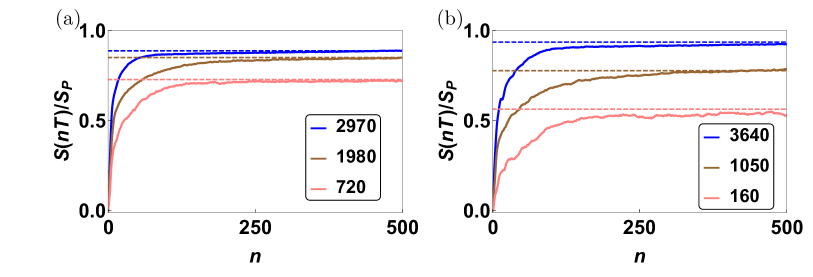
Figure 4: (Color Online) Plot of $S(nT)/S_{p}$ as a function of $n$ at $V_{1}/(\hbar\omega_{D})=2$ starting from Fock states belonging to different fragments for (a) $L=18$ and $N=6$ and (b) $L=20$ and $N=5$. The numbers label the Hilbert space dimensions of the fragments and the dashed lines indicate the corresponding $S_{p}^{f}$. For all plots $J=1$.

V Density-density out-of-time ordered correlation function

In this section we analyze the out-of-time ordered correlator (OTOC) for the driven chain. The basic definitions are outlined in Sec. V.1. This is followed by numerical study of OTOC for a chain with periodic boundary condition (PBC) and starting from an infinite temperature thermal state in Sec. V.2. Finally we study the behavior of OTOC for fermion chains with open boundary condition (OBC) and starting from the ${\mathbb{Z}}_{2}=|0,1,0,1,\ldots\rangle$ Fock state in Sec. V.3.

V.1 Preliminary

The study of OTOC serves as an important tool to diagnose the rate of propagation of local information in a quantum system [29, 30, 31, 32]. Ergodic systems are known to exhibit ballistic spread of local information accompanied by a diffusive front. In case of non-ergodic systems, the behavior of information propagation, as detected using OTOC, ranges from logarithmic growth in many-body localized systems [33] to alternate scrambling and unscrambling in certain integrable systems [34]. For fragmented systems, the scrambling of information is expected to be slow since the Hamiltonian does not connect states belonging to different fragments; however, its detailed features, in the presence of a periodic drive, have not been studied earlier.

To probe the rate of scrambling of information in our system, we study the temporal (in stroboscopic times) and spatial profile of the OTOC

$$F(r,nT) = \langle\tilde{n}_{i}(nT)\tilde{n}_{j}(0)\tilde{n}_{i}(nT)\tilde{n}_{j}(0)\rangle,$$ (45)

where $\tilde{n}_{i}=2n_{i}-1$ with $n_{i}$ and $n_{j}$ being the number density operators at sites $i$ and $j$ respectively and $r=|i-j|$ measures the distance between these two sites. We take the average with respect to both an infinite-temperature thermal state and the $|{\mathbb{Z}}_{2}\rangle$ state. Since the operator $\tilde{n}_{i}$ is hermitian and squares to identity, it can be shown that the function $F(r,nT)$ is related to the squared commutator $C(r,nT)$ as

$$C(r,nT) = \langle[\tilde{n}_{i}(nT),\tilde{n}_{j}]^{\dagger}[\tilde{n}_{i}(nT),\tilde{n}_{j}]\rangle$$ (46)

$$= 2(1-F(r,nT)).$$

Cast in this form, it can be argued that as the operator $\tilde{n}_{i}$, initially localized at site $i$, spreads to the site $j$, the value of $C(r,nT)$ at this site gradually increases from zero and hence the OTOC, $F(r,nT)$ decreases from $1$. A higher value of $C(r,nT)$ (i.e. lower value of $F(r,nT)$) at a given instant of time therefore indicates larger spread of the local operator ($\tilde{n}_{i}$ in the present case).

V.2 Infinite-temperature initial state

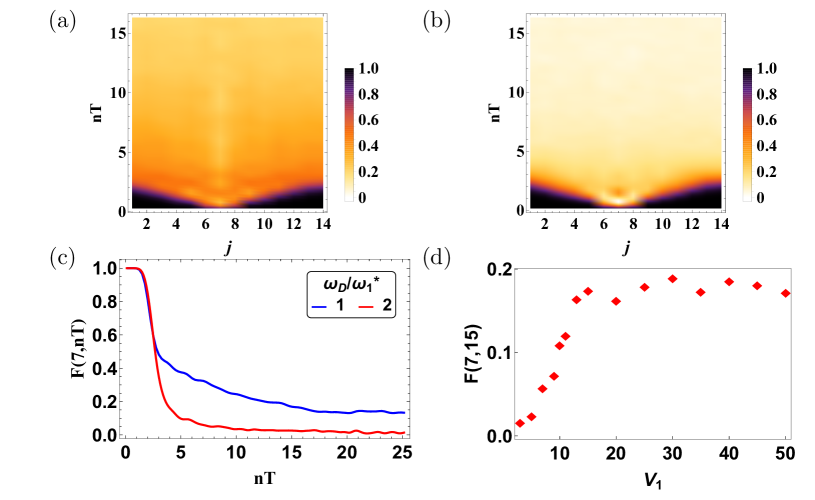
Figure 5: (Color Online) (a) Profile of the OTOC $F(r,nT)$ in an infinite temperature thermal state for $L=14$ (half-filled sector) with PBC and $\omega_{D}=V_{1}/\hbar$. The initial operator $\tilde{n}_{i}$ is localized at the centre of the chain $i=7$. The index $j$ in the x-axis labels the site of the chain and $r=|j-7|$ for all plots. A ballistic spread of information is seen with the value of the OTOC rapidly dropping close to zero as is expected of a thermalizing system. (b) Same as (a) but at the special frequency $\omega_{1}^{*}=V_{1}/2\hbar$, where the first-order Floquet Hamiltonian $H_{F}^{(1)}$ is fragmented. Although there is some information scrambling in this case due to mixing of states within fragments, the value to which $F(r,nT)$ reaches at similar times is higher as compared to the thermalizing case. This implies that the extent of information scrambling is less in this case, compared to (a). (c) Profile of $F(r,nT)$ at site $j=14$ both at and away from the special frequency $\omega_{1}^{*}$, illustrating the same point. (d) Variation of the value of $F(r,nT)$ at the farthest site $j=14$ after $t=nT=15$ with drive amplitude $V_{1}$ and $\omega_{D}=\omega_{1}^{\ast}$. With decrease in $V_{1}$, higher-order terms in the pertubation series gain prominence and enhance information scrambling. For all plots, $J=1,V_{0}=V_{2}=2$. For (a)-(c), $V_{1}=50$. All the results are obtained using the exact time-evolution operator.

In this section, we study the spread of OTOC in an infinite-temperature thermal state for a half-filled chain of length $L=14$ with PBC both at the special frequency ($\hbar\omega_{1}^{*}=V_{1}/2$, shown in Fig 5(b)) and away from it ($\omega_{D}=2\omega_{1}^{*}$, shown in Fig 5(a)). The operator is initially localized at the centre of the chain, i.e. $i=L/2$ in both the cases. Fig. 5(a) shows that at a generic frequency, the operator spreads ballistically. Such a spread can be inferred from the linear variation of $r$, for sites at which $F(r,t)$ has almost similar values, as a function of $t$.

$F(r,nT)$ quickly falls to a value close to zero, implying that $C(r,nT)$ saturates to a value close to $1$. At the special frequency, however, Fig. 5(b) shows that although the local information reaches the farthest site almost at the same time as in the previous case, the OTOC saturates to a higher value as compared to its thermalizing counterpart. This is a direct consequence of the fact that the first order Floquet Hamiltonian $H_{F}^{(1)}$, which is fragmented, only allows mixing of the states within a particular fragment. Although the infinite-temperature thermal initial state (represented by a density matrix) weighs all the states equally, during time evolution they can only be connected with states belonging to the same fragment. As a result, they fail to spread out through the whole Hilbert space. The information is scrambled only due to mixing between states within individual fragments; this leads to lower scrambling in the prethermal regime than that due to ergodic evolution away from the special frequency. Fig. 5(c) illustrates this fact by plotting the value of $F(r,nT)$ for site $j=14$ both at and away from the special frequency. As the drive amplitude decreases, the higher order terms in the perturbation series start dominating, allowing mixing between different fragments. This enhances information scrambling leading to a decrease in the value of the OTOC. This is shown in Fig. 5(d) which plots the variation of the value of OTOC at the farthest site ($j=14$) at $nT=15$ as a function of $V_{1}$ for $\omega_{D}=\omega_{1}^{\ast}$. This shows that information scrambling is suppressed beyond a critical $V_{1}$ where signatures of fragmentation can be found over a long pre-thermal timescale.

V.3 $\mathbb{Z}_{2}$ State

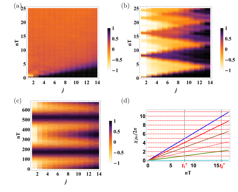
Figure 6: (Color Online) (a) Profile of the OTOC $F(r,nT)$ in a $\mathbb{Z}_{2}$ state for L=14 with OBC and at a generic frequency $\omega_{D}=V_{1}/\hbar$. The initial operator $\tilde{n}_{i}$ is localized at one of the edges of the chain $i=1$. The information reaches to the other end of the system ballistically, bearing signature of thermalizing systems. (b) Same as (a) but at the special frequency $\omega_{1}^{*}=V_{1}/2\hbar$. The information after reaching the other end starts unscrambling again. This alternate scrambling and unscrambling of information continues over a short timescale, dictated by the quasienergy spectrum of the fragmented $H_{F}^{(1)}$ as explained in the main text. (c) Long-time oscillations in the profile of the OTOC at $\omega_{1}^{*}$. (d) Plot of $\chi_{\beta\alpha}(nT)$ (defined below Eq. 51 in the main text) as a function of $t=nT$. The color codes are: $\chi_{28}$ (blue), $\chi_{38}$ (red), $\chi_{48}$ (brown), $\chi_{58}$ (pink), $\chi_{68}$ (green) and $\chi_{78}$ (cyan). The red dashed lines mark integer multiples of $2\pi$. The first two times when these phases are very close integer multiples of $2\pi$, are marked as $t_{1}^{*}$ and $t_{2}^{*}$ respectively. These correspond to the first two recurrence times in (b). For all plots, $J=1,V_{0}=V_{2}=2,V_{1}=50$.

In this section, we study the spatial and temporal profile of the OTOC in a $|{\mathbb{Z}}_{2}\rangle$ state at the special frequency with OBC. Fig. 6(a) shows that away from the special frequency, starting from one end of the chain, the information propagates ballistically to the other end, as is expected for a ergodic system; $F(r,t)$ monotonically decays to near-zero value at all sites within $nT\leq 10$. In contrast, as shown in Fig. 6(b) and (c), at the special frequency the behavior of $F(r,nT)$ is quite different and it shows signature of fragmentation. In Fig. 6(b), we find that at short time scales $nT\sim$ 10, there are initial fast oscillations which lead to alternate scrambling and unscrambling of information. Such alternate scrambling and unscrambling of information is reminiscent of the behavior of OTOC in integrable systems [34]; however, as we show below, the mechanism for this phenomenon is different in the present case. Furthermore, over longer time scales $nT\sim$ 100 - 500, we find slow oscillatory behavior as seen in Fig. 6(c). As discussed below, this is related to tunneling between two near degenerate states.

Both the above oscillatory features can be related to the fact that at high drive amplitude and at the special frequencies, the dynamics is mostly governed by $H_{F}^{(1)}$ at short and intermediate timescales. To understand the behavior of $F$, we therefore focus on the fragment of $H_{F}^{(1)}$ (with OBC) to which $|{\mathbb{Z}}_{2}\rangle$ belongs. For $L=14$, there are $8$ states in this fragment namely

$$\mathcal{H}= \{|{\mathbb{Z}}_{2}\rangle,|j_{h}=2\rangle,|j_{h}=4\rangle,|j_{h}=6\rangle,$$

$$|j_{h}=8\rangle,|j_{h}=10\rangle,|j_{h}=12\rangle,|\bar{\mathbb{Z}}_{2}\rangle\}$$ (47)

where $|\bar{\mathbb{Z}}_{2}\rangle=|1,0,1,0,\ldots\rangle,\text{ and }|j_{h}\rangle$ is a state with one hole-defect (where aa hole-defect implies two adjacent unoccupied sites) at position $j_{h}$ and zero particle defect (i.e. no two adjacent sites are occupied), viz $|j_{h}=2\rangle=|1,0,0,1,0,1,0,1,0,1,0,1,0,1\rangle$. Note, the constrained hopping introduces dynamics between these eight states, and $H_{F}^{(1)}$ in this subspace is equivalent to a nearest neigbor hopping model of a linear chain with eight sites and OBC. Here $|{\mathbb{Z}}_{2}\rangle$ and $|\bar{\mathbb{Z}}_{2}\rangle$ form the ends of the chain while $j_{h}=2,4,\ldots,12$ form the sites in between.

The OTOC at a site $j$ will have the structure

$$F(r_{1},nT)=\langle\mathbb{Z}_{2}|\tilde{n}_{1}(nT)\tilde{n}_{j}(0)\tilde{n}_{1}(nT)\tilde{n}_{j}(0)|\mathbb{Z}_{2}\rangle$$ (48)

where $r_{1}=|j-1|$. Inserting the complete set of states $|m\rangle$ from this fragment and noting that the operator $\tilde{n}$ is diagonal in the Fock basis, this expression reads

$$F(r_{1},nT)\approx\sum_{m}(-1)^{j}f^{j}_{m}|\langle m(nT)|\tilde{n}_{1}|\mathbb{Z}_{2}(nT)\rangle|^{2}$$ (49)

where $f^{j}_{m}=\langle m|\tilde{n}_{j}|m\rangle$. Expanding $|\mathbb{Z}_{2}\rangle$ and $|m\rangle$ in the energy eigenstates of $H_{F}^{(1)}$: $|\mathbb{Z}_{2}\rangle=\sum_{\alpha}c_{\alpha}|\phi_{\alpha}\rangle$, $|m\rangle=\sum_{\beta}c_{\beta}^{m}|\phi_{\beta}\rangle$, Eq. 49 yields

$$F(r_{1},nT)\approx\sum_{m}(-1)^{j}f^{j}_{m}g_{m}(nT)$$ (50)

where

$$g_{m}(nT)=\Big{|}\sum_{\alpha,\beta}c_{\beta}^{m*}c_{\alpha}e^{-i\chi_{\beta\alpha}(t)}N^{1}_{\beta\alpha}\Big{|}^{2}$$ (51)

with $N^{1}_{\beta\alpha}=\langle\phi_{\beta}|\tilde{n}_{1}|\phi_{\alpha}\rangle$ being the matrix element of $\tilde{n}_{1}$ between the energy eigenstates and $\chi_{\beta\alpha}(t)=(\epsilon_{\alpha}-\epsilon_{\beta})nT/\hbar$.

V.3.1 Short and Long time Oscillations

In Eq. 50 the spatial dependence on $r_{1}$ or $j$ is factorized out from the time dependence $nT$. This implies that the time dependence of the OTOC is site-independent, i.e. the recurrence time at every site is the same and the recurrence happens when all the phases $\chi_{\beta\alpha}(t)$ are approximately close to integer multiples of $2\pi$. We arrange the spectrum $\epsilon_{1}<\epsilon_{2}<\ldots<\epsilon_{8}$. Numerically, we find that the matrix elements $N^{1}_{\beta\alpha}$ between the states $|\phi_{\beta}\rangle;\beta=2,3,\ldots,8$ and $|\phi_{\alpha}\rangle;\alpha=7,8$ are an order of magnitude higher than the rest of the off-diagonal matrix elements. This is because the states $\beta=1,2,\ldots,6$ are mostly made of the six single-hole wavefunction, while the states $\alpha=7,8$ are mostly made of the states $\mathbb{Z}_{2}$ and $\bar{\mathbb{Z}}_{2}$. Since the last two states have one extra next-nearest-neighbor interaction compared to the first six, $\epsilon_{\alpha\beta}\sim V_{2}$, and this energy scale shows up in the fast oscillations seen over timescales $nT\sim$ 10. Thus, in this relatively short time, the recurrence is predominantly dictated by the phases $\chi_{\beta\alpha}(t)$ with $\beta=2,3,\ldots,7$ and $\alpha=8$. Fig. 6(d) plots these phases as a function of $t=nT$. It can be seen that the recurrence occurs when all these phases are close to $2\pi p_{0}$ (where $p_{0}\in Z$) as shown in Fig. 6(d). The first two of these times are marked with $t_{1}^{*}$ and $t_{2}^{*}$ in Fig.6(d). These are not exactly periodic because of involvement of multiple phases in the dynamics. It is also to be noted from Fig. 6(d) that the energies $\epsilon_{7,8}$ (which are mostly linear combinations of $\mathbb{Z}_{2}$ and $\bar{\mathbb{Z}}_{2}$ Fock states) are so close that for the short timescale involved, the phase $\chi_{87}(t)$ almost remains close to zero; it does not play much role in determining the short recurrence time. Thus, from the above discussion it is clear that the recurrences at short timescales owe their existence to two features in the model. First, the finite next-nearest-neighbor interaction energy $V_{2}$. Second, the OBC which allows the single-hole states to be included within the same fragment as to which the states $\mathbb{Z}_{2}$ and $\bar{\mathbb{Z}}_{2}$ belong (with PBC, the fragment has only the $\mathbb{Z}_{2}$ and $\bar{\mathbb{Z}}_{2}$ states).

In Fig. 7(a), we show the comparison between results for $F(r_{1},nT)$ obtained from exact dynamics (solid lines) and the analytical estimate obtained from $H_{F}^{(1)}$ in Eq. 50 (dashed lines) for some representative sites $j=1,5,14$. It can be seen that the first two recurrence times at $t_{1}^{*}=8.07,t_{2}^{*}=16.21$ are well approximated by Eq. 50.

The phase $\chi_{87}(t)$ manifests itself only at longer time scales of $nT\sim$ 100 - 500. As seen in Fig. 6(c), over this time scale $F(r_{1},nT)$ oscillates from values nearly one to nearly minus one with frequency $\Omega$, where $\Omega=(\epsilon_{8}-\epsilon_{7})/\hbar$. In Fig. 7(b) and (c) we show that these oscillations can be explained using Eq 50 by considering the $8$ states belonging to this fragment of $H_{F}^{(1)}$. In Appendix B, we show that a four state ansatz can be used to arrive at this result for a high next-nearest-neighbor interaction strength, when the $\mathbb{Z}_{2}$, $\bar{\mathbb{Z}}_{2}$ states are well separated in energy from the remaining $|j_{h}\rangle$ states.

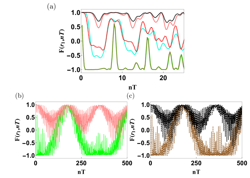
Figure 7: (Color Online) (a) Comparison of exact and approximate estimate (Eq. 50) of $F(r_{1},nT)$ for $j=1$ (green solid, brown dashed), $j=5$ (cyan solid, red dashed) and $j=14$ (pink solid, black dashed) sites. The solid lines represent results obtained from exact dynamics and dashed lines represent approximate estimates obtained using the fragment of $H_{F}^{(1)}$. The first two recurrence times are in good agreement, emphasizing the role of fragmentation in the scrambling and unscrambling behavior observed in Fig. 6(b). For $j=1$, the agreement between approximate and exact numerical result is nearly perfect and the green solid and the brown dashed lines are almost on top of each other. (b), (c) Similar comparison for the long time oscillations for $j=1,14$, following the color scheme used in (a). (b) Plot of exact numerical result for $j=1,14$. (c) Plot of approximate estimate for $j=1,14$.

V.3.2 Spatial profile of OTOC

The spatial dependence in the profile of the OTOC appears through the term $h_{jm}=(-1)^{j}f^{j}_{m}$ in Eq. 50. The initial linear increase in Fig. 6(b) for $nT\leq 5$ can be explained by focusing on this term. The profile of $h_{jm}$ for odd $j$’s reads

$$h_{jm}=\begin{pmatrix}1&-1&-1&-1&-1&-1&-1&-1\\ 1&1&-1&-1&-1&-1&-1&-1\\ 1&1&1&-1&-1&-1&-1&-1\\ 1&1&1&1&-1&-1&-1&-1\\ 1&1&1&1&1&-1&-1&-1\\ 1&1&1&1&1&1&-1&-1\\ 1&1&1&1&1&1&1&-1\\ \end{pmatrix}$$ (52)

where the rows label the odd sites $j=1,3,5,\ldots 13$ and the columns label the different Fock states $|m\rangle$ in this fragment, in the same order as in Eq. 47. The time dependent functions $g_{m}(nT)$ are positive definite at all times. As $j$ increases, the number of $g_{m}(nT)$’s having positive weights increases linearly as is evident from Eq. 52. Thus, the shift of $F(r_{1},nT)$ from $1$ happens progressively at a later time as $j$ increases. It is also useful to note that $f^{2k-1}_{m}=-f^{2k}_{m}$ for all $k\text{ and }m$, so that $h_{2k-1,m}=h_{2k,m}$ and hence at any given instant of time, $F(2k-1,nT)=F(2k-2,nT)$. Thus the even sites $j$ have similar behavior as the odd sites.

VI Discussion

In this work, we studied the dynamics of a periodically driven Fermi chain and extended the study of prethermal HSF in these system undertaken in Ref. 20 in several ways.

First, we have studied the existence of such prethermal HSF beyond half-filling in such chains. We found the existence of such prethermal HSF phase for several other filling fractions such as $N/L=1/4$ and $1/3$. This shows that the robustness of the pretheraml MBL phase in such driven chain.

Second, we provide a derivation of the first and second order Floquet Hamiltonian in such driven system in an alternative manner. Our derivation brings out the commutator structure of the Floquet Hamiltonian; in particular, we find that the second order term in the Floquet Hamiltonian, $H_{F}^{2}$, can be expressed as a commutator of a constrained current operator $\sum_{j}A_{j}(c_{j}^{\dagger}c_{j}-h.c.)$ with $H_{F}^{(1)}$. We expect similar commutation relations to hold for higher order terms in $H_{F}$; this sheds light on the symmetry content of the higher order terms in the Floquet Hamiltonian for the cosine drive protocol.

Third, we extend our analysis to experimentally relevant and slightly more complicated drive protocols. In a typical experiment, involving ultracold atoms, the interaction strength between fermions and their hopping strength are both controlled by intensities of the applied lasers. Consequently, experimentally relevant protocols must allow change of both the hopping amplitudes and interaction strength. We show that the prethermal HSF is stable for a large class of such drives and chart out a phase diagram for the special frequencies at which it occurs.

Finally, we study the behavior of density-density OTOC for such driven systems. Our study shows that such OTOCs can serve as detectors of such prethermal HSF in two distinct ways. First, irrespective of the boundary condition used, the OTOC $F(r,t)$ for a finite fermion chain driven at the special frequency and starting from a ${\mathbb{Z}}_{2}$ initial state, exhibits a larger long-time value than when driven away from such frequencies. In addition, it also exhibits oscillations with very large periodicity at the special frequencies that have the same origin as the correlation functions discussed in Ref. 20. In contrast, no such oscillations are found when one is away from the special frequency; the OTOC monotonically decreases to zero. Second, for fermion chains with open boundary condition and driven at special frequencies, we find periodic scrambling and unscrambling of information which is in sharp contrast to standard behavior of OTOCs in driven ergodic systems. Such a behavior was found earlier for integrable spin chains [34]; however, their origin for systems with prethermal HSF quite different and can be tied to the localization of the driven system within a group of Fock states with same dipole number ($n_{d}=0$). For chains with open boundary condition, there are $O(L)$ such states which govern the dynamics up to a long prethermal time scale leading to periodic scrambling and unscrambling. This phenomenon is qualitatively different from the behavior of OTOC away from the special frequencies where it monotonically decays due to fast spread of the driven system through the Hilbert space; it is also different for a chain with PBC with two Fock states (${\mathbb{Z}}_{2}$ and ${\bar{\mathbb{Z}}_{2}}$) in the $n_{d}=0$ sector where no such unscrambling is found.

Experimental verification of our result would require realization of isolated fermi chain. A possible scenario for this is a $1D$ fermion systems with nearest neighbor hopping and local interaction realized suing ultracold fermions in an optical lattice. We propose to drive this with the experimentally relevant protocol discussed in this work; this can be achieved by varying strength of lasers used to generate the lattice [24, 25]. The simplest measurement would involve measuring $\langle\hat{n}_{d}\rangle$ as a function of time. We predict that the dynamics of $\langle n_{d}\rangle$ staring from the ${\mathbb{Z}}_{2}$ state for such a chain will be approximately constant (and close to zero) for a long prethermal timescale when the system is driven at the special frequency. This is to be contrasted the behavior of $\langle n_{d}\rangle$ away from the special frequency which should exhibit rapid dynamics at short timescale.

In conclusion, we have studied several aspects of prethermal HSF in a driven Fermi chain. Our results have showed the robustness of this phenomenon by confirming its existence for different, experimentally relevant, drive protocols and also when the system is away from half-filling. In addition we have demonstrated that OTOCs may serve as a marker for such prethermal HSF; they exhibit periodic scrambling and unscrambling for fermion chains with open boundary condition driven at the special frequency.

Acknowledgement: SG acknowledges CSIR, India for support through project 09/080(1133)/2019-EMR-I. IP thanks Edouard Boulat for discussions. KS thanks DST, India for support through SERB project JCB/2021/000030 and Arnab Sen for discussions.

Appendix A Computation of $\mathcal{H}_{F}^{(2)}$ for cosine protocol

The second order Floquet Hamiltonian can be broken into two parts $\mathcal{H}_{F}^{(2)}=\mathcal{H}_{F}^{(2a)}+\mathcal{H}_{F}^{(2b)}$. From Eq. (26) we get

$$\mathcal{H}_{F}^{(2a)} =\frac{-iJ^{2}}{2\hbar T}\sum_{i,j}\sum_{m,n}B_{m,n}\left[J_{m}(\lambda\hat{A}_{i})c^{\dagger}_{i}c_{i+1}+J_{m}(-\lambda\hat{A}_{i})\right.$$

$$\times\left.c^{\dagger}_{i+1}c_{i}\,,\,J_{n}(\lambda\hat{A}_{j})c^{\dagger}_{j}c_{j+1}+J_{n}(-\lambda\hat{A}_{j})c^{\dagger}_{j+1}c_{j}\right],$$ (53)

where

$$B_{m,n}\equiv\int_{0}^{T}d\tau_{1}\int_{0}^{\tau_{1}}d\tau_{2}\,e^{im\omega\tau_{1}}e^{in\omega\tau_{2}}$$ (54)

The evaluation of the above integrals yield

$$B_{m,n} =\frac{T^{2}}{2}\delta_{m,0}\delta_{n,0}+\frac{T}{im\omega}\delta_{n,0}(1-\delta_{m,0})$$

$$-\frac{T}{in\omega}\delta_{m,0}(1-\delta_{n,0})+\frac{T}{in\omega}(1-\delta_{n,0})\delta_{m,-n}.$$ (55)

Due to the commutator structure of Eq. (A) the first and the fourth terms above do not contribute. The second and the third terms are non-zero and equal. Next, due to the $1/m$ factor in the second term, only integers $m$ contribute. We get

$$\mathcal{H}_{F}^{(2a)} =-\frac{2J^{2}}{\hbar\omega}\sum_{k=0}^{\infty}\frac{1}{2k+1}\left[\sum_{i}J_{2k+1}(\lambda\hat{A}_{i})\right.$$

$$\times\left.\left(c^{\dagger}_{i}c_{i+1}-{\rm h.c.}\right)\,,\,\sum_{j}J_{0}(\lambda\hat{A}_{j})\left(c^{\dagger}_{j}c_{j+1}+{\rm h.c.}\right)\right].$$ (56)

Noting that $\hat{A}_{i}$ can only take values 0, 1, -1, we have the relation

$$J_{2k+1}(\lambda\hat{A}_{i})=\hat{A}_{i}J_{2k+1}(\lambda).$$

Using the above we get

$$\mathcal{H}_{F}^{(2a)} =-\frac{2J^{2}}{\hbar\omega}\mathcal{C}(\lambda)\left[\sum_{i}\hat{A}_{i}\left(c^{\dagger}_{i}c_{i+1}-{\rm h.c.}\right)\right.\,,\,$$

$$\left.\sum_{j}J_{0}(\lambda\hat{A}_{j})\left(c^{\dagger}_{j}c_{j+1}+{\rm h.c.}\right)\right],$$ (57)

where

$$\mathcal{C}(\lambda)\equiv\sum_{k=0}^{\infty}\frac{J_{2k+1}(\lambda)}{2k+1}.$$

For the second term $\mathcal{H}_{F}^{(2b)}$ we note that

$$\int_{0}^{T}d\tau_{1}\int_{0}^{\tau_{1}}d\tau_{2}\tilde{\mathcal{H}}_{p}(\tau_{2})=\int_{0}^{T}d\tau_{1}\int_{\tau_{1}}^{T}d\tau_{2}\tilde{\mathcal{H}}_{p}(\tau_{1}).$$

Using the above relation and Eq. (III.1) we get

$$\mathcal{H}_{F}^{(2b)} =\frac{i}{2\hbar T}\int_{0}^{T}d\tau(T-2\tau)\left[\tilde{\mathcal{H}}_{p}(\tau)\,,\,\hat{K}\right]$$

$$=\frac{-iJ}{2\hbar T}\sum_{i,m}\int_{0}^{T}d\tau(T-2\tau)e^{im\omega\tau}$$

$$\times\left[J_{m}(\lambda\hat{A}_{i})c^{\dagger}_{i}c_{i+1}+J_{m}(-\lambda\hat{A}_{i})c^{\dagger}_{i+1}c_{i}\,,\,\hat{K}\right]$$

For the $\tau$-integral above we use the relation

$$\int_{0}^{T}d\tau(T-2\tau)e^{im\omega\tau}=-\frac{2T}{im\omega}(1-\delta_{m,0}).$$

The appearance of the factor $1/m$ in the above implies that, again, only the Bessel functions with odd indices contribute. This gives

$$\mathcal{H}_{F}^{(2b)}=\frac{2J\mathcal{C}(\lambda)}{\hbar\omega}\left[\sum_{i}\hat{A}_{i}\left(c^{\dagger}_{i}c_{i+1}-{\rm h.c.}\right)\,,\,\hat{K}\right].$$ (58)

The Eqs. (A) and (58) imply Eq. (30) in the main text.

Appendix B 4-state ansatz for the long-time OTOC oscillations

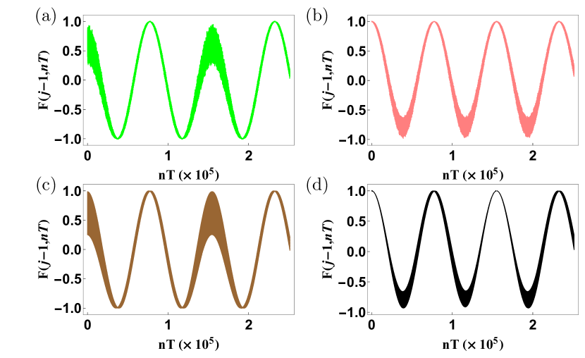
Figure 8: (Color Online) Comparison of exact results for OTOC $F(r_{1},nT)$ with that obtained from Eq. 61 and 63, starting from a $|\mathbb{Z}_{2}\rangle$ state. (a) Green (light-colored) line is obtained from exact dynamics for $j=1$, (b) Pink (light-colored) line is obtained from exact dynamics for $j=14$, (c) Brown (dark-colored) is obtained from the 4 state ansatz, given by Eq. 59 for $j=1$. (d)Black (dark-colored) is obtained from the 4 state ansatz, for $j=14$. For all the plots, $L=14,V_{0}=2,V_{2}=6$ and $V_{1}=50$ with $\omega_{D}=V_{1}/2\hbar$.

In this section, we discuss a simplification of Eq. 50 when a high value of the next-nearest-neighbor interaction $V_{2}$ is considered. In this case, the $\{|\mathbb{Z}_{2}\rangle,|\bar{\mathbb{Z}}_{2}\rangle\}$ states, which have one extra next-nearest-neighbor pair, are well separated in energy from the other $|j_{h}\rangle$ states. Thus, the extent of hybridization between $\{|\mathbb{Z}_{2}\rangle,|\bar{\mathbb{Z}}_{2}\rangle\}$ states and the $|j_{h}\rangle$ is small and hence the eigenfunctions of $H_{F}^{(1)}$ can be written down in terms of only a few Fock states as we show below.

We assume that the two highest energy levels $|\phi_{7}\rangle$ and $|\phi_{8}\rangle$ are mostly symmetric and anti-symmetric combinations of $\mathbb{Z}_{2}$ and $\bar{\mathbb{Z}}_{2}$ with very small contributions from the two “nearest” $|j_{h}\rangle$ states, i.e. $|j_{h}=2\rangle$ and $|j_{h}=12\rangle$. By “nearest”, we refer to states which can be connected to $\mathbb{Z}_{2},\bar{\mathbb{Z}}_{2}$ by one constrained hop. We also consider two more states $|\phi_{5,6}\rangle$ which are orthogonal to $|\phi_{7,8}\rangle$ and have energies $\epsilon_{5,6}$. We assume these last two states to be nearly degenerate i.e. $\epsilon_{5}\approx\epsilon_{6}=E_{0}$ and the splitting between the two highest states $\epsilon_{8}-\epsilon_{7}=\Omega\ll V_{2}$, $\epsilon_{7}-\epsilon_{6}=V_{2}$. Thus

$$|\phi_{8}\rangle = \frac{1}{\sqrt{2}}\mathcal{C}(|\mathbb{Z}_{2}\rangle-|\bar{\mathbb{Z}}_{2}\rangle)+\frac{1}{\sqrt{2}}\mathcal{S}(|2\rangle-|12\rangle)$$

$$|\phi_{7}\rangle = \frac{1}{\sqrt{2}}\mathcal{C}(|\mathbb{Z}_{2}\rangle+|\bar{\mathbb{Z}}_{2}\rangle)+\frac{1}{\sqrt{2}}\mathcal{S}(|2\rangle+|12\rangle)$$

$$|\phi_{6}\rangle = \frac{1}{\sqrt{2}}\mathcal{S}(|\mathbb{Z}_{2}\rangle-|\bar{\mathbb{Z}}_{2}\rangle)-\frac{1}{\sqrt{2}}\mathcal{C}(|2\rangle-|12\rangle)$$

$$|\phi_{5}\rangle = \frac{1}{\sqrt{2}}\mathcal{S}(|\mathbb{Z}_{2}\rangle+|\bar{\mathbb{Z}}_{2}\rangle)-\frac{1}{\sqrt{2}}\mathcal{C}(|2\rangle+|12\rangle)$$ (59)

where $\mathcal{C}=\cos{\theta}$ and $\mathcal{S}=\sin{\theta}$ with $\theta$ being a phenomenological parameter to be determined from diagonalization. Inverting these relations, the time evolved states read

$$|\mathbb{Z}_{2}(t)\rangle = \frac{1}{\sqrt{2}}\left[\mathcal{C}e^{-iV_{2}t}(|\phi_{7}\rangle+|\phi_{8}\rangle e^{-i\Omega t})\right.$$

$$\left.+\mathcal{S}(|\phi_{5}\rangle+|\phi_{6}\rangle)\right]$$

$$|\bar{\mathbb{Z}}_{2}(t)\rangle = \frac{1}{\sqrt{2}}\left[\mathcal{C}e^{-iV_{2}t}(|\phi_{7}\rangle\right.$$

$$\left.-|\phi_{8}\rangle e^{-i\Omega t})+\mathcal{S}(|\phi_{5}\rangle-|\phi_{6}\rangle)\right]$$

$$|2(t)\rangle = \frac{1}{\sqrt{2}}\left[\mathcal{S}e^{-iV_{2}t}(|\phi_{7}\rangle\right.$$

$$\left.+|\phi_{8}\rangle e^{-i\Omega t})-\mathcal{C}(|\phi_{5}\rangle+|\phi_{6}\rangle)\right]$$

$$|12(t)\rangle = \frac{1}{\sqrt{2}}\left[\mathcal{S}e^{-iV_{2}t}(|\phi_{7}\rangle\right.$$ (60)

$$\left.-|\phi_{8}\rangle e^{-i\Omega t})-\mathcal{C}(|\phi_{5}\rangle-|\phi_{6}\rangle)\right]$$

where we have set the reference energy $E_{0}=0$. Using these 4 states, Eq. 49 for sites $j=1,14$ can be simplified as

$$F(0,nT)=f_{1}(nT)-f_{2}(nT)$$

$$F(13,nT)=f_{1}(nT)+f_{2}(nT)$$ (61)

where

$$f_{1}(nT) = |\langle\mathbb{Z}_{2}(nT)|\tilde{n}_{1}|\mathbb{Z}_{2}(nT)\rangle|^{2}-|\langle\bar{\mathbb{Z}}_{2}(nT)|\tilde{n}_{1}|\mathbb{Z}_{2}(nT)\rangle|^{2}$$

$$f_{2}(nT) = |\langle 2(nT)|\tilde{n}_{1}|\mathbb{Z}_{2}(nT)\rangle|^{2}+|\langle 12(nT)|\tilde{n}_{1}|\mathbb{Z}_{2}(nT)\rangle|^{2}$$

Using the time-evolved states in Eq. 60, we obtain

$$f_{1}(t) = \mathcal{C}^{8}\cos{2\Omega t}-2\mathcal{C}^{6}\mathcal{S}^{2}\sin{\Omega t}\big{(}\sin{(V_{2}+\Omega)t}-\sin{V_{2}t}\big{)}+2\mathcal{C}^{4}\mathcal{S}^{4}\left[2\cos{\Omega t}-1+2\big{(}1-\cos{(V_{2}+\Omega)t}-\cos{V_{2}t}\big{)}^{2}\right]$$

$$- 4\mathcal{S}^{2}\mathcal{C}^{2}\left(\mathcal{S}^{4}+\mathcal{C}^{4}\cos{\Omega t}\right)\left(1-\cos{(V_{2}+\Omega)t}-\cos{V_{2}t}\right)+\mathcal{S}^{8}$$

$$f_{2}(t) = \mathcal{S}^{2}\mathcal{C}^{2}\left[\mathcal{S}^{4}\big{(}\cos{(V_{2}+\Omega)t}-\cos{V_{2}t}\big{)}^{2}+\left(\mathcal{C}^{2}\sin{\Omega t}+\mathcal{S}^{2}(\sin{(V_{2}+\Omega)t}-\sin{V_{2}t})\right)^{2}+\left(\sin{(V_{2}+\Omega)t}+\sin{V_{2}t}\right)^{2}\right]$$ (63)

$$+ \mathcal{S}^{2}\mathcal{C}^{2}\left[\mathcal{S}^{2}-\mathcal{C}^{2}\cos{\Omega t}+(2\mathcal{C}^{2}-1)\left(\cos{(V_{2}+\Omega)t}+\cos{V_{2}t}-1\right)\right]^{2}$$

For $V_{2}\gg J$, $\theta\ll 1$, we retain up to quadratic terms in $\theta$, yielding

$$F(0,t) = \left(1-4\theta^{2}\right)\cos{2\Omega t}+6\theta^{2}-2\theta^{2}\cos{\Omega t}$$

$$+ 4\theta^{2}\cos{V_{2}t}(\cos{\Omega t}-1)$$

$$F(13,t) = \left(1-4\theta^{2}\right)\cos{2\Omega t}-6\theta^{2}-6\theta^{2}\cos{\Omega t}$$ (64)

$$+ 4\theta^{2}\cos{V_{2}t}(3\cos{\Omega t}+1)$$

We compare in Fig. 8 the exact results and those obtained from Eq. 63 for sites $j=1$ and $j=14$ where we find good agreement between the two. The parameters chosen are $V_{0}=2,V_{2}=6,V_{1}=50$ and $\omega_{D}=V_{1}/2\hbar$.

Appendix C OTOC in $\mathbb{Z}_{2}$ state with PBC

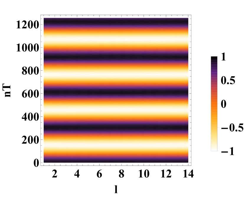
Figure 9: (Color Online) Profile of the OTOC $F(r,nT)$ in a $\mathbb{Z}_{2}$ state for $L=14$ with PBC and $\omega_{D}=V_{1}/2\hbar$. The initial operator is localized at $i=1$. This too shows alternate scrambling and unscrambling with a period $\tau\sim 300$. The parameters are $V_{0}=10V_{2}=2,V_{1}=20$

In this appendix, we consider the evolution of the profile of the OTOC starting from a $|\mathbb{Z}_{2}\rangle$ state with PBC at the special frequency. Fig. 9 shows that in this case too, there is alternate scrambling and unscrambling for $nT\leq 1200$ and $V_{0}=10V_{2}=2,V_{1}=20$. In the following we show that these oscillations can be interpreted as tunneling back and forth between the states $\mathbb{Z}_{2}$ and $\bar{\mathbb{Z}}_{2}$ when the system is close to the fragmented limit. Such tunneling events were reported in Ref. [20]. This can be understood by noting that for PBC, the $|\mathbb{Z}_{2}\rangle$ and $|\bar{\mathbb{Z}}_{2}\rangle$ states are degenerate frozen states for $H_{F}^{(1)}$. This degeneracy is lifted by higher-order hopping terms and for exact $H_{F}$, there are two eigenstates which are symmetric and anti-symmetric combinations of $|\mathbb{Z}_{2}\rangle$ and $|\bar{\mathbb{Z}}_{2}\rangle$ states viz

$$\chi_{+}=\frac{1}{\sqrt{2}}(|\mathbb{Z}_{2}\rangle+|\bar{\mathbb{Z}}_{2}\rangle),\quad\chi_{-}=\frac{1}{\sqrt{2}}(|\mathbb{Z}_{2}\rangle-|\bar{\mathbb{Z}}_{2}\rangle)$$

. The energy splitting between these two states is given by $\Omega=\epsilon_{-}-\epsilon_{+}$. This implies the time evolutions

$$|\mathbb{Z}_{2}(t)\rangle =e^{i\epsilon_{-}t}\left[(e^{i\Omega t}+1)|\mathbb{Z}_{2}\rangle+(e^{i\Omega t}-1)|\bar{\mathbb{Z}}_{2}\rangle\right]/2,$$

$$|\bar{\mathbb{Z}}_{2}(t)\rangle =e^{i\epsilon_{-}t}\left[(e^{i\Omega t}-1)|\mathbb{Z}_{2}\rangle+(e^{i\Omega t}+1)|\bar{\mathbb{Z}}_{2}\rangle\right]/2.$$ (65)

Inserting an approximate complete set comprising of the states $\mathbb{Z}_{2}$ and $\bar{\mathbb{Z}}_{2}$ in Eq. 48 of the main text, we obtain

$$F(r_{1},t)\approx\left|\langle\mathbb{Z}_{2}|\tilde{n}_{1}(t)|\mathbb{Z}_{2}\rangle\right|^{2}-\left|\langle\mathbb{Z}_{2}|\tilde{n}_{1}(t)|\bar{\mathbb{Z}}_{2}\rangle\right|^{2}$$

$$=\left|\langle\mathbb{Z}_{2}(t)|\tilde{n}_{1}|\mathbb{Z}_{2}(t)\rangle\right|^{2}-\left|\langle\mathbb{Z}_{2}(t)|\tilde{n}_{1}|\bar{\mathbb{Z}}_{2}(t)\rangle\right|^{2},$$ (66)

where the last line is going from Heisenberg to Schrodinger picture. Note, the above equation already captures an important aspect of Fig. 9, namely $F(r_{1},t)$ is mostly independent of $r_{1}$ at this timescale.

Using Eq. 65,we get

$$F(r_{1},t)\approx\cos(2\Omega t).$$ (67)

Thus, at stroboscopic times $t=nT$, where $n\Omega T$ is close to a integer multiple of $\pi$, the OTOC is close to one while, when $n\Omega T$ is close to a half-integer mutiple of $\pi$, the OTOC is close to minus one.

References

• [1] A. Polkovnikov, K., Sengupta, A. Silva, A. and M. Vengalattore, Rev. Mod. Phys. 83, 863 (2011).
• [2] L. D’Alessio, Y. Kafri, A. Polkovnikov, and M. Rigol, Adv. Phys. 65, 239 (2016).
• [3] M. Bukov, L. D’Alessio, and A. Polkovnikov, Adv. Phys. 64, 139 (2014).
• [4] J. M. Deutsch, Phys. Rev. A 43, 2046 (1991); M. Srednicki, Phys. Rev. E 50, 888 (1994); M. Srednicki, J. Phys. A 32, 1163 (1999).
• [5] M. Rigol, V. Dunjko, M. Olshanii, Nature 452, 854 (2008); P. Reimann, Phys. Rev. Lett. 101, 190403 (2008).
• [6] L. D’Alessio and M. Rigol, Phys. Rev. X 4, 041048 (2014).
• [7] M. Basko, I. L. Aleiner, and B. L. Altshuler, Ann. Phys. 321, 1126 (2006).
• [8] R. Nandkishore and D. Huse, Ann. Rev. Cond. Mat. 6, 15 (2015)
• [9] T. Kohlert, S. Scherg, X. Li, H. P. Luschen, S.D. Sarma, I. Bloch, and M. Aidelsburger, Phys. Rev. Lett. 122, 170403 (2019).
• [10] A. Chandran, T. Iadecola, V. Khemani, R. Moessner, Annual Review of Condensed Matter Physics 14, 443 (2023).
• [11] C. J. Turner, A. A. Michailidis, D. A. Abanin, M. Serbyn, and Z. Papi´c, Nat. Phys. 14, 745 (2018); S. Maudgalya, N. Regnault, and B. A. Bernevig, Phys. Rev. B 98, 235156 (2018).
• [12] W. W. Ho, S. Choi, H. Pitchler, and M. D. Lukin, Phys. Rev. Lett. 122, 040603 (2019); N. Shiraishi, J. Stat. Mech. 08313 (2019).
• [13] S. Choi, C. J. Turner, H. Pichler, W. W. Ho, A. A. Michailidis, Z. Papi´c, M. Serbyn, M. D. Lukin, and D. A. Abanin, Phys. Rev. Lett. 122, 220603 (2019); T. Iadecola, M. Schecter, and S. Xu, Phys. Rev. B 100, 184312 (2019).
• [14] P. A. McClarty, M. Haque, A. Sen and J. Richter, Phys. Rev. B 102, 224303(2020); D. Banerjee and A. Sen Phys. Rev. Lett. 126, 220601(2021); S. Biswas, D. Banerjee, and A. Sen, SciPost Phys. 12, 148 (2022).
• [15] V. Khemani, M. Hermele and R. Nandkishore, Phys. Rev. B 101, 174204 (2020); P. Sala, T. Rakovszky, R. Verresen, M. Knap and F. Pollmann, Phys. Rev. X 10, 011047 (2020).
• [16] T. Rakovszky, P. Sala, R. Verresen, M. Knap and F. Pollmann, Phys. Rev. B 101, 125126 (2020); Z.-C. Yang, F. Liu, A. V. Gorshkov and T. Iadecola, Phys. Rev. Lett. 124, 207602 (2020); G. De Tomasi, D. Hetterich, P. Sala, and F. Pollmann, Phys. Rev. B 100, 214313(2019); P. Frey, L. Hackl, and S. Rachel1, arXiv:2209.11777 (unublished); D. Vu, K. Huang, X. Li, and S. Das Sarma, Phys. Rev. Lett. 128, 146601 (2022).
• [17] S. Moudgalya and O. I. Motrunich, Phys. Rev. X 12, 011050 (2022); D. T. Stephen, O. Hart, and R. M. Nandkishore, arXiv:2209.03966 (unpublished); D. Hahn, P. A. McClarty, D. J. Luitz, SciPost Phys. 11, 074 (2021); N. Regnault and B. A. Bernevig, arXiv:2210.08019 (unpublished); T. Kohlert, S. Scherg, P. Sala, F. Pollmann, B. H. Madhusudhana, I. Bloch, and M. Aidelsburger, arXiv:2106.15586 (unpublished).
• [18] B. Mukherjee, D. Banerjee, K. Sengupta, and A. Sen, Phys. Rev. B 104, 155117 (2021); P. Brighi, M. Ljubotina, and M. Serbyn, arXiv:2210.15607 (unpublished).
• [19] A. Chattopadhyay, B. Mukherjee, K. Sengupta, and A. Sen, SciPost Phys. 14, 146 (2023); J Lehmann, P Sala, F Pollmann, and T Rakovszky, SciPost Phys. 14, 140 (2023); Y. H. Kwan, P. H. Wilhelm, S. Biswas, and S. A. Parameswaran, arXiv:2304.02669 (unpublished).
• [20] S. Ghosh, I. Paul, and K. Sengupta, Phys. Rev. Lett. 130, 120401 (2023).
• [21] A. Sen, D. Sen, and K. Sengupta, J. Phys. Condens. Matter 33, 443003 (2021).
• [22] A. Soori and D. Sen, Phys. Rev. B 82, 115432 (2010).
• [23] T. Bilitewski and N. R. Cooper, Phys. Rev. A 91, 063611 (2015).
• [24] I. Bloch, J. Dalibard, and W. Zwerger, Rev. Mod. Phys. 80, 885 (2008).
• [25] For a recent review, see J. Dobrzyniecki and T. Sowinski, Adv. Quantum Technol. 3, 2000010 (2020).
• [26] R. Ghosh, D. Das and K. Sengupta, JHEP 05, 172 (2021).
• [27] D. N. Page, Phys. Rev. Lett. 71, 1291 (1993); L. Vidmar and M. Rigol, Phys. Rev. Lett. 119, 220603 (2017).
• [28] P. Mazur, Physica 43, 533 (1969); J. Sirker, SciPost Phys. Lect. Notes 17, 1 (2020).
• [29] A. I. Larkin and Y. N. Ovichinnikov, Soviet J. Exp. Theor. Phys. 28, 1200 (1969); I. L. Aleiner, L. Faoro, and L. B. Ioffe, Ann. Phys-N. Y. 375, 378 (2016).
• [30] A. Nahum, S. Vijay, and J. Haah, Phys. Rev. X 8, 021014 (2018); C. W. von Keyserlingk, T. Rakovszky, F. Pollmann, and S. L. Sondhi, Phys. Rev. X 8, 021013 (2018); S. Xu, and B. Swingle, Locality, Phys. Rev. X 9, 031048 (2019).
• [31] M. Garttner, J. G. Bohnet, A. Safavi-Naini, M. L. Wall, J. J. Bollinger, and A. M. Rey, Nat. Phys. 13, 781 (2017).
• [32] For a recent review, see I. García-Mata, R. A. Jalabert, D. A. Wisniacki, Scholarpedia, 18, 55237 (2023)
• [33] Y. Chen, arXiv:1608.02765 (unpublished); R. Fan, P. Zhang, H. Shen, and H. Zhai, Science Bulletin 62, 707 (2017).
• [34] S. Sur and D. Sen, arXiv:2210.15302 (unpublished); ibid, arXiv:2310:12226 (unpublished).