Dynamic Conditional Optimal Transport through Simulation-Free Flows

Abstract

We study the geometry of conditional optimal transport (COT) and prove a dynamical formulation which generalizes the Benamou-Brenier Theorem. With these tools, we propose a simulation-free flow-based method for conditional generative modeling. Our method couples an arbitrary source distribution to a specified target distribution through a triangular COT plan. We build on the framework of flow matching to train a conditional generative model by approximating the geodesic path of measures induced by this COT plan. Our theory and methods are applicable in the infinite-dimensional setting, making them well suited for inverse problems. Empirically, we demonstrate our proposed method on two image-to-image translation tasks and an infinite-dimensional Bayesian inverse problem.

1 Introduction

Many fundamental tasks in machine learning and statistics may be posed as estimating or sampling from a distribution, where one only has access to the distribution via a finite set of observations. Such tasks range from generative modeling and density estimation to Bayesian inference. A broad range of methods for sampling from an intractable distribution $p$ may be seen through the lens of measure transport. Intuitively, one fixes a reference distribution $q$ which is easy to sample from, and samples $z\sim q$ are transformed by a learned mapping $T$ such that $T(z)$ is approximately distributed as $p$. The distribution obtained in this way from $q$, denoted $T_{\#}q$, is the pushforward of $q$ along $T$.

Generative models (Ho et al., 2020; Song et al., 2020; Kingma and Welling, 2013; Goodfellow et al., 2014; Papamakarios et al., 2021) typically find such a mapping $T$ by minimizing a divergence between the target and generated distribution. In the standard maximum-likelihood based setting, the mapping $T$ is learned by minimizing (an upper bound on) the KL divergence between $p$ and the pushforward $T_{\#}q$. However, a natural alternative approach, based on optimal transport (Villani et al., 2009; Santambrogio, 2015), is to search for a map $T$ which satisfies the constraint $T_{\#}q=p$ and has minimal cost (in some sense).

In many scenarios, we are interested in conditional sampling. That is, we have access to some observation $y\in Y$, and from this information we would like to infer information regarding an unknown quantity $u\in U$. For instance, in Bayesian inference, $y$ denotes the data and $u$ the parameters of a model. A joint distribution $p(y,u)=p(y\mid u)p(u)$ is specified via a likelihood $p(y\mid u)$ and a prior $p(u)$, and one would like to draw samples from the posterior $p(u\mid y)$. However, in applications such as Bayesian inverse problems (Dashti and Stuart, 2013), one is interested in approximating $p(u\mid y)$ for many different observations $y$. Moreover, in applications such as simulation-based inference (Cranmer et al., 2020), the likelihood function may be intractable while we are still able to sample from $p(y,u)$. This motivates an amortized and likelihood-free (Amos et al., 2023) approach, where a single model may be trained and applied across different observations.

In the framework of measure transport, we first specify a source distribution $q(u)$. For any given, fixed $y\in Y$, we seek to find a mapping $T(y)$, depending on $y$, such that $T(y)_{\#}q(u)\approx p(u\mid y)$. Finding such a mapping for each individual $y$ via optimal transport, though, is typically intractable, as we frequently do not have samples from the posterior $p(u\mid y)$. As such, we must leverage information from other observations. One way to achieve this is through triangular mappings (Baptista et al., 2020), where a joint source distribution $q(y,u)$ is transformed by a mapping of the form $T:(y,u)\mapsto(T_{Y}(y),T_{U}(y,u))$. It can be shown (see Section 3.2) that if $T_{\#}q=p$, then $T_{U}(y,{-})$ almost surely couples $q(u\mid y)$ and $p(u\mid y)$. Thus, if we are able to find such a triangular $T$ using samples from the joint distribution $p(y,u)$, then we may obtain conditional samplers.

In this work, we develop a dynamical framework for conditional optimal transport (COT). In particular, we study absolutely curves of measures in a conditional Wasserstein space over $Y\times U$. Our main results (Theorem 14 and Theorem 15) show that such curves are, informally stated, generated by the flow induced by a triangular vector field. Intuitively, a triangular vector field on $Y\times U$ has no velocity in the $Y$ component and thus induces a flow for each conditional measure. As a consequence, in Theorem 16 we obtain a conditional version of the well-known Benamou-Brenier theorem (Benamou and Brenier, 2000). Importantly, our framework is applicable in infinite-dimensional spaces, making it well suited for function space inference problems.

We apply our results on dynamical COT to design conditional generative models, based on the flow matching framework (Lipman et al., 2022; Albergo et al., 2023a) . In particular, we generalize the methods of Pooladian et al. (2023a) and Tong et al. (2023), which utilize optimal transport to pair source and target samples, to the conditional setting. Our method works by solving a relaxed optimal transport problem (Hosseini et al., 2023) during training. In this way, we amortize solutions to the dynamic COT problem across arbitrary $y$. Our method may use arbitrary source distributions, and is applicable across a wide range of conditional generative modeling tasks.

Specifically, the main contributions of our work are as follows.

1. In Section 4, we study the conditional Wasserstein space $\mathbb{P}_{p}^{\mu}(Y\times U)$ equipped with the conditional Wasserstein distance $W_{p}^{\mu}(Y\times U)$. We show that this space is a metric space, and moreover, admits constant speed geodesics between any two points.

2. In Section 5, we characterize the absolutely continuous curves of measures in $\mathbb{P}_{p}^{\mu}(Y\times U)$ via the continuity equation and triangular vector fields. As a corollary, we obtain a conditional version of the Benamou-Brenier theorem (Benamou and Brenier, 2000).

3. In Section 6 we propose a method for learning dynamic COT maps based on flow matching. In Section 7, we demonstrate our method on two image-to-image translation tasks, as well as an infinite-dimensional Bayesian inverse problem.

2 Related Work

Optimal Transport.

Machine learning based approaches to unconditional optimal transport plans typically focus on the static problem (Makkuva et al., 2020; Korotin et al., 2022; Taghvaei and Jalali, 2019). Approaches to learning optimal transport maps in a dynamic fashion often require restricted architectures (Bunne et al., 2022b) or use likelihood-based approaches (Tong et al., 2020; Finlay et al., 2020; Onken et al., 2021; Huguet et al., 2022), which require simulating from the model during training. While most work focuses on the squared norm cost, the recent approaches of Pooladian et al. (2023b) and Neklyudov et al. (2023) study dynamical optimal transport with costs specified by a Lagrangian. These frameworks, however, typically have no clear interpretation as a static problem.

Conditional optimal transport (COT), on the other hand, is relatively unexplored. Bunne et al. (2022a) and Wang et al. (2023) learn supervised COT maps in a static setting via convex networks (Makkuva et al., 2020). Hosseini et al. (2023) recently develop a framework for conditional optimal transport that is applicable in infinite-dimensional spaces. This builds on the work of Carlier et al. (2016) which applies COT for vector quantile regression. A common approach to COT is to employ triangular plans (Baptista et al., 2020). Our work develops a dynamic formulation of the static COT problem (Hosseini et al., 2023; Carlier et al., 2016) using a notion of triangular vector fields. Additionally, Wang et al. (2023) propose a likelihood-based approach using continuous normalizing flows, but do not develop the theory of dynamical COT as we do here.

Simulation-Free Continuous Normalizing Flows.

Flow matching (Lipman et al., 2022) and the equivalent stochastic interpolant framework (Albergo and Vanden-Eijnden, 2022; Albergo et al., 2023a) are a class of methods for building continuous-time normalizing flows in a simulation-free manner. These methods transform an arbitrary source distribution into a target distribution via a specified path of measures, which is modeled through a learned vector field. These methods have been extended to setting of Riemannian manifolds (Chen and Lipman, 2023) and infinite-dimensional spaces (Kerrigan et al., 2023).

Notably, these works do not approximate an optimal transport between the source and target measures and instead use an independent coupling, although stochastic interpolants (Albergo and Vanden-Eijnden, 2022; Albergo et al., 2023b) may be rectified (Liu et al., 2022; Lee et al., 2023) through an iterative optimization procedure. Importantly, the paths in flow matching (Lipman et al., 2022) maybe taken to be conditionally optimal, but marginally they are not. Pooladian et al. (2023a) and Tong et al. (2023) propose instead to couple the source and target distributions via optimal transport.

While some works (Lipman et al., 2022; Davtyan et al., 2023; Gebhard et al., 2023) have studied flow matching approaches for conditional distributions, these approaches simply provide additional conditioning information to the model and do not study COT. Concurrent work (Isobe et al., 2024) proposes extended flow matching, which learns a matrix field to perform conditional generation. However, the results of Isobe et al. (2024) are limited to the finite-dimensional setting and do not develop the theory of COT.

At the time of our submission, concurrent work by Barboni et al. (2024) and Chemseddine et al. (2024) appeared with similar results. Our results were developed independently from these works.

3 Background and Notation

Let $X,X^{\prime},X^{\prime\prime}$ represent arbitrary separable Hilbert spaces, equipped with the Borel $\sigma$-algebra. We use $\mathbb{P}(X)$ to represent the space of Borel probability measures on $X$, and $\mathbb{P}_{p}(X)\subseteq\mathbb{P}(X)$ to represent the subspace of measures having finite $p$th moment. If $\eta\in\mathbb{P}(X)$ is a probability measure on $X$ and $T:X\to X^{\prime}$ is measurable, then the pushforward measure $T_{\#}\eta({-})=\eta(T^{-1}({-}))$ is a probability measure on $X^{\prime}$. Maps of the form $\pi^{X}:X\times X^{\prime}\to X$ represent the canonical projection onto the respective space. We will also use maps such as $\pi^{1}:X\times X^{\prime}\times X^{\prime\prime}\to X$ and $\pi^{1,2}:X\times X^{\prime}\times X^{\prime\prime}\to X\times X^{\prime}$ to denote projection onto specific coordinates. The set $C_{b}(X)$ represents the space of continuous and bounded functions and $C^{\infty}_{c}(X)$ is the space of smooth and compactly supported functions.

In our specific case, we assume that we have two separable Hilbert spaces of interest. The first, $Y$, is a space of observations, and the second, $U$, is a space of unknowns. These spaces may be of infinite dimensions, but a special case of practical interest is when $Y$ and $U$ are finite dimensional Euclidean spaces. We will consider the product space $Y\times U$, equipped with the canonical inner product obtained via the sum of the inner products on $Y$ and $U$, under which the space $Y\times U$ is also a separable Hilbert space.

Let $\eta\in\mathbb{P}(Y\times U)$ be a joint measure. The measures $\pi^{Y}_{\#}\eta\in\mathbb{P}(Y)$ and $\pi^{U}_{\#}\eta\in\mathbb{P}(U)$ obtained via projection are the marginals of $\eta$. We use $\eta^{y}\in\mathbb{P}(U)$ to represent the measure obtained by conditioning $\eta$ on the value $y\in Y$. By the disintegration theorem, such conditional measures exist and are essentially unique, in the sense that there exists a Borel set $E\subseteq Y$ with $\pi^{Y}_{\#}\eta(E)=0$, and $\eta^{y}$ are unique for $y\notin E$.

3.1 Unconditional Optimal Transport

We provide here a brief overview of optimal transport in the standard unconditional setting. For more details, we refer to the standard references of Villani et al. (2009); Santambrogio (2015); Ambrosio et al. (2005). Fix a cost function $c:X\times X\to\mathbb{R}\cup\{+\infty\}$. Suppose we have two Borel measures $\eta,\nu\in\mathbb{P}(X)$. The Monge Problem seeks to find a measurable transport map $T:X\to X$ minimizing the expected cost of transport, i.e. corresponding to the optimization problem

$$\inf_{T}\left\{\int_{X}c(x,T(x))\,\mathrm{d}\eta(x)\mid T_{\#}\eta=\nu\right\}.$$ (1)

This optimization problem is challenging, though, as it involves a nonlinear constraint and the set of feasible maps may be empty. In contrast, the Kantorovich problem is a relaxation which seeks to find an optimal coupling $\gamma\in\Pi(\eta,\nu)$, i.e. a probability distribution over $X\times X$ with marginals $\eta,\nu$, which solves

$$\inf_{\gamma}\left\{\int_{X\times X}c(x_{0},x_{1})\,\mathrm{d}\gamma(x_{0},x_{1})\mid\gamma\in\Pi(\eta,\nu)\right\}.$$ (2)

Under fairly weak conditions (e.g., the cost is lower semicontinuous and bounded from below (Ambrosio et al., 2013, Theorem 2.5)), minimizers to the Kantorovich problem are guaranteed to exist. If the cost function is $c(x_{0},x_{1})=|x_{0}-x_{1}|^{p}$ for some $1<p<\infty$, under sufficient regularity conditions on $\eta$ a solution $T^{\star}$ to the Monge problem is guaranteed to exist and, moreover, the coupling $\gamma^{\star}=(I,T^{\star})_{\#}\eta$ is optimal for the Kantorovich problem. See Ambrosio et al. (2013, Chapter 2) and Ambrosio et al. (2005, Theorem 6.2.10).

Wasserstein Space.

In the special case that $c(x_{0},x_{1})=|x_{0}-x_{1}|^{p}$ for $1\leq p<\infty$, and $\eta,\nu\in\mathbb{P}_{p}(X)$, the Kantorovich problem admits a finite-cost solution. The cost of such an optimal coupling is the $p$-Wasserstein distance

$$W_{p}^{p}(\eta,\nu)=\min_{\gamma}\left\{\int_{X\times X}|x_{0}-x_{1}|^{p}\,\mathrm{d}\gamma(x_{0},x_{1})\mid\gamma\in\Pi(\eta,\nu)\right\}$$ (3)

which, as the name suggests, is a metric on the space $\mathbb{P}_{p}(X)$ (Ambrosio et al., 2005, Section 7.1) (Santambrogio, 2015, Section 5.1). The Wasserstein distance admits a dynamical formulation via the Benamou-Brenier theorem (Benamou and Brenier, 2000). Namely, the $p$-Wasserstein distance can be obtained by finding a time-dependent vector field transforming $\eta$ to $\nu$ across time $t\in[0,1]$ with minimal energy:

$$W_{p}(\eta,\nu)=\min_{(\gamma_{t},v_{t})}\left\{\int_{0}^{1}\int_{X}|v_{t}(x)|^{p}\,\mathrm{d}\gamma_{t}(x)\,\mathrm{d}t\mid\gamma_{0}=\eta,\gamma_{1}=\nu,\partial_{t}\gamma_{t}+\text{div}(v_{t}\gamma_{t})=0\right\}.$$ (4)

Here, we constrain our minimization problem over the set of measures and vector fields $(\gamma_{t},v_{t})$ interpolating between $\eta$ and $\nu$, satisfying a continuity equation (see Section 5.1). In Section 4, we study a generalization of the Wasserstein distances for conditional optimal transport problems. In particular, Theorem 16 provides a generalization of the Benamou-Brenier theorem to the conditional setting which recovers a conditional Wasserstein distance.

3.2 Static Conditional Optimal Transport

In the unconditional setting, one seeks an optimal coupling between two given measures. In contrast, in the conditional setting, we would like to find a family of couplings that can transport a given source measure into any conditional measure of the target distribution. In other words, given a target measure $\nu\in\mathbb{P}(Y\times U)$ and some source measure $\eta\in\mathbb{P}(U)$, one seeks a transport map $T:Y\times U\to U$ such that

$$T_{\#}(y,{-})_{\#}\eta=\nu^{y}\qquad\forall y\in Y.$$ (5)

If such a map were available, by drawing samples $u_{0}\sim\eta$ and transforming them, one would obtain samples $T(y,u)\sim\nu^{y}$. Solving this transport problem for each fixed $y$ is expensive at best, or impossible when only has a single (or no) samples $(y,u)\sim\nu$ for any given $y$.

Thus, one must leverage information across different observations $y$. To that end, recent work has focused on the notion of triangular mappings $T:Y\times U\to Y\times U$ (Hosseini et al., 2023; Baptista et al., 2020) (Bogachev and Ruas, 2007, Section 10.10) of the form

$$T(y,u)=\left(T_{Y}(y),T_{U}(T_{Y}(y),u)\right)$$ (6)

for some $T_{Y}:Y\to Y$ and $T_{U}:Y\times U\to U$. Triangular mappings are of interest as they allow us to obtain conditional couplings from joint couplings.

Proposition 1 (Theorem 2.4 (Baptista et al., 2020), Prop. 2.3 (Hosseini et al., 2023)).

Suppose $\eta,\nu\in\mathbb{P}(Y\times U)$ and $T:Y\times U\to Y\times U$ is triangular. If $T_{\#}\eta=\nu$, then $T_{U}(T_{Y}(y),{-})_{\#}\eta^{y}=\nu^{T_{Y}(y)}$ for $\pi^{Y}_{\#}\eta$-almost every $y$.

In many scenarios of practical interest, the source measure $\eta$ and the target measure $\nu$ have the same $Y$-marginals. We will henceforth make this assumption, and use $\mu=\pi^{Y}_{\#}\eta=\pi^{Y}_{\#}\nu$ to represent this marginal. In this case, we may take $T_{Y}$ to be the identity mapping, so that the conclusion of Proposition 1 simplifies to $T_{U}(y,{-})_{\#}\eta^{y}=\nu^{y}$ for $\mu$-almost every $y$. We note that in situations where such an assumption does not hold, one may simply preprocess the source measure $\eta$ via an invertible mapping $T_{Y}$ satisfying $[T_{Y}]_{\#}[\pi^{Y}_{\#}\eta]=\pi^{Y}_{\#}\nu$ (Hosseini et al., 2023, Prop 3.2).

Definition 2 (Conditional Wasserstein Space).

Suppose $\mu\in\mathbb{P}(Y)$ is a given probability measure over $Y$ and $1\leq p<\infty$. The set

$$\mathbb{P}^{\mu}(Y\times U)=\left\{\gamma\in\mathbb{P}_{p}(Y\times U)\mid\pi^{Y}_{\#}\gamma=\mu\right\}$$ (7)

is the space of joint measures on $Y\times U$ having fixed $Y$-marginals $\mu$. The set $\mathbb{P}_{p}^{\mu}(Y\times U):=\mathbb{P}^{\mu}(Y\times U)\cap\mathbb{P}_{p}(Y\times U)$ is the conditional $p$-Wasserstein space, consisting of joint measures with finite $p$th moments and $Y$-marginals $\mu$.

Given a source and target measures $\eta,\nu\in\mathbb{P}^{\mu}(Y\times U)$, the conditional Monge problem seeks to find a triangular mapping solving

$$\inf_{T}\left\{\int_{Y\times U}c(y,u,T(y,u))\,\mathrm{d}\eta(y,u)\mid T_{\#}\eta=\nu,T:(y,u)\mapsto(y,T_{U}(y,u))\right\}.$$ (8)

The conditional Monge problem also admits a relaxation under which one only considers couplings whose $Y$-components are almost surely equal. To that end, we consider the subset $\mathscr{C}\subset(Y\times U)^{2}$ whose $Y$ components are identical, i.e.,

$$\mathscr{C}:=\left\{(y_{0},u_{0},y_{1},u_{1})\in(Y\times U)^{2}\mid y_{0}=y_{1}\right\}$$ (9)

and we define the set of $(Y)$-restricted probability measures $\mathcal{R}_{Y}\subset\mathbb{P}\left((Y\times U)^{2}\right)$ such that every $\gamma\in\mathcal{R}_{Y}$ is concentrated on $\mathscr{C}$. In other words, if $\gamma\in\mathcal{R}_{Y}$, then samples $(y_{0},u_{0},y_{1},u_{1})\sim\gamma$ have $y_{0}=y_{1}$ almost surely. In addition, for any $\eta,\nu\in\mathbb{P}(Y\times U)$, we define the set of $(Y)$-restricted couplings $\Pi_{Y}(\eta,\nu)$ to be the probability measures in $\mathcal{R}_{Y}$ whose marginals are $\eta$ and $\nu$, i.e.

$$\Pi_{Y}(\eta,\nu)=\left\{\gamma\in\mathcal{R}_{Y}\mid\pi^{1,2}_{\#}\gamma=\eta,\pi^{3,4}_{\#}\gamma=\nu\right\}.$$ (10)

The conditional Kantorovich problem seeks a triangular coupling $\gamma^{\star}$ solving

$$\inf_{\gamma}\left\{\int_{(Y\times U)^{2}}c(y_{0},u_{0},y_{1},u_{1})\,\mathrm{d}\gamma(y_{0},u_{0},y_{1},u_{1})\mid\gamma\in\Pi_{Y}(\eta,\nu)\right\}.$$ (11)

Hosseini et al. (2023) prove the existence of minimizers to the conditional Kantorovich and Monge problems under very general assumptions. Moreover, optimal couplings to the conditional Kantorovich problem induce optimal couplings for $\mu$-almost every conditional measure. Assuming sufficient regularity assumptions on the conditional measures, unique solutions to the conditional Monge problem exist.

Proposition 3 (Prop 3.3 (Hosseini et al., 2023)).

Fix $\eta,\nu\in\mathbb{P}^{\mu}(Y\times U)$. Suppose the cost function $c$ is continuous, $\inf c>-\infty$, and there exists a finite cost coupling $\gamma\in\Pi_{Y}(\eta,\nu)$. Then, the conditional Kantorovich problem admits a minimizer $\gamma^{\star}$. Moreover, $\gamma^{\star,y_{0}}(y_{1},u_{0},u_{1})=\hat{\gamma}^{\star,y_{0}}(u_{0},u_{1})\delta(y_{1}-y_{0})$ where for $\mu$-almost every $y$ the measure $\gamma^{\star,y}$ is an optimal coupling for $\eta^{y},\nu^{y}$ under the cost $c^{y}(u_{0},u_{1})=c(y,u_{0},y,u_{1})$

Proposition 4 (Prop 3.8 (Hosseini et al., 2023)).

Fix $1<p<\infty$ and $\eta,\nu\in\mathbb{P}_{p}^{\mu}(Y\times U)$. Suppose $c(y_{0},u_{0},y_{1},u_{1})=|u_{0}-u_{1}|^{p}$. If $\eta^{y}$ assign zero measure to Gaussian null sets for $\mu$-almost every $y$, then there is a unique solution $T^{\star}$ to the conditional Monge problem, and $\gamma^{\star}=(I,T^{\star})_{\#}\eta$ is the unique solution to the conditional Kantorovich problem. If $\nu^{y}$ also assign zero measure to Gaussian null sets for $\mu$-almost every $y$, then $T^{\star}$ is injective $\eta$-almost everywhere.

4 Conditional Wasserstein Space

We now introduce a metric on the space $\mathbb{P}_{p}^{\mu}(Y\times U)$. Intuitively, the conditional Wasserstein distance measures the usual Wasserstein distance between all of the conditional distributions in expectation under the fixed $Y$-marginal $\mu$.

Definition 5 (Conditional $p$-Wasserstein Distance).

Suppose $\eta,\nu\in\mathbb{P}_{p}^{\mu}(Y\times U)$ and $1\leq p<\infty$. The function

$$W_{p}^{\mu}(\eta,\nu)=\left(\mathbb{E}_{y\sim\mu}\left[W_{p}^{p}(\eta^{y},\nu^{y})\right]\right)^{1/p}=\left(\int_{Y}W_{p}^{p}(\eta^{y},\nu^{y})\,\mathrm{d}\mu(y)\right)^{1/p}$$ (12)

is the conditional $p$-Wasserstein distance. Here, $W_{p}^{p}:\mathbb{P}_{p}(U)\times\mathbb{P}_{p}(U)\to\mathbb{R}$ is the usual $p$-Wasserstein distance for measures on $U$.

By an application of Jensen’s inequality we observe that $W_{p}^{\mu}(\eta,\nu)\geq\mathbb{E}_{y\sim\mu}\left[W_{p}(\eta^{y},\nu^{y})\right]$. For $p>1$, this inequality is strict unless $W_{p}(\eta^{y},\nu^{y})$ is $\mu$-almost surely constant. We emphasize that Definition 5 is purely formal at this stage. We do not know if this integral is well-defined, or if it actually defines a metric. Before proceeding, we first note that $W_{p}^{\mu}(\eta,\nu)$ may be viewed as the minimal value of the constrained Kantorovich problem in Equation (11) when one takes the cost to be the metric on the space $Y\times U$. Although Hosseini et al. (2023) studied the existence of minimizers to this problem, they did not study the metric properties of the resulting space.

Proposition 6 (Equivalent Formulation of the $p$-Wasserstein Distance).

Fix $\eta,\nu\in\mathbb{P}_{p}^{\mu}(Y\times U)$ and $1\leq p<\infty$. Then, $W_{p}^{\mu}(\eta,\nu)$ is well-defined, finite, and

$$W_{p}^{\mu,p}(\eta,\nu)=\min_{\gamma}\left\{\int_{(Y\times U)^{2}}d^{p}(y_{0},u_{0},y_{1},u_{1})\,\mathrm{d}\gamma\mid\gamma\in\Pi_{Y}(\eta,\nu)\right\}$$ (13)

where $W_{p}^{\mu,p}(\eta,\nu)$ represents the $p$-th power of the conditional $p$-Wasserstein distance.

Proof.

The cost function $d^{p}$ is clearly continuous and non-negative, and hence by Proposition 3 it suffices to exhibit a finite-cost coupling $\gamma\in\Pi_{Y}(\eta,\nu)$ between $\eta$ and $\nu$. Indeed, take the conditionally independent coupling

$$\gamma(y_{0},u_{0},y_{1},u_{1})=\eta(u_{0}\mid y_{1})\nu(u_{1}\mid y_{1})\delta(y_{1}-y_{0})\mu(y_{1})$$ (14)

which is clearly in $\Pi_{Y}(\eta,\nu)$. We then have that

$$\int_{(Y\times U)^{2}}d^{p}(y_{0},u_{0},y_{1},u_{1})\,\mathrm{d}\gamma(y_{0},u_{0},y_{1},u_{1})=\int_{(Y\times U)^{2}}\left\lVert(y_{0},u_{0})-(y_{1},u_{1})\right\rVert_{Y\times U}^{p}\,\mathrm{d}\gamma(y_{0},u_{0},y_{1},u_{1})$$

$$\leq 2^{p}\int_{(Y\times U)^{2}}\left(\left\lVert(y_{0},u_{0})\right\rVert_{Y\times U}^{p}+\left\lVert(y_{1},u_{1})\right\rVert_{Y\times U}^{p}\right)\,\mathrm{d}\gamma(y_{0},u_{0},y_{1},u_{1})$$

$$=2^{p}\left(\int_{Y\times U}\left\lVert(y_{0},u_{0})\right\rVert_{Y\times U}^{p}\,\mathrm{d}\eta(y_{0},u_{0})+\int_{Y\times U}\left\lVert(y_{1},u_{1})\right\rVert_{Y\times U}^{p}\,\mathrm{d}\nu(y_{1},u_{1})\right)<+\infty.$$

Hence, Equation (13) admits a minimizer $\gamma^{\star}\in\Pi_{Y}(\eta,\nu)$. By Proposition 3, this minimizer may be taken to have the form $\gamma^{\star}=\gamma^{\star,{y_{1}}}(u_{0},u_{1})\delta(y_{1}-y_{0})\mu(y_{1})$ where $\gamma^{\star,{y_{1}}}(u_{0},u_{1})$ is $\mu(y_{1})$-almost surely an optimal coupling between $\eta^{y_{1}},\nu^{{y_{1}}}$ for the cost $|u_{1}-u_{0}|^{p}$. Thus,

$$\int_{(Y\times U)^{2}}d^{p}\,\mathrm{d}\gamma^{\star} =\int_{Y}\int_{U^{2}}|u_{1}-u_{0}|^{p}\,\mathrm{d}\gamma^{\star,y}(u_{0},u_{1})\,\mathrm{d}\mu(y)$$ (15)

$$=\int_{Y}W_{p}^{p}(\eta^{y},\nu^{y})\,\mathrm{d}\mu(y)=W_{p}^{p,\mu}(\eta,\nu).$$ (16)

Here, we emphasize that the $\mu$-almost sure uniqueness of the disintegrations of $\eta,\nu$ along $Y$ result in a well-defined expression.

Moreover, if $\eta\in\mathbb{P}_{p}^{\mu}(Y\times U)$ it follows that $\eta^{y}\in\mathbb{P}_{p}(U)$ for $\mu$-a.e. $y$, because

$$\int_{Y}\int_{U}|u|^{p}\,\mathrm{d}\eta^{y}(u)\,\mathrm{d}\mu(y) \leq\int_{Y}\int_{U}|(y,u)|^{p}\,\mathrm{d}\eta^{y}(u)\,\mathrm{d}\mu(y)$$ (17)

$$=\int_{Y\times U}|(y,u)|^{p}\,\mathrm{d}\eta(y,u)<+\infty.$$ (18)

Thus all considered $p$-Wasserstein distances on $U$ are finite. ∎

We now show that $W_{p}^{\mu}$ is a metric on $\mathbb{P}_{p}^{\mu}(Y\times U)$.

Proposition 7 ($W_{p}^{\mu}$ is a Metric).

For $1\leq p<\infty$, the conditional $p$-Wasserstein distance $W_{p}^{\mu}$ is a metric on $\mathbb{P}_{p}^{\mu}(Y\times U)$.

Proof.

Fix $\eta,\nu,\rho\in\mathbb{P}_{p}^{\mu}(Y\times U)$. Since $W_{p}$ is a metric on $\mathbb{P}_{p}(U)$, we immediately obtain the symmetry of $W_{p}^{\mu}$. Moreover, we have that $W_{p}^{\mu}(\eta,\nu)=0$ if and only if $\eta^{y}=\nu^{y}$ for $\mu$-almost every $y$. Thus, if $W_{p}^{\mu}(\eta,\nu)=0$ and $E\subseteq Y\times U$ is Borel measurable,

$$\eta(E)=\int_{Y}\eta^{y}(E^{y})\,\mathrm{d}\mu(y)=\int_{Y}\nu^{y}(E^{y})\,\mathrm{d}\mu(y)=\nu(E).$$ (19)

which shows that $\eta=\nu$. Here, $E^{y}=\{u\mid(y,u)\in E\}$ is the $y$-slice of $E$. Conversely, if $\eta=\nu$, then $\eta^{y}=\nu^{y}$ up to a $\mu$-null set by the essential uniqueness of disintegrations. Thus, $W_{p}^{\mu}(\eta,\nu)=0$ if and only if $\eta=\nu$.

By Minkowski’s inequality and the triangle inequality for $W_{p}$ on $\mathbb{P}_{p}(U)$, we see

$$W_{p}^{\mu}(\eta,\nu) \leq\left(\mathbb{E}_{y\sim\mu}\left[(W_{p}(\eta^{y},\rho^{y})+W_{p}(\rho^{y},\nu^{y}))^{p}\right]\right)^{1/p}$$ (20)

$$\leq\mathbb{E}_{y\sim\mu}[W_{p}^{p}(\eta^{y},\rho^{y})]^{1/p}+\mathbb{E}_{y\sim\mu}[W_{p}^{p}(\rho^{y},\nu^{y})]^{1/p}$$ (21)

$$=W_{p}^{\mu}(\eta,\rho)+W_{p}^{\mu}(\rho,\nu).$$ (22)

∎

4.1 Metric Properties of Conditional Wasserstein Distances

We now briefly explore some properties of the space $\mathbb{P}_{p}^{\mu}(Y\times U)$ equipped with the conditional Wasserstein distance $W_{p}^{\mu}$. In particular, we observe that the topology on $\mathbb{P}_{p}^{\mu}(Y\times U)$ generated by $W_{p}^{\mu}$ is stronger than that generated by $W_{p}$. Note that we easily see $W_{p}^{\mu}(\eta,\nu)\geq W_{p}(\eta,\nu)$ for every $\eta,\nu\in\mathbb{P}_{p}^{\mu}(Y\times U)$ by the characterization in Proposition 6. The converse is, however, false, and the metrics are inequivalent.

Proposition 8 ($W_{p}^{\mu}$ is stronger than $W_{p}$).

There does not in general exist a constant $C>0$ such that $W_{p}^{\mu}(\eta,\nu)\leq CW_{p}(\eta,\nu)$ for all $\eta,\nu\in\mathbb{P}_{p}^{\mu}(Y\times U)$.

Proof.

We provide a counterexample. Fix any $u_{0}\neq 0\in U$ and $y_{0},y_{1}\in Y$ such that $y_{0}\neq y_{1}$. Define $\mu=\frac{1}{2}\left(\delta_{y_{0}}+\delta_{y_{1}}\right)$. Set $u_{k}=(k+1)u_{0}$ for $k=1,2,\dots$ and for each $k$, define two measures on $Y\times U$ by

$$\eta_{k}=\frac{1}{2}\left(\delta_{y_{0}u_{0}}+\delta_{y_{1}u_{k}}\right)\qquad\nu_{k}=\frac{1}{2}\left(\delta_{y_{1}u_{0}}+\delta_{u_{k}y_{0}}\right).$$ (23)

It is clear that

$$W_{p}^{\mu,p}(\eta_{k},\nu_{k})=k^{p}|u_{0}|^{p}\qquad W_{p}^{p}(\eta_{k},\nu_{k})=\min\{k^{p}|u_{0}|^{p},|y_{1}-y_{0}|^{p}\}.$$ (24)

Moreover, as $k\to\infty$ we have $W_{p}^{\mu}(\mu_{k},\nu_{k})\to\infty$ but $W_{p}^{p}(\nu_{k},\eta_{k})$ remains bounded. ∎

In addition, we can show that the conditional Wasserstein distance dominates the Wasserstein distance on the $U$ marginals.

Proposition 9 (Conditional Wasserstein Dominates $U$-Marginal Distance).

For $1\leq p<\infty$ and $\eta,\nu\in\mathbb{P}_{p}^{\mu}(Y\times U)$, we have

$$W_{p}\left(\pi^{U}_{\#}\eta,\pi^{U}_{\#}\nu\right)\leq W_{p}^{\mu}(\eta,\nu).$$ (25)

Proof.

Let $\gamma^{\star}(y_{0},u_{0},y_{1},u_{1})=\gamma^{\star,y_{1}}(u_{0},u_{1})\delta(y_{1}-y_{0})\mu(y_{1})$ be an optimal $\gamma^{\star}\in\Pi_{Y}(\eta,\nu)$. We claim that $\gamma(u_{0},u_{1}):=\int_{Y}\gamma^{\star,y}(u_{0},u_{1})\,\mathrm{d}\mu(y)$ couples $\pi^{U}_{\#}\eta$ and $\pi^{U}_{\#}\nu$. Let $\pi^{0}:(u_{0},u_{1})\mapsto u_{0}$ be the projection onto the first coordinate of $U\times U$. Observe that for $\mu$-almost every $y$, we have that $\gamma^{\star,y}\in\Pi(\eta^{y},\nu^{y})$ is optimal, and, in particular, $\pi^{0}_{\#}\gamma^{\star,y}=\eta^{y}.$ Fix an arbitrary $\varphi\in C_{b}(U)$. We then have

$$\int_{U}\varphi(u_{0})\,\mathrm{d}\pi^{0}_{\#}\gamma(u_{0})=\int_{U^{2}}(\varphi\circ\pi^{0})\,\mathrm{d}\gamma(u_{0},u_{1})$$ (26)

$$=\int_{Y}\int_{U^{2}}(\varphi\circ\pi^{0})\,\mathrm{d}\gamma^{\star,y}(u_{0},u_{1})\,\mathrm{d}\mu(y)=\int_{Y}\int_{U}\varphi(u_{0})\,\mathrm{d}\pi^{0}_{\#}\gamma^{\star,y}(u_{0})\,\mathrm{d}\mu(y)$$ (27)

$$=\int_{Y}\int_{U}\varphi(u_{0})\,\mathrm{d}\eta^{y}(u_{0})\,\mathrm{d}\mu(y){=}\int_{Y\times U}\varphi(u_{0})\,\mathrm{d}\eta(u_{0},y)$$ (28)

$$=\int_{Y\times U}(\varphi\circ\pi^{U})\,\mathrm{d}\eta(u_{0},y)=\int_{U}\varphi\,\mathrm{d}\pi^{U}_{\#}\eta(u_{0}).$$ (29)

Thus $\pi^{U}_{\#}\gamma=\pi^{U}_{\#}\eta$. A similar argument shows that for the map $\pi^{1}:(u_{0},u_{1})\mapsto u_{1}$ we have $\pi^{1}_{\#}\gamma=\pi^{U}_{\#}\nu$, so that $\gamma\in\Pi(\pi^{U}_{\#}\eta,\pi^{U}_{\#}\nu)$.

Now, as $\gamma^{\star,y_{1}}(u_{0},u_{1})\in\Pi(\eta^{y_{1}},\nu^{y_{1}})$ is $\mu$-almost surely optimal in the usual Wasserstein sense,

$$W_{p}^{p,\mu}(\eta,\nu) =\int_{Y}\int_{U^{2}}|u_{0}-u_{1}|^{p}\,\mathrm{d}\gamma^{\star,y}(u_{0},u_{1})\,\mathrm{d}\mu(y)$$ (30)

$$=\int_{U^{2}}|u_{0}-u_{1}|^{p}\,\mathrm{d}\gamma(u_{0},u_{1})$$ (31)

$$\geq W_{p}^{p}(\pi^{U}_{\#}\eta,\pi^{U}_{\#}\nu)$$ (32)

since $\gamma\in\Pi(\pi^{U}_{\#}\eta,\pi^{U}_{\#}\nu)$ is a coupling but potentially sub-optimal. ∎

Example: Gaussian Measures.

We conclude with an example where the conditional $2$-Wasserstein distance may be explicitly computed. In particular, this example shows that the inequality in Proposition 9 may be strict. Suppose $Y$ and $U$ are Euclidean spaces (of possibly different dimensions), and that $\eta,\nu\in\mathbb{P}_{p}^{\mu}(Y\times U)$ are Gaussians of the form

$$\eta=\mathcal{N}\left(\begin{bmatrix}m\\ m_{u}^{\eta}\end{bmatrix},\begin{bmatrix}\Sigma&\Sigma^{\eta}_{12}\\ \Sigma^{\eta}_{21}&\Sigma^{\eta}_{22}\end{bmatrix}\right)\qquad\nu=\mathcal{N}\left(\begin{bmatrix}m\\ m_{u}^{\nu}\end{bmatrix},\begin{bmatrix}\Sigma&\Sigma^{\nu}_{12}\\ \Sigma^{\nu}_{21}&\Sigma^{\nu}_{22}\end{bmatrix}\right).$$ (33)

It follows that $\mu=\pi^{Y}_{\#}\eta=\pi^{Y}_{\#}\nu=\mathcal{N}(m,\Sigma)$. Because we may obtain $\eta^{y},\nu^{y}$ in closed form, we can compute $W_{p}^{\mu}(\eta,\nu)$ in closed form. Let

$$Q^{\eta}=\Sigma_{22}^{\eta}-\Sigma_{21}^{\eta}\Sigma^{-1}\Sigma_{12}^{\eta}\qquad Q^{\nu}=\Sigma_{22}^{\nu}-\Sigma_{21}^{\nu}\Sigma^{-1}\Sigma_{12}^{\nu}\qquad R=(\Sigma_{21}^{\eta}-\Sigma_{21}^{\nu})\Sigma^{-1}$$ (34)

Then, we obtain by a brute-force calculation that

$$W_{2}^{\mu,2}(\eta,\nu)=|m_{u}^{\eta}-m_{u}^{\nu}|^{2}+\text{Tr}\left(Q^{\eta}+Q^{\nu}-2\left((Q^{\eta})^{1/2}Q^{\nu}(Q^{\eta})^{1/2}\right)^{1/2}+R\Sigma R^{T}\right).$$ (35)

Note that when $\eta,\nu$ have uncorrelated $Y,U$ components, we precisely recover $W_{2}^{2}(\pi^{U}_{\#}\eta,\pi^{U}_{\#}\nu)$ as one may expect. As a special case of interest, if $Y=U=\mathbb{R}$ and

$$\eta=\mathcal{N}(0,I)\qquad\nu=\mathcal{N}\left(0,\begin{bmatrix}1&\rho\\ \rho&1\end{bmatrix}\right)\quad|\rho|<1$$ (36)

then we obtain as a special case of Equation (35) that $W_{2}^{\mu,2}(\eta,\nu)=2(1-\sqrt{1-\rho^{2}})$. This is zero if and only if $\rho=0$, i.e. $\eta=\nu$. However, $\pi^{U}_{\#}\eta=\pi^{U}_{\#}\nu=\mathcal{N}(0,1)$.

4.2 Conditional Wasserstein Space as a Geodesic Space

In this section, we show that $\mathbb{P}_{p}^{\mu}(Y\times U)$ is a geodesic space. In fact, we show the stronger statement that there exists a constant speed geodesic between any two measures in $\mathbb{P}_{p}^{\mu}(Y\times U)$, which is a generalization of known results (Santambrogio, 2015, Theorem 5.27). First, we introduce some preliminary notions. A curve is a continuous function $\gamma_{\bullet}:I\to\mathbb{P}_{p}^{\mu}(Y\times U)$ where $I=(a,b)\subseteq\mathbb{R}$ is any open interval of finite length. A curve is said to be absolutely continuous if there exists $m\in L^{1}((a,b))$ such that

$$W_{p}^{\mu}(\gamma_{s},\gamma_{t})\leq\int_{s}^{t}m(\tau)\,\mathrm{d}\tau\qquad\forall a<s\leq t<b.$$ (37)

If $(\gamma_{t})$ is an absolutely continuous curve, then its metric derivative

$$|\gamma^{\prime}|(t)=\lim_{s\to t}\frac{W_{p}^{\mu}(\gamma_{s},\gamma_{t})}{|s-t|}$$ (38)

exists for almost every $t\in(a,b)$, and, moreover, we almost surely have $|\gamma^{\prime}|(t)\leq m(t)$ pointwise for any $m$ satisfying Equation (37) (Ambrosio et al., 2005, Theorem 1.1.2). A curve $(\gamma_{t})$ is called a constant speed geodesic if for all $a<s\leq t<b$, we have

$$W_{p}^{\mu}(\gamma_{s},\gamma_{t})=|t-s|W_{p}^{\mu}(\gamma_{a},\gamma_{b}).$$ (39)

It is straightforward to show that every constant speed geodesic is absolutely continuous.

Theorem 10 ($\mathbb{P}_{p}^{\mu}(Y\times U$) is a Geodesic Space).

$\mathbb{P}_{p}^{\mu}(Y\times U)$ admits constant-speed geodesics. That is, for any $\eta,\nu\in\mathbb{P}_{p}^{\mu}(Y\times U)$, there exists a constant speed geodesic, contained within $\mathbb{P}_{p}^{\mu}(Y\times U)$, between $\eta$ and $\nu$.

Proof.

Write $\lambda_{t}:(Y\times U)^{2}\to Y\times U$ for the linear interpolant

$$\lambda_{t}(y_{0},u_{0},y_{1},u_{1})=(ty_{0}+(1-t)y_{1},tu_{0}+(1-t)u_{1})\qquad 0\leq t\leq 1.$$ (40)

Let $\gamma^{\star}\in\Pi_{Y}(\eta,\nu)$ be an optimal restricted coupling, and consider the path of measures in $\mathbb{P}_{p}(Y\times U)$ given by

$$\gamma_{t}=[\lambda_{t}]_{\#}\gamma^{\star}\qquad 0\leq t\leq 1.$$ (41)

Step one: We check that for each $0\leq t\leq 1$, we have $\gamma_{t}\in\mathbb{P}_{p}^{\mu}(Y\times U)$. That is, we need to check that for all Borel $A\subseteq Y$, we have $\gamma_{t}(A\times U)=\mu(A)$. Indeed, recall that restricted measures are concentrated on the set $\mathscr{C}$ (see Equation (9)). Thus,

$$\gamma_{t}(A\times U) =\gamma^{\star}\left\{\lambda_{t}^{-1}(A\times U)\right\}$$

$$=\gamma^{\star}\left\{(y,u_{0},y,u_{1})\mid y\in A\right\}$$

$$=\pi^{1}_{\#}\gamma^{\star}(A)=(\pi^{1}\circ\pi^{1,2})_{\#}\gamma^{\star}(A)$$

$$=\pi^{1}_{\#}\eta(A)=\mu(A)$$

i.e. $\gamma_{t}(A\times Y)=\mu(A)$ as claimed.

Step two: We show that $W_{p}^{\mu}(\gamma_{t},\gamma_{s})=|t-s|W_{p}^{\mu}(\eta,\nu)$. Set $\gamma_{t}^{s}:=(\lambda_{t},\lambda_{s})_{\#}\gamma^{\star}$ for $0\leq s<t\leq 1$. We claim $\gamma_{t}^{s}\in\Pi_{Y}(\gamma_{t},\gamma_{s})$. Indeed, we have $\pi^{1,2}_{\#}\gamma_{t}^{s}=\gamma_{t}$ because for all Borel $A\subseteq Y\times U$,

$$(\lambda_{t},\lambda_{s})_{\#}\gamma^{\star}\left(A\times Y\times U\right)=\gamma^{\star}\left(\lambda_{t}^{-1}(A)\right)=(\lambda_{t})_{\#}\gamma^{*}(A).$$ (42)

An analogous calculation shows that $\pi_{\#}^{3,4}\gamma_{t}^{s}=\gamma_{s}$, so that $\gamma_{t}^{s}\in\Pi(\gamma_{t},\gamma_{s})$. We now check that $\gamma_{t}^{s}\in\mathcal{R}_{Y}(Y\times U)$. Indeed, suppose $E\subseteq Y\times U$ is a Borel set such that $E\cap\mathscr{C}=\varnothing$. In other words, for every $(y_{0},u_{0},y_{1},u_{1})\in E$ we have $y_{0}\neq y_{1}$. Set $D:=(\lambda_{t},\lambda_{s})^{-1}(E)$. We claim $D\cap\mathscr{C}=\varnothing$, so that

$$\gamma_{t}^{s}(E)=(\lambda_{t},\lambda_{s})_{\#}\gamma^{\star}(E) =\gamma^{\star}((\lambda_{t},\lambda_{s})^{-1}(E))$$ (43)

$$=\gamma^{\star}(D\cap\mathscr{C})=0.$$ (44)

Indeed, if $c=(y,u_{0},y,u_{1})\in\mathscr{C}$, then

$$(\lambda_{t},\lambda_{s})(c)=(y,tu_{0}+(1-t)u_{1},y,su_{0}+(1-s)u_{1})\notin E$$ (45)

$$\implies c\notin(\pi_{t},\pi_{s})^{-1}(E).$$ (46)

Thus $\gamma_{t}^{s}\in\Pi_{Y}(\eta,\nu)$ as claimed. Now, we have

$$W_{p}^{\mu,p}(\gamma_{t},\gamma_{s}) \leq\int_{(Y\times U)^{2}}d^{p}\left(y_{0},u_{0},y_{1},u_{1}\right)\,\mathrm{d}\lambda_{t}^{s}(y_{0},u_{0},y_{1},u_{1})$$

$$=\int_{(Y\times U)^{2}}d^{p}\left(\lambda_{t}(y_{0},u_{0},y_{1},u_{1}),\lambda_{s}(y_{0},u_{0},y_{1},u_{1})\right)\,\mathrm{d}\gamma^{\star}(y_{0},u_{0},y_{1},u_{1})$$

$$=\int_{(Y\times U)^{2}}\left(|(t-s)(y_{0}-y_{1})|^{2}+|(t-s)(u_{0}-u_{1})|^{2}\right)^{p/2}\,\mathrm{d}\gamma^{\star}(y_{0},u_{0},y_{1},u_{1})$$

$$=|t-s|^{p}\int_{(Y\times U)^{2}}d^{p}(y_{0},u_{0},y_{1},u_{1})\,\mathrm{d}\gamma^{\star}(y_{0},u_{0},y_{1},u_{1})$$

$$=|t-s|^{p}W_{p}^{\mu,p}(\eta,\nu).$$

Conversely, an application of the previous inequality and the triangle inequality show that for $0\leq s\leq t\leq 1$,

$$W_{p}^{\mu}(\eta,\nu) \leq W_{p}^{\mu}(\eta,\gamma_{s})+W_{p}^{\mu}(\gamma_{s},\gamma_{t})+W_{p}^{\mu}(\gamma_{t},\nu)$$ (47)

$$\leq sW_{p}^{\mu}(\eta,\nu)+W_{p}^{\mu}(\gamma_{s},\gamma_{t})+(1-t)W_{p}^{\mu}(\eta,\nu).$$ (48)

Rearranging the previous inequality implies $|t-s|W_{p}^{\mu}(\eta,\nu)\leq W_{p}^{\mu}(\gamma_{s},\gamma_{t})$ for all $s,t\in[0,1]$, and hence ${W_{p}^{\mu}(\gamma_{t},\gamma_{s})=|t-s|^{p}W_{p}^{\mu}(\eta,\nu)}$. ∎

When an optimal restricted coupling $\gamma^{\star}\in\Pi_{Y}(\eta,\nu)$ is induced by an injective triangular map $T^{\star}$, we may recover a constant speed geodesic in $\mathbb{P}_{p}^{\mu}(Y\times U)$, generalizing the McCann interpolant (McCann, 1997) to the conditional setting. We refer to Proposition 4 for sufficient conditions on $\eta,\nu$ under which such a $T^{\star}$ exists. Informally, samples from $(y_{0},u_{0})\sim\eta$ flow in a straight path at a constant speed to their destination $T^{\star}(y_{0},u_{0})$. We note that this theorem, while primarily about geodesics, relies on notions discussed in Section 5. In fact, this may be viewed as a special case of the results in Section 5, where we may explicitly identify the vector field.

Theorem 11 (Conditional McCann Interpolants).

Fix $\eta,\nu\in\mathbb{P}_{p}^{\mu}(Y\times U)$. Suppose $T^{\star}(y,u)=(y,T^{\star}_{\mathcal{U}}(y,u))$ is a block triangular map solving the conditional Monge problem (8). Define the maps $T_{t}:Y\times U\to Y\times U$ for $0\leq t\leq 1$ via

$$T_{t}=(1-t)I+tT^{\star}\qquad(y,u)\mapsto(y,(1-t)u+tT^{\star}_{\mathcal{U}}(y,u))$$ (49)

and define the curve of measures $\gamma_{t}=[T_{t}]_{\#}\eta\in\mathbb{P}_{p}^{\gamma}(Y\times U)$. Then,

1. $(\gamma_{t})$ is absolutely continuous and a constant speed geodesic between $\eta,\nu$

2. The vector field $v_{t}(T_{t}^{\star}(y,u))=(0,T_{U}^{\star}(y,u)-u)$ generates the path $\gamma_{t}$, in the sense that $(\gamma_{t},v_{t})$ solve the continuity equation (61).

Proof.

Consider the function $w_{t}:Y\times U\to U$ given by

$$w_{t}(y,u)=\left(0,T^{\star}_{U}(y,u)-u\right)=(0,w_{t,U}(y,u))$$ (50)

and note this is precisely $w_{t}(y,u)=\partial_{t}T^{\star}_{t}(y,u)$. Define the vector field

$$v_{t}(y,u)=\left(w_{t}\circ T_{t}^{\star,-1}\right)(y,u)=\left(0,(w_{t,\mathcal{U}}\circ T_{t,\mathcal{U}}^{\star,-1})(y,u)\right).$$ (51)

For any $\varphi\in\text{Cyl}(Y\times U)$, we have

$$\frac{\,\mathrm{d}}{\,\mathrm{d}t}\int_{Y\times U}\varphi(y,u)\,\mathrm{d}\gamma_{t}(y,u) =\frac{\,\mathrm{d}}{\,\mathrm{d}t}\int_{Y\times U}\varphi(y,u)\,\mathrm{d}[T_{t}]_{\#}\eta(y,u)$$ (52)

$$=\frac{\,\mathrm{d}}{\,\mathrm{d}t}\int_{Y\times U}\varphi(y,T_{t,U}^{\star}(y,u))\,\mathrm{d}\eta(y,u)$$ (53)

$$=\int_{Y\times U}\langle\nabla\varphi(y,T_{t,U}^{\star}(y,u),w_{t}(y,u))\rangle\,\mathrm{d}\eta(y,u)$$ (54)

$$=\int_{Y\times U}\langle\nabla\varphi(y,u),v_{t}(y,u)\rangle\,\mathrm{d}\gamma_{t}(y,u)$$ (55)

which shows that $(\gamma_{t},v_{t})$ solve the continuity equation.

Now, note that for $0\leq a\leq b\leq 1$, we have

$$\int_{a}^{b}\left\lVert v_{t}\right\rVert_{L^{p}(\gamma_{t},Y\times U)}\,\mathrm{d}t =\int_{a}^{b}\left(\int_{Y\times U}\left|w_{t}\circ T_{t}^{\star,-1}\right|^{p}(y,u)\,\mathrm{d}\gamma_{t}(y,u)\right)^{1/p}\,\mathrm{d}t$$ (56)

$$=\int_{a}^{b}\left(\int_{Y\times U}|w_{t}|^{p}(y,u)\,\mathrm{d}\eta(y,u)\right)^{1/p}\,\mathrm{d}t$$ (57)

$$=\int_{a}^{b}\left(\int_{Y\times U}|u-T_{U}^{\star}(y,u)|^{p}(y,u)\,\mathrm{d}\eta(y,u)\right)^{1/p}\,\mathrm{d}t$$ (58)

$$=(b-a)W_{p}^{\mu}(\eta,\nu).$$ (59)

In particular, $\int_{0}^{1}\left\lVert v_{t}\right\rVert_{L^{p}(\gamma_{t},Y\times U)}\,\mathrm{d}t<\infty$ and so by Theorem 15 $(\gamma_{t})$ is absolutely continuous. A similar calculation shows that $(b-a)W_{p}^{\mu}(\eta,\nu)=W_{p}^{\mu}(\gamma_{b},\gamma_{a})=\int_{a}^{b}|\gamma^{\prime}(t)|$, where the last line follows from the absolute continuity of $\gamma_{t}$. Thus, $\left\lVert v_{t}\right\rVert_{L^{p}(\gamma_{t},Y\times U)}=|\gamma^{\prime}|(t)$ for almost every $t\in[0,1]$ by Lebesgue differentiation.

∎

5 Conditional Benamou-Brenier Theorem

In this section, we prove a characterization of all absolutely continuous curves in the space $\mathbb{P}_{p}^{\mu}(Y\times U)$. Here we assume $1<p<\infty$. First, we introduce the notion of a triangular vector field on $Y\times U$, which informally has no velocity in the $Y$ component. Triangular vector fields serve as the dynamic analog of triangular maps (6).

Definition 12 (Triangular Vector Fields).

Let $I\subset\mathbb{R}$ be an open interval. A time-dependent Borel vector field $v:I\times Y\times U\to Y\times U$ is said to be triangular if there exists a Borel vector field $v^{U}:I\times Y\times U\to U$ such that

$$v_{t}(y,u)=\left(0,v_{t}^{U}(y,u)\right).$$ (60)

In other words, $v_{t}=\iota\left(v_{t}^{U}\right)$ where $\iota:U\to Y\times U$ is the inclusion map.

5.1 Continuity Equation

Let $I\subset\mathbb{R}$ be an open interval. The continuity equation

$$\partial_{t}\gamma_{t}+\text{div}(v_{t}\gamma_{t})=0\qquad\text{on }Y\times U\times I$$ (61)

describes the evolution of a measure $\gamma_{t}$ which flows along a given vector field $v_{t}$. This equation must be understood distributionally, i.e. for every $\varphi$ in an appropriate space of test functions,

$$\int_{I}\int_{Y\times U}\left(\partial_{t}\varphi(y,u,t)+\langle v_{t}(y,u),\nabla_{y,u}\varphi(y,u,t)\rangle\right)\,\mathrm{d}\gamma_{t}(y,u)\,\mathrm{d}t=0.$$ (62)

We consider cylindrical test functions $\varphi\in\text{Cyl}(Y\times U\times I)$, i.e. of the form $\varphi(y,u,t)=\psi(\pi^{d}(y,u),t)$ where $\pi^{d}:Y\times U\to\mathbb{R}^{d}$ maps $(y,u)\to(\langle(y,u),e_{1}\rangle,\dots,\langle(y,u),e_{d}\rangle)$ where $\{e_{1},e_{2},\dots,e_{d}\}$ is any orthonormal family in $Y\times U$. In the finite dimensional setting, one may take $\varphi\in C_{c}^{\infty}(Y\times U)$ to be smooth and compactly supported (Ambrosio et al., 2005, Remark 8.1.1).

We now prove a lemma that will be critical to our later results. Informally, a solution to the continuity equation with a triangular vector field will result in the conditional measures almost surely satisfying the continuity equaiton as well.

Lemma 13 (Triangular Vector Fields Preserve Conditionals).

Suppose $v_{t}(y,u)=(0,v_{t}^{U}(y,u))$ is triangular and that $(\gamma_{t})\subset\mathbb{P}_{p}^{\mu}(Y\times U)$ is a path of measures such that $(v_{t},\gamma_{t})$ satisfy the continuity equation (61) in the distributional sense. Then, it follows that for $\mu$-almost every $y\in Y$, we have

$$\partial_{t}\gamma_{t}^{y}+\nabla\cdot(v_{t}^{U}(y,{-})\gamma_{t}^{y})=0.$$ (63)

Proof.

Fix any $\varphi\in\text{Cyl}(U\times I)$. Suppose $\psi\in\text{Cyl}(Y)$ is given, and note that $\psi(y)\varphi(u,t)\in\text{Cyl}(Y\times U\times I)$. As $(v_{t},\gamma_{t})$ solve the continuity equation, it follows from the triangular structure of $v_{t}$ that upon testing against $\psi\varphi$ we have

$$\int_{I}\int_{Y}\psi(y)\int_{U}\left(\partial_{t}\varphi(u,t)+\langle v_{t}^{U}(y,u),\nabla_{u}\varphi(u,t)\right)\,\mathrm{d}\gamma_{t}^{y}(u)\,\mathrm{d}\mu(y)\,\mathrm{d}t=0.$$ (64)

Because $\psi(y)\in\text{Cyl}(Y)$, it is of the form $\rho(\pi(y))$ where $\pi:Y\to\mathbb{R}^{k}$ for some $k\geq 1$ and $\rho\in C_{c}^{\infty}(\mathbb{R}^{k})$. Taking $\rho$ to be a sequence of smooth approximations to the indicator function of an arbitrary rectangle $E=E_{1}\times E_{2}\times\dots\times E_{k}\subseteq\mathbb{R}^{k}$, we see

$$\int_{\pi^{-1}(E)}\int_{I}\int_{U}\left(\partial_{t}\varphi(u,t)+\langle v_{t}^{U}(y,u),\nabla_{u}\varphi(u,t)\right)\,\mathrm{d}\gamma_{t}^{y}(u)\,\mathrm{d}t\,\mathrm{d}\mu(y)=0.$$ (65)

As $Y$ is separable, the Borel $\sigma$-algebra on $Y$ is generated by the cylinder sets, i.e. those which are precisely of the form $\pi^{-1}(E)$ for some finite-dimensional rectangle $E$. We have thus shown that for an arbitrary Borel measurable set $E\subseteq Y$,

$$\int_{E}\int_{I}\int_{U}\left(\partial_{t}\varphi(u,t)+\langle v_{t}^{U}(y,u),\nabla_{u}\varphi(u,t)\right)\,\mathrm{d}\gamma_{t}^{y}(u)\,\mathrm{d}t\,\mathrm{d}\mu(y)=0.$$ (66)

From this, it follows that

$$\int_{I}\int_{U}\left(\partial_{t}\varphi(u,t)+\langle v_{t}^{U}(y,u),\nabla_{u}\varphi(u,t)\right)\,\mathrm{d}\gamma_{t}^{y}(u)\,\mathrm{d}\mu(y)\,\mathrm{d}t=0\qquad\mu\text{-almost every }y.$$ (67)

∎

We note that having $v_{t}$ be triangular is sufficient, but certainly not necessary, for the conditional continuity equation to almost surely hold. For instance, the vector field in $\mathbb{R}^{d}$ that rotates $\mathcal{N}(0,I)$ about the origin preserves all conditional distributions.

5.2 Absolutely Continuous Curves

We will show in Theorem 14 that every absolutely continuous curve $(\gamma_{t})\subseteq\mathbb{P}_{p}^{\mu}(Y\times U)$ is generated (in the sense of satisfying the continuity equation) by a triangular vector field such that ${\left\lVert v_{t}\right\rVert_{L^{p}(\gamma_{t},Y\times U)}\leq|\gamma^{\prime}|(t)}$ for almost every $t\in I$. This result is obtained as a generalization of the technique in Ambrosio et al. (2005, Theorem 8.3.1), which is an application of variational methods for PDEs.

Conversely, we show in Theorem 15 that if the pair $(\gamma_{t},v_{t})$ solve the continuity equation and $v_{t}$ is triangular, then the curve $(\gamma_{t})$ is absolutely continuous and $|\gamma^{\prime}(t)|\leq\left\lVert v_{t}\right\rVert_{L^{p}(\gamma_{t},Y\times U)}$. The main technique of this result is to study the collection of conditional continuity equations (which is feasible by Lemma 13) and to apply the converse of Ambrosio et al. (2005, Theorem 8.3.1). In this setting, the infinite-dimensional result is obtained via a finite-dimensional approximation argument.

We define the map $j_{q}:L^{q}(\gamma,Y\times U)\to L^{p}(\gamma,Y\times U)$ for $1/p+1/q=1$ via

$$j_{q}(w)=\begin{cases}|w|^{q-2}w&w\neq 0\\ 0&w=0\end{cases}$$ (68)

which is the Fréchet differential of the convex functional $\frac{1}{q}\left\lVert w\right\rVert_{L^{q}(\gamma,Y\times U)}^{q}$. A straightforward calculation shows that this map satisfies

$$\left\lVert j_{q}(w)\right\rVert^{p}_{L^{p}(\gamma,Y\times U)}=\left\lVert w\right\rVert_{L^{q}(\gamma,Y\times U}^{q}=\int_{Y\times U}\langle j_{q}(w),w\rangle\,\mathrm{d}\gamma(y,u).$$ (69)

Theorem 14 (AC Curves in $\mathbb{P}_{p}^{\mu}(Y\times U)$).

Let $I\subset\mathbb{R}$ be an open interval, and suppose $\gamma_{t}:I\to\mathbb{P}_{p}^{\mu}(Y\times U)$ is an absolutely continuous in the $W_{p}^{\mu}$ metric with $|\gamma^{\prime}|(t)\in L^{1}(I)$. Then, there exists a Borel vector field $v_{t}(x)$ such that

1. $v_{t}$ is triangular, i.e. $v_{t}(y,u)=\iota(v_{t}^{U}(y,u))$ for some Borel $v_{t}^{U}:Y\times U\to U$

2. $v_{t}\in L^{p}(\gamma_{t},Y\times U)$ for a.e.-$t$

3. $\left\lVert v_{t}\right\rVert_{L^{p}(\gamma_{t},Y\times U)}\leq|\gamma^{\prime}|(t)$ for a.e.-$t$

4. $(v_{t},\gamma_{t})$ solve the continuity equation distributionally.

Proof.

Assume without loss of generality that $|\gamma^{\prime}|(t)\in L^{\infty}(I)$ and that $I=(0,1)$ (Ambrosio et al., 2005, Lemma 1.1.4, Lemma 8.1.3). Fix any $\varphi\in\text{Cyl}(Y\times U)$. For $s,t\in I$ there exists an optimal triangular coupling $\gamma_{st}\in\Pi_{Y}(\gamma_{s},\gamma_{t})$. By Hölder’s inequality,

$$|\gamma_{t}(\varphi)-\gamma_{s}(\varphi)|\leq\text{Lip}(\varphi)W_{p}^{\mu}(\gamma_{s},\gamma_{t}).$$ (70)

It follows that $t\mapsto\gamma_{t}(\varphi)$ is absolutely continuous. We can introduce the upper semicontinuous and bounded map

$$H(y_{0},u_{0},y_{1},u_{1})=\begin{cases}|\nabla\varphi(y_{0},u_{0})|&(y_{0},u_{0})=(y_{1},u_{1})\\ \frac{|\varphi(y_{0},u_{0})-\varphi(y_{1},u_{1})|}{|(y_{0},u_{0})-(y_{1},u_{1})|}&(y_{0},u_{0})\neq(y_{1},u_{1})\end{cases}.$$ (71)

For $|h|$ sufficiently small, choose any optimal coupling $\gamma_{(s+h)h}\in\Pi_{Y}(\gamma_{s+h},\gamma_{s})$ and note that

$$\frac{|\gamma_{s+h}(\varphi)-\gamma_{s}(\varphi)|}{|h|} \leq\frac{1}{|h|}\int_{(Y\times U)^{2}}|(y_{0},u_{0})-(y_{1},u_{1})|H(y_{0},u_{0},y_{1},u_{1})\,\mathrm{d}\gamma_{(s+h)s}$$ (72)

$$\leq\frac{W_{p}^{\mu}(\gamma_{s+h},\gamma_{s})}{|h|}\left(\int_{(Y\times U)^{2}}H^{q}(y_{0},u_{0},y_{1},u_{1})\,\mathrm{d}\gamma_{(s+h)h,s}\right)^{1/q}.$$ (73)

If $t$ is a point of metric differentiability for $t\mapsto\gamma_{t}$, note that $\gamma_{(t+h)t}\to(I,I)_{\#}\gamma_{t}$ narrowly, where $I$ is the identity map on $Y\times U$. Moreover, since $\gamma_{t}\in\mathbb{P}_{p}^{\mu}(Y\times U)$, it follows that on the diagonal we have that almost surely $H(y_{0},u_{0},y_{0},u_{1})=\iota(|\nabla_{u}\varphi(y_{0},u_{0})|$. Thus,

$$\limsup_{h\to 0}\frac{|\gamma_{t+h}(\varphi)-\gamma_{t}(\varphi)|}{|h|} \leq|\gamma^{\prime}|(t)\left(\int_{Y\times U}|H|^{q}(y_{0},u_{0},y_{0},u_{0})\,\mathrm{d}\gamma_{t}(y_{0},u_{0})\right)^{1/q}$$ (74)

$$=|\gamma^{\prime}|(t)\left\lVert\iota(\nabla_{u}\varphi)\right\rVert_{L^{q}(\gamma_{t},Y\times U)}=|\gamma^{\prime}|(t)\left\lVert\nabla_{u}\varphi\right\rVert_{L^{q}(\gamma_{t},U)}.$$ (75)

Taking $Q=Y\times U\times I$ and $\gamma=\int\gamma_{t}\,\mathrm{d}t$, fix any $\varphi\in\text{Cyl}(Q)$. We have that

$$\int_{Q}\partial_{s}\varphi(y,u,s)\,\mathrm{d}\gamma(y,u,s)$$ (76)

$$=\lim_{h\downarrow 0}\int_{I}\frac{1}{h}\left(\int_{Y\times U}\varphi(y,u,s)\,\mathrm{d}\gamma_{s}(y,u)-\int_{(Y\times U)}\varphi(y,u,s)\,\mathrm{d}\gamma_{s+h}(y,u)\right)\,\mathrm{d}s.$$

An application of Fatou’s Lemma, Equation (74), and Hölder’s inequality gives us

$$\left|\int_{Q}\partial_{s}\varphi(y,u,s)\,\mathrm{d}\gamma(y,u,s)\right|\leq\left(\int_{J}|\gamma^{\prime}|(s)\,\mathrm{d}s\right)^{1/p}\left(\int_{Q}|\nabla_{u}\varphi(y,u,s)|^{q}\,\mathrm{d}\mu(y,u,s)\right)^{1/q}$$ (77)

for any interval $J\subset I$ with $\text{supp }\varphi\subset J\times Y\times U$.

Fix the subspace

$$V=\left\{\iota(\nabla_{u}\varphi(y,u,s)):\varphi\in\text{Cyl}(Q)\right\}\subseteq Y\times U$$ (78)

and denote by $\overline{V}$ its $L^{q}(\gamma,Y\times U\times I)$ closure. Define the linear functional $L:V\to\mathbb{R}$ via

$$L(\nabla_{u}\varphi)=-\int_{Q}\partial_{s}\varphi(y,u,s)\,\mathrm{d}\gamma(y,u,s)$$ (79)

and note that Equation (77) implies that $L$ is a bounded linear functional on $V$. Thus (by Hahn-Banach and the fact that $V\subseteq\overline{V}$ is dense) we may uniquely extend $L$ to $\overline{V}$. We thus have a convex minimization problem

$$\min_{w\in\overline{V}}\frac{1}{q}\int_{Q}|w(y,u,s)|^{q}\,\mathrm{d}\gamma(y,u,s)-L(w)$$ (80)

which admits the unique solution $w$ such that $j_{q}(w)-L=0$. In particular, the estimate (77) shows that the above functional is coercive and hence admits a minimizer which we may obtain via its differential as a consequence of convexity. Thus, we obtain a triangular vector field $v=j_{q}(w)$ such that for all $\varphi\in\text{Cyl}(Q)$,

$$\langle v,\nabla\varphi\rangle=\int_{Q}\langle v(y,u,s),\nabla\varphi(y,u,s)\rangle\,\mathrm{d}\gamma(y,u,s)=\langle L,\nabla\varphi\rangle=-\int_{Q}\partial_{s}\varphi(y,u,s)\,\mathrm{d}\gamma(y,u,s).$$ (81)

This precisely shows that $(v_{t},\gamma_{t})$ is a triangular distributional solution to the continuity equation.

Now, choose any interval $J\subset I$ and choose a sequence $\eta^{k}\in C^{\infty}_{c}(J)$, with $0\leq\eta^{k}\leq 1$ and $\eta_{k}\to\mathbbm{1}_{J}$ as $k\to\infty$. Moreover choose a sequence $(\nabla_{u}\varphi_{n})\subset V$ converging to $w=j_{p}(v)$ in $L^{q}(\gamma,Q)$. Our previous calculations give

$$\int_{Q}\eta^{k}(s)|v(y,u,s)|^{p}\,\mathrm{d}\gamma(y,u,s)=\int_{Q}\eta^{k}(s)\langle v,w\rangle\,\mathrm{d}\gamma=\lim_{n\to\infty}\int_{Q}\eta^{k}\langle v,\nabla_{u}\varphi_{n}\rangle\,\mathrm{d}\gamma$$ (82)

$$=\lim_{n\to\infty}\langle L,\nabla_{u}(\eta^{k}\varphi_{n})\rangle\leq\left(\int_{J}|\gamma^{\prime}|^{p}(s)\,\mathrm{d}s\right)^{1/p}\left(\int_{J\times Y\times U}|v|^{p}\,\mathrm{d}\gamma\right)^{1/p}.$$ (83)

Taking $k\to\infty$ we see that

$$\int_{J}\int_{Y\times U}|v_{t}(y,u)|^{p}\,\mathrm{d}\gamma_{t}(y,u)\,\mathrm{d}t\leq\int_{J}|\gamma^{\prime}|^{p}(s)\,\mathrm{d}s$$ (84)

and since $J\subset I$ was arbitrary, we conclude

$$\left\lVert v_{t}\right\rVert_{L^{p}(\gamma_{t},Y\times U)}\leq|\gamma^{\prime}|(t)\qquad\text{a.e.-}t.$$ (85)

∎

Theorem 15 (Continuous Curves Generated by triangular Vector Fields).

Suppose that $\gamma_{t}:I\to\mathbb{P}_{p}^{\mu}(Y\times U)$ is narrowly continuous and $(v_{t})$ is a triangular vector field such that $(\gamma_{t},v_{t})$ solve the continuity equation with $\left\lVert v_{t}\right\rVert_{L^{p}(\gamma_{t},Y\times U)}\in L^{1}(I)$. Then, $\gamma_{t}:I\to\mathbb{P}_{p}^{\mu}(Y\times U)$ is absolutely continuous in the $W_{p}^{\mu}$ metric and $|\gamma^{\prime}|(t)\leq\left\lVert v_{t}\right\rVert_{L^{p}(\mu_{,}Y\times U)}$ for almost every $t$.

Proof.

We first assume that $U$ is finite dimensional. Our strategy is to check the hypotheses necessary for Ambrosio et al. (2005, Theorem 8.3.1) to hold for $\mu$-almost every $y$, followed by an application of this theorem. By Lemma 13, for $\mu$-almost every $y$ we have that $(\gamma_{t}^{y},v_{t}^{U}(y,{-}))$ solve the continuity equation distributionally on $I\times U$.

By Jensen’s inequality (and the assumption $p\geq 1$) we see

$$\int_{I}\left\lVert v_{t}\right\rVert_{L^{p}(\gamma_{t},Y\times U)}\,\mathrm{d}t =\int_{I}\mathbb{E}_{y\sim\mu}\left[\left\lVert v_{t}^{U}(y,{-})\right\rVert_{L^{p}(\gamma_{t}^{y},U)}^{p}\right]^{1/p}\,\mathrm{d}t$$ (86)

$$\geq\int_{I}\mathbb{E}_{y\sim\mu}\left[\left\lVert v_{t}^{U}(y,{-})\right\rVert_{L^{p}(\gamma_{t}^{y},U)}\right]\,\mathrm{d}t$$ (87)

$$=\mathbb{E}_{y\sim\mu}\left[\int_{I}\left\lVert v_{t}^{U}(y,{-})\right\rVert_{L^{p}(\gamma_{t}^{y},U)}\,\mathrm{d}t\right].$$ (88)

Since the first term is finite, it follows that

$$\left\lVert v_{t}^{U}(y,{-})\right\rVert_{L^{p}(\gamma_{t}^{y},U)}\in L^{1}(I)\qquad\mu\text{-almost every }y.$$ (89)

Now Ambrosio et al. (2005, Lemma 8.1.2) shows that for $\mu$-almost every $y$ we have that $(\gamma_{t}^{y})$ admits a narrowly continuous representative $(\tilde{\gamma}_{t}^{y})$ with $\tilde{\gamma}^{y}_{t}=\gamma^{y}_{t}$ for almost every $t$. It follows from Ambrosio et al. (2005, Theorem 8.3.1) that for any $t_{1}\leq t_{2}$ in $I$, we have

$$W_{p}^{p}(\tilde{\gamma}^{y}_{t_{1}},\tilde{\gamma}^{y}_{t_{2}}) \leq(t_{2}-t_{1})^{p-1}\int_{t_{1}}^{t_{2}}|v_{t}^{U}(y,u)|^{p}\,\mathrm{d}\tilde{\gamma}_{t}^{y}(u)\,\mathrm{d}t$$ (90)

$$=(t_{2}-t_{1})^{p-1}\int_{t_{1}}^{t_{2}}|v_{t}^{U}(y,u)|^{p}\,\mathrm{d}{\gamma}_{t}^{y}(u)\,\mathrm{d}t$$ (91)

where the second line follows as $\tilde{\gamma}^{y}_{t}=\gamma_{t}^{y}$ for almost every $t$.

Let $\tilde{\gamma}_{t}=\int_{Y}\tilde{\gamma}^{y}_{t}\,\mathrm{d}\mu(y)$ be the measure obtained via marginalizing over the $Y$-variables. Taking an expectation over $y\sim\mu$, the previous inequality shows us that

$$\frac{W_{p}^{\mu,p}(\tilde{\gamma}_{t_{1}},\tilde{\gamma}_{t_{2}})}{(t_{2}-t_{1})^{p}}\leq\frac{1}{t_{2}-t_{1}}\int_{t_{1}}^{t_{2}}\left\lVert v_{t}\right\rVert_{L^{p}(\gamma_{t},Y\times U)}^{p}\,\mathrm{d}t.$$ (92)

Now, note that $t_{1}$ is almost surely a Lebesgue point of the right-hand side and $\tilde{\gamma}_{t_{1}}=\gamma_{t_{1}}$. Taking $t_{2}\to t_{1}$ along a sequence where $\tilde{\gamma}_{t_{2}}=\gamma_{t_{2}}$ shows us that

$$|\gamma^{\prime}|(t)\leq\left\lVert v_{t}\right\rVert_{L^{p}(\gamma_{t}),Y\times U}$$ (93)

for almost every $t\in I$.

In the case that $U$ is infinite dimensional, fix any $y\in Y$ such that Lemma 13 holds (which is of full measure) and fix a countable orthonormal basis $(e_{k})$ for $U$. Set $\pi^{d}:U\to\mathbb{R}^{d}$ to be the projection operator for this basis, i.e. $u\mapsto(\langle u,e_{1}\rangle,\dots,\langle u,e_{d}\rangle)$. We consider the collection of finite dimensional conditional measures $\gamma_{t}^{d,y}=\pi^{d}_{\#}\gamma_{t}^{y}$. By the same argument in Ambrosio et al. (2005, Theorem 8.3.1), there exists a vector field $v_{t}^{d,y}$ on $\mathbb{R}^{d}$ such that $(\gamma_{t}^{d,y},v_{t}^{d,y})$ solve the continuity equation and

$$\left\lVert v_{t}^{d,y}\right\rVert_{L^{p}(\gamma_{t}^{d,y},\mathbb{R}^{d})}\leq\left\lVert v_{t}^{U}(y,{-})\right\rVert_{L^{p}(\gamma_{t}^{y},U)}.$$ (94)

It follows from the finite-dimensional case above that for almost every $t_{1}\leq t_{2}$, we have

$$W_{p}^{p}(\gamma_{t_{1}}^{d,y},\gamma_{t_{2}}^{d,y})\leq(t_{2}-t_{1})^{p-1}\int_{t_{1}}^{t_{2}}\left\lVert v_{t}^{U}(y,{-})\right\rVert_{L^{p}(\gamma_{t}^{y},U)}^{p}\,\mathrm{d}t.$$ (95)

Let $\hat{\gamma}_{t}^{y,d}=(\pi^{d})_{\#}^{\star}\gamma_{t}^{y,d}$ where $(\pi^{d})^{\star}:\mathbb{R}^{d}\to U$ maps $z\mapsto\sum_{k=1}^{d}z_{k}e_{k}$. As $d\to\infty$ we have $\hat{\gamma}_{t}^{d,y}\to\gamma_{t}^{y}$ narrowly for all $t\in I$. Since $(\pi^{d})^{\star}$ is an isometry, Ambrosio et al. (2005, Lemma 7.1.4) shows that

$$W_{p}^{p}(\gamma_{t_{1}}^{y},\gamma_{t_{2}}^{y})\leq\liminf_{d\to\infty}W_{p}^{p}(\gamma_{t_{1}}^{d,y},\gamma_{t_{2}}^{d,y})\leq(t_{2}-t_{1})^{p-1}\int_{t_{1}}^{t_{2}}\left\lVert v_{t}^{U}(y,{-})\right\rVert_{L^{p}(\gamma_{t}^{y},U)}^{p}\,\mathrm{d}t.$$ (96)

Now, integration with respect to $\,\mathrm{d}\mu(y)$ yields

$$W_{p}^{p,\mu}(\gamma_{t_{1}},\gamma_{t_{2}})\leq(t_{2}-t_{1})^{p-1}\int_{t_{1}}^{t_{2}}\left\lVert v_{t}\right\rVert^{p}_{L^{p}(\gamma_{t},Y\times U)}\,\mathrm{d}t.$$ (97)

Taking $t_{2}\to t_{1}$ shows that for almost every $t$ we have

$$|\gamma^{\prime}|(t)\leq\left\lVert v_{t}\right\rVert_{L^{p}(\gamma_{t},Y\times U)}.$$ (98)

∎

As a corollary of Theorem 14 and Theorem 15, we obtain a conditional version of the Benamou-Brenier theorem (Benamou and Brenier, 2000). We note that the proof of Theorem 16 largely follows the unconditional case (see e.g. Ambrosio et al. (2005, Chapter 8)), but we include it for the sake of completeness.

Theorem 16 (Conditional Benamou-Brenier).

Suppose $Y,U$ are separable Hilbert spaces, $1<p<\infty$, and $\mu\in\mathbb{P}(Y)$. Then, for any $\eta,\nu\in\mathbb{P}_{p}^{\mu}(Y\times U)$, we have

$$W_{p}^{p,\mu}(\eta,\nu)=\min_{(\gamma_{t},v_{t})}\left\{\int_{0}^{1}\left\lVert v_{t}\right\rVert^{p}_{L^{p}(\mu_{t})}\mid\text{ $(v_{t},\gamma_{t})$ solve \eqref{eqn:continuity_equation}, $\gamma_{0}=\eta,\gamma_{1}=\nu$, and $v_{t}$ is triangular}\right\}.$$ (99)

Proof.

Write $M$ for the infimum on the right-hand side.

First, suppose that $(v_{t},\mu_{t})$ are admissible and $\int_{0}^{1}\left\lVert v_{t}\right\rVert_{L^{p}(\mu_{t})}<\infty$. It follows from Theorem 15 that $(\gamma_{t})$ is an absolutely continuous curve in $\mathbb{P}_{p}^{\mu}(Y\times U)$ and $\left\lVert v_{t}\right\rVert_{L^{p}(\mu_{t},Y\times U)}\geq|\gamma^{\prime}|(t)$. Thus,

$$W_{p}^{\mu,p}(\eta,\nu)\leq\left(\int_{0}^{1}|\gamma^{\prime}|(t)\,\mathrm{d}t\right)^{p}\leq\int_{0}^{1}\left\lVert v_{t}\right\rVert_{L^{p}(\mu_{t},Y\times U)}^{p}\,\mathrm{d}t\leq M.$$ (100)

Conversely, by Theorem 10 there exists a constant speed geodesic $(\gamma_{t})\subset\mathbb{P}_{p}^{\mu}(Y\times U)$ connecting $\eta$ and $\nu$. Recall that constant speed geodesics are absolutely continuous. By Theorem 14, there exists a Borel triangular vector field $v_{t}$ such that $(v_{t},\gamma_{t})$ solve the continuity equation, and moreover ${\left\lVert v_{t}\right\rVert_{L^{p}(\mu_{t},Y\times U)}\leq|\gamma^{\prime}|(t)}$. In fact, because $(v_{t},\gamma_{t})$ solve the continuity equation, Theorem 15 yields that $\left\lVert v_{t}\right\rVert_{L^{p}(\mu_{t},Y\times U)}=|\gamma^{\prime}|(t)$.

Since $\gamma_{t}$ is a constant speed geodesic in $\mathbb{P}_{p}^{\mu}(Y\times U)$, it follows that $|\mu^{\prime}|(t)=W_{p}^{\mu}(\eta,\nu)$ for almost every $t\in(0,1)$. Hence,

$$W_{p}^{\mu,p}(\eta,\nu)=\int_{0}^{1}|\gamma^{\prime}|(t)^{p}\,\mathrm{d}t=\int_{0}^{1}\left\lVert v_{t}\right\rVert^{p}_{L^{p}(\gamma_{t},Y\times U)}\geq M.$$ (101)

Thus, $W_{p}^{\mu,p}(\eta,\nu)=M$ as desired. ∎

6 COT Flow Matching

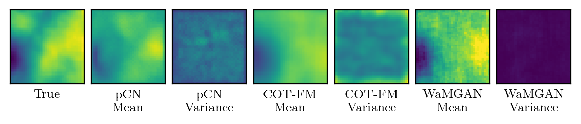
Figure 1: Results for the Darcy flow inverse problem. We compare the posterior mean and variance of our method (COT-FM) to pCN (Cotter et al., 2013) and WaMGAN (Hosseini et al., 2023).

We have thus far seen that the COT problem (11) admits a dynamical formulation (99), where one may take the underlying vector fields to be triangular. We use these results to design a principled model for conditional generation based on flow matching (Lipman et al., 2022; Albergo et al., 2023b). More specifically, recent work (Tong et al., 2023; Pooladian et al., 2023a) has proposed to couple the source and target measures in flow matching via optimal transport. We extend these techniques to the conditional setting.

In this section we make several simplifying assumptions. First, we use the squared-distance cost $|(y_{0},u_{0})-(y_{1},u_{1})|^{2}$ throughout (i.e. $p=2$). Second, we assume that $Y$ and $U$ are finite dimensional Euclidean spaces, but we emphasize that our techniques may be applied to infinite dimensional spaces under additional regularity assumptions (Kerrigan et al., 2023, 2022; Lim et al., 2023; Baldassari et al., 2024). Third, we assume that our source and target measures admit densities with respect to the Lebesgue measure on $Y\times U$. This is sufficient (Prop. 4) for the existence of a unique COT plan which is induced by a triangular map. We will henceforth, in an abuse of notation, identify measures with their densities.

Flow Matching.

We assume that we have access to samples $z_{0}=(y_{0},u_{0})\sim\eta(y_{0},u_{0})\in\mathbb{P}_{p}^{\mu}(Y\times U)$ from a source measure, and samples $z_{1}=(y_{1},u_{1})\sim\nu(y_{1},u_{1})\in\mathbb{P}_{p}^{\mu}(Y\times U)$ from a target measure. Let $z=(z_{0},z_{1})\sim\rho(z_{0},z_{1})\in\Pi(\eta,\nu)$ be any coupling of the source and target measure. Following Tong et al. (2023), we specify a collection of measures and vector fields via

$$\gamma_{t}(y,u\mid z)=\mathcal{N}\left(y,u\mid tz_{1}+(1-t)z_{0},C\right)$$ (102)

$$u_{t}(y,u\mid z)=z_{1}-z_{0}$$ (103)

where $C$ is any trace-class covariance operator (Da Prato and Zabczyk, 2014), e.g. $C=\sigma^{2}I$.

As is standard in flow matching (Lipman et al., 2022; Tong et al., 2023; Kerrigan et al., 2023), we obtain from Equations (102) and (103) a marginal measure $\gamma_{t}(y,u)$ and vector field $u_{t}(y,u)$ satisfying the continuity equation via

$$\gamma_{t}(y,u)=\int_{(Y\times U)^{2}}\gamma_{t}(y,u\mid z)\,\mathrm{d}\rho(z)$$ (104)

$$u_{t}(y,u)=\int_{(Y\times U)^{2}}u_{t}(y,u\mid z)\frac{\,\mathrm{d}\gamma_{t}(y,u\mid z)}{\,\mathrm{d}\gamma_{t}(y,u)}\,\mathrm{d}\rho(z).$$ (105)

To model the intractable $u_{t}(y,u)$, we minimize the loss

$$\mathcal{L}(\theta)=\mathbb{E}_{t,\rho(z),\gamma_{t}(y,u\mid z)}\left\lVert u^{\theta}(t,y,u)-u_{t}(y,u\mid z)\right\rVert^{2}$$ (106)

which has the same gradient (with respect to $\theta$ as the MSE loss to the true vector field of interest $u_{t}(y,u)$ (Tong et al., 2023, Theorem 3.2).

COT Flow Matching.

Figure 2: Further visualizations of our results on the Darcy flow inverse problem. The first row shows the ground-truth posterior. Row two shows samples obtained from out COT-FM method, and row three shows the same for WaMGAN (Hosseini et al., 2023). The prior and conditioning information are shown in the final two rows.

In the preceding section, $\rho(z)$ may be an arbitrary coupling between $\eta$ and $\nu$. Motivated by Propositions 1 and 4, we will choose $\rho$ to be a conditional optimal coupling, so that $(y_{0},u_{0},y_{1},u_{1})\sim\rho$ has the form $\left(y,u,y,T_{U}(y,u)\right)$. By Theorem 16 and Theorem 11, under such a $\rho$ the vector fields in Equation (103) and Equation (105) will be triangular. Thus, we parametrize our model $u^{\theta}$ to also be triangular. If the covariance operator $C$ in Equation (102) is taken such that $\text{tr}(C)\to 0$, then we recover the optimal path of measures given by the conditional Benamou-Brenier Theorem via a pointwise application of (Tong et al., 2023, Proposition 3.4).

Given a collection of samples $\{z_{0}^{i},z_{1}^{i}\}_{i=1}^{n}$ drawn from $\eta$ and $\nu$, we approximate a conditional optimal coupling $\rho$ using standard numerical techniques (e.g., those available in the POT package (Flamary et al., 2021)) with the cost function

$$c_{\epsilon}(y_{0},u_{0},y_{1},u_{1})=|y_{1}-y_{0}|^{2}+\epsilon|u_{1}-u_{0}|^{2}$$ (107)

for some $0<\epsilon\ll 1$. Intuitively, such a cost penalizes mass transfer along the $Y$ dimension, which is precisely the constraint sought in the COT problem (11). Hosseini et al. (2023, Prop. 3.11) show that as $\epsilon\downarrow 0$, we recover the true optimal triangular map. When our datasets are not too large, we precompute this COT coupling prior to training our flow matching model. Otherwise, we compute this COT coupling for each minibatch drawn at training time.

After training, we obtain a learned triangular vector field $u^{\theta}_{t}(y,u)$. Given an arbitrary fixed $y\in Y$, we may approximately sample from the target $\nu(u\mid y)$ by sampling $u_{0}\sim\eta(u_{0}\mid y)$ and numerically solving the corresponding differential equation. For some tasks, like domain translation, note that we are given a fixed $u_{0}$ of interest rather than sampling $u_{0}$ from the source. In these cases, we are effectively sampling from $\nu(u\mid y,u_{0})$.

Source Measure.

Our framework is agnostic to the choice of source measure $\eta$, allowing for great flexibility in the modeling process. The main requirement is that the $Y$-marginal of $\eta$ must match the $Y$-marginal of the target $\nu$. In some scenarios, this is trivially satisfied. For instance, if one is interested in using a source distribution which is simply random noise, one may take $\eta(y_{0},u_{0})=\pi^{Y}_{\#}\nu(y_{0})\eta_{U}(u_{0})$ to be the product of two independent distributions where $\eta_{U}(u)$ is arbitrary, e.g. Gaussian noise. Sampling from such an $\eta$ can be achieved by sampling noise from $\eta_{U}(u)$ and an independent $y$ from the target measure. We explore more complex choices for $\eta$ in Section 7.

7 Experiments

The following section is devoted to illustrate our methodology on a variety of different problems related to conditional simulation. First, we explore a likelihood-free inference problem in function space on a Darcy flow inverse problem. The dataset used in this case mirrors those in Hosseini et al. (2023), as we aim to directly compare with their Conditional Wasserstein Monge GAN (WaMGAN) method. In addition, we demonstrate our method on two unpaired image-to-image translation tasks (Nazarpour and Chen, 2017; Choi et al., 2020)

7.1 Bayesian Inverse Problems

In this experiment, we consider simulation-based posterior inference on the parameters characterizing a stochastic forward model, whose likelihood evaluation is intractable.

Darcy Flow

In this experiment the forward model corresponding to the 2D Darcy flow, an ellipitic PDE on a smooth domain $\Omega\subset\mathbb{R}^{d}$ characterized by a permeability field $\exp(u)$, a pressure field $\rho$, and a source term $f$:

$$-\text{div}\exp(u)\nabla\rho=f\quad\text{in}\quad\Omega,\qquad\rho=0\quad\text{on}\quad\partial\Omega.$$ (108)

For simplicity we denote the deterministic part of the forward model as $\mathfrak{F}:U\rightarrow Y$, and the stochasticity arises from only having access to noisy measurements $y=\mathfrak{F}(u)+\epsilon\in Y,$ where $\epsilon\sim\mathcal{N}(0,\sigma^{2}I)$. Although the general setting of the experiment corresponds to the one in Hosseini et al. (2023), we consider the more general task of performing posterior inference for $u$ when both $u$ and $y$ are observed at arbitrary resolutions, effectively posing the problem in function space. Hence, we consider $Y\subseteq\mathcal{Y}$, $U\subseteq\mathcal{U}$, where $\mathcal{Y},\mathcal{U}$ are infinite-dimensional Hilbert spaces. We remark that, although the measurements $Y$ are observed on a grid their resolution does not need to be fixed, allowing for training on observations at different resolutions. It follows that $\epsilon$ follows a Gaussian measure on $Y$ with a white noise kernel. Notice that although the conditional probability measure $\nu^{u}:=\pi^{U}_{\#}\nu$ is Gaussian, evaluating it requires simulating from Equation (108).

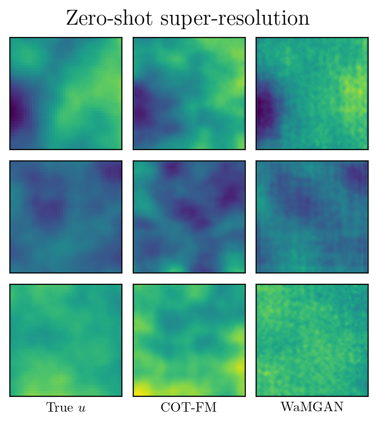
Figure 3: Zero-shot super-resolution on the Darcy flow inverse problem. Our model (COT-FM) is trained using a Fourier Neural Operator (Li et al., 2020), allowing us to generate samples at higher resolutions than available at training time. We compare to WaMGAN (Hosseini et al., 2023) trained with the same architechture.

We assign to $u_{1}$ a prior corresponding to the Gaussian measure $\mathcal{N}(0,C_{1})$, where $C_{1}$ corresponds to a symmetric, non-negative and trace-class covariance operator (Da Prato and Zabczyk, 2014). In order to obtain a dataset $\mathcal{D}_{1}=\{y_{1,i},u_{1,i}\}_{i=1}^{n}$ of samples on the target domain, we simulate $y_{1}$ from Equation (108) parameterizing the forward model with samples $u_{1}\sim\mathcal{N}(0,C_{1})$. We denote the target measure as $\nu$. We construct the source measure $\eta$ as the product measure $\mathcal{N}(0,C_{0})\times\mu$, where $C_{0}$ is symmetric, non-negative, trace-class and $\mu=\pi^{Y}_{\#}\eta$ corresponds to the marginal data distribution. The choice of picking $C_{0}\neq C_{1}$, while complicating the problem, reflects a scenario where we want to perform inference with a weakly informative prior that does not reflect the true data generating process. Notice that sampling from a conditional coupling $\gamma\in\Pi_{Y}(\eta,\nu)$ would still recover samples from the true posterior. Here, we assume that $C_{0},C_{1}$ are sufficiently regular such that the path of measures in Equation (104) is well-defined.

Our goal is to perform posterior sampling, that is sampling from the probability measure $\eta^{y}$ obtained by disintegration. Function-space Markov chain Monte Carlo approaches to solve this problem include the preconditioned Crank-Nicolson (pCN) (Cotter et al., 2013) and gradient-based methods such as the infinite-dimensional Metropolis-adjusted Langevin algorithm ($\infty-$MALA) (Beskos et al., 2008) and infinite-dimensional Hamiltonian Monte Carlo ($\infty-$HMC) (Beskos et al., 2011). In order to make learning feasible in this space we adapt the architecture of a Fourier Neural Operator (FNO) (Li et al., 2020) to accomodate for conditioning information observed at an arbitrary resolution. We do so by introducing a projection layer mapping the conditioning information to match the hidden channels of the input lifting block, and a pooling operation to project to the input dimensions. The two are then concatenated and passed through an FNO block mapping from $2\,\text{{hidden\_dim}}\times\text{{input\_dim}}$ to $\text{{hidden\_dim}}\times\text{{input\_dim}}$, before following the original architecture.

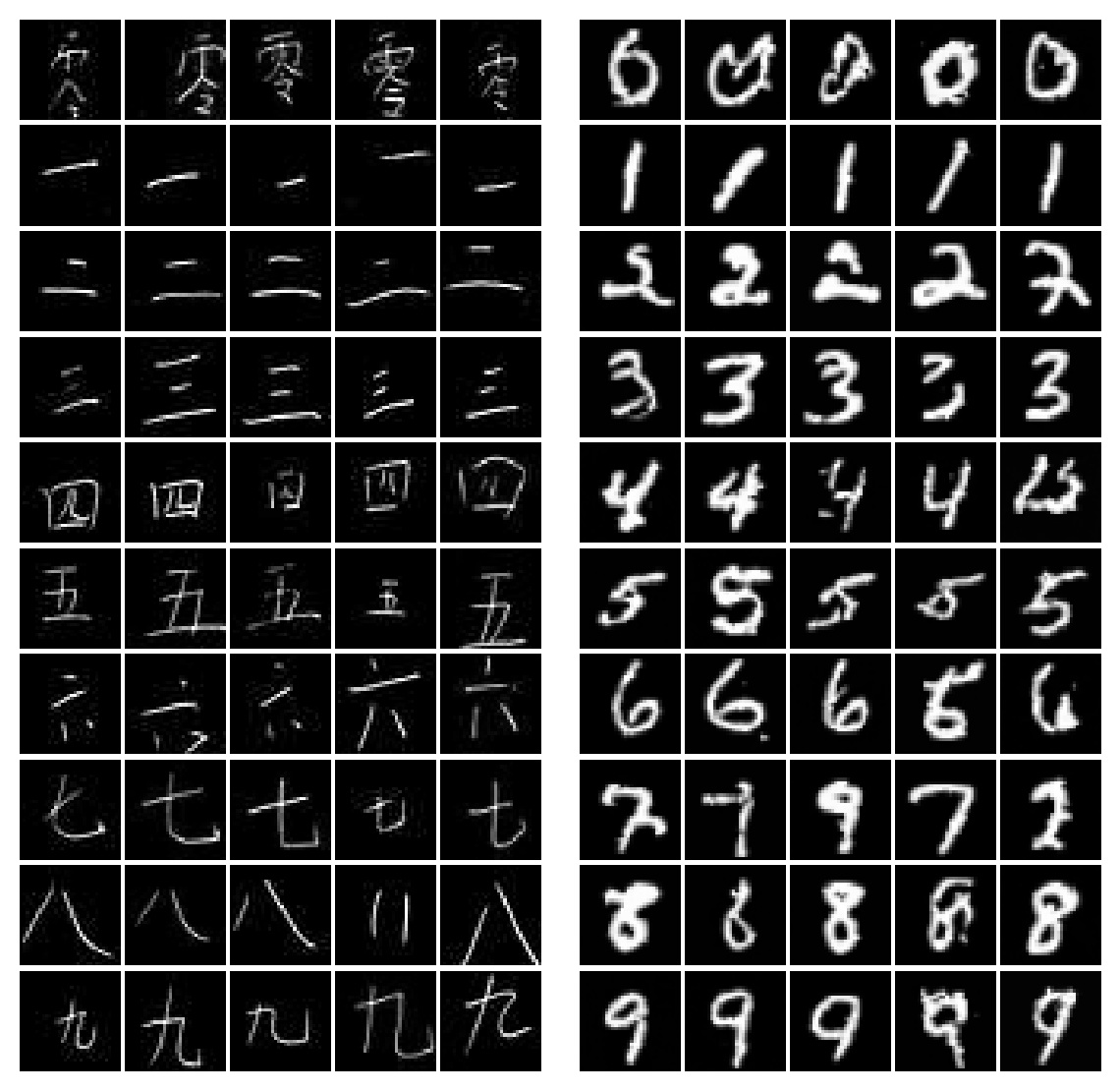
(a)

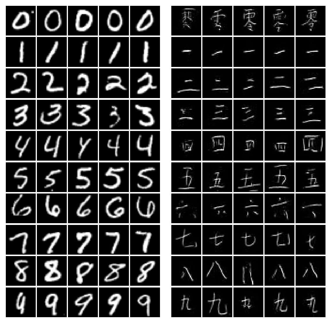
(b)

Figure 4: Samples from our model on a supervised image-to-image translation task, where translation is performed from Chinese MNIST to MNIST (a) and from MNIST to Chinese MNIST (b). This demonstrates that our method is able to use non-trivial source distributions and is able to successfully draw samples from the corresponding conditional measure.

The resulting amortized sampler, denoted for simplification by the mapping $(y,u_{0})\mapsto u_{1}=\tilde{T}_{U}(y,u_{0})$, will parameterize an approximate posterior measure. Notice that, in contrast to variational inference techniques, no distributional assumptions are made about the approximate posterior. In turn, integrals are obtained numerically by Monte Carlo sampling $K-$many samples from the prior, resulting in the approximation

$$\nu^{y}(f)\approx\int f\,\mathrm{d}\delta_{\tilde{T}_{U}(y,u_{0})}\,\mathrm{d}\mathcal{N}(0,C_{0})\approx\frac{1}{K}\sum^{K}_{k=1}f(\tilde{T}_{U}(y_{k},u_{0,k})),\quad\{u_{0,k}\}_{k=1}^{K}\overset{\text{i.i.d.}}{\sim}\mathcal{N}(0,C_{0}).$$ (109)

In Figure 1, we show an example of how our method compares to pCN and WaMGAN on recovering the posterior mean and variance on a given example. For a fair comparison and to ensure resolution-invariance, we used the same architecture for both neural models, with the discriminator having an additional layer projecting to a scalar value. However, the WaMGAN method used twice as many parameters as it requires two neural networks. Each statistic is computed on $2\times 10^{3}$ samples from each method. We showcase the ability of our method to perform zero-shot super-resolution in Figure 3. A random selection of samples from our method and from WaMGAN, as well as the prior sample and the different conditions used for generation, are displayed in Figure 2. Qualitatively, our samples appear to better match the true posterior compared to WaMGAN (Hosseini et al., 2023), while being cheaper to sample than pCN (Cotter et al., 2013).

7.2 Unpaired Image-to-Image Translation

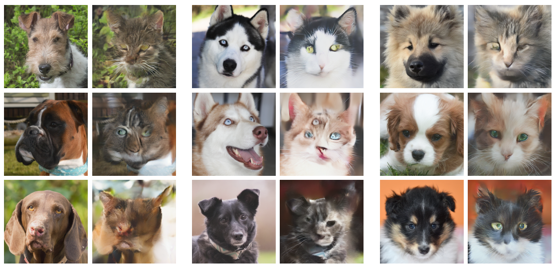
Figure 5: Uncurated sample from the test set of the Animal Faces HQ dataset (Choi et al., 2020) from the dogs class, translated to cats. These results demonstrate our method on an unsupervised image-to-image task, where we utilize a pre-trained content extractor.

We now demonstrate our method on an image-to-image translation task. In particular, in this section our source measures are distributions over images. The objective of domain translation is to convert information from one domain to another by adjusting domain-specific attributes, denoted style, while preserving the domain-invariant ones, denoted content (Isola et al., 2017). Semantic attributes can be associated with human-assigned labels (supervised) or inferred by a learning algorithm that learns domain-invariant representations of the data (unsupervised). Pseudocode is available in Appendix A.

Historically, the problem of domain translation was tackled through methods that heavily relied on parallel datasets—pairs of corresponding samples from the source and target domains. However, obtaining such paired datasets is often impractical or impossible in many real-world applications, prompting the shift towards methods that do not require paired data (unpaired domain translation) (Pang et al., 2021). Domain translation is possible for a learning algorithm if it satisfies cycle consistency, positing that translation of a source sample $u_{s}$ into a target sample $\hat{u}_{t}$ and then back to the source domain should recover $\hat{u}_{s}=u_{s}$, and the same shall hold by starting from a target sample. Notice that this property is achieved naturally by our model, and hence does not require additional terms in the loss as is the case for GAN- or VAE-based methods (Zhu et al., 2017; Isola et al., 2017; Liu et al., 2017).

Here, the space $U$ corresponds to the space of images. For the space $Y$, we explore two choices. First, if supervised information (i.e., a class label) is available, we take $Y$ to be the space of labels. In this setting, if the class distribution in both the source and target distribution is balanced, then the $Y$-marginals of the source and target measures match. When such information is not available, we extract semantic information from our images using a pre-trained encoder, mapping images to a latent space $Y$. In this case, we assume the encoding distribution matches across the source and target distributions. Exploring techniques for balancing this distribution is an interesting avenue for future work.

Supervised.

We showcase in Figure 4 the ability of our method to address the task of class-conditional image translation, using the MNIST and the Chinese MNIST (Nazarpour and Chen, 2017) datasets. The second dataset was preprocessed in order to center the images around their content, and both are reshaped to a resolution of $32\times 32$. The size of the training set was small enough for us to compute the empirical COT plan on the entire dataset, and pairs were resampled at each epoch. We parameterize the neural network in COT-FM with a UNet (Ronneberger et al., 2015), and we compute the $Y-$distance in the COT plan by taking the $L_{2}$ distance between one-hot encoded vectors for the labels. The UNet has hidden dimensionality of 128, and we use three downsampling/upsampling blocks with multipliers $(1,2,2)$. The optimizer is Adam (Kingma and Ba, 2014) with a learning rate of $10^{-4}$, at a batch size of 128 for $3\times 10^{5}$ training steps.

Unsupervised.

Samples are mapped into a shared representation space by a pre-trained feature extractor $\mathfrak{F}:\mathbb{R}^{d}\rightarrow[0,1]^{e}$, obtaining content variables $y=\mathfrak{F}(u)$. These effectively act as pseudo-labels when building the empirical COT matrix. In our example, we perform translation from the dogs class to the cats class in the AnimalFacesHQ dataset (Choi et al., 2020) and we use CLIP as our feature extractor (Radford et al., 2021) as found in the official Hugging Face repository in its version clip-vit-large-patch14. The training set is comprised of 5067 images of cats and 4680 images of dogs, enabling the computation of the COT plan in advance. As with the previous experiment, samples are repaired by sampling from the COT plan at each epoch. Images are observed at a native resolution of $512\times 512$, but to ease the memory requirements we employ another pre-trained encoder $\mathfrak{E}:\mathbb{R}^{d}\rightarrow\mathbb{R}^{z}$ for dimensionality reduction, effectively performing flow matching in latent space (Dao et al., 2023). The procedure is detailed in Algorithm 1. We take the encoder $\mathfrak{E}$ to be the variational autoencoder (Kingma and Welling, 2013) from Stable Diffusion v2.1, enabling training of the COT-FM network at a dimensionality of $4\times 64\times 64$. We use the Adam optimizer (Kingma and Ba, 2014) with a learning rate of $2\times 10^{-4}$, with a batch size of 32 for $4\times 10^{5}$ training steps. We show several uncurated conditional samples from our model in Figure 5.

8 Conclusion

We analyze conditional optimal transport from a geometric and dynamical point of view. Our analysis culminates in the characterization of absolutely continuous curves of measures in a conditional Wasserstein space, resulting in a conditional analog of the Benamou-Brenier Theorem. We use these result to build on the framework of triangular transport and flow matching to develop simulation-free methods for conditional generative models. Our methods are applicable across a wide class of problems, and we demonstrate our methodology on an infinite-dimensional Bayesian inverse problem as well as image translation tasks.

Acknowledgments

This research was supported by the Hasso Plattner Institute (HPI) Research Center in Machine Learning and Data Science at the University of California, Irvine, by the National Science Foundation under award 1900644, and by the National Institutes of Health under award R01-LM013344.

Appendix A Pseudocode

1:  Input: Data $\{u_{0,i},u_{1,i}\}_{i=1}^{B}\sim\gamma^{\star}_{COT}$, pretrained content extractor $\mathfrak{F}$, interpolant network $v_{\theta}$, pretrained encoder $\mathfrak{E}$ (optional).

2:  Initialize: $\mathcal{L}=0$

3:  $\{y_{0,i},y_{1,i}\}_{i=1}^{B}\leftarrow\{\mathfrak{F}(u_{0,i}),\mathfrak{F}(u_{1,i})\}_{i=1}^{B}$

4:  if  $\mathfrak{E}$ is given  then

5:     $\{u_{0,i},u_{1,i}\}_{i=1}^{B}\leftarrow\{\mathfrak{E}(u_{0,i}),\mathfrak{E}(u_{1,i})\}_{i=1}^{B}$

6:  end if

7:  for $i=1,\dots,B$ do

8:     Sample $t_{i}\sim\mathcal{U}([0,1])$

9:     Interpolate: $u_{t,i}=(1-t_{i})u_{0,i}+t_{i}u_{1,i}$

10:     Evaluate interpolant network:

$$\hat{v}_{t_{i}}^{0}=v_{\theta}(u_{t,i},t_{i},y_{0,i}),\quad\hat{v}_{t_{i}}^{1}=v_{\theta}(u_{t,i},t_{i},y_{1,i})$$

11:     Compute interpolant loss: $\begin{aligned} \mathcal{L}\mathrel{+}=&\left(\left\lVert\hat{v}_{t_{i}}^{0}-(u_{1,i}-u_{0,i})\right\rVert_{2}^{2}+\left\lVert\hat{v}_{t_{i}}^{1}-(u_{1,i}-u_{0,i})\right\rVert_{2}^{2}\right)\end{aligned}$

112:  end for

213:  $\theta_{\text{new}}\leftarrow$ OptimizerStep$(\nabla_{\theta}\mathcal{L})$

Algorithm 1 DCOT Flow for Unsupervised Image-to-Image Translation, Training Step

References

• Albergo and Vanden-Eijnden (2022) MichaelΒ S Albergo and Eric Vanden-Eijnden. Building normalizing flows with stochastic interpolants. arXiv preprint arXiv:2209.15571, 2022.
• Albergo etΒ al. (2023a) MichaelΒ S Albergo, NicholasΒ M Boffi, and Eric Vanden-Eijnden. Stochastic interpolants: A unifying framework for flows and diffusions. arXiv preprint arXiv:2303.08797, 2023a.
• Albergo etΒ al. (2023b) MichaelΒ S Albergo, Mark Goldstein, NicholasΒ M Boffi, Rajesh Ranganath, and Eric Vanden-Eijnden. Stochastic interpolants with data-dependent couplings. arXiv preprint arXiv:2310.03725, 2023b.
• Ambrosio etΒ al. (2005) Luigi Ambrosio, Nicola Gigli, and Giuseppe SavarΓ©. Gradient flows: in metric spaces and in the space of probability measures. Springer Science & Business Media, 2005.
• Ambrosio etΒ al. (2013) Luigi Ambrosio, Alberto Bressan, Dirk Helbing, Axel Klar, Enrique Zuazua, Luigi Ambrosio, and Nicola Gigli. A user’s guide to optimal transport. Modelling and Optimisation of Flows on Networks: Cetraro, Italy 2009, Editors: Benedetto Piccoli, Michel Rascle, pages 1–155, 2013.
• Amos etΒ al. (2023) Brandon Amos etΒ al. Tutorial on amortized optimization. Foundations and Trends in Machine Learning, 16(5):592–732, 2023.
• Baldassari etΒ al. (2024) Lorenzo Baldassari, Ali Siahkoohi, Josselin Garnier, Knut Solna, and MaartenΒ V deΒ Hoop. Conditional score-based diffusion models for Bayesian inference in infinite dimensions. Advances in Neural Information Processing Systems, 36, 2024.
• Baptista etΒ al. (2020) Ricardo Baptista, Bamdad Hosseini, NikolaΒ B Kovachki, and Youssef Marzouk. Conditional sampling with monotone GANs: from generative models to likelihood-free inference. arXiv preprint arXiv:2006.06755, 2020.
• Barboni etΒ al. (2024) RaphaΓ«l Barboni, Gabriel PeyrΓ©, and FranΓ§ois-Xavier Vialard. Understanding the training of infinitely deep and wide ResNets with conditional optimal transport. arXiv preprint arXiv:2403.12887, 2024.
• Benamou and Brenier (2000) Jean-David Benamou and Yann Brenier. A computational fluid mechanics solution to the Monge-Kantorovich mass transfer problem. Numerische Mathematik, 84(3):375–393, 2000.
• Beskos etΒ al. (2008) Alexandros Beskos, Gareth Roberts, Andrew Stuart, and Jochen Voss. MCMC methods for diffusion bridges. Stochastics and Dynamics, 8(03):319–350, 2008.
• Beskos etΒ al. (2011) Alexandros Beskos, FrankΒ J Pinski, JesΓΊsΒ MarΔ±a Sanz-Serna, and AndrewΒ M Stuart. Hybrid Monte Carlo on Hilbert spaces. Stochastic Processes and their Applications, 121(10):2201–2230, 2011.
• Bogachev and Ruas (2007) VladimirΒ Igorevich Bogachev and Maria AparecidaΒ Soares Ruas. Measure Theory, volumeΒ 2. Springer, 2007.
• Bunne etΒ al. (2022a) Charlotte Bunne, Andreas Krause, and Marco Cuturi. Supervised training of conditional monge maps. Advances in Neural Information Processing Systems, 35:6859–6872, 2022a.
• Bunne etΒ al. (2022b) Charlotte Bunne, Laetitia Papaxanthos, Andreas Krause, and Marco Cuturi. Proximal optimal transport modeling of population dynamics. In International Conference on Artificial Intelligence and Statistics, pages 6511–6528. PMLR, 2022b.
• Carlier etΒ al. (2016) Guillaume Carlier, Victor Chernozhukov, and Alfred Galichon. Vector quantile regression: An optimal transport approach. The Annals of Statistics, 44(3):1165 – 1192, 2016. doi: 10.1214/15-AOS1401. URL https://doi.org/10.1214/15-AOS1401.
• Chemseddine etΒ al. (2024) Jannis Chemseddine, Paul Hagemann, Christian Wald, and Gabriele Steidl. Conditional Wasserstein distances with applications in Bayesian OT flow matching. arXiv preprint arXiv:2403.18705, 2024.
• Chen and Lipman (2023) RickyΒ TQ Chen and Yaron Lipman. Riemannian flow matching on general geometries. arXiv preprint arXiv:2302.03660, 2023.
• Choi etΒ al. (2020) Yunjey Choi, Youngjung Uh, Jaejun Yoo, and Jung-Woo Ha. Stargan v2: Diverse image synthesis for multiple domains. In Proceedings of the IEEE/CVF Conference on Computer Vision and Pattern Recognition, pages 8188–8197, 2020.
• Cotter etΒ al. (2013) S.Β L. Cotter, G.Β O. Roberts, A.Β M. Stuart, and D.Β White. MCMC methods for functions: Modifying old algorithms to make them faster. Statistical Science, 28(3):424 – 446, 2013.
• Cranmer etΒ al. (2020) Kyle Cranmer, Johann Brehmer, and Gilles Louppe. The frontier of simulation-based inference. Proceedings of the National Academy of Sciences, 117(48):30055–30062, 2020.
• DaΒ Prato and Zabczyk (2014) Giuseppe DaΒ Prato and Jerzy Zabczyk. Stochastic Equations in Infinite Dimensions. Cambridge University Press, 2014.
• Dao etΒ al. (2023) Quan Dao, Hao Phung, Binh Nguyen, and Anh Tran. Flow matching in latent space. arXiv preprint arXiv:2307.08698, 2023.
• Dashti and Stuart (2013) Masoumeh Dashti and AndrewΒ M Stuart. The Bayesian approach to inverse problems. arXiv preprint arXiv:1302.6989, 2013.
• Davtyan etΒ al. (2023) Aram Davtyan, Sepehr Sameni, and Paolo Favaro. Efficient video prediction via sparsely conditioned flow matching. In Proceedings of the IEEE/CVF International Conference on Computer Vision, pages 23263–23274, 2023.
• Finlay etΒ al. (2020) Chris Finlay, JΓΆrn-Henrik Jacobsen, Levon Nurbekyan, and Adam Oberman. How to train your neural ODE: the world of Jacobian and kinetic regularization. In International Conference on Machine Learning, pages 3154–3164. PMLR, 2020.
• Flamary etΒ al. (2021) RΓ©mi Flamary, Nicolas Courty, Alexandre Gramfort, MokhtarΒ Z. Alaya, AurΓ©lie Boisbunon, Stanislas Chambon, Laetitia Chapel, Adrien Corenflos, Kilian Fatras, Nemo Fournier, LΓ©o Gautheron, NathalieΒ T.H. Gayraud, Hicham Janati, Alain Rakotomamonjy, Ievgen Redko, Antoine Rolet, Antony Schutz, Vivien Seguy, DanicaΒ J. Sutherland, Romain Tavenard, Alexander Tong, and Titouan Vayer. POT: Python optimal transport. Journal of Machine Learning Research, 22(78):1–8, 2021. URL http://jmlr.org/papers/v22/20-451.html.
• Gebhard etΒ al. (2023) TimothyΒ D Gebhard, Jonas Wildberger, Maximilian Dax, Daniel Angerhausen, SaschaΒ P Quanz, and Bernhard SchΓΆlkopf. Inferring atmospheric properties of exoplanets with flow matching and neural importance sampling. arXiv preprint arXiv:2312.08295, 2023.
• Goodfellow etΒ al. (2014) Ian Goodfellow, Jean Pouget-Abadie, Mehdi Mirza, Bing Xu, David Warde-Farley, Sherjil Ozair, Aaron Courville, and Yoshua Bengio. Generative adversarial nets. Advances in Neural Information Processing Systems, 27, 2014.
• Ho etΒ al. (2020) Jonathan Ho, Ajay Jain, and Pieter Abbeel. Denoising diffusion probabilistic models. Advances in Neural Information Processing Systems, 33:6840–6851, 2020.
• Hosseini etΒ al. (2023) Bamdad Hosseini, AlexanderΒ W Hsu, and Amirhossein Taghvaei. Conditional optimal transport on function spaces. arXiv preprint arXiv:2311.05672, 2023.
• Huguet etΒ al. (2022) Guillaume Huguet, DanielΒ Sumner Magruder, Alexander Tong, Oluwadamilola Fasina, Manik Kuchroo, Guy Wolf, and Smita Krishnaswamy. Manifold interpolating optimal-transport flows for trajectory inference. Advances in Neural Information Processing Systems, 35:29705–29718, 2022.
• Isobe etΒ al. (2024) Noboru Isobe, Masanori Koyama, Kohei Hayashi, and Kenji Fukumizu. Extended flow matching: a method of conditional generation with generalized continuity equation. arXiv preprint arXiv:2402.18839, 2024.
• Isola etΒ al. (2017) Phillip Isola, Jun-Yan Zhu, Tinghui Zhou, and AlexeiΒ A Efros. Image-to-image translation with conditional adversarial networks. In Proceedings of the IEEE/CVF Conference on Computer Vision and Pattern Recognition, 2017.
• Kerrigan etΒ al. (2022) Gavin Kerrigan, Justin Ley, and Padhraic Smyth. Diffusion generative models in infinite dimensions. arXiv preprint arXiv:2212.00886, 2022.
• Kerrigan etΒ al. (2023) Gavin Kerrigan, Giosue Migliorini, and Padhraic Smyth. Functional flow matching. arXiv preprint arXiv:2305.17209, 2023.
• Kingma and Ba (2014) DiederikΒ P Kingma and Jimmy Ba. Adam: A method for stochastic optimization. arXiv preprint arXiv:1412.6980, 2014.
• Kingma and Welling (2013) DiederikΒ P Kingma and Max Welling. Auto-encoding variational Bayes. arXiv preprint arXiv:1312.6114, 2013.
• Korotin etΒ al. (2022) Alexander Korotin, Daniil Selikhanovych, and Evgeny Burnaev. Neural optimal transport. arXiv preprint arXiv:2201.12220, 2022.
• Lee etΒ al. (2023) Sangyun Lee, Beomsu Kim, and JongΒ Chul Ye. Minimizing trajectory curvature of ode-based generative models. In International Conference on Machine Learning, pages 18957–18973. PMLR, 2023.
• Li etΒ al. (2020) Zongyi Li, Nikola Kovachki, Kamyar Azizzadenesheli, Burigede Liu, Kaushik Bhattacharya, Andrew Stuart, and Anima Anandkumar. Fourier neural operator for parametric partial differential equations. arXiv preprint arXiv:2010.08895, 2020.
• Lim etΒ al. (2023) JaeΒ Hyun Lim, NikolaΒ B Kovachki, Ricardo Baptista, Christopher Beckham, Kamyar Azizzadenesheli, Jean Kossaifi, Vikram Voleti, Jiaming Song, Karsten Kreis, Jan Kautz, etΒ al. Score-based diffusion models in function space. arXiv preprint arXiv:2302.07400, 2023.
• Lipman etΒ al. (2022) Yaron Lipman, RickyΒ TQ Chen, Heli Ben-Hamu, Maximilian Nickel, and Matthew Le. Flow matching for generative modeling. In The Eleventh International Conference on Learning Representations, 2022.
• Liu etΒ al. (2017) Ming-Yu Liu, Thomas Breuel, and Jan Kautz. Unsupervised image-to-image translation networks. Advances in Neural Information Processing Systems, 30, 2017.
• Liu etΒ al. (2022) Xingchao Liu, Chengyue Gong, and Qiang Liu. Flow straight and fast: Learning to generate and transfer data with rectified flow. arXiv preprint arXiv:2209.03003, 2022.
• Makkuva etΒ al. (2020) Ashok Makkuva, Amirhossein Taghvaei, Sewoong Oh, and Jason Lee. Optimal transport mapping via input convex neural networks. In International Conference on Machine Learning, pages 6672–6681. PMLR, 2020.
• McCann (1997) RobertΒ J McCann. A convexity principle for interacting gases. Advances in Mathematics, 128(1):153–179, 1997.
• Nazarpour and Chen (2017) KΒ Nazarpour and MΒ Chen. Handwritten Chinese Numbers. 1 2017. doi: 10.17634/137930-3. URL https://data.ncl.ac.uk/articles/dataset/Handwritten_Chinese_Numbers/10280831.
• Neklyudov etΒ al. (2023) Kirill Neklyudov, Rob Brekelmans, Alexander Tong, Lazar Atanackovic, Qiang Liu, and Alireza Makhzani. A computational framework for solving Wasserstein Lagrangian flows. arXiv preprint arXiv:2310.10649, 2023.
• Onken etΒ al. (2021) Derek Onken, SamyΒ Wu Fung, Xingjian Li, and Lars Ruthotto. Ot-flow: Fast and accurate continuous normalizing flows via optimal transport. In Proceedings of the AAAI Conference on Artificial Intelligence, pages 9223–9232, 2021.
• Pang etΒ al. (2021) Yingxue Pang, Jianxin Lin, Tao Qin, and Zhibo Chen. Image-to-image translation: Methods and applications. IEEE Transactions on Multimedia, 24:3859–3881, 2021.
• Papamakarios etΒ al. (2021) George Papamakarios, Eric Nalisnick, DaniloΒ Jimenez Rezende, Shakir Mohamed, and Balaji Lakshminarayanan. Normalizing flows for probabilistic modeling and inference. Journal of Machine Learning Research, 22(57):1–64, 2021.
• Pooladian etΒ al. (2023a) Aram-Alexandre Pooladian, Heli Ben-Hamu, Carles Domingo-Enrich, Brandon Amos, Yaron Lipman, and Ricky Chen. Multisample flow matching: Straightening flows with minibatch couplings. arXiv preprint arXiv:2304.14772, 2023a.
• Pooladian etΒ al. (2023b) Aram-Alexandre Pooladian, Carles Domingo-Enrich, RickyΒ TQ Chen, and Brandon Amos. Neural optimal transport with lagrangian costs. In ICML Workshop on New Frontiers in Learning, Control, and Dynamical Systems, 2023b.
• Radford etΒ al. (2021) Alec Radford, JongΒ Wook Kim, Chris Hallacy, Aditya Ramesh, Gabriel Goh, Sandhini Agarwal, Girish Sastry, Amanda Askell, Pamela Mishkin, Jack Clark, etΒ al. Learning transferable visual models from natural language supervision. In International Conference on Machine Learning, pages 8748–8763. PMLR, 2021.
• Ronneberger etΒ al. (2015) Olaf Ronneberger, Philipp Fischer, and Thomas Brox. U-net: Convolutional networks for biomedical image segmentation. In Medical image computing and computer-assisted intervention–MICCAI 2015: 18th international conference, Munich, Germany, October 5-9, 2015, proceedings, part III 18, pages 234–241. Springer, 2015.
• Santambrogio (2015) Filippo Santambrogio. Optimal transport for applied mathematicians. BirkΓ€user, NY, 55(58-63):94, 2015.
• Song etΒ al. (2020) Yang Song, Jascha Sohl-Dickstein, DiederikΒ P Kingma, Abhishek Kumar, Stefano Ermon, and Ben Poole. Score-based generative modeling through stochastic differential equations. arXiv preprint arXiv:2011.13456, 2020.
• Taghvaei and Jalali (2019) Amirhossein Taghvaei and Amin Jalali. 2-Wasserstein approximation via restricted convex potentials with application to improved training for GANs. arXiv preprint arXiv:1902.07197, 2019.
• Tong etΒ al. (2020) Alexander Tong, Jessie Huang, Guy Wolf, David VanΒ Dijk, and Smita Krishnaswamy. Trajectorynet: A dynamic optimal transport network for modeling cellular dynamics. In International Conference on Machine Learning, pages 9526–9536. PMLR, 2020.
• Tong etΒ al. (2023) Alexander Tong, Nikolay Malkin, Guillaume Huguet, Yanlei Zhang, Jarrid Rector-Brooks, Kilian Fatras, Guy Wolf, and Yoshua Bengio. Improving and generalizing flow-based generative models with minibatch optimal transport. In ICML Workshop on New Frontiers in Learning, Control, and Dynamical Systems, 2023.
• Villani etΒ al. (2009) CΓ©dric Villani etΒ al. Optimal Transport: Old and New, volume 338. Springer, 2009.
• Wang etΒ al. (2023) ZheyuΒ Oliver Wang, Ricardo Baptista, Youssef Marzouk, Lars Ruthotto, and Deepanshu Verma. Efficient neural network approaches for conditional optimal transport with applications in Bayesian inference. arXiv preprint arXiv:2310.16975, 2023.
• Zhu etΒ al. (2017) Jun-Yan Zhu, Taesung Park, Phillip Isola, and AlexeiΒ A Efros. Unpaired image-to-image translation using cycle-consistent adversarial networks. In Proceedings of the IEEE/CVF Conference on Computer Vision and Pattern Recognition, pages 2223–2232, 2017.