Large sieve inequalities for exceptional Maass forms and applications

Abstract.

We prove new large sieve inequalities for the Fourier coefficients $\rho_{j\mathfrak{a}}(n)$ of exceptional Maass forms of a given level, weighted by sequences $(a_{n})$ with sparse Fourier transforms – including two key types of sequences that arise in the dispersion method. These give the first savings in the exceptional spectrum for the critical case of sequences as long as the level, and lead to improved bounds for various multilinear forms of Kloosterman sums.

We give three applications and suggest other likely consequences. We show that both primes and smooth numbers are equidistributed in arithmetic progressions to moduli up to $x^{5/8-o(1)}$, using triply-well-factorable weights for the primes; this completely eliminates the dependency on Selberg’s eigenvalue conjecture in previous results of Lichtman and the author. Separately, we show that the greatest prime factor of $n^{2}+1$ is infinitely often greater than $n^{1.3}$, improving Merikoski’s $n^{1.279}$.

1. Introduction

Let $m,n,c\in\mathbb{Z}$ with $c\geq 1$, and consider the classical Kloosterman sums

$$S(m,n;c):=\sum_{x\in(\mathbb{Z}/c\mathbb{Z})^{\times}}e\left(\frac{mx+n\overline{x}}{c}\right),$$ (1.1)

where $e(\alpha):=\exp(2\pi i\alpha)$ and $x\overline{x}\equiv 1\ (\textnormal{mod }c)$. A great number of results in analytic number theory [3, 25, 11, 12, 57, 14, 46, 47, 48, 8, 49, 43, 50, 59] rely on bounding exponential sums of the form

$$\sum_{m\sim M}a_{m}\sum_{n\sim N}b_{n}\sum_{(c,r)=1}g\left(\frac{c}{C}\right)S(m\overline{r},\pm n;sc),$$ (1.2)

where $(a_{m})$ and $(b_{n})$ are rough sequences of complex numbers, $g$ is a compactly-supported smooth function, and $r,s$ are coprime positive integers; one can often (but not always [49, 8, 46]) leverage some additional averaging over $r$ and $s$, if one of the sequences $(a_{m}),(b_{n})$ is independent of $r,s$.

Bounds for sums like 1.2 are typically obtained by the spectral theory of automorphic forms [36, 35], following Deshouillers–Iwaniec [9]. This allows one to bound 1.2 by certain averages of the sequences $(a_{m})$, $(b_{n})$ with the Fourier coefficients of automorphic forms for $\Gamma_{0}(rs)$. Often in applications, the limitation in these bounds comes from our inability to rule out the existence of exceptional Maass cusp forms, corresponding to exceptional eigenvalues $\lambda\in(0,1/4)$ of the hyperbolic Laplacian. This is measured by a parameter $\theta=\max_{\lambda}\sqrt{\max(0,1-4\lambda)}$, using Deshouillers–Iwaniec’s original normalization; under Selberg’s eigenvalue conjecture there would be no exceptional eigenvalues [53], so one could take $\theta=0$. But unconditionally, the record is Kim–Sarnak’s bound $\theta\leq 7/32$, based on the automorphy of symmetric fourth power $L$-functions [39, Appendix 2].

This creates a power-saving gap between the best conditional and unconditional results in various arithmetic problems [8, 49, 57, 43, 50, 14]. Improvements to the dependency on $\theta$, which help narrow this gap, come from large sieve inequalities for the Fourier coefficients of exceptional Maass cusp forms (see [9, Theorems 5, 6, 7] and their optimizations in [12, 43, 50]), which function as weak on-average substitutes for Selberg’s eigenvalue conjecture. However, in the key setting of fixed $r,s$ and sequences $(a_{n})$ of length $N\approx rs$, no such savings were previously available.

Luckily, for many of the most important applications, we don’t need to handle 1.2 for completely arbitrary sequences, but only for those arising from variations of Linnik’s dispersion method [44, 26, 3, 4, 5]; these are roughly of the form

$$a_{m}=e(m\alpha)\qquad\qquad\text{and}\qquad\qquad b_{n}=\sum_{\begin{subarray}{c}h_{1},h_{2}\sim H\\ h_{1}\ell_{1}-h_{2}\ell_{2}=n\end{subarray}}1,$$ (1.3)

for $\alpha\in\mathbb{R}/\mathbb{Z}$ and $\ell_{1}\asymp\ell_{2}\asymp H$ with $(\ell_{1},\ell_{2})=1$. Our main results in this paper are new large sieve inequalities for such sequences, whose Fourier transforms obey strong concentration conditions. These are obtained by combining the framework of Deshouillers–Iwaniec with combinatorial ideas – specifically, with new estimates for bilinear (vertical) sums of Kloosterman sums, stemming from a counting argument of Cilleruelo–Garaev [7]. The resulting improved bounds for 1.2 have natural ramifications to the equidistribution of primes and smooth numbers in arithmetic progressions to large moduli, as well as to the greatest prime factors of quadratic polynomials.

Figure 1. Structure of paper (arrows signify logical implications).

Figure 1 summarizes the results outlined above, which go from “counting problems” (on the top row), to exponential sums (middle row), to automorphic forms (bottom row), and then backwards. The transition between the first two rows is mostly elementary (using successive applications of Poisson summation, Cauchy–Schwarz, combinatorial decompositions, and/or sieve methods), while the transition between the last two rows uses the Kuznetsov trace formula [41, 9] from F.

1.1. Applications

Before we dive into the large sieve inequalities, let us motivate our discussion with the aforementioned applications. We begin with the following simple-to-state result.

Theorem 1.1 (Greatest prime factor of $n^{2}+1$).

For infinitely many positive integers $n$, the largest prime factor of $n^{2}+1$ is greater than $n^{1.3}$.

This makes progress on a longstanding problem, approximating the famous conjecture that there exist infinitely many primes of the form $n^{2}+1$. Back in 1967, Hooley [33] proved the same result with an exponent of $1.1001$, using the Weil bound for Kloosterman sums. In 1982, Deshouillers–Iwaniec [10] used their bounds on multilinear forms of Kloosterman sums [9] to improve this substantially, up to an exponent of $1.2024$. More recently, using Kim–Sarnak’s bound $\theta\leq 7/32$ from [39, Appendix 2], de la Bretèche and Drappeau optimized the exponent to $1.2182$. Finally, Merikoski [49] proved a new bilinear estimate (still relying on the bounds of Deshouillers–Iwaniec [9]), and used Harman’s sieve to reach the exponent $1.279$. Assuming Selberg’s eigenvalue conjecture, Merikoski also reached the conditional exponent $1.312$, which leaves a gap from our unconditional result.

With our large sieve inequalities (Theorems 1.4 and 1.5), we can improve the arithmetic information due to both Bretèche–Drappeau [8] and Merikoski [49], leading to the improvement in Theorem 1.1.

Next, we turn to equidistribution estimates for primes in arithmetic progressions with moduli beyond the square-root barrier [3, 4, 5, 46, 47, 48, 43], which have been critical inputs to sieve theory methods [61, 45, 51, 42, 43]. We use the standard notations

$$\pi(x):=\#\{\text{prime }p\leq x\}\qquad\quad\text{and}\qquad\quad\pi(x,q;a):=\#\{\text{prime }p\leq x:p\equiv a\ (\textnormal{mod }q)\},$$

recalling that the Siegel–Walfisz theorem gives the pointwise asymptotic $\pi(x,q;a)\sim\frac{\pi(x)}{\varphi(q)}$ in the small range $q\leq(\log x)^{A}$. The Generalized Riemann Hypothesis would improve this to $q\leq x^{1/2}/(\log x)^{B}$.

Theorem 1.2 (Primes in arithmetic progressions to large moduli).

Let $a\in\mathbb{Z}\setminus\{0\}$, $A,\varepsilon>0$, $x\geq 2$, and suppose that either:

• $Q\leq x^{5/8-\varepsilon}$, and $(\lambda_{q})$ are triply-well-factorable weights of level $Q$, or

• $Q\leq x^{3/5-\varepsilon}$, and $(\lambda_{q})$ are the well-factorable upper bound linear sieve weights of level $Q$.

(See Definitions 6.5 and 6.7 and their references.) Then one has

$$\sum_{\begin{subarray}{c}q\leq Q\\ (q,a)=1\end{subarray}}\lambda_{q}\left(\pi(x;q,a)-\frac{\pi(x)}{\varphi(q)}\right)\ll_{\varepsilon,A,a}\frac{x}{(\log x)^{A}}.$$ (1.4)

The celebrated Bombieri–Vinogradov theorem [2, 58] implies this result in the range $Q\leq x^{1/2-o(1)}$, with arbitrary weights $(\lambda_{q})$. This is as good as the best results assuming the Generalized Riemann Hypothesis, when such an average over $q$ is available; in particular, the Bombieri–Vinogradov theorem was enough to prove the existence of infinitely many bounded gaps between primes [45, 51]. It is believed [16] that the same should hold true for all $Q\leq x^{1-o(1)}$, which would imply the existence of infinitely many pairs of primes with distance at most $6$ [51, 45].

Surprisingly, since the outstanding work of Fouvry [18, 20, 19, 17], Fouvry–Iwaniec [21, 22], and Bombieri–Friedlander–Iwaniec [3, 4, 5], we have been able to overcome the barrier at $x^{1/2}$ up to various restrictions: fixing the residue $a$, summing over “most” moduli $q\leq Q$, and/or using special weights $(\lambda_{q})$; we also mention the more recent works of Zhang [61] and Maynard [46, 47, 48]. Such results, going “beyond” the Riemann hypothesis on average, are based on equidistribution estimates for various convolutions of sequences, and ultimately rely on bounding sums of Kloosterman sums.

In the setting of triply-well-factorable weights and linear sieve weights, Maynard [47] proved equidistribution results handling moduli up to $x^{3/5-o(1)}$ and $x^{7/12-o(1)}$ (which we improve to $x^{5/8-o(1)}$, respectively $x^{3/5-o(1)}$ above). Lichtman [43] then used optimized Deshouillers–Iwaniec estimates, via Kim–Sarnak’s bound [39], to improve the exponent for triply-well-factorable weights to $66/107-o(1)\approx 0.6168$, and up to $5/8-o(1)=0.625-o(1)$ assuming Selberg’s eigenvalue conjecture.

Fortunately, our large sieve inequalities and their consequences about sums of Kloosterman sums are just enough to completely remove the dependency on Selberg’s eigenvalue conjecture, reaching the exponents of $5/8-o(1)$ and $3/5-o(1)$ from Theorem 1.2 unconditionally.

The analogous equidistribution problem for smooth numbers [25, 11] concerns the quantities

$$\begin{gathered}\Psi(x,y):=\#\{y\text{-smooth }n\leq x\},\qquad\quad\Psi_{q}(x,y):=\#\{y\text{-smooth }n\leq x:(n,q)=1\},\\ \Psi(x,y;a,q):=\#\{y\text{-smooth }n\leq x:n\equiv a\ (\textnormal{mod }q)\},\end{gathered}$$ (1.5)

where a positive integer is called $y$-smooth if and only if all of its prime factors are $\leq y$. We can now state our third and final application, which uses arbitrary weights (i.e., absolute values).

Theorem 1.3 (Smooth numbers in arithmetic progressions to large moduli).

Let $a\in\mathbb{Z}\setminus\{0\}$ and $A,\varepsilon>0$, $x\geq 2$. Then there exists a large enough $C(a,A,\varepsilon)>0$ such that for any $y\in[(\log x)^{C},x^{1/C}]$ and $Q\leq x^{5/8-\varepsilon}$, one has

$$\sum_{\begin{subarray}{c}q\leq Q\\ (q,a)=1\end{subarray}}\left|\Psi(x,y;a,q)-\frac{\Psi_{q}(x,y)}{\varphi(q)}\right|\ll_{\varepsilon,A,a}\frac{\Psi(x,y)}{(\log x)^{A}}.$$

The analogue of Bombieri–Vinogradov’s theorem in this setting, with a barrier at $Q\leq x^{1/2-o(1)}$, is due to Granville [29, 30]. Fouvry–Tenenbaum [25] raised the level of distribution to $x^{3/5-o(1)}$ in a weak sense, with an upper bound of $x(\log x)^{-A}$; Drappeau later [11] strengthened the bound to $\Psi(x,y)/(\log x)^{A}$ in the same range $Q\leq x^{3/5-o(1)}$. Using a different arrangement of exponential sums and optimized Deshouillers–Iwaniec estimates, the author [50] recently improved the exponent to $66/107-o(1)\approx 0.6168$, and to $5/8-o(1)=0.625-o(1)$ assuming Selberg’s eigenvalue conjecture.

As in the case of primes, our large sieve inequalities are (barely!) enough to close the gap between the conditional and unconditional ranges; we discuss the similarity between Theorems 1.2 and 1.3 in Section 6.1. We note that $5/8-o(1)$ is now the best exponent of distribution for both primes and smooth numbers, in essentially any setting relevant for sieve theory. In fact, there does not appear to be a slightly more flexible setting which allows for a better exponent with current methods (e.g., primes with quadruply-well-factorable weights, or smooth numbers with well-factorable weights).

Remark.

Adapting the proofs of Theorems 1.1, 1.2 and 1.3, we expect the following further applications:

• As in [49, 8], it should be possible to obtain results like Theorem 1.1 for the quadratic polynomial $n^{2}-d$, for any fixed $d\in\mathbb{Z}$ which is not a perfect square.

• An improvement of de la Bretèche and Drappeau’s [8, Théorème 5.2] in the $\theta$-aspect would have implications about smooth values of irreducible quadratic polynomials [8, 31].

• An extension of Theorem 1.2 should improve Lichtman’s upper bounds for counts of twin primes and Goldbach representations [43]; the optimal results would depend on the factorization of individual moduli $q$, with levels interpolating between $x^{3/5-o(1)}$ and $x^{5/8-o(1)}$.

• One can extend Theorem 1.3 to smooth-supported multiplicative functions, using our triple convolution estimate (Proposition 6.12) in the work of Drappeau–Granville–Shao [13].

• One should reach the same level of $x^{5/8-o(1)}$ in de la Bretèche and Drappeau’s result on smooth numbers in arithmetic progressions to smooth moduli [8, Théorème 2.1], and improve the upper bounds in [8, Théorème 4.1] for smooth values of factorable quadratic polynomials.

1.2. The large sieve inequalities

We now turn to our main technical results. Recall the sums of Kloosterman sums from 1.2, which are related to sums of Fourier coefficients of $\textnormal{GL}_{2}$ automorphic forms, of level $q=rs$. Following the work of Deshouillers–Iwaniec [9], this correspondence comes from the Kuznetsov trace formula [41] for the congruence group $\Gamma_{0}(q)$.

More precisely, the spectral side of the Kuznetsov formula (F) contains three terms, corresponding to the contribution of holomorphic cusp forms, Maass cusp forms, and Eisenstein series. Of these, the worst contribution usually comes from the exceptional Maass cusp forms, which are eigenfunctions of the hyperbolic Laplacian on $L^{2}(\Gamma_{0}(q)\backslash\mathbb{H})$ with eigenvalues $0<\lambda<1/4$. This (conjecturally empty) exceptional spectrum typically produces losses of the form $X^{\theta(q)}$, where $X$ is a large parameter and $\theta(q):=\max_{\lambda}\sqrt{\max(0,1-4\lambda)}$.

The aforementioned weighted large sieve inequalities for the Fourier coefficients of exceptional Maass forms can help alleviate this loss, by incorporating factors of $X^{\theta}$. Below we state a known result for general sequences $(a_{n})$ (the values $X\in\{1,q/N\}$ corresponding to [9, Theorems 2 and 5]), which we aim to improve. We use most of the notation from [9], which we reiterate and detail in Section 3.

Remark.

As in [46, 50, 43], we use Deshouillers–Iwaniec’s normalization [9] for the spectral parameters $\theta_{j}$ and the Fourier coefficients $\rho_{j\mathfrak{a}}(n)$ of exceptional Maass forms. In various other works [57, 12, 8, 49], $\theta_{j}$ and $\rho_{j\mathfrak{a}}(n)$ are rescaled by factors of $1/2$ and $n^{-1/2}$.

Theorem A (Large sieve with general sequences [9]).

Let $\varepsilon>0$, $X>0$, $N\geq 1/2$, and $(a_{n})_{n\sim N}$ be a complex sequence. Let $q\in\mathbb{Z}_{+}$, $\mathfrak{a}$ be a cusp of $\Gamma_{0}(q)$ with $\mu(\mathfrak{a})=q^{-1}$, and $\sigma_{\mathfrak{a}}\in\textnormal{PSL}_{2}(\mathbb{R})$ be a scaling matrix for $\mathfrak{a}$. Consider an orthonormal basis of Maass cusp forms for $\Gamma_{0}(q)$, with eigenvalues $\lambda_{j}$ and Fourier coefficients $\rho_{j\mathfrak{a}}(n)$ around the cusp $\mathfrak{a}$ (via $\sigma_{\mathfrak{a}}$). Then with $\theta_{j}:=\sqrt{1-4\lambda_{j}}$, one has

$$\sum_{\lambda_{j}<1/4}X^{\theta_{j}}\left|\sum_{n\sim N}a_{n}\,\rho_{j\mathfrak{a}}(n)\right|^{2}\ll_{\varepsilon}(qN)^{\varepsilon}\left(1+\frac{N}{q}\right)||a_{n}||_{2}^{2},$$ (1.6)

for any

$$X\ll\max\left(1,\frac{q}{N},\frac{q^{2}}{N^{3}}\right).$$ (1.7)

Remark.

An equivalent (and more common [9, 12]) way to phrase results like Theorem A is that

$$\sum_{\lambda_{j}<1/4}X^{\theta_{j}}\left|\sum_{n\sim N}a_{n}\,\rho_{j\mathfrak{a}}(n)\right|^{2}\ll_{\varepsilon}(qN)^{\varepsilon}\left(1+\frac{X}{X_{0}}\right)^{\theta(q)}\left(1+\frac{N}{q}\right)||a_{n}||_{2}^{2},$$

for any $X>0$, and $X_{0}=X_{0}(N,q)$ given by the right-hand side of 1.7. We prefer to state our large sieve inequalities in terms of the maximal value of $X$ which does not produce any losses in the right-hand side, compared to the regular spectrum (i.e., $X\ll X_{0}$). We note that in practice, one usually has $\sqrt{q}\ll N\ll q$, and the best choice in 1.7 for this range is $X\asymp q/N$. But in the critical range $N\asymp q$, Theorem A is as good as the large sieve inequalities for the full spectrum [9, Theorem 2], since the limitation $X\ll 1$ forestalls any savings in the $\theta$-aspect.

When some averaging over levels $q\sim Q$ is available, $\mathfrak{a}=\infty$, and $(a_{n})$, $\sigma_{\infty}$ are independent of $q$, Deshouillers–Iwaniec [9, Theorem 6] improved the admissible range to $X\ll\max(1,(Q/N)^{2})$; Lichtman [43] recently refined this to $X\ll\max(1,\min((Q/N)^{32/7},Q^{2}/N))$, by making $\theta$-dependencies explicit in [9, §8.2]. We note that these results are still limited at $X\ll 1$ when $N\asymp Q$.

Although it seems difficult to improve Theorem A in general (see Section 2.1), one can do better for special sequences $(a_{n})$. For instance, the work of Assing–Blomer–Li [1] yields better bounds for the full spectrum when $(a_{n})$ is supported on multiples of a large integer. Additionally, the last term in 1.7 can be improved if the sequence $(a_{n})$ is sparse.

In this paper, we consider the “dual” setting when $(a_{n})$ is sparse in frequency space, i.e., when the Fourier transform $\widehat{a}(\xi):=\sum_{n}a_{n}\,e(-n\xi)$ is concentrated on a subset of $\mathbb{R}/\mathbb{Z}$. We give a general result of this sort in Theorem 5.2, which also depends on rational approximations to the support of $\widehat{a}$. Here we only state the two main cases of interest, corresponding to the sequences from 1.3.

Theorem 1.4 (Large sieve with exponential phases).

Let $\varepsilon,X>0$, $N\geq 1/2$, $\alpha\in\mathbb{R}/\mathbb{Z}$, and $q\in\mathbb{Z}_{+}$. Then with the notation of Theorem A and the choice of scaling matrix in 3.8, the bound

$$\sum_{\lambda_{j}<1/4}X^{\theta_{j}}\left|\sum_{n\sim N}e(n\alpha)\,\rho_{j\mathfrak{a}}(n)\right|^{2}\ll_{\varepsilon}(qN)^{\varepsilon}\left(1+\frac{N}{q}\right)N$$ (1.8)

holds for all

$$X\ll\frac{\max\left(N,q\right)}{\min_{t\in\mathbb{Z}_{+}}\left(t+N||t\alpha||\right)}.$$ (1.9)

In particular, this includes the range $X\ll\max(\sqrt{N},q/\sqrt{N})$, uniformly in $\alpha$ and $\sigma_{\mathfrak{a}}$. The same result holds if $e(n\alpha)$ is multiplied by $\Phi(n/N)$, for any smooth function $\Phi:(0,4)\to\mathbb{C}$ with $\Phi^{(j)}\ll_{j}1$.

Here, $||\alpha||$ denotes the distance from $\alpha$ to $0$ inside $\mathbb{R}/\mathbb{Z}$; the fact that the worst (“minor-arc”) range covered by 1.9 is $X\ll\max(\sqrt{N},q/\sqrt{N})$ follows from a pigeonhole argument. The best range, $X\ll\max(N,q)$, is achieved when $\alpha$ is $O(N^{-1})$ away from a rational number with bounded denominator. In particular, Theorem 1.4 obtains significant savings in the $\theta$-aspect in the critical case $N\asymp q$, for a fixed level $q$, which was previously impossible to the best of our knowledge.

When an outer sum over $q\sim Q$ is available, $\mathfrak{a}=\infty$, and $\alpha$, $\sigma_{\infty}$ are independent of $q$, Deshouillers–Iwaniec [9, Theorem 7] showed that the bound in 1.8 holds on average in the larger range $X\ll\max(N,Q^{2}/N)$; see Theorem K. In this averaging setting, we also mention the large sieve inequality of Watt [59, Theorem 2], which saves roughly $X=Q^{2}/N^{3/2}$ when $a_{n}$ is a smoothed divisor function.

Remark.

As detailed in Section 3.2, altering the scaling matrix $\sigma_{\mathfrak{a}}$ in bounds like 1.8 is equivalent to altering the phase $\alpha$; the canonical choice in 3.8 leads to several simplifications in practice.

For the second sequences mentioned in 1.3, we state a bound which also incorporates exponential phases $e(h_{i}\alpha_{i})$. The reader should keep in mind the case of parameter sizes $N\asymp HL$, $H\asymp L$, $|a|\asymp 1$, and $\alpha_{i}=0$, when the $X$-factor saved below can be as large as $\max(\sqrt{N},q/\sqrt{N})$.

Theorem 1.5 (Large sieve with dispersion coefficients).

Let $\varepsilon,X>0$, $N\geq 1/2$, $L,H\gg 1$, $\alpha_{1},\alpha_{2}\in\mathbb{R}/\mathbb{Z}$, $a\in\mathbb{Z}\setminus\{0\}$, and $\ell_{1},\ell_{2}\in\mathbb{Z}_{+}$ satisfy $\ell_{1},\ell_{2}\asymp L$, $(\ell_{1},\ell_{2})=1$. Consider the sequence $(a_{n})_{n\sim N}$ given by

$$a_{n}:=\sum_{\begin{subarray}{c}h_{1},h_{2}\in\mathbb{Z}\\ a(h_{1}\ell_{1}-h_{2}\ell_{2})=n\end{subarray}}\Phi_{1}\left(\frac{h_{1}}{H}\right)\Phi_{2}\left(\frac{h_{2}}{H}\right)e(h_{1}\alpha_{1}+h_{2}\alpha_{2}),$$

where $\Phi_{i}(t):(0,\infty)\to\mathbb{C}$ are smooth functions supported in $t\ll 1$, with $\Phi_{i}^{(j)}\ll_{j}1$ for all $j\geq 0$. Then with the notation of Theorem A and the choice of scaling matrix in 3.8, if $q\gg L^{2}$, one has

$$\sum_{\lambda_{j}<1/4}X^{\theta_{j}}\left|\sum_{n\sim N}a_{n}\,\rho_{j\mathfrak{a}}(n)\right|^{2}\ll_{\varepsilon}(qH)^{\varepsilon}\left(1+\frac{N}{q}\right)\left(||a_{n}||_{2}^{2}+|a|N\left(\frac{H}{L}+\frac{H^{2}}{L^{2}}\right)\right),$$ (1.10)

whenever

$$X\ll\max\left(1,\frac{q}{N}\right)\max\left(1,\frac{NH}{(H+L)LM}\right),\qquad\quad M:=\min_{\begin{subarray}{c}t\in\mathbb{Z}_{+}\\ i\in\{1,2\}\end{subarray}}\left(t+H||t\alpha_{i}||\right).$$ (1.11)

Remark.

In Theorem 1.5, when $N\asymp HL$, $|a|\asymp 1$, and $\alpha_{i}=0$, the norm $||a_{n}||_{2}^{2}$ is on the order of $N(\frac{H}{L}+\frac{H^{2}}{L^{2}})$. So in this setting, which is the limiting case for our applications, the right-hand side of 1.10 produces no losses over the regular-spectrum bound of $(qN)^{\varepsilon}(1+N/q)\,||a_{n}||_{2}^{2}$.

Remark.

For simplicity, we state and prove our results in the setting of arbitrary bases of classical Maass forms, following the original notation of Deshouillers–Iwaniec [9]. However, our work should admit two independent extensions. The first is handling Maass forms with a general nebentypus, following Drappeau [12]; this leads to bounds for sums like 1.2 with $c$ restricted to an arithmetic progression. The second is incorporating the aforementioned technology of Assing–Blomer–Li [1], to ‘factor out’ a coefficient $\rho_{j}(a)$ (in a Hecke eigenbasis), before applying our large sieve inequalities.

1.3. Acknowledgements

The author is grateful to his advisor, James Maynard, for his kind guidance and suggestions, to Sary Drappeau for many thoughtful discussions, and to Lasse Grimmelt, Jori Merikoski, and Jared Duker Lichtman for helpful comments. For the duration of this project, the author was sponsored by the EPSRC Scholarship at University of Oxford.

2. Informal overview

Let us summarize the key ideas behind our work, ignoring a handful of technical details (such as smooth weights, GCD constraints, or keeping track of $\varepsilon,\delta$ parameters and $x^{o(1)}$ factors).

2.1. Large sieve with general sequences

Let us fix a level $q\in\mathbb{Z}_{+}$, and consider the large sieve inequality

$$\sum_{\lambda_{j}<1/4}X^{\theta_{j}}\left|\sum_{n\sim N}a_{n}\,\rho_{j\infty}(n)\right|^{2}\ll(qN)^{o(1)}\left(1+\frac{N}{q}\right)||a_{n}||_{2}^{2}$$ (2.1)

from Theorem A, for $\mathfrak{a}=\infty$ and arbitrary complex coefficients $(a_{n})$ (the reader may pretend that $|a_{n}|\approx 1$ for each $n$, so $||a_{n}||_{2}^{2}\approx N$). This follows from [9, Theorem 2] when $X=1$, but we need larger values of $X$ to temper the contribution of exceptional eigenvalues. The Kuznetsov trace formula [41] in F, combined with large sieve inequalities for the regular spectrum [9, Theorem 2], essentially reduces the problem to bounding (a smoothed variant of) the sum

$$\sum_{\begin{subarray}{c}c\sim NX\\ c\equiv 0\ (\textnormal{mod }q)\end{subarray}}\frac{1}{c}\sum_{m\sim N}\overline{a_{m}}\sum_{n\sim N}a_{n}\,S(m,n;c)$$ (2.2)

by the same amount as in the right-hand side of 2.1 – see J for a formal statement in this direction. The left-hand side vanishes for $X<q/(2N)$, so we immediately obtain 2.1 for $X\ll q/N$, which is the content of [9, Theorem 5]. Alternatively, we can plug in the pointwise Weil bound for $S(m,n;c)$ and apply Cauchy–Schwarz, to obtain an upper bound of roughly

$$\frac{NX}{q}\frac{1}{NX}N||a_{n}||_{2}^{2}\sqrt{NX}=\frac{N^{3/2}X^{1/2}}{q}.$$ (2.3)

This is acceptable in 2.1 provided that $X\ll q^{2}/N^{3}$, which completes the range mentioned in Theorem A.

Improving the range $X\ll\max(1,q/N,q^{2}/N^{3})$ turns out to be quite difficult. Indeed, it is not clear how to exploit the averaging over $c$ without the Kuznetsov formula, so any savings are more likely to come from bounding bilinear forms of Kloosterman sums $\sum_{m\sim N}a_{m}\sum_{n\sim N}b_{n}\,S(m,n;c)$; this is a notoriously hard problem for general sequences $(a_{m}),(b_{n})$ [40, 24, 38, 60]. For example, an extension of the work of Kowalski–Michel–Sawin [40] to general moduli should improve Theorem A in the critical range $q\asymp N^{2}$, but even then the final numerical savings would most likely be small.

The other critical case encountered in practice is $q\asymp N$, where Theorem A gives no non-trivial savings in the $\theta$-aspect (i.e., $X\ll 1$), and where such savings should in fact be impossible for general sequences $(a_{n})$. Indeed, we expect $|\rho_{j}(n)|$ to typically be of size $\approx q^{-1/2}$, so by picking $a_{n}=q\,\overline{\rho_{1}(n)}$, the left-hand side of 2.1 is at least $X^{\theta(q)}N^{2}$, while the right-hand side is $(1+\frac{N}{q})(qN)^{1+o(1)}$; this limits the most optimistic savings for general sequences at $X=(1+\frac{q}{N})^{1/\theta(q)}$.

The key idea in our work, as outlined in the introduction, is to make use of the special structure of the sequences $(a_{n})$ which show up in variations of the dispersion method [44]. Often, such sequences have sparse Fourier transforms, and applying Poisson summation to the corresponding bilinear forms of Kloosterman sums leads to a combinatorial problem.

2.2. Exponential phases and a counting problem

Let us focus on the case $a_{n}=e(n\alpha)$, for some $\alpha\in[0,1)$. Expanding the Kloosterman sums and Fourier-completing the sums in $m,n$ leads to a variant of the identity

$$\sum_{m,n\sim N}e((n-m)\alpha)\,S(m,n;c)\approx N^{2}\sum_{\begin{subarray}{c}|x-c\alpha|\lesssim c/N\\ |y+c\alpha|\lesssim c/N\end{subarray}}e\left(\frac{N(x+y)}{c}\right)\mathbbm{1}_{xy\equiv 1\ (\textnormal{mod }c)}.$$ (2.4)

Taking absolute values and ignoring the outer averaging over $c$, we are left with the task of upper bounding

$$\sum_{\begin{subarray}{c}|x-c\alpha|\lesssim X\\ |y+c\alpha|\lesssim X\end{subarray}}\mathbbm{1}_{xy\equiv 1\ (\textnormal{mod }c)},$$ (2.5)

for $c\sim NX$, which is just a count of points on a modular hyperbola in short intervals (as considered in [7]). When $\alpha=0$, one can directly use the divisor bound to write

$$\sum_{\begin{subarray}{c}|x|,|y|\lesssim X\end{subarray}}\mathbbm{1}_{xy\equiv 1\ (\textnormal{mod }c)}=\sum_{|z|\lesssim\frac{X^{2}}{c}}\,\sum_{|x|,|y|\lesssim X}\mathbbm{1}_{xy=cz+1}\ll X^{o(1)}\left(1+\frac{X^{2}}{c}\right),$$

leading to

$$\sum_{m,n\sim N}S(m,n;c)\lesssim c^{o(1)}(N^{2}+c)=(NX)^{o(1)}(N^{2}+NX).$$

(This bound was also observed by Shparlinski and Zhang [55].) Overall, we obtain

$$\sum_{\begin{subarray}{c}c\sim NX\\ c\equiv 0\ (\textnormal{mod }q)\end{subarray}}\frac{1}{c}\sum_{m,n\sim N}S(m,n;c)\lesssim\frac{(NX)^{o(1)}}{q}(N^{2}+NX),$$ (2.6)

which is $\ll(qN)^{o(1)}\left(1+\frac{N}{q}\right)N$ (as required in 2.1) provided that

$$X\ll\max(N,q).$$

This gives the best-case range from 1.9. The analogue of this argument for other values of $\alpha\in\mathbb{R}/\mathbb{Z}$ depends on the quality of the best rational approximations to $\alpha$, due to a rescaling trick of Cilleruelo–Garaev [7]. For an arbitrary value of $\alpha$, a pigeonhole argument (Dirichlet approximation) ultimately leads to the range

$$X\ll\max\left(\sqrt{N},\frac{q}{\sqrt{N}}\right),$$

which is the worst (and average) case in 1.9.

Remark.

A consequence of not leveraging the exponential phases in the right-hand side of 2.4 is that the same argument extends to sums over $m,n\ll N$. In particular, the term $m=n=0$ already gives a contribution of about $c\asymp NX$, which produces a dominant term in 2.6 with a linear growth in $X$ (as opposed to the square-root growth from 2.3, coming from the Weil bound).

2.3. Sequences with frequency concentration

It will probably not come as a surprise that one can extend the preceeding discussion by Fourier-expanding other sequences $(a_{n})$, given a strong-enough concentration condition for their Fourier transforms, but there are some subtleties in how to do this optimally. If $a_{n}=\check{\mu}(n)=\int_{\mathbb{R}/\mathbb{Z}}e(n\alpha)\,d\mu(\alpha)$ for all $n\sim N$ and some bounded-variation complex measure $\mu$, then there are at least two ways to proceed – depending on whether the integral over $\alpha$ is kept inside or outside of the square.

Indeed, by applying Cauchy–Schwarz in $\alpha$ and our Theorem 1.4 for exponential phases as a black-box, one directly obtains

$$\sum_{\lambda_{j}<1/4}X^{\theta_{j}}\left|\sum_{n\sim N}a_{n}\,\rho_{j\mathfrak{a}}(n)\right|^{2}\ll(qN)^{o(1)}\left(1+\frac{N}{q}\right)N|\mu|(\mathbb{R}/\mathbb{Z})^{2},$$ (2.7)

for all $X\ll\max(\sqrt{N},q/\sqrt{N})$ (this range can be slightly improved given more information about the support of $\mu$ near rational numbers of small denominators). Unfortunately, this replaces the norm $||a_{n}||_{2}$ from Theorem A with $\sqrt{N}|\mu|(\mathbb{R}/\mathbb{Z})$, which produces a significant loss unless $\mu$ is very highly concentrated – and it is difficult to make up for this loss through gains of $X^{\theta}$. The same happens if one Fourier-expands the sequence $(a_{n})$ at the very start, when dealing with multilinear forms of Kloosterman sums, before the Kuznetsov and Cauchy–Schwarz steps (as detailed shortly).

The alternative approach is to expand the square in the left-hand side of 2.7, to obtain two integrals over frequencies $\alpha,\beta\in\mathbb{R}/\mathbb{Z}$. After Kuznetsov’s formula, this leads to analyzing sums of Kloosterman sums of the shape

$$\sum_{m\sim N}e(m\alpha)\sum_{n\sim N}e(n\beta)\,S(m,n;c),$$

which we bound in Proposition 4.5. Compared to the first approach, this will generally gain less in the $X$-aspect if the contribution of large $|\alpha-\beta|$ is non-negligible, but it will also lose less in the right-hand side bound. This second approach turns out to be better for our applications; the resulting large sieve inequality is Theorem 5.2, which particularizes to Theorems 1.4 and 1.5.

What is perhaps more surprising, though, is that strong-enough frequency concentration (i.e., $\sqrt{N}|\mu|(\mathbb{R}/\mathbb{Z})^{2}$ not being too much larger than $||a_{n}||_{2}$) arises in applications, beyond the case of exponential sequences. A key observation is that the aforementioned dispersion coefficients

$$a_{n}=\sum_{\begin{subarray}{c}h_{1},h_{2}\sim H\\ h_{1}\ell_{1}-h_{2}\ell_{2}=n\end{subarray}}1,$$ (2.8)

with $\ell_{1}\asymp\ell_{2}\asymp L$, come from a convolution of two “arithmetic progressions” $\mathbbm{1}_{n\equiv 0\ (\textnormal{mod }\ell_{i})}\mathbbm{1}_{n\sim H\ell_{i}}$. The Fourier transform of each of these two sequences has $\ell_{i}$ periodic peaks of height $H$ and width $(H\ell_{i})^{-1}$, supported around multiples of $1/\ell_{i}$. When $(\ell_{1},\ell_{2})=1$, multiplying these two Fourier transforms results in significant cancellation, everywhere away from a small number ($\lesssim 1+\frac{L}{H}$) of rational points; see Lemma 4.7. In particular, this is the first instance of the dispersion method that we know of, which leverages the smoothness of the variables $h_{1},h_{2}$ coming from Poisson summation.

2.4. Multilinear forms of Kloosterman sums

Consider once again the sums in 1.2, in the ranges

$$M,N\ll rs,\qquad\qquad MN\ll s^{2}rC^{2},$$

which are relevant for most applications. An additional use of the Kuznetsov formula, for the level $q=rs$ and the cusps $\infty,1/s$ (with suitable scaling matrices), gives a variant of the bound

$$\sum_{m\sim M}a_{m}\sum_{n\sim N}b_{n}\sum_{(c,r)=1}g\left(\frac{c}{C}\right)S(m\overline{r},\pm n;sc)$$

$$\lesssim s\sqrt{r}C\sum_{\lambda_{j}<1/4}X^{\theta_{j}}\left|\sum_{m\sim M}a_{m}\,\rho_{j\infty}(m)\right|\left|\sum_{n\sim N}b_{n}\,\rho_{j\,1/s}(n)\right|\ +\ \ldots$$

Here we omitted the contribution of the regular Maass forms, Eisenstein series and holomorphic forms (which will not be dominant), and denoted

$$X:=\frac{s\sqrt{r}C}{\sqrt{MN}}.$$

A priori, this introduces a factor of $X^{\theta(q)}$ in our bounds, recalling that $\theta(q)=\max_{\lambda_{j}(q)<1/4}\theta_{j}(q)$ (if the maximum is nonempty, and $\theta(q)=0$ otherwise). However, the value of $X$ in this loss can be decreased through the large sieve inequalities for exceptional forms. Indeed, after splitting $X=X_{0}\sqrt{X_{1}X_{2}}$, taking out a factor of only $(1+X_{0})^{\theta(q)}$, and applying Cauchy–Schwarz, we reach

$$s\sqrt{r}C\,(1+X_{0})^{\theta(q)}\left(\sum_{\lambda_{j}<1/4}X_{1}^{\theta_{j}}\left|\sum_{m\sim M}a_{m}\,\rho_{j\infty}(m)\right|^{2}\right)^{1/2}\left(\sum_{\lambda_{j}<1/4}X_{2}^{\theta_{j}}\left|\sum_{n\sim N}b_{n}\,\rho_{j\,1/s}(n)\right|^{2}\right)^{1/2}.$$

Above, we can choose $X_{1}$ and $X_{2}$ as the maximal values that can be fully incorporated in large sieve inequalities like 2.1 without producing losses in the right-hand side, for the specific sequences $(a_{m})$ and $(b_{n})$. In this case, we roughly obtain a final bound of

$$s\sqrt{r}C\left(1+\frac{s\sqrt{r}C}{\sqrt{MNX_{1}X_{2}}}\right)^{\theta(q)}||a_{m}||_{2}\,||b_{n}||_{2}.$$

For example, if $a_{m}=e(m\alpha_{r,s})$ for some $\alpha_{r,s}\in\mathbb{R}/\mathbb{Z}$, then we may take $X_{1}=\max(\sqrt{N},q/\sqrt{N})$ by Theorem 1.4, which ultimately saves a factor of $N^{\theta/4}$. Similarly, if $(b_{n})$ are of the form in 2.8 (with smooth weights in $h_{1},h_{2}$), where $H\asymp L\asymp\sqrt{N}$, then by Theorem 1.5 we may also take $X_{2}=\max(\sqrt{N},q/\sqrt{N})$.

If some averaging over $r\sim R,s\sim S$ is available and the sequence $(a_{m})$ does not depend on $r,s$, then larger values of $X_{1}$ are available due to [9, Theorems 6, 7] and [59, Theorem 2]. In this setting, if $a_{m}=e(m\omega)$ for a fixed $\omega\in\mathbb{R}/\mathbb{Z}$, one can use the essentially-optimal value $X_{1}=Q^{2}/N$ (see Theorem K). In particular, with $X_{1}=Q^{2}/N$ and $X_{2}=Q/\sqrt{N}$ (as in the previous paragraph), the $\theta$-factor becomes

$$\left(1+\frac{S\sqrt{R}C}{\sqrt{MN(RS)^{2}M^{-1}RSN^{-1/2}}}\right)^{\theta_{\max}}=\left(1+\frac{C}{RS^{1/2}N^{1/4}}\right)^{\theta_{\max}}.$$ (2.9)

As detailed in Section 6, this can be enough to fully eliminate the dependency on $\theta$.

Following [9, Theorem 12], similar estimates can be deduced for multilinear forms of incomplete Kloosterman sums, simply by Fourier-completing them and appealing to the estimates for complete sums (after bounding the diagonal contribution); see our Corollary 5.7. Such bounds feed directly into the dispersion method.

2.5. Layout of paper

In Section 3, we cover notation and preliminary results, including several key lemmas from the spectral theory of automorphic forms. Section 4 only contains elementary arguments, from counting points on modular hyperbolas in Lemma 4.4 (following Cilleruelo–Garaev [7]), to the bilinear Kloosterman bounds in Proposition 4.6 (which may be of independent interest to the reader). In Section 5.1, we combine these combinatorial inputs with the Deshouillers–Iwaniec setup [9] to prove a general large sieve inequality in Theorem 5.2, which can be viewed as our main technical result; we then deduce Theorems 1.4 and 1.5 from it. Section 5.2 contains the corollaries of these large sieve inequalities: various bounds for multilinear forms of Kloosterman sums, with improved dependencies on the $\theta$ parameter. Finally, Sections 6 and 7 concern the applications in Theorems 1.2 and 1.3, respectively Theorem 1.1, which do not require too many new ideas beyond the results of Section 5 and previous works (although the technical details are quite challenging). Each of the last two sections includes an informal sketch of the argument, to assist the reader.

3. Notation and preliminaries

3.1. Standard analytic notation

We write $\mathbb{Z},\mathbb{Q},\mathbb{R},\mathbb{C},\mathbb{H}$ for the sets of integers, rational numbers, real numbers, complex numbers, respectively complex numbers with positive imaginary part. We may scale these sets by constants, and may add the subscript $+$ to restrict to positive numbers; so for example $2\mathbb{Z}_{+}$ denotes the set of even positive integers, while $i\mathbb{R}$ is the imaginary line. For $\alpha\in\mathbb{R}$ (or $\mathbb{R}/\mathbb{Z}$), we denote $e(\alpha):=\exp(2\pi i\alpha)$, and set

$$||\alpha||:=\min_{n\in\mathbb{Z}}|\alpha-n|.$$

Note that this induces a metric function on $\mathbb{R}/\mathbb{Z}$, satisfying the triangle inequality $||\alpha+\beta||\leq||\alpha||+||\beta||$, and thus also $||t\alpha||\leq t||\alpha||$ for $t\in\mathbb{Z}_{+}$. We write $\mathbb{Z}/c\mathbb{Z}$ for the ring of residue classes modulo a positive integer $c$, $(\mathbb{Z}/c\mathbb{Z})^{\times}$ for its multiplicative group of units, and $\overline{x}$ for the inverse of $x\in(\mathbb{Z}/c\mathbb{Z})^{\times}$. We may use the latter notation inside congruences, with $x\equiv y\overline{z}\ (\textnormal{mod }c)$ meaning that $xz\equiv y\ (\textnormal{mod }c)$ (for $\gcd(z,c)=1$). We may also write $(a,b)$ instead of $\gcd(a,b)$ and $[a,b]$ instead of $\textnormal{lcm}(a,b)$, when it is clear from context to not interpret these as pairs or intervals.

We write $\mathbbm{1}_{S}$ for the indicator function of a set $S$ (or for the truth value of a statement $S$). We also write $n\sim N$ for the statement that $N<n\leq 2N$ (so, e.g., $\mathbbm{1}_{n\sim N}=\mathbbm{1}_{n\leq 2N}-\mathbbm{1}_{n\leq N}$), and interpret sums like $\sum_{n\sim N}$, $\sum_{n\equiv 0\ (\textnormal{mod }q)}$, or $\sum_{d\mid n}$ with the implied restrictions that $n,d\in\mathbb{Z}_{+}$. For $n\in\mathbb{Z}_{+}$, we define the divisor-counting function by $\tau(n):=\sum_{d\mid n}1$, and Euler’s totient function by $\varphi(n):=\sum_{m=1}^{n}\mathbbm{1}_{(m,n)=1}$. We say that a complex sequence $(a_{n})$ is divisor-bounded iff $|a_{n}|\ll\tau(n)^{O(1)}$. We also write $P^{+}(n)$ and $P^{-}(n)$ for the largest and smallest prime factors of a positive integer $n$, and recall that $n$ is called $y$-smooth iff $P^{+}(n)\leq y$.

We use the standard asymptotic notation $f\ll g$, $f\asymp g$, $f=O(g)$, $f=o_{x\to\infty}(g)$ from analytic number theory, and indicate that the implicit constants depend on some parameter $\varepsilon$ through subscripts (e.g., $f\ll_{\varepsilon}g$, $f=O_{\varepsilon}(g)$). In particular, one should read bounds like $f(x)\ll x^{o(1)}$ as $\forall\varepsilon>0,\,f(x)\ll_{\varepsilon}x^{\varepsilon}$. Given $\ell\in\mathbb{Z}_{+}$, we write $f^{(\ell)}$ for the $\ell$th derivative of a function $f:\mathbb{R}\to\mathbb{C}$, and $f^{(0)}=f$. For $q\in[1,\infty]$, we denote by $||f||_{L^{q}}$ the $L^{q}$-norm of a function $f:\mathbb{R}\to\mathbb{C}$ (or $f:\mathbb{R}/\mathbb{Z}\to\mathbb{C}$), and by $||a||_{q}$ (or $||a_{n}||_{q}$) the $\ell^{q}$ norm of a sequence $(a_{n})$.

We require multiple notations for the Fourier transforms of $L^{1}$ functions $f,\Phi:\mathbb{R}\to\mathbb{C}$, $\varphi:\mathbb{R}/\mathbb{Z}\to\mathbb{C}$, and $a:\mathbb{Z}\to\mathbb{C}$ (the latter could be, e.g., a finite sequence $(a_{n})_{n\sim N}$ extended with zeroes elsewhere). These are given by

$$f:\mathbb{R}\to\mathbb{C}\qquad\leadsto\qquad\,\,\widehat{f}:\mathbb{C}\to\mathbb{C}, \widehat{f}(\xi):=\int_{\mathbb{R}}f(t)\,e(-\xi t)\ dt,$$ (3.1)

$$\Phi:\mathbb{R}\to\mathbb{C}\qquad\leadsto\qquad\,\check{\Phi}:\mathbb{C}\to\mathbb{C}, \check{\Phi}(t):=\int_{\mathbb{R}}\Phi(\xi)\,e(\xi t)\ d\xi,$$

$$a:\mathbb{Z}\to\mathbb{C}\quad\ \ \,\,\leadsto\ \ \,\,\widehat{a}:\mathbb{R}/\mathbb{Z}\to\mathbb{C}, \widehat{a}(\alpha):=\sum_{n\in\mathbb{Z}}a_{n}\,e(-n\alpha),\qquad$$

$$\varphi:\mathbb{R}/\mathbb{Z}\to\mathbb{C}\qquad\leadsto\qquad\ \check{\varphi}:\mathbb{Z}\to\mathbb{C}, \check{\varphi}(n):=\int_{\mathbb{R}/\mathbb{Z}}\varphi(\alpha)\,e(n\alpha)\,d\alpha.$$

Note that the first two and the last two of these transforms are inverse operations under suitable conditions; in particular, if $\Phi$ is Schwarz, $a$ is $L^{1}$, and $\varphi$ is smooth (so $\check{\varphi}(n)$ decays rapidly as $|n|\to\infty$), one has

$$\check{\widehat{\Phi}}\Big{|}_{\mathbb{R}}=\widehat{\check{\Phi}}\Big{|}_{\mathbb{R}}=\Phi,\qquad\qquad\check{\widehat{a}}=a,\qquad\qquad\widehat{\check{\varphi}}=\varphi.$$ (3.2)

We also denote the Fourier transform of a bounded-variation complex Borel measure $\mu$ on $\mathbb{R}/\mathbb{Z}$ by

$$\check{\mu}(n):=\int_{\mathbb{R}/\mathbb{Z}}e(n\alpha)\,d\mu(\alpha).$$

For instance, one has $\check{\lambda}(n)=\mathbbm{1}_{n=0}$ for the Lebesgue measure $\lambda$, and $\check{\delta}_{A}(n)=\sum_{\alpha\in A}e(n\alpha)$ for the Dirac delta measure on a finite set $A\subset\mathbb{R}/\mathbb{Z}$. Moreover, if $d\mu=\varphi\,d\lambda$ for some $L^{1}$ function $\varphi:\mathbb{R}/\mathbb{Z}\to\mathbb{C}$, then $\check{\mu}=\check{\varphi}$.

Finally, with our notation, the Parseval–Plancherel identity reads $||a_{n}||_{2}^{2}=||\widehat{a}||_{L^{2}}^{2}$ (and $||f||_{L^{2}}=||\widehat{f}||_{L^{2}}$), while Poisson summation states that for any Schwarz function $f$,

$$\sum_{n\in\mathbb{Z}}f(n)=\sum_{n\in\mathbb{Z}}\widehat{f}(n)=\sum_{n\in\mathbb{Z}}\check{f}(n).$$ (3.3)

In practice it will be useful to truncate the Poisson summation formula; we combine this with a smooth dyadic partition of unity and a separation of variables, in the following lemma.

Lemma 3.1 (Truncated Poisson with extra steps).

Let $x,N,Q\gg 1$ with $N,Q\ll x^{O(1)}$, $q\asymp Q$ be a positive integer, $a\in\mathbb{Z}$ (or $\mathbb{Z}/q\mathbb{Z}$), and $\Phi(t):(0,\infty)\to\mathbb{C}$ be a smooth function supported in $t\asymp 1$, with $\Phi^{(j)}\ll_{j}1$ for $j\geq 0$. Then for any $A,\delta>0$ and $H:=x^{\delta}N^{-1}Q$, one has

$$\sum_{n\equiv a\ (\textnormal{mod }q)}\Phi\left(\frac{n}{N}\right) =\frac{N}{q}\widehat{\Phi}(0)+O_{A,\delta}\left(x^{-A}\right)$$

$$+\frac{N}{Q}\int\sum_{\begin{subarray}{c}H_{j}=2^{j}\\ 1\leq H_{j}\leq H\end{subarray}}\sum_{\frac{1}{2}H_{j}\leq|h|\leq 2H_{j}}c_{j,u}(h)\,\Phi\left(\frac{uq}{Q}\right)e\left(\frac{ah}{q}\right)du,$$

where the support of the integrand in $u$ is bounded, and

$$c_{j,u}(h):=\Psi_{j}\left(\frac{|h|}{H_{j}}\right)e\left(-h\frac{uN}{Q}\right),$$ (3.4)

for some compactly-supported smooth functions $\Psi_{j}:(\frac{1}{2},2)\to\mathbb{C}$ with $\Psi_{j}^{(k)}\ll_{k}1$ for $k\geq 0$.

Proof.

The Poisson identity 3.3 with a change of variables yields

$$\sum_{n\equiv a\ (\textnormal{mod }q)}\Phi\left(\frac{n}{N}\right)=\frac{N}{q}\sum_{h\in\mathbb{Z}}\widehat{\Phi}\left(\frac{hN}{q}\right)e\left(\frac{ah}{q}\right).$$

We take out the main term at $h=0$, put $|h|\geq 1$ in dyadic ranges via a smooth partition of unity

$$\mathbbm{1}_{\mathbb{Z}_{+}}(|h|)=\mathbbm{1}_{\mathbb{Z}_{+}}(|h|)\sum_{H_{j}=2^{j}\geq 1}\Psi_{j}\left(\frac{|h|}{H_{j}}\right),$$

and bound the contribution of $H_{j}>H=x^{\delta}N^{-1}Q$ by $O_{A,\delta}(x^{-A})$ using the Schwarz decay of $\Phi$. In the remaining sum

$$\frac{N}{q}\sum_{\begin{subarray}{c}H_{j}=2^{j}\\ 1\leq H_{j}\leq H\end{subarray}}\sum_{\frac{1}{2}H_{j}\leq|h|\leq 2H_{j}}\Psi_{j}\left(\frac{|h|}{H_{j}}\right)\widehat{\Phi}\left(\frac{hN}{q}\right)e\left(\frac{ah}{q}\right),$$

we separate the $h,q$ variables via the Fourier integral

$$\widehat{\Phi}\left(\frac{hN}{q}\right)=\int\Phi(t)\,e\left(-h\frac{tN}{q}\right)\,dt=\frac{q}{Q}\int\Phi\left(\frac{uq}{Q}\right)\,e\left(-h\frac{uN}{Q}\right)\,du,$$

where we let $t=uq/Q$. Swapping the (finite) sums with the integral completes our proof. ∎

We also highlight the non-standard Notation 4.1, pertaining to rational approximations. Further analytic notation specific to each section is described therein (see, e.g., Notations 5.1, 7.2 and 7.5). For the rest of this section, we recount the main concepts relevant to bounding sums of Kloosterman sums via the Kuznetsov trace formula, mostly to clarify our notation (in particular, to point out small changes to the notation in [9]), and to explicitate a few useful lemmas.

3.2. Congruence subgroups and their cusps

Recall that $\textnormal{PSL}_{2}(\mathbb{R}):=\textnormal{SL}_{2}(\mathbb{R})/\{\pm 1\}$ acts naturally on $\mathbb{C}\cup\{\infty\}$. For $\sigma=\left(\begin{smallmatrix}a&b\\ c&d\end{smallmatrix}\right)\in\textnormal{PSL}_{2}(\mathbb{R})$ and $z\in\mathbb{C}\cup\{\infty\}$, we write

$$\sigma z:=\frac{az+b}{cz+d}\qquad\qquad\text{and}\qquad\qquad j(\sigma,z):=cz+d.$$

For $q\in\mathbb{Z}_{+}$, we denote by $\Gamma_{0}(q)$ the modular subgroup of $\textnormal{PSL}_{2}(\mathbb{Z})$ of level $q$, consisting of $2\times 2$ integral matrices (mod $\{\pm 1\}$) with determinant $1$ and bottom-left entry divisible by $q$. A number $\mathfrak{a}\in\mathbb{C}\cup\{\infty\}$ is called a cusp of $\Gamma_{0}(q)$ iff it is the fixed point of a parabolic element $\sigma\in\Gamma_{0}(q)$, i.e., which has a unique fixed point; we write $\Gamma_{\mathfrak{a}}:=\{\sigma\in\Gamma_{0}(q):\sigma\mathfrak{a}=\mathfrak{a}\}$ for the stabilizer of $\mathfrak{a}$ inside $\Gamma_{0}(q)$. A quick computation shows that parabolic elements are precisely those with trace $\pm 2$, that cusps must actually lie in $\mathbb{Q}\cup\{\infty\}$, and that their stabilizers are cyclic and infinite; in fact one can explicitly compute $\Gamma_{\mathfrak{a}}$ (see [9, Lemma 2.2]). Two cusps are equivalent iff they lie in the same orbit of $\Gamma_{0}(q)$; the corresponding stabilizers are then conjugate inside $\Gamma_{0}(q)$.

Lemma B (Unique representatives for cusps).

Let $q\in\mathbb{Z}_{+}$. The fractions

$$\left\{\frac{u}{w}\ :\ u,w\in\mathbb{Z}_{+},\ (u,w)=1,\ w\mid q,\ u\leq\gcd\left(w,\frac{q}{w}\right)\right\}$$

form a maximal set of inequivalent cusps of $\Gamma_{0}(q)$.

Proof.

This is [9, Lemma 2.3]. ∎

Following [9, (1.1)], given a cusp $\mathfrak{a}$ of $\Gamma_{0}(q)$ and its equivalent representative $u/w$ from Lemma B, we denote

$$\mu(\mathfrak{a}):=\frac{\gcd\left(w,\frac{q}{w}\right)}{q},$$ (3.5)

(Like most of our notation involving cusps, this implicitly depends on the level $q$ as well.) In particular, the cusp at $\infty$ of $\Gamma_{0}(q)$ is equivalent to the fraction $1/q$, so we have $\mu(\infty)=q^{-1}$. More generally, we have $\mu(1/s)=q^{-1}$ whenever $q=rs$ with $\gcd(r,s)=1$, and it is these cusps which account for most applications to sums of Kloosterman sums; thus for simplicity, we restrict all of our main results to cusps with $\mu(\mathfrak{a})=q^{-1}$.

Following [9, (1.2)], a scaling matrix $\sigma_{\mathfrak{a}}$ for a cusp $\mathfrak{a}$ is an element of $\textnormal{PSL}_{2}(\mathbb{R})$ such that

$$\sigma_{\mathfrak{a}}\infty=\mathfrak{a}\qquad\text{and}\qquad\sigma_{\mathfrak{a}}^{-1}\Gamma_{\mathfrak{a}}\sigma_{\mathfrak{a}}=\Gamma_{\infty}=\left\{\begin{pmatrix}1&n\\ 0&1\end{pmatrix}:n\in\mathbb{Z}\right\}.$$ (3.6)

Scaling matrices will allow us to expand $\Gamma_{\mathfrak{a}}$-invariant functions $f:\mathbb{H}\to\mathbb{C}$ as Fourier series around the cusp $\mathfrak{a}$, via the change of coordinates $z\leftarrow\sigma_{\mathfrak{a}}z$ (note that if $f$ is $\Gamma_{\mathfrak{a}}$-invariant, then $z\mapsto f(\sigma_{\mathfrak{a}}z)$ is $\Gamma_{\infty}$-invariant). For a given cusp $\mathfrak{a}$, the choice of $\sigma_{\mathfrak{a}}$ can only vary by simple changes of coordinates

$$\widetilde{\sigma}_{\mathfrak{a}}=\sigma_{\mathfrak{a}}\begin{pmatrix}1&\alpha\\ 0&1\end{pmatrix},$$ (3.7)

for $\alpha\in\mathbb{R}$ (which result in multiplying the Fourier coefficients by exponential phases $e(n\alpha)$). When $\mu(\mathfrak{a})=q^{-1}$, Lemma B implies that $\mathfrak{a}=\tau(1/s)$ for some $\tau\in\Gamma_{0}(q)$ and $rs=q$ with $(r,s)=1$; in this case, inspired by Watt [59, p. 195], we will use the canonical choice of scaling matrix

$$\sigma_{\mathfrak{a}}=\tau\cdot\begin{pmatrix}\sqrt{r}&-\frac{\overline{s}}{\sqrt{r}}\\ s\sqrt{r}&\overline{r}\sqrt{r}\end{pmatrix},$$ (3.8)

where $\overline{r},\overline{s}$ are integers such that $r\overline{r}+s\overline{s}=1$ (for definiteness, let us say we pick $\overline{s}\geq 0$ to be minimal). This is different from the choice in [9, (2.3)], and leads to the simplification of certain extraneous exponential phases. For the cusp $\mathfrak{a}=\infty=\left(\begin{smallmatrix}1&0\\ -q&1\end{smallmatrix}\right)(1/q)$, 3.8 reduces back to the identity matrix:

$$\sigma_{\infty}=\begin{pmatrix}1&0\\ 0&1\end{pmatrix}=\textnormal{Id}.$$

3.3. Automorphic forms and Kloosterman sums

We refer the reader to the aforementioned work of Deshouillers–Iwaniec [9] for a brief introduction to the classical spectral theory of $\textnormal{GL}_{2}$ automorphic forms, to [36, 35, 37] for a deeper dive into this topic, to [12, 57, 14, 8, 43, 50] for follow-up works and optimizations, and to [6, 28] for the modern viewpoint of automorphic representations. For our purposes, an automorphic form of level $q$ and integer weight $k\geq 0$ is a smooth function $f:\mathbb{H}\to\mathbb{C}$ satisfying:

• The transformation law

  $$f(\sigma z)=j(\sigma,z)^{k}f(z),\qquad\qquad\forall\sigma\in\Gamma_{0}(q);$$

• Moderate (at-most-polynomial) growth conditions near every cusp.

We say that an automorphic form is square-integrable iff $\left\langle f,f\right\rangle_{k}<\infty$, using the Petersson inner product

$$\left\langle f,g\right\rangle_{k}:=\iint_{\Gamma_{0}(q)\backslash\mathbb{H}}f(x+iy)\,\overline{g(x+iy)}\,y^{k-2}\,dx\,dy.$$

We call $\Gamma_{0}(q)\backslash\mathbb{H}$ a fundamental domain (which can be compactified by adding the inequivalent cusps), and denote by $L^{2}(\Gamma_{0}(q)\backslash\mathbb{H},k)$ the space of square-integrable automorphic forms of level $q$ and weight $k$. When we drop the dependency on $k$, it should be understood that $k=0$. Finally, we call an automorphic form a cusp form iff it is square-integrable and vanishes at all cusps.

Poincaré series are special automorphic forms constructed as averages over $\Gamma_{\mathfrak{a}}\backslash\Gamma_{0}(q)$, which are useful in detecting the Fourier coefficients (around the cusp $\mathfrak{a}$) of other automorphic forms, via inner products; see [9, (1.8) and (1.18)] for exact formulas which will not be relevant to us. The key point here is that Kloosterman sums show up in the Fourier coefficients of these Poincaré series, and that by Fourier expanding a Poincaré series corresponding to a cusp $\mathfrak{a}$ around another cusp $\mathfrak{b}$, one is led to a more general family of Kloosterman-type sums, depending on $\mathfrak{a}$ and $\mathfrak{b}$.

More specifically (following [9, (1.3)], [12, §4.1.1], [35]), given two cusps $\mathfrak{a},\mathfrak{b}$ of $\Gamma_{0}(q)$, we first let

$$\mathcal{C}_{\mathfrak{a}\mathfrak{b}}:=\left\{c\in\mathbb{R}_{+}:\exists\,a,b,d\in\mathbb{R},\begin{pmatrix}a&b\\ c&d\end{pmatrix}\in\sigma_{\mathfrak{a}}^{-1}\Gamma_{0}(q)\,\sigma_{\mathfrak{b}}\right\}.$$

Here $\sigma_{\mathfrak{a}}$ and $\sigma_{\mathfrak{b}}$ are arbitrary scaling matrices for $\mathfrak{a}$ and $\mathfrak{b}$, but the set $\mathcal{C}_{\mathfrak{a}\mathfrak{b}}$ actually depends only on $\mathfrak{a}$ and $\mathfrak{b}$ (since multiplication by matrices $\left(\begin{smallmatrix}1&\alpha\\ 0&1\end{smallmatrix}\right)$ does not affect the bottom-left entry). Then we let

$$\mathcal{D}_{\mathfrak{a}\mathfrak{b}}(c):=\left\{\widetilde{d}\in\mathbb{R}/c\mathbb{Z}:\exists\,a,b\in\mathbb{R},\,d\in\widetilde{d},\begin{pmatrix}a&b\\ c&d\end{pmatrix}\in\sigma_{\mathfrak{a}}^{-1}\Gamma_{0}(q)\,\sigma_{\mathfrak{b}}\right\},$$

for any $c\in\mathbb{R}_{+}$ (although this is only nonempty when $c\in\mathcal{C}_{\mathfrak{a}\mathfrak{b}}$). By this definition, the set $\mathcal{D}_{\mathfrak{a}\mathfrak{b}}(c)$ is finite, does not depend on $\sigma_{\mathfrak{a}}$, and only depends on $\sigma_{\mathfrak{b}}$ up to translations. It turns out that a given $\widetilde{d}\in\mathcal{D}_{\mathfrak{a}\mathfrak{b}}(c)$ uniquely determines the value of $\widetilde{a}\in\mathbb{R}/c\mathbb{Z}$ such that $\left(\begin{smallmatrix}a&b\\ c&d\end{smallmatrix}\right)\in\sigma_{\mathfrak{a}}^{-1}\Gamma_{0}(q)\,\sigma_{\mathfrak{b}}$ for some $a\in\widetilde{a}$, $d\in\widetilde{d}$ (see [9, p. 239]). Symmetrically, this $\widetilde{a}$ does not depend on $\sigma_{\mathfrak{b}}$, and only depends on $\sigma_{\mathfrak{a}}$ up to translations. Thus given $c\in\mathbb{R}_{+}$ and $m,n\in\mathbb{Z}$, it makes sense to define

$$S_{\mathfrak{a}\mathfrak{b}}(m,n;c):=\sum_{\widetilde{d}\in\mathcal{D}_{\mathfrak{a}\mathfrak{b}}(c)}e\left(\frac{m\widetilde{a}+n\widetilde{d}}{c}\right),$$ (3.9)

where $\widetilde{a}$ and $\widetilde{d}$ are corresponding values mod $c$; note that this vanishes unless $c\in\mathcal{C}_{\mathfrak{a}\mathfrak{b}}$. Since varying the choices of $\sigma_{\mathfrak{a}}$ and $\sigma_{\mathfrak{b}}$ has the effect of uniformly translating $\widetilde{a}$, respectively $\widetilde{d}$, it follows that $S_{\mathfrak{a}\mathfrak{b}}(m,n;c)$ only depends on $\sigma_{\mathfrak{a}},\sigma_{\mathfrak{b}}$ up to multiplication by exponential phases $e(m\alpha)$, $e(n\beta)$. In fact, the same holds true when varying $\mathfrak{a}$ and $\mathfrak{b}$ in equivalence classes of cusps [9, p. 239]. We also note the symmetries

$$S_{\mathfrak{a}\mathfrak{b}}(m,-n;c)=\overline{S_{\mathfrak{a}\mathfrak{b}}(-m,n;c)},\qquad\qquad S_{\mathfrak{a}\mathfrak{b}}(m,n;c)=\overline{S_{\mathfrak{b}\mathfrak{a}}(n,m;c)},$$ (3.10)

the second one following from the fact that

$$\begin{pmatrix}a&b\\ c&d\end{pmatrix}\in\sigma_{\mathfrak{a}}^{-1}\Gamma_{0}(q)\,\sigma_{\mathfrak{b}}\qquad\iff\qquad\begin{pmatrix}-d&b\\ c&-a\end{pmatrix}=-\begin{pmatrix}a&b\\ c&d\end{pmatrix}^{-1}\in\sigma_{\mathfrak{b}}^{-1}\Gamma_{0}(q)\,\sigma_{\mathfrak{a}}.$$

Let us now relate these sums to the classical Kloosterman sums from 1.1.

Lemma C (Explicit Kloosterman sums).

Let $q=rs$ with $r,s\in\mathbb{Z}_{+}$, $\gcd(r,s)=1$. Then for any $c\in\mathbb{R}_{+}$ and $m,n\in\mathbb{Z}$, with the choice of scaling matrices from 3.8, one has

$$S_{\infty\,1/s}\left(m,n;s\sqrt{r}c\right)=\mathbbm{1}_{c\in\mathbb{Z}_{+},\,(c,r)=1}\,S(m\overline{r},n;sc).$$ (3.11)

Moreover, let $\mathfrak{a}$ be any cusp of $\Gamma_{0}(q)$ with $\mu(\mathfrak{a})=q^{-1}$, and $\sigma_{\mathfrak{a}}$ be as in 3.8. Then one has

$$S_{\mathfrak{a}\mathfrak{a}}(m,n;c)=\mathbbm{1}_{c\in q\mathbb{Z}_{+}}\,S(m,n;c).$$ (3.12)

Varying the choice of scaling matrix as in 3.7 would result in an additional factor of $e((n-m)\alpha)$.

Proof.

These identities are precisely [59, (3.5) and (3.4)], at least when $\mathfrak{a}=1/s$ for some $rs=q$, with $(r,s)=1$. For a general cusp with $\mu(\mathfrak{a})=q^{-1}$, we have $\mathfrak{a}=\tau(1/s)$ for some $\tau\in\Gamma_{0}(q)$, but the presence of $\tau$ in the scaling matrix from 3.8 does not affect the set $\sigma_{\mathfrak{a}}^{-1}\Gamma_{0}(q)\,\sigma_{\mathfrak{a}}$, nor the generalized Kloosterman sum $S_{\mathfrak{a}\mathfrak{a}}(m,n;c)$. For explicit computations of this type, see [9, §2]. ∎

3.4. The Kuznetsov formula and exceptional eigenvalues

We now recognize some important classes of $\textnormal{GL}_{2}$ automorphic forms of level $q$:

• Classical modular forms, which are holomorphic with removable singularities at all cusps, and can only have even weights $k\in 2\mathbb{Z}_{+}$ (except for the zero form). A holomorphic cusp form $f$ additionally vanishes at all cusps; such forms have Fourier expansions

  $$j(\sigma_{\mathfrak{a}},z)^{-k}f(\sigma_{\mathfrak{a}}z)=\sum_{n=1}^{\infty}\psi_{\mathfrak{a}}(n)\,e(nz)$$ (3.13)

  around each cusp $\mathfrak{a}$ of $\Gamma_{0}(q)$ (see [9, (1.7)]). We mention that the space of holomorphic cusp forms of weight $k$ has is finite-dimensional, and denote its dimension by $h_{k}=h_{k}(q)$.

• Maass forms (of weight $0$), which are invariant under the action of $\Gamma_{0}(q)$, and are eigenfunctions of the hyperbolic Laplacian $\Delta=-y^{2}\left(\partial_{x}^{2}+\partial_{y}^{2}\right)$. These include:

  • Maass cusp forms, which additionally vanish at all cusps and are square-integrable. These (plus the constant functions) correspond to the discrete spectrum of the hyperbolic Laplacian on $L^{2}\left(\Gamma_{0}(q)\backslash\mathbb{H}\right)$, consisting of eigenvalues $0=\lambda_{0}<\lambda_{1}\leq\lambda_{2}\leq\lambda_{3}\leq\ldots$ with no limit point. Around a given cusp $\mathfrak{a}$, Maass cusp forms have Fourier expansions (see [9, (1.15)])

    $$u(\sigma_{\mathfrak{a}}z)=y^{1/2}\sum_{n\neq 0}\rho_{\mathfrak{a}}(n)K_{i\kappa}(2\pi|n|y)\,e(mx),$$ (3.14)

    where $z=x+iy$ and $K$ is the Whittaker function normalized as in [9, p. 264].

  • Eisenstein series, explicitly defined for $z\in\mathbb{H}$ and $\textnormal{Re}\,s>1$ by

    $$E_{\mathfrak{a}}(z;s):=\sum_{\tau\in\Gamma_{\mathfrak{a}}\backslash\Gamma_{0}(q)}\textnormal{Im}^{s}\left(\sigma_{\mathfrak{a}}^{-1}\tau z\right),$$

    for each cusp $\mathfrak{a}$, and meromorphically continued to $s\in\mathbb{C}$. Although not square-integrable themselves, “incomplete” versions of Eisenstein series with $s=\frac{1}{2}+ir$ (and $r\in\mathbb{R}$) can be used to describe the orthogonal complement in $L^{2}\left(\Gamma_{0}(q)\backslash\mathbb{H}\right)$ of the space of Maass cusp forms, corresponding to the continuous spectrum of the hyperbolic Laplacian. Sharing similarities with both Maass cusp forms and Poincaré series, the Eisenstein series $E_{\mathfrak{a}}$ have Fourier expansions [9, (1.17)] around any cusp $\mathfrak{b}$, involving the Whittaker function and the Kloosterman-resembling coefficients (for $n\in\mathbb{Z}$, $n\neq 0$)

    $$\varphi_{\mathfrak{a}\mathfrak{b}}(n;s):=\sum_{c\in\mathcal{C}_{\mathfrak{a}\mathfrak{b}}}c^{-2s}\sum_{\widetilde{d}\in\mathcal{D}_{\mathfrak{a}\mathfrak{b}}(c)}e\left(\frac{n\widetilde{d}}{c}\right).$$ (3.15)

We are particularly interested in the exceptional Maass cusp forms, which have eigenvalues $\lambda_{j}\in(0,1/4)$; there can only be finitely many such forms of each level $q$, and Selberg conjectured [53] that there are none. With implicit dependencies on $q$, we denote

$$\kappa_{j}^{2}:=\lambda_{j}-\frac{1}{4}\qquad\qquad\text{and}\qquad\qquad\theta_{j}:=2i\kappa_{j},$$ (3.16)

where $\kappa_{j}$ is chosen such that $i\kappa_{j}>0$ or $\kappa_{j}\geq 0$; thus exceptional forms correspond to imaginary values of $\kappa_{j}$ and positive values of $\theta_{j}$. Letting

$$\theta(q):=\sqrt{\max\left(0,1-4\lambda_{1}(q)\right)}=\begin{cases}\theta_{1}(q),&\theta_{1}(q)>0\\ 0,&\text{otherwise}.\end{cases},\qquad\qquad\theta_{\max}:=\sup_{q\geq 1}\,\theta(q),$$

Selberg’s eigenvalue conjecture asserts that $\theta_{\max}=0$, and the best record towards it is due to Kim–Sarnak [39, Appendix 2]. This deep unconditional result requires the theory of $\textnormal{GL}_{n}$ automorphic representations [28, 6], but it is a very useful black-box input to spectral methods, where various bounds have exponential dependencies on $\theta$.

Theorem D (Kim–Sarnak’s eigenvalue bound [39]).

One has $\theta_{\max}\leq 7/32$.

Based on earlier work of Kuznetsov [41], Deshouillers–Iwaniec [9] developed a trace formula relating weighted sums over $c$ of the generalized Kloosterman sums from 3.9 to (sums of products of) the Fourier coefficients of holomorphic cusp forms, Maass cusp forms, and Eisenstein series, around any two cusps $\mathfrak{a},\mathfrak{b}$ of $\Gamma_{0}(q)$. Roughly speaking, this follows by summing two applications of Parseval’s identity for the aforementioned Poincaré series: one in the space of holomorphic cusp forms (summing over all weights $k\in 2\mathbb{Z}_{+}$), and one in the space $L^{2}(\Gamma_{0}(q)/\mathbb{H})$ of square-integrable automorphic forms of weight $0$, via the spectral decomposition of the hyperbolic Laplacian (leading to the terms from Maass cusp forms and Eisenstein series).

One can arrange the resulting Kuznetsov trace formula so that the Kloosterman sums in the left-hand side are weighted by an arbitrary compactly-supported smooth function $\varphi$; in the right-hand side, the Fourier coefficients of automorphic forms are consequently weighted by Bessel tranforms of $\varphi$, defined for $r\in\mathbb{R}\setminus\{0\}$ by

$$\widetilde{\mathcal{B}}_{\varphi}(r) :=\int_{0}^{\infty}J_{r}(y)\,\varphi(y)\frac{dy}{y},$$ (3.17)

$$\widehat{\mathcal{B}}_{\varphi}(r) :=\frac{\pi}{\sinh(\pi r)}\int_{0}^{\infty}\frac{J_{2ir}(x)-J_{-2ir}(x)}{2i}\varphi(x)\frac{dx}{x},$$

$$\check{\mathcal{B}}_{\varphi}(r) :=\frac{4}{\pi}\cosh(\pi r)\int_{0}^{\infty}K_{2ir}(x)\,\varphi(x)\frac{dx}{x},$$

where $K_{it}$ is the aforementioned Whittaker function, and the Bessel functions $J_{\ell}$, $J_{it}$ are defined as in [9, p. 264–265] (above we slightly departed from the notation in [9, 12], to avoid confusion with Fourier transforms). All we will need to know about these transforms are the following bounds.

Lemma E (Bessel transform bounds [9]).

Let $Y>0$ and $\varphi:\mathbb{R}\to\mathbb{C}$ be a smooth function with compact support in $y\asymp Y$, satisfying $\varphi^{(j)}(y)\ll_{j}Y^{-j}$ for $j\geq 0$. Then one has

$$\widehat{\mathcal{B}}_{\varphi}(ir),\ \check{\mathcal{B}}_{\varphi}(ir) \ll\frac{1+Y^{-2r}}{1+Y},\qquad\qquad\ \ \text{ for }\ 0<r<\frac{1}{2},$$ (3.18)

$$\widetilde{\mathcal{B}}_{\varphi}(r),\ \widehat{\mathcal{B}}_{\varphi}(r),\ \check{\mathcal{B}}_{\varphi}(r) \ll\frac{1+|\log Y|}{1+Y},\qquad\qquad\text{ for }\ r\in\mathbb{R}\setminus\{0\},$$ (3.19)

$$\widetilde{\mathcal{B}}_{\varphi}(r),\ \widehat{\mathcal{B}}_{\varphi}(r),\ \check{\mathcal{B}}_{\varphi}(r) \ll|r|^{-5/2}+|r|^{-3}Y,\qquad\text{ for }\ r\in\mathbb{R},\ |r|\geq 1,$$ (3.20)

Moreover, if $\varphi$ is nonnegative with $\int\varphi(y)\,dy\gg Y$, and $Y<c$ for some constant $c\ll 1$ (depending on the implied constants so far), then one has

$$\widehat{\mathcal{B}}_{\varphi}(\kappa) \ll(\kappa^{2}+1)^{-1},\qquad\text{ for }\ \kappa\in\mathbb{R}\setminus\{0\},$$ (3.21)

$$\widehat{\mathcal{B}}_{\varphi}(\kappa) \asymp Y^{-2i\kappa},\qquad\qquad\,\text{ for }\ 0<i\kappa<\frac{1}{2}.$$ (3.22)

Proof.

The bounds in 3.18, 3.19 and 3.20 constitute [9, Lemma 7.1] (note that $\varphi$ satisfies the requirements in [9, (1.43) and (1.44)] for $(Y,1)$ in place of $(X,Y)$). Similarly, 3.21 and the lower bound in 3.22 are [9, (8.2) and (8.3), following from (8.1)], using an appropriate choice of the constants $\eta_{1},\eta_{2}$. The upper bound in 3.22 also follows from [9, (8.1)], but is in fact already covered by 3.18 (using $r=-i\kappa$ and the fact that $\widehat{\mathcal{B}}_{\varphi}$ is even). ∎

Finally, let us state the Kuznetsov trace formula, mostly following the notation of Deshouillers–Iwaniec [9].

Proposition F (Kuznetsov trace formula [9, 41]).

Let $\varphi:\mathbb{R}\to\mathbb{C}$ be a compactly-supported smooth function, $q\in\mathbb{Z}_{+}$, and $\mathfrak{a},\mathfrak{b}$ be cusps of $\Gamma_{0}(q)$. Then for any positive integers $m,n$ and $\textnormal{sgn}\in\{1,-1\}$, one has

$$\sum_{c\in\mathcal{C}_{\mathfrak{a}\mathfrak{b}}}\frac{S_{\mathfrak{a}\mathfrak{b}}(m,\textnormal{sgn}\cdot n;c)}{c}\varphi\left(\frac{4\pi\sqrt{mn}}{c}\right)=\begin{cases}\mathcal{H}+\mathcal{M}+\mathcal{E},&\textnormal{sgn}=1,\\ \mathcal{M}^{\prime}+\mathcal{E}^{\prime},&\textnormal{sgn}=-1,\end{cases}$$ (3.23)

with the following notations. Firstly, the holomorphic contribution is

$$\mathcal{H}=\frac{1}{2\pi}\sum_{k\in 2\mathbb{Z}_{+}}\widetilde{\mathcal{B}}_{\varphi}(k-1)\frac{i^{k}(k-1)!}{(4\pi\sqrt{mn})^{k-1}}\sum_{j=1}^{h_{k}(q)}\overline{\psi_{jk\mathfrak{a}}(m)}\,\psi_{jk\mathfrak{b}}(n),$$ (3.24)

for any orthonormal bases of level-$q$ holomorphic cusp forms $(f_{jk})_{j}$ of weight $k\in 2\mathbb{Z}_{+}$, with Fourier coefficients $\psi_{jk\mathfrak{a}}(n)$ as in 3.13. Secondly, the Maass contributions are

$$\mathcal{M} =\sum_{j=1}^{\infty}\frac{\widehat{\mathcal{B}}_{\varphi}(\kappa_{j})}{\cosh(\pi\kappa_{j})}\,\overline{\rho_{j\mathfrak{a}}(m)}\,\rho_{j\mathfrak{b}}(n),$$ (3.25)

$$\mathcal{M}^{\prime} =\sum_{j=1}^{\infty}\frac{\check{\mathcal{B}}_{\varphi}(\kappa_{j})}{\cosh(\pi\kappa_{j})}\,\rho_{j\mathfrak{a}}(m)\,\rho_{j\mathfrak{b}}(n),$$

for any orthonormal basis $(u_{j})_{j}$ of level-$q$ Maass cusp forms, with eigenvalues $\lambda_{j}$ (and $\kappa_{j},\theta_{j}$ as in 3.16), and Fourier coefficients $\rho_{j\mathfrak{a}}(n)$ as in 3.14. Thirdly, the Eisenstein contributions are

$$\mathcal{E} =\frac{1}{\pi}\sum_{\mathfrak{c}}\int_{-\infty}^{\infty}\widehat{\mathcal{B}}_{\varphi}(r)\left(\frac{m}{n}\right)^{-ir}\overline{\varphi_{\mathfrak{c}\mathfrak{a}}\left(m;\frac{1}{2}+ir\right)}\varphi_{\mathfrak{c}\mathfrak{b}}\left(n;\frac{1}{2}+ir\right)\,dr,$$ (3.26)

$$\mathcal{E}^{\prime} =\frac{1}{\pi}\sum_{\mathfrak{c}}\int_{-\infty}^{\infty}\check{\mathcal{B}}_{\varphi}(r)\left(mn\right)^{ir}\varphi_{\mathfrak{c}\mathfrak{a}}\left(m;\frac{1}{2}+ir\right)\varphi_{\mathfrak{c}\mathfrak{b}}\left(n;\frac{1}{2}+ir\right)\,dr,$$

where the Fourier coefficients $\varphi_{\mathfrak{a}\mathfrak{b}}(n;s)$ are as in 3.15, and $\mathfrak{c}$ varies over the cusps of $\Gamma_{0}(q)$.

Proof.

This is [9, Theorem 2]. ∎

Remark.

Upon inspecting the Maass contribution 3.25 in light of the bounds 3.18 and 3.22, the losses due to the exceptional spectrum are apparent. Indeed, if $\varphi(y)$ is supported in $y\asymp Y\asymp\frac{\sqrt{mn}}{C}$ for some $C>0$ (indicating the size of $c$), then the Bessel transforms bounds for exceptional eigenvalues are (a priori) worse by a factor of

$$\max\left(1,Y^{-\theta(q)}\right)\asymp\left(1+\frac{C}{\sqrt{mn}}\right)^{\theta(q)},$$

compared to the regular (non-exceptional) spectrum.

3.5. Bounds for Fourier coefficients

If one is interested in a particular holomorphic or Maass cusp form (ideally, a Hecke eigenform), then various bounds for its Fourier coefficients follow from the theory of automorphic representations and their $L$-functions [9, 52, 39, 6, 28]. However, here we are interested in bounding averages over bases of automorphic forms, resembling those that show up in 3.25, 3.24 and 3.26; naturally, these would be useful in combination with the Kuznetsov formula.

Remarkably, such bounds are often derived using the Kuznetsov formula once again (with different parameters, including the range of the smooth function $\varphi$), together with various bounds for sums of Kloosterman sums, such as the Weil bound below.

Lemma G (Weil–Ramanujan bound).

For any $c\in\mathbb{Z}_{+}$ and $m,n\in\mathbb{Z}$, one has

$$S(m,n;c)\ll\tau(c)\,(m,n,c)^{1/2}c^{1/2}.$$

Also, for $m=0$, one has $|S(0,n;c)|\leq(n,c)$.

Proof.

See [37, Corollary 11.12] for the first bound; the second bound, concerning Ramanujan sums, is classical and follows by Möbius inversion. ∎

The first results that we mention keep the index $n$ of the Fourier coefficients fixed, while varying the automorphic form.

Lemma H (Fourier coefficient bounds with fixed $n$).

Let $K\gg 1$ and $\varepsilon>0$. With the notation of F, each of the three expressions

$$\sum_{\begin{subarray}{c}k\in 2\mathbb{Z}_{+}\\ k\leq K\end{subarray}}\frac{(k-1)!}{(4\pi n)^{k-1}}\sum_{j=1}^{h_{k}(q)}|\psi_{jk\mathfrak{a}}(n)|^{2},\qquad\quad\sum_{|\kappa_{j}|\leq K}\frac{|\rho_{j\mathfrak{a}}(n)|^{2}}{\cosh(\pi\kappa_{j})},\qquad\quad\sum_{\mathfrak{c}}\int_{-K}^{K}\left|\varphi_{\mathfrak{c}\mathfrak{a}}\left(n;\frac{1}{2}+ir\right)\right|^{2}\,dr$$

is bounded up to a constant depending on $\varepsilon$ by

$$K^{2}+(qnK)^{\varepsilon}\,(q,n)^{1/2}\,\mu(\mathfrak{a})\,n^{1/2}.$$

Moreover, for the exceptional spectrum we have

$$\sum_{\lambda_{j}<1/4}X^{\theta_{j}}\,|\rho_{j\mathfrak{a}}(n)|^{2}\ll_{\varepsilon}(qN)^{\varepsilon}\left(1+(q,n)^{1/2}\,\mu(\mathfrak{a})\,n^{1/2}\right),$$ (3.27)

for any $X\ll\max\left(1,\left((q,n)\,\mu(\mathfrak{a})^{2}\,n\right)^{-1}\right)$.

Proof.

These bounds roughly follow by combining Lemma G with trace formulas like F, for $m=n$ and suitable choices of $\varphi$. See for example [56, Lemmas 2.7 and 2.9] with $q_{0}=1$ and $X=X_{0}$, noting the different normalizations of the Fourier coefficients. ∎

One of the key insights of Deshouillers–Iwaniec [9] was that the bounds in Lemma H can be improved when averaging over indices $n\sim N$, by exploiting the bilinear structure in $m,n$ of the spectral side of the Kuznetsov formula 3.23. This leads to the so-called weighted large sieve inequalities for the Fourier coefficients of automorphic forms, involving arbitrary sequences $(a_{n})$; for $1$-bounded sequences, the result below saves a factor of roughly $N$ over the pointwise bounds in Lemma H.

Lemma I (Deshouillers–Iwaniec large sieve for the regular spectrum [9]).

Let $K,N\geq 1/2$, $\varepsilon>0$, and $(a_{n})$ be a sequence of complex numbers. With the notation of F, each of the three expressions

$$\sum_{\begin{subarray}{c}k\in 2\mathbb{Z}_{+}\\ k\leq K\end{subarray}}\frac{(k-1)!}{(4\pi)^{k-1}}\sum_{j=1}^{h_{k}(q)}\left|\sum_{n\sim N}a_{n}n^{-(k-1)/2}\,\psi_{jk\mathfrak{a}}(n)\right|^{2},\qquad\qquad\sum_{|\kappa_{j}|\leq K}\frac{1}{\cosh(\pi\kappa_{j})}\left|\sum_{n\sim N}a_{n}\,\rho_{j\mathfrak{a}}(n)\right|^{2},$$

$$\sum_{\mathfrak{c}}\int_{-K}^{K}\left|\sum_{n\sim N}a_{n}\,n^{ir}\,\varphi_{\mathfrak{c}\mathfrak{a}}\left(n;\frac{1}{2}+ir\right)\right|^{2}\,dr$$

is bounded up to a constant depending on $\varepsilon$ by

$$\left(K^{2}+\mu(\mathfrak{a})N^{1+\varepsilon}\right)||a_{n}||_{2}^{2}.$$

Proof.

This is [9, Theorem 2]. ∎

Remark.

Both Lemma I and the first bound in Lemma H include the contribution of the exceptional Maass cusp forms, but are not the optimal results for handling it. Indeed, to temper the growth of the Bessel functions weighing the exceptional Fourier coefficients in 3.25, one needs to incorporate factors of $X^{\theta_{j}}$ into the averages over forms (as in 3.27, Theorems A and 1.4).

One can combine Lemmas H and I with the Kuznetsov formula (and Cauchy–Schwarz) in various ways, leading in particular to better large sieve inequalities for the exceptional spectrum; the following corollary is a preliminary result towards such bounds.

Corollary J (Preliminary bound for exceptional forms).

Let $X,N\geq 1/2$, $\varepsilon>0$, $(a_{n})_{n\sim N}$ be a complex sequence. Let $\Phi(t)$ be a nonnegative smooth function supported in $t\asymp 1$, with $\Phi^{(j)}(t)\ll_{j}1$ for $j\geq 0$, and $\int\Phi(t)\,dt\gg 1$. Then with the notation of F, one has

$$\sum_{\lambda_{j}<1/4}X^{\theta_{j}}\left|\sum_{n\sim N}a_{n}\,\rho_{j\mathfrak{a}}(n)\right|^{2} \ll\left|\sum_{c\in\mathcal{C}_{\mathfrak{a}\mathfrak{a}}}\frac{1}{c}\sum_{m,n\sim N}\overline{a_{m}}\,a_{n}\,S_{\mathfrak{a}\mathfrak{a}}(m,n;c)\,\Phi\left(\frac{\sqrt{mn}}{c}X\right)\right|$$ (3.28)

$$+O_{\varepsilon}\left(1+\mu(\mathfrak{a})N^{1+\varepsilon}\right)||a_{n}||_{2}^{2}.$$

Proof.

This is essentially present in [9] (see [9, first display on p. 271], and [9, (8.7)] for the case $\mathfrak{a}=\infty$), but let us give a short proof for completion. If $X\ll 1$, the result follows immediately from Lemma I with $K=1/4$, and the bound $\cosh(\pi\kappa)\asymp 1$ for $i\kappa\in[0,1/4]$ (recall that $i\kappa_{j}=\theta_{j}/2\leq 7/64$ by Theorem D, but the weaker Selberg bound $\theta_{j}\leq 1/2$ suffices here).

Otherwise, let $\varphi(y):=\Phi(yX(4\pi)^{-1})$, which satisfies all the assumptions in Lemma E for $Y=4\pi X^{-1}$; in particular, we have

$$\max(\widehat{\mathcal{B}}_{\varphi}(r),\widetilde{\mathcal{B}}_{\varphi}(r)) \ll|r|^{-5/2},\qquad\qquad\quad\text{for }|r|\geq 1,$$ (3.29)

$$\widehat{\mathcal{B}}_{\varphi}(\kappa) \ll\left(\kappa^{2}+1\right)^{-1},\qquad\quad\text{for }\kappa\in\mathbb{R}\setminus\{0\},$$ (3.30)

$$\widehat{\mathcal{B}}_{\varphi}(\kappa) \gg X^{2i\kappa},\qquad\qquad\qquad\text{for }0<i\kappa<1/2.$$ (3.31)

Now apply F with this choice of $\varphi$ and $\mathfrak{a}=\mathfrak{b}$, multiply both sides by $\overline{a_{m}}\,a_{n}$, and sum over $m,n\sim N$, to obtain

$$\sum_{c\in\mathcal{C}_{\mathfrak{a}\mathfrak{a}}}\frac{1}{c}\sum_{m,n\sim N}\overline{a_{m}}\,a_{n}\,S_{\mathfrak{a}\mathfrak{a}}(m,n;c) \varphi\left(\frac{4\pi\sqrt{mn}}{c}\right)$$

$$=\sum_{j\geq 1}\frac{\widehat{\mathcal{B}}_{\varphi}(\kappa_{j})}{\cosh(\pi\kappa_{j})}\left|\sum_{n\sim N}a_{n}\,\rho_{j\mathfrak{a}}(n)\right|^{2}$$

$$+\frac{1}{\pi}\sum_{\mathfrak{c}}\int_{-\infty}^{\infty}\widehat{\mathcal{B}}_{\varphi}(r)\left|\sum_{n\sim N}a_{n}\,n^{ir}\,\varphi_{\mathfrak{c}\mathfrak{a}}\left(n;\frac{1}{2}+ir\right)\right|^{2}dr$$

$$+\frac{1}{2\pi}\sum_{k\in 2\mathbb{Z}_{+}}\widetilde{\mathcal{B}}_{\varphi}(k-1)\frac{(k-1)!}{(4\pi)^{k-1}}\sum_{1\leq j\leq h_{k}(q)}\left|\sum_{n\sim N}a_{n}\,n^{-\frac{k-1}{2}}\psi_{jk\mathfrak{a}}(n)\right|^{2}.$$

Bounding the contribution of non-exceptional Maass cusp forms, holomorphic cusp forms, and Eisenstein series via 3.29, 3.30, and Lemma I (in dyadic ranges $K=2^{p}$), this reduces to

$$\sum_{c\in\mathcal{C}_{\mathfrak{a}\mathfrak{a}}}\frac{1}{c}\sum_{m,n\sim N}\overline{a_{m}}\,a_{n}\,S_{\mathfrak{a}\mathfrak{a}}(m,n;c)\,\Phi\left(\frac{\sqrt{mn}}{c}X\right) =\sum_{\lambda_{j}<1/4}\frac{\widehat{\mathcal{B}}_{\varphi}(\kappa_{j})}{\cosh(\pi\kappa_{j})}\left|\sum_{n\sim N}a_{n}\,\rho_{j\mathfrak{a}}(n)\right|^{2}$$ (3.32)

$$+O_{\varepsilon}\left(1+\mu(\mathfrak{a})N^{1+\varepsilon}\right)||a_{n}||_{2}^{2}.$$

Combining this with the lower bound $\widehat{\mathcal{B}}_{\varphi}(\kappa_{j})\gg X^{\theta_{j}}$ (due to 3.31), we recover the desired bound in 3.28. ∎

Finally, for the results with averaging over the level $q$, we will also need the following theorems of Deshouillers–Iwaniec [9] and Watt [59].

Theorem K (Deshouillers–Iwaniec’s large sieve with level averaging [9]).

Let $\varepsilon>0$, $X>0$, $N,Q\geq 1/2$, and $\omega\in\mathbb{R}/\mathbb{Z}$. Let $q\in\mathbb{Z}_{+}$ and $\infty_{q}$ denote the cusp at $\infty$ of $\Gamma_{0}(q)$, with the choice of scaling matrix $\sigma_{\infty_{q}}=\textnormal{Id}$. Then with the notation of F, one has

$$\sum_{q\sim Q}\sum_{\lambda_{j}(q)<1/4}X^{\theta_{j}(q)}\left|\sum_{n\sim N}e(n\omega)\,\rho_{j\infty_{q}}(n)\right|^{2}\ll_{\varepsilon}(QN)^{\varepsilon}\left(Q+N\right)N,$$ (3.33)

for any

$$X\ll\max\left(N,\frac{Q^{2}}{N}\right).$$ (3.34)

Proof.

This follows immediately from [9, Theorem 1.7] with $X\leftarrow X^{1/2}$. As noted in previous works [50, 4, 8], although [9, Theorem 7] was only stated for $\alpha=0$, the same proof holds uniformly in $\alpha\in\mathbb{R}/\mathbb{Z}$. ∎

Theorem L (Watt’s large sieve with level averaging [59]).

Let $\varepsilon$, $X>0$, $Q\geq 1/2$, $N_{1},N_{2},Z\gg 1$, and $\Psi_{1}(t),\Psi_{2}(t)$ be smooth functions supported $t\asymp 1$, with $\Phi_{i}^{(j)}\ll_{j}Z^{j}$ for $j\geq 0$. Let $q\in\mathbb{Z}_{+}$ and $\infty_{q}$ be the cusp at $\infty$ of $\Gamma_{0}(q)$, with $\sigma_{\infty_{q}}=\textnormal{Id}$. Then with the notation of F, one has

$$\sum_{q\sim Q}\sum_{\lambda_{j}(q)<1/4}X^{\theta_{j}(q)}\left|\sum_{n_{1},n_{2}}\Psi_{1}\left(\frac{n_{1}}{N_{1}}\right)\Psi_{2}\left(\frac{n_{2}}{N_{2}}\right)\rho_{j\infty_{q}}(n_{1}n_{2})\right|^{2}\ll_{\varepsilon}Q^{\varepsilon}Z^{5}\left(Q+N_{1}N_{2}\right)N_{1}N_{2},$$ (3.35)

for any

$$X\ll\frac{Q^{2}}{N_{1}^{2}N_{2}}.$$ (3.36)

Proof.

This is [59, Theorem 2] with $N_{1}=H$ and $N_{2}=K$ (if $N_{1}^{2}N_{2}<Q^{2}$, just apply Theorem A). In fact, [59, Theorem 2] is stated for functions $\Psi_{1}(t),\Psi_{2}(t)$ supported on $t\in[1,2]$, but the same proof extends to any supports in $t\asymp 1$ (alternatively, one can use a smooth partition of unity to reduce to functions supported in $[1,2]$). ∎

4. Combinatorial bounds

In this section, we obtain bounds for bilinear sums of the form $\sum_{m}a_{m}\sum_{n}b_{n}\,S(m,n;c)$ (say, in the range $c^{1/4}\ll N\ll c$), saving over the Pólya–Vinogradov and Weil bounds if the Fourier transforms $\widehat{a}$ and $\widehat{b}$ are concentrated enough. Our computations here are elementary (not requiring the spectral theory of automorphic forms yet, nor any other prerequisites beyond Section 3.1), and use a combinatorial argument inspired by [7]; the latter was also used, e.g., in [38].

We highlight the following non-standard notation.

Notation 4.1 (Rational approximation).

Given $M,N>0$, let $T_{M,N}:(\mathbb{R}/\mathbb{Z})^{2}\to\mathbb{R}$ denote the function

$$T_{M,N}(\alpha,\beta):=\min_{t\in\mathbb{Z}_{+}}\left(t+M||\alpha t||+N||\beta t||\right)\qquad(\text{abbreviating }T_{N}:=T_{N,N},\,T_{N}(\alpha):=T_{N}(\alpha)),$$ (4.1)

measuring how well $\alpha$ and $\beta$ can be simultaneously approximated by rational numbers with small denominators $t$, in terms of the balancing parameters $M,N$. The inverse of these parameters indicates the scales at which $T_{M,N}(\alpha,\beta)$ has roughly constant size, due to the following lemma.

Lemma 4.2 (Basic properties of $T_{M,N}$).

Let $M,N>0$ and $\alpha,\beta,\gamma,\delta\in\mathbb{R}/\mathbb{Z}$. One has $T_{N,M}(\beta,\alpha)=T_{M,N}(\alpha,\beta)=T_{M,N}(\pm\alpha,\pm\beta)$ and

$$T_{N}(\alpha,\beta\pm\alpha)\asymp T_{N}(\alpha,\beta).$$ (4.2)

Moreover,

$$T_{M,N}(\alpha+\gamma,\beta)\leq(1+M||\gamma||)\,T_{M,N}(\alpha,\beta).$$ (4.3)

In particular, if $||\gamma||\ll 1/M$ and $||\delta||\ll 1/N$, then

$$T_{M,N}\left(\alpha+\gamma,\beta+\delta\right)\asymp T_{M,N}(\alpha,\beta).$$ (4.4)

Proof.

The first equalities are obvious, and 4.2 follows from the triangle inequalities

$$||(\beta\pm\alpha)t||\leq||\alpha t||+||\beta t||,\qquad\qquad||\beta t||\leq||\alpha t||+||(\beta\pm\alpha)t||.$$

For 4.3, we note that

$$t+M||(\alpha+\gamma)t||+N||\beta t|| \leq t+M||\gamma t||+M||\alpha t||+N||\beta t||$$

$$\leq t(1+M||\gamma||)+M||\alpha t||+N||\beta t||$$

$$\leq(1+M||\gamma||)\left(t+M||\alpha t||+N||\beta t||\right),$$

and take a minimum of both sides over $t\in\mathbb{Z}_{+}$. Finally, 4.4 follows immediately from 4.3. ∎

Lemma 4.3 (Dirichlet-style approximation).

Let $\alpha,\beta\in\mathbb{R}/\mathbb{Z}$. Given any parameters $A,B\gg 1$, there exists a positive integer $t$ such that

$$t\ll AB,\qquad\qquad||\alpha t||\ll\frac{1}{A},\qquad\qquad||\beta t||\ll\frac{1}{B}.$$

In particular, for $N\geq 1/2$, one has

$$T_{N}(\alpha,\beta)\ll\min\left(\sqrt{N(1+||\alpha-\beta||N)},N^{2/3}\right).$$ (4.5)

Proof.

Consider the sequence of points $\{(t\alpha,t\beta)\}_{t\leq\lceil A\rceil\lceil B\rceil+2}$ in $(\mathbb{R}/\mathbb{Z})^{2}$; by the pigeonhole principle, at least two of these must lie in a box of dimensions $A^{-1}\times B^{-1}$, say $(t_{i}\alpha,t_{i}\beta)$ for $i\in\{1,2\}$. Then we can pick $t:=|t_{1}-t_{2}|$ to establish the first claim.

Using $A=B=N^{1/3}$, we find that

$$T_{N}(\alpha,\beta)\ll N^{2/3},$$

uniformly in $\alpha,\beta\in\mathbb{R}/\mathbb{Z}$. Using $A=\sqrt{N/(1+||\beta||N)}$ and $B=1$, we also have

$$T_{N}(\alpha,\beta)\leq\min_{t\in\mathbb{Z}_{+}}\left(t+N\left(||\alpha t||+||\beta||t\right)\right) \ll A+\frac{N}{A}+N||\beta||A$$

$$\ll\sqrt{N(1+||\beta||N)},$$

and thus

$$T_{N}(\alpha,\beta)\ll T_{N}(\alpha,\alpha-\beta)\ll\sqrt{N(1+||\alpha-\beta||N)}.$$

This proves 4.5. ∎

Lemma 4.4 (Concentration of points on modular hyperbolas / Cilleruelo–Garaev-style estimate).

Let $c\in\mathbb{Z}_{+}$, $a,b,\lambda\in\mathbb{Z}/c\mathbb{Z}$, $0<X,Y\ll c$, and $I,J\subset\mathbb{R}$ be intervals of lengths $|I|=X$, $|J|=Y$. Then for any $\varepsilon>0$ and any $(c\alpha,c\beta)\in I\times J$, one has

$$\#\left\{(x,y)\in(I\cap\mathbb{Z})\times(J\cap\mathbb{Z}):xy\equiv\lambda\ (\textnormal{mod }c)\right\}\ll_{\varepsilon}c^{\varepsilon}\left(\frac{XY}{c}\,T_{\frac{c}{X},\frac{c}{Y}}\left(\alpha,\beta\right)+\gcd(\lambda,c)\right),$$ (4.6)

where we recall the definition of $T_{M,N}(\alpha,\beta)$ from Notation 4.1.

Remark.

Lemma 4.4 counts solutions to the congruence $xy\equiv\lambda\ (\textnormal{mod }c)$ in short intervals. On average over intervals of length $X,Y\gg\sqrt{c}$, one should expect around $XY/c$ solutions; 4.6 essentially recovers this average bound when $\alpha$ and $\beta$ can be simultaneously approximated by rational numbers with a bounded denominator.

Remark.

One can also interpret Lemma 4.4 in terms of sum-product phenomena over $\mathbb{Z}/c\mathbb{Z}$. Indeed, the intervals $a+[-X,X]$ and $b+[-Y,Y]$ have many “additive collisions” of the form $x_{1}+y_{1}\equiv x_{2}+y_{2}\ (\textnormal{mod }c)$ (with $x_{1},x_{2}\in a+[-X,X]$ and $y_{1},y_{2}\in b+[-Y,Y]$), so they should have few “multiplicative collisions” of the form $x_{1}y_{1}\equiv\lambda\equiv x_{2}y_{2}\ (\textnormal{mod }c)$.

Proof.

If $I\cap\mathbb{Z}=\varnothing$ or $J\cap\mathbb{Z}=\varnothing$, the claim is trivial. So let $a\in I\cap\mathbb{Z}$ and $b\in J\cap\mathbb{Z}$; by a change of variables, we have

$$\#\{(x,y)\in I\times J:xy\equiv\lambda\ (\textnormal{mod }c)\}\leq\#S(a,b),$$

where

$$S(a,b):=\{(x,y)\in([-X,X]\cap\mathbb{Z})\times([-Y,Y]\cap\mathbb{Z}):(x+a)(y+b)\equiv\lambda\ (\textnormal{mod }c)\}.$$

The key idea, borrowed from [7, Theorem 1] (and also used, for example, in [38, Lemma 5.3]), is to effectively reduce the size of $a$ and $b$ by appropriately scaling the congruence $(x+a)(y+b)\equiv\lambda\ (\textnormal{mod }c)$, and then to pass to an equation in the integers. Indeed, let $t\in\mathbb{Z}_{+}$ be a scalar, and let $a^{\prime},b^{\prime}$ be the integers with minimal absolute values such that

$$at\equiv a^{\prime}\ (\textnormal{mod }c)\qquad\quad\text{and}\qquad\quad bt\equiv b^{\prime}\ (\textnormal{mod }c).$$ (4.7)

Then any given pair $(x,y)\in S(a,b)$ also satisfies the scaled congruence

$$t(x+a)(y+b)\equiv t\lambda\ (\textnormal{mod }c)\qquad\iff\qquad txy+b^{\prime}x+a^{\prime}y\equiv t(\lambda-ab)\ (\textnormal{mod }c).$$

Denoting by $r\in\{0,1,\ldots,c-1\}$ the residue of $t(\lambda-ab)\ (\textnormal{mod }c)$, and

$$z=z(x,y):=\frac{txy+b^{\prime}x+a^{\prime}y-r}{c},$$

it follows that $(x,y,z)$ is an integer solution to the equation

$$txy+b^{\prime}x+a^{\prime}y=cz+r\qquad\Leftrightarrow\qquad(tx+a^{\prime})(ty+b^{\prime})=t(cz+r)+a^{\prime}b^{\prime}.$$

Note that

$$z \ll\frac{tXY+|b^{\prime}|X+|a^{\prime}|Y+c}{c}$$

$$\ll\frac{t}{c}XY+\left\|\frac{bt}{c}\right\|X+\left\|\frac{at}{c}\right\|Y+1=:Z(t).$$

Now let $n(z):=t(cz+r)+a^{\prime}b^{\prime}$. The number of pairs $(x,y)\in S(a,b)$ with $n(z)\neq 0$ is at most

$$\sum_{\begin{subarray}{c}z\ll Z(t)\\ n(z)\neq 0\end{subarray}}\sum_{\begin{subarray}{c}x,y\in\mathbb{Z}\\ (tx+a^{\prime})(ty+b^{\prime})=n(z)\\ (x+a)(y+b)\equiv\lambda\ (\textnormal{mod }c)\end{subarray}}1\ll_{\varepsilon}(ct)^{\varepsilon}Z(t),$$

by the divisor bound. On the other hand, if $(x,y)\in S(a,b)$ satisfies $n(z)=(tx+a^{\prime})(ty+b^{\prime})=0$, this forces $tx=-a^{\prime}$ or $ty=-b^{\prime}$, determining one of $x$ and $y$ uniquely. Suppose $x$ is determined; the condition $c\mid(x+a)(y+b)-\lambda$ implies $d:=\gcd(x+a,c)\mid\gcd(\lambda,c)$, so

$$\frac{c}{d}\ \bigg{|}\ \frac{x+a}{d}(y+b)-\frac{\lambda}{d}.$$

Since $\gcd(c/d,(x+a)/d)=1$, this uniquely determines the value of $y\ (\textnormal{mod }c/d)$, leading to a total contribution of $1+Yd/c$. Putting things together, we conclude that

$$\#S(a,b) \ll_{\varepsilon}c^{\varepsilon}\min_{t\in\mathbb{Z}_{+}}\left(t^{\varepsilon}Z(t)\right)+1+\frac{X+Y}{c}\gcd(\lambda,c)$$

$$\ll c^{\varepsilon}\left(\frac{XY}{c}\min_{t\in\mathbb{Z}_{+}}t^{\varepsilon}\left(t+\frac{c}{X}\left\|\frac{at}{c}\right\|+\frac{c}{Y}\left\|\frac{bt}{c}\right\|\right)+1+\frac{X+Y}{c}\gcd(\lambda,c)\right)$$

$$\ll c^{2\varepsilon}\left(\frac{XY}{c}T_{\frac{c}{X},\frac{c}{Y}}\left(\frac{a}{c},\frac{b}{c}\right)+\gcd(\lambda,c)\right),$$

where we used that $X,Y\ll c$ in the last line (and implicitly that the minimum of $t+\frac{c}{X}||at/c||+\frac{c}{Y}||bt/c||$ is attained for $t\ll c$). Now if $\alpha,\beta\in\mathbb{R}$ satisfy $(c\alpha,c\beta)\in I\times J$, then we have $|a-c\alpha|\leq X$ and $|b-c\beta|\leq Y$, i.e.,

$$\left|\frac{a}{c}-\alpha\right|\leq\frac{X}{c},\qquad\qquad\left|\frac{b}{c}-\beta\right|\leq\frac{Y}{c}.$$

So by 4.4, we have

$$T_{\frac{c}{X},\frac{c}{Y}}\left(\frac{a}{c},\frac{b}{c}\right)\asymp T_{\frac{c}{X},\frac{c}{Y}}(\alpha,\beta).$$

We thus obtain the desired bound, up to a rescaling of $\varepsilon$. ∎

We now work towards our bilinear Kloosterman bound for sequences with sparse spectrum, reminding the reader of the Fourier-analytic notation in Section 3.1. The connection to counting solutions to congruences of the form $xy\equiv 1\ (\textnormal{mod }c)$ comes from the identity

$$\sum_{m}a_{m}\sum_{n}b_{n}\,S(m,n;c)=\sum_{x,y\ (\textnormal{mod }c)}\widehat{a}\left(\frac{x}{c}\right)\widehat{b}\left(\frac{y}{c}\right)\mathbbm{1}_{xy\equiv 1\ (\textnormal{mod }c)},$$ (4.8)

obtained by expanding $S(m,n;c)$ and swapping sums. One can interpret this as a Parseval–Plancherel identity, the Kloosterman sum $S(m,n;c)$ being dual to the function $\mathbbm{1}_{xy\equiv 1\ (\textnormal{mod }c)}$; this duality is often exploited the other way around (see, e.g., [47, §7] and [23]), but it turns out to also be a useful input for methods from the spectral theory of automorphic forms.

Proposition 4.5 (Bilinear Kloosterman bound with exponential phases).

Let $c\in\mathbb{Z}_{+}$, $\alpha,\beta\in\mathbb{R}/\mathbb{Z}$, $1\ll M,N\ll c$, and $I,J\subset\mathbb{Z}$ be nonempty discrete intervals of lengths $|I|=M$, $|J|=N$. Then for any $\varepsilon>0$, one has

$$\sum_{m\in I}e(m\alpha)\sum_{n\in J}e(n\beta)\,S(m,n;c)\ll_{\varepsilon}c^{\varepsilon}\left(c\,T_{M,N}(\alpha,\beta)+MN\right).$$

Remark.

When $\alpha=\beta=0$, this recovers a result of Shparlinski and Zhang [55]. A similar argument produces the more general bound

$$\sum_{m\in I}e(m\alpha)\sum_{n\in J}e(n\beta)\,S(am+r,bn+s;c)\ll_{\varepsilon}c^{\varepsilon}\left(c\,T_{M,N}(\alpha,\beta)+dMN\right),$$

for entries of Kloosterman sums in arithmetic progressions, where $a,b\in\mathbb{Z}_{+}$, $r,s\in\mathbb{Z}$, and

$$d:=\gcd\left(\frac{ab}{\gcd(a,b,c)},c\right)\leq\gcd(a,c)\gcd(b,c).$$

The factor of $d$ is seen to be necessary by taking $\alpha=\beta=0$ and $a=b=c$.

Proof.

Let $\mathcal{S}$ denote the sum in Proposition 4.5; as in 4.8, we expand $S(m,n;c)$ and swap sums to obtain

$$\mathcal{S}=\sum_{x\in(\mathbb{Z}/c\mathbb{Z})^{\times}}\sum_{m\in I}e\left(m\alpha+m\frac{x}{c}\right)\sum_{n\in J}e\left(n\beta+n\frac{\overline{x}}{c}\right).$$

We note that

$$\sum_{m\in I}e\left(m\alpha+m\frac{x}{c}\right)\ll\min\left(M,\left\|\alpha+\frac{x}{c}\right\|^{-1}\right),$$

and put $M||\alpha+x/c||$ into dyadic ranges

$$A_{0}:=\left[0,2\right],\qquad\qquad A_{j}:=\left(2^{j},2^{j+1}\right].$$

Proceeding similarly for the sum over $n$, we get

$$\mathcal{S} =\sum_{\begin{subarray}{c}0\leq j\leq\log M\\ 0\leq k\leq\log N\end{subarray}}\sum_{\begin{subarray}{c}x\in(\mathbb{Z}/c\mathbb{Z})^{\times}\\ M||\alpha+\frac{ax}{c}||\in A_{j}\\ N||\beta+\frac{b\overline{x}}{c}||\in A_{k}\end{subarray}}\sum_{m\in I}e\left(m\alpha+m\frac{x}{c}\right)\sum_{n\in J}e\left(n\beta+n\frac{\overline{x}}{c}\right)$$

$$\ll\sum_{\begin{subarray}{c}0\leq j\leq\log M\\ 0\leq k\leq\log N\end{subarray}}\sum_{x\in(\mathbb{Z}/c\mathbb{Z})^{\times}}\mathbbm{1}_{M||\alpha+\frac{x}{c}||\in A_{j}}\mathbbm{1}_{N||\beta+\frac{\overline{x}}{c}||\in A_{k}}\,\frac{MN}{2^{j+k}}$$

$$\leq\sum_{\begin{subarray}{c}0\leq j\leq\log M\\ 0\leq k\leq\log N\end{subarray}}\frac{MN}{2^{j+k}}\sum_{\begin{subarray}{c}x,y\in(\mathbb{Z}/c\mathbb{Z})^{\times}\\ xy\equiv 1\ (\textnormal{mod }c)\end{subarray}}\mathbbm{1}_{||\alpha+\frac{x}{c}||\leq\frac{2^{j}}{M}}\,\mathbbm{1}_{||\beta+\frac{y}{c}||\leq\frac{2^{k}}{N}}.$$

$$\leq\sum_{\begin{subarray}{c}0\leq j\leq\log M\\ 0\leq k\leq\log N\end{subarray}}\frac{MN}{2^{j+k}}\sum_{\begin{subarray}{c}x,y\in\mathbb{Z}\\ xy\equiv 1\ (\textnormal{mod }c)\end{subarray}}\mathbbm{1}_{|x+c\alpha|\leq c\frac{2^{j}}{M}}\,\mathbbm{1}_{|y+c\beta|\leq c\frac{2^{k}}{N}},$$

where we noted that for any $x_{0},y_{0}\in(\mathbb{Z}/c\mathbb{Z})^{\times}$, there exist $x,y\in\mathbb{Z}$ with $x\equiv x_{0}\ (\textnormal{mod }c)$, $y\equiv y_{0}\ (\textnormal{mod }c)$, and $||\alpha+\frac{x_{0}}{c}||=|\alpha+\frac{x}{c}|$, $||\beta+\frac{y_{0}}{c}||=|\beta+\frac{y}{c}|$.

We can bound the inner sum using Lemma 4.4 with $X:=c2^{j+1}M^{-1}$ and $Y:=c2^{k+1}N^{-1}$; since the function $T_{M,N}$ is non-decreasing in $M,N$, this yields

$$\mathcal{S} \ll_{\varepsilon}c^{\varepsilon}\sum_{\begin{subarray}{c}0\leq j\leq\log M\\ 0\leq k\leq\log N\end{subarray}}\frac{MN}{2^{j+k}}\left(\frac{(c2^{j}M^{-1})(c2^{k}N^{-1})}{c}T_{\frac{M}{2^{j+1}},\frac{N}{2^{k+1}}}\left(-\alpha,-\beta\right)+1\right)$$

$$\ll_{\varepsilon}c^{2\varepsilon}\left(cT_{M,N}\left(\alpha,\beta\right)+MN\right).$$

This yields the desired bound up to a rescaling of $\varepsilon$. ∎

Proposition 4.6 (Bilinear Kloosterman bound with frequency concentration).

Let $c\in\mathbb{Z}_{+}$, $1\ll M,N\ll c$, and $I,J\subset\mathbb{Z}$ be nonempty discrete intervals of lengths $|I|=M$, $|J|=N$. Let $(a_{m})_{m\in I},(b_{n})_{n\in J}$ be complex sequences, and $\mu,\nu$ be bounded-variation complex Borel measures on $\mathbb{R}/\mathbb{Z}$, such that $\check{\mu}(m)=a_{m}$ for $m\in I$ and $\check{\nu}(n)=b_{n}$ for $n\in J$. Then for any $\varepsilon>0$, one has

$$\sum_{m\in I}a_{m}\sum_{n\in J}b_{n}\,S(m,n;c)\ll_{\varepsilon}c^{\varepsilon}\iint_{(\mathbb{R}/\mathbb{Z})^{2}}\left(c\,T_{M,N}(\alpha,\beta)+MN\right)d|\mu|(\alpha)\,d|\nu|(\beta),$$ (4.9)

By 4.5, when $M=N$, this bound is $\ll c^{\varepsilon}(cN^{2/3}+N^{2})\,|\mu|(\mathbb{R}/\mathbb{Z})\,|\nu|(\mathbb{R}/\mathbb{Z})$.

Proof.

By Fourier inversion, expand

$$a_{m}=\int_{\mathbb{R}/\mathbb{Z}}e(m\alpha)\,d\mu(\alpha),\qquad\qquad b_{n}=\int_{\mathbb{R}/\mathbb{Z}}e(n\beta)\,d\mu(\beta),$$

then swap sums and integrals, and apply Proposition 4.5. ∎

Remark.

By comparison, the pointwise Weil bound would yield a right-hand side in 4.9 of roughly $N\sqrt{c}\,||a_{m}||_{2}||b_{n}||_{2}$, while applying Cauchy–Schwarz after 3.1 gives the bound $c||a_{m}||_{2}||b_{n}||_{2}$ (these essentially lead to the ranges in Theorem A). It is a very difficult problem [40, 38] to improve these bounds for general sequences $(a_{m}),(b_{n})$, but it becomes easier given suitable information in the frequency space. Indeed, with the natural choice of measures $d\mu=\widehat{a}\,d\lambda$, $d\nu=\widehat{b}\,d\lambda$ (where $\lambda$ is the Lebesgue measure), Proposition 4.6 saves over the relevant bound $c||a_{m}||_{2}||b_{n}||_{2}=c||\widehat{a}||_{L^{2}}||\widehat{b}||_{L^{2}}$ whenever $\widehat{a},\widehat{b}$ satisfy the concentration inequality

$$\frac{||\widehat{a}||_{L^{1}}}{||\widehat{a}||_{L^{2}}}\cdot\frac{||\widehat{b}||_{L^{1}}}{||\widehat{b}||_{L^{2}}}=o\left(\frac{1}{N^{2/3}+N^{2}c^{-1}}\right).$$

One may do better by treating the integral in 4.9 more carefully, or by including the contribution of other frequencies into $\mu$ and $\nu$ (this liberty is due to the handling of sharp cutoffs in Proposition 4.5). For instance, one could extend the sequences $(a_{m}),(b_{n})$ beyond $I$ and $J$ (with a smooth decay rather than a sharp cutoff) before taking their Fourier transforms, or one could construct $\mu,\nu$ out of Dirac delta measures (in particular, one recovers Proposition 4.5 this way).

We will ultimately use Proposition 4.6 for sequences $(a_{n})$ of the shape in 1.3, so it is necessary to understand their Fourier transforms. The case of exponential phases $a_{n}=e(n\alpha)$ is trivial, but the dispersion coefficients from Theorem 1.5 are more interesting, warranting a separate lemma.

Lemma 4.7 (Fourier transform of dispersion coefficients).

Let $\varepsilon>0$, $H,L\gg 1$, and $a\in\mathbb{Z}_{+}$. For $i\in\{1,2\}$, let $\ell_{i}\in\mathbb{Z}_{+}$ with $\ell_{i}\asymp L$ and $(\ell_{1},\ell_{2})=1$, $\alpha_{i}\in\mathbb{R}/\mathbb{Z}$, and $\Phi_{i}:(0,\infty)\to\mathbb{C}$ be smooth functions supported in $t\ll 1$, with $\Phi_{i}^{(j)}\ll_{j}1$ for all $j\geq 0$. Then for any $\varepsilon>0$, the sequence

$$a_{n}:=\sum_{\begin{subarray}{c}h_{1},h_{2}\in\mathbb{Z}\\ a(h_{1}\ell_{1}+h_{2}\ell_{2})=n\end{subarray}}\Phi_{1}\left(\frac{h_{1}}{H}\right)\Phi_{2}\left(\frac{h_{2}}{H}\right)e(h_{1}\alpha_{1}+h_{2}\alpha_{2}),$$

supported in $n\ll aHL$, has Fourier transform bounds

$$\widehat{a}\ll H^{2},\qquad\qquad\widehat{a}(\alpha)\ll_{\varepsilon}H^{-100}\ \text{ unless }\ ||a\ell_{i}\alpha-\alpha_{i}||\leq H^{\varepsilon-1}\ \forall i\in\{1,2\}.$$ (4.10)

In consequence,

$$||\widehat{a}||_{L^{1}}\ll_{\varepsilon}H^{\varepsilon}\left(1+\frac{H}{L}\right),\qquad\qquad||\widehat{a}||_{L^{2}}\ll_{\varepsilon}H^{\varepsilon}\left(H+\frac{H^{3/2}}{L^{1/2}}\right).$$

Proof of Lemma 4.7.

We take $\varepsilon\in(0,1)$ and $a=1$ without loss of generality; the latter is justified since if $a_{n}=\mathbbm{1}_{a\mid n}b_{n/a}$, then $\widehat{a}(\alpha)=\widehat{b}(a\alpha)$ (and such scalings do not affect $L^{p}$ norms). Then $(a_{n})$ can be expressed as a discrete convolution,

$$a_{n}=a(n)=\sum_{m\in\mathbb{Z}}b_{1}(m)\,b_{2}(n-m)\qquad\quad\Rightarrow\qquad\quad\widehat{a}(\alpha)=\widehat{b_{1}}(\alpha)\cdot\widehat{b_{2}}(\alpha),$$ (4.11)

where for $i\in\{1,2\}$,

$$b_{i}(n):=\mathbbm{1}_{n\equiv 0\ (\textnormal{mod }\ell_{i})}\,\Phi_{i}\left(\frac{n}{H\ell_{i}}\right)e\left(\frac{n}{\ell_{i}}\alpha_{i}\right).$$

But we further have

$$\widehat{b_{i}}(\alpha)=\widehat{c_{i}}(\ell_{i}\alpha-\alpha_{i}),$$ (4.12)

where $c_{i}(h):=\Phi_{i}(h/H)$. By Poisson summation and the Schwarz decay of $\widehat{\Phi}_{i}$, identifying $\alpha\in\mathbb{R}/\mathbb{Z}$ with $\alpha\in(-1/2,1/2]$, we have

$$\widehat{c_{i}}(\alpha)=\sum_{h\in\mathbb{Z}}\Phi_{i}\left(\frac{h}{H}\right)e(-h\alpha) =\sum_{n\in\mathbb{Z}}H\widehat{\Phi}_{i}\left(H(n+\alpha)\right)$$

$$=H\widehat{\Phi}_{i}(H\alpha)+O\left(H^{-200}\right).$$

In fact, we also have $H\widehat{\Phi_{i}}(H\alpha)=O_{\varepsilon}(H^{-200})$ when $|H\alpha|>H^{\varepsilon}$. So overall,

$$\widehat{c_{i}}(\alpha) \ll H,\qquad\qquad\quad\ \ \,\forall\,\alpha\in\mathbb{R}/\mathbb{Z},$$

$$\widehat{c_{i}}(\alpha) \ll O_{\varepsilon}(H^{-200}),\qquad\text{if }||\alpha||>H^{\varepsilon-1}.$$

Thus by 4.11 and 4.12, we obtain

$$\widehat{a}(\alpha)\ll\begin{cases}H^{2},&\max\left(||\ell_{1}\alpha-\alpha_{1}||,||\ell_{2}\alpha-\alpha_{2}||\right)\leq H^{\varepsilon-1},\\ O_{\varepsilon}(H^{-100}),&\max\left(||\ell_{1}\alpha-\alpha_{1}||,||\ell_{2}\alpha-\alpha_{2}||\right)>H^{\varepsilon-1},\end{cases}$$ (4.13)

which proves 4.10. Now suppose that $\max\left(||\ell_{1}\alpha-\alpha_{1}||,||\ell_{2}\alpha-\alpha_{2}||\right)\leq H^{\varepsilon-1}$; we would like to estimate how often this happens. Identifying $\alpha,\alpha_{i}\in\mathbb{R}/\mathbb{Z}$ with $\alpha,\alpha_{i}\in(-1/2,1/2]$, there must exist integers $m_{i}(\alpha)\ll L$ such that

$$\ell_{1}\alpha-\alpha_{1}=m_{1}+O\left(H^{\varepsilon-1}\right),\qquad\qquad\ell_{2}\alpha-\alpha_{2}=m_{2}+O\left(H^{\varepsilon-1}\right),$$

so in particular,

$$\ell_{1}m_{2}-\ell_{2}m_{1}=\ell_{2}\alpha_{1}-\ell_{1}\alpha_{2}+O\left(H^{\varepsilon-1}\frac{L}{\ell_{0}}\right).$$ (4.14)

Since $\gcd(\ell_{1},\ell_{2})=1$, as $m_{1},m_{2}\ll L$ vary, the difference $\ell_{1}m_{2}-\ell_{2}m_{1}$ can only cover any given integer $O(1)$ times; thus there are a total of $O(1+H^{\varepsilon-1}L)$ pairs $(m_{1},m_{2})\in\mathbb{Z}^{2}$ satisfying 4.14. Moreover, to each such pair $(m_{1},m_{2})$ there can correspond an interval of $\alpha$’s of length at most $O(H^{\varepsilon-1}L^{-1})$, since

$$\alpha=\frac{m_{1}(\alpha)+\alpha_{1}}{\ell_{1}}+O\left(H^{\varepsilon-1}L^{-1}\right).$$

Overall, we obtain that the set

$$\left\{\alpha\in\mathbb{R}/\mathbb{Z}:\max\left(||\ell_{1}\alpha-\alpha_{1}||,||\ell_{2}\alpha-\alpha_{2}||\right)\leq H^{\varepsilon-1}\right\}$$

has Lebesgue measure at most

$$O\left(\left(1+H^{\varepsilon-1}L\right)\cdot H^{\varepsilon-1}L^{-1}\right)=O\left(H^{\varepsilon-1}L^{-1}+H^{2\varepsilon-2}\right).$$

By 4.13, we conclude that for any $p\geq 1$,

$$||\widehat{a}||_{L^{p}} \ll_{\varepsilon}H^{O(\varepsilon)}\left(H^{2p}\left(H^{-1}L^{-1}+H^{-2}\right)+1\right)^{\frac{1}{p}}$$

$$\ll_{p}H^{O(\varepsilon)}\left(H^{2-\frac{2}{p}}+\frac{H^{2-\frac{1}{p}}}{L^{\frac{1}{p}}}\right),$$

which completes our proof up to a rescaling of $\varepsilon$. ∎

Remark.

As in [54], the arguments in this subsection extend immediately to sums of weighted Kloosterman sums

$$S_{w}(m,n;c):=\sum_{x\in(\mathbb{Z}/c\mathbb{Z})^{\times}}w(x)\,e\left(\frac{mx+n\overline{x}}{c}\right),$$

for arbitrary $1$-bounded coefficients $w(x)$. In particular, choosing $w(x)$ in terms of a Dirichlet character $\chi$ mod $q_{0}$, where $q_{0}\mid q\mid c$, should ultimately extend our large sieve inequalities to the exceptional Maass forms of level $q$ associated to a general nebentypus $\chi$, rather than the trivial one.

5. Spectral bounds

We now combine the combinatorial arguments from the previous section with techniques from the spectral theory of automorphic forms (inspired by [9]), to prove new large sieve inequalities for exceptional Maass cusp forms, and then to deduce bounds for multilinear forms of Kloosterman sums. The reader should be familiar with the prerequisites in all of Section 3, especially Section 3.5.

5.1. Large sieve for exceptional Maass forms

Our generalization of Theorem 1.4 requires the following notation, applied to the Fourier transform $\widehat{a}$ of a sequence $(a_{n})$.

Notation 5.1 (Rational-approximation integrals).

Given $N\geq 1/2$ and a bounded-variation complex Borel measure $\mu$ on $\mathbb{R}/\mathbb{Z}$, we denote

$$\mathcal{I}_{N}(\mu):=\iint_{(\mathbb{R}/\mathbb{Z})^{2}}T_{N}(\alpha,\beta)\,d|\mu|(\alpha)\,d|\mu|(\beta),$$

recalling the definition of $T_{N}(\alpha,\beta)$ from Notation 4.1. In general, the bound in 4.5 ensures that

$$\mathcal{I}_{N}(\mu)\ll\iint_{(\mathbb{R}/\mathbb{Z})^{2}}\min\left(\sqrt{N(1+||\alpha-\beta||N)},N^{2/3}\right)\,d|\mu|(\alpha)\,d|\mu|(\beta),$$ (5.1)

which is invariant under translations of $\mu$. Noting the trivial lower bound $T_{N}(\alpha,\beta)\geq 1$, this implies

$$|\mu|(\mathbb{R}/\mathbb{Z})^{2}\ll\mathcal{I}_{N}(\mu)\ll N^{2/3}|\mu|(\mathbb{R}/\mathbb{Z})^{2}.$$ (5.2)

Theorem 5.2 (Large sieve with frequency concentration).

Let $\varepsilon>0$, $X,A>0$, $N\geq 1/2$, $q\in\mathbb{Z}_{+}$, and $(a_{n})_{n\sim N}$ be a complex sequence. Let $f:(0,4)\to\mathbb{C}$ be a smooth function with $f^{(j)}\ll_{j}1$ for $j\geq 0$, and $\mu$ be a bounded-variation complex Borel measure on $\mathbb{R}/\mathbb{Z}$, such that

$$a_{n}=f\left(\frac{n}{N}\right)\check{\mu}\left(n\right),$$

for all $n\sim N$ (in particular, one can take $f\equiv 1$, $d\mu=\widehat{a}\,d\lambda$). Let $\mathfrak{a},\rho_{j\mathfrak{a}}(n),\lambda_{j},\theta_{j}$ be as in Theorem A, with $\mu(\mathfrak{a})=q^{-1}$ and the choice of scaling matrix $\sigma_{\mathfrak{a}}$ in 3.8. Then one has

$$\sum_{\lambda_{j}<1/4}X^{\theta_{j}}\left|\sum_{n\sim N}a_{n}\,\rho_{j\mathfrak{a}}(n)\right|^{2}\ll_{\varepsilon}(qNX)^{2\varepsilon}\left(1+\frac{N}{q}\right)A^{2},$$ (5.3)

whenever

$$A\gg||a_{n}||_{2}+\frac{N}{\sqrt{q+N}}|\mu|(\mathbb{R}/\mathbb{Z}),\qquad\qquad X\ll\max\left(1,\frac{q}{N}\right)\max\left(1,\frac{A^{2}}{\mathcal{I}_{N}(\mu)}\right).$$ (5.4)

Remark.

Theorem 5.2 obtains a saving over Theorem A (i.e., 5.4 improves the range of $X$ in 1.7) if $A\ll(qN)^{o(1)}||a_{n}||_{2}$ and $\mathcal{I}_{N}(\mu)=o\left(A^{2}\right)$. Taking $A=(qN)^{o(1)}||a_{n}||_{2}$, it is enough if

$$|\mu|(\mathbb{R}/\mathbb{Z})\ll(qN)^{o(1)}\frac{\sqrt{q+N}}{N}||a_{n}||_{2},\qquad\quad\text{and}\qquad\quad\mathcal{I}_{N}(\mu)=o\left(||a_{n}||^{2}\right).$$ (5.5)

In light of 5.2, choosing $f\equiv 1$ and $d\mu=\widehat{a}\,d\lambda$ (so $|\mu|(\mathbb{R}/\mathbb{Z})=||\widehat{a}||_{L^{1}}$ and $||a_{n}||_{2}=||\widehat{a}||_{L^{2}}$), this certainly holds when

$$\frac{||\widehat{a}||_{L^{1}}}{||\widehat{a}||_{L^{2}}}=o\left(N^{-1/3}\right)\qquad\quad\text{ and }\qquad\quad N\ll q^{3/4},$$

i.e., when the Fourier transform $\widehat{a}$ obeys a (fairly strong) concentration condition. The weights of $T_{N}(\alpha,\beta)$ inside $\mathcal{I}_{N}(\mu)$, combined with the liberty to choose other measures $\mu$ and functions $f$, allow for additional flexibility when more information about the sequence $(a_{n})$ is available.

Remark.

The occurrence of $\sqrt{q}$ in the first bound from 5.5 is significant, since when $a_{n}=\check{\mu}(n)$, one always has the lower bound

$$|\mu|(\mathbb{R}/\mathbb{Z})\gg N^{-1/2}\,||a_{n}||_{2},$$ (5.6)

obtained by expanding Fourier-expanding $(a_{n})$ and Cauchy–Schwarz. Thus in the regime $q\asymp N$, we can only hope for nontrivial savings in the $\theta$-aspect when $\mu$ displays nearly-optimal concentration; this happens to be the case for the sequences in 1.3. Since $\mathcal{I}_{N}(\mu)\gg|\mu|(\mathbb{R}/\mathbb{Z})^{2}$, the lower bound in 5.6 also limits the range in 5.4 to the best case $X\ll\max(N,q)$, when $A\asymp||a_{n}||_{2}$.

Proof of Theorem 5.2.

We assume without loss of generality that $\varepsilon<1$, and that $f$ is supported in $[0.5,3]$ (otherwise, multiply $f$ by a fixed smooth function supported in $[0.5,3]$ and equal to $1$ on $[1,2]$; then the identity $a_{n}=f(n/N)\,\check{\mu}(n)$ remains true for $n\sim N$).

In light of Lemma I, we are immediately done if $X\leq 1$, so assume $X>1$. Let $\Phi$ be a fixed nonnegative smooth function supported in $[2,4]$, with positive integral. Then by J, it suffices to show that

$$\mathcal{S}:=\sum_{c\in\mathcal{C}_{\mathfrak{a}\mathfrak{a}}}\frac{1}{c}\sum_{m,n\sim N}\overline{a_{m}}\,a_{n}\,S_{\mathfrak{a}\mathfrak{a}}(m,n;c)\,\Phi\left(\frac{\sqrt{mn}}{c}X\right)\ll_{\varepsilon}(qNX)^{2\varepsilon}\left(1+\frac{N}{q}\right)A^{2},$$ (5.7)

in the range 5.4. Since $\mu(\mathfrak{a})=q^{-1}$, Lemma C implies that

$$\mathcal{S}=\sum_{\begin{subarray}{c}c\in(NX/4,NX)\\ c\equiv 0\ (\textnormal{mod }q)\\ \end{subarray}}\frac{\mathcal{S}(c)}{c},$$ (5.8)

where

$$\mathcal{S}(c):=\sum_{m,n\sim N}\overline{a_{m}}\,a_{n}\,S(m,n;c)\,\Phi\left(\frac{\sqrt{mn}}{c}X\right).$$

If $NX\leq q$, the sum over $c$ is void; so we may assume that $X>\max\left(1,\frac{q}{N}\right)$, which by 5.4 implies

$$\mathcal{I}_{N}(\mu)\ll A^{2}.$$ (5.9)

We aim to bound each of the $\asymp NX/q$ inner sums $\mathcal{S}(c)$ separately, using Proposition 4.6. To this end, we need to separate the variables $m,n,c$; we can rewrite

$$\mathcal{S}(c)=\sum_{m,n\sim N}\overline{\check{\mu}(m)}\,\check{\mu}(n)\,S(m,n;c)\,\Psi_{c}\left(\frac{m}{N},\frac{n}{N}\right),$$ (5.10)

where

$$\Psi_{c}(x_{1},x_{2}):=\overline{f(x_{1})}f(x_{2})\,\Phi\left(\sqrt{x_{1}x_{2}}\frac{NX}{c}\right)$$

is a compactly-supported smooth function with bounded derivatives (since $c\asymp NX$ and we assumed WLOG that $f$ is supported in $[0.5,3]$). By two-dimensional Fourier inversion, we have

$$\Psi_{c}(x_{1},x_{2})=\iint_{\mathbb{R}^{2}}\widehat{\Psi_{c}}(t_{1},t_{2})\,e(t_{1}x_{1}+t_{2}x_{2})\,dt_{1}\,dt_{2},$$

where

$$\widehat{\Psi_{c}}(t_{1},t_{2})=\iint_{(0,\infty)^{2}}\Psi_{c}(x_{1},x_{2})\,e(-t_{1}x_{1}-t_{2}x_{2})\,dx_{1}\,dx_{2}.$$

Since $\Psi_{c}(x_{1},x_{2})$ is Schwarz, so is $\widehat{\Psi}(t_{1},t_{2})$; in particular, we have $\widehat{\Psi_{c}}(t_{1},t_{2})\ll(1+t_{1}^{4})^{-1}(1+t_{2}^{4})^{-1}$ with an absolute implied constant. Plugging the inversion formula into 5.10 and swapping sums and integrals, we obtain

$$\mathcal{S}(c)=\iint_{\mathbb{R}^{2}}\widehat{\Psi_{c}}(t_{1},t_{2})\,\mathcal{S}(c,t_{1},t_{2})\,dt_{1}\,dt_{2},$$ (5.11)

where

$$\mathcal{S}(c,t_{1},t_{2}):=\sum_{m,n\sim N}\overline{\check{\mu}(m)\,e\left(\frac{-mt_{1}}{N}\right)}\,\check{\mu}(n)\,e\left(\frac{nt_{2}}{N}\right)S(m,n;c).$$

Note that translating $\mu$ corresponds to multiplying $\check{\mu}(n)$ by exponential factors $e(n\alpha)$, so Proposition 4.6 and a change of variables yield

$$\mathcal{S}(c,t_{1},t_{2})$$

$$\ll_{\varepsilon}c^{\varepsilon}\iint_{(\mathbb{R}/\mathbb{Z})^{2}}\left(cT_{N}(\alpha,\beta)+N^{2}\right)d|\mu|\left(-\alpha+\frac{t_{1}}{N}\right)d|\mu|\left(\beta+\frac{t_{2}}{N}\right)$$

$$=c^{\varepsilon}\iint_{(\mathbb{R}/\mathbb{Z})^{2}}\left(cT_{N}\left(\alpha+\frac{t_{1}}{N},\beta-\frac{t_{2}}{N}\right)+N^{2}\right)d|\mu|(\alpha)\,d|\mu|(\beta),$$

where we recalled that $T_{N}(\alpha,\beta)=T_{N}(-\alpha,\beta)$. By 4.3, we have

$$T_{N}\left(\alpha+\frac{t_{1}}{N},\beta-\frac{t_{2}}{N}\right)\ll(1+|t_{1}|)(1+|t_{2}|)\,T_{N}(\alpha,\beta),$$

so that

$$\mathcal{S}(c,t_{1},t_{2})\ll_{\varepsilon}(1+|t_{1}|)(1+|t_{2}|)\,c^{\varepsilon}\,\left(c\,\mathcal{I}_{N}(\mu)+N^{2}|\mu|(\mathbb{R}/\mathbb{Z})^{2}\right).$$

Together with 5.11 and the bound $\widehat{\Psi_{c}}(t_{1},t_{2})\ll(1+t_{1}^{4})^{-1}(1+t_{2}^{4})^{-1}$, we obtain

$$\mathcal{S}(c)\ll_{\varepsilon}c^{2\varepsilon}\,\left(c\,\mathcal{I}_{N}\left(\mu\right)+N^{2}|\mu|(\mathbb{R}/\mathbb{Z})^{2}\right),$$

and by 5.8 we conclude that

$$\mathcal{S}\ll_{\varepsilon}(NX)^{2\varepsilon}\left(\frac{NX}{q}\mathcal{I}_{N}(\mu)+\frac{N^{2}}{q}|\mu|(\mathbb{R}/\mathbb{Z})^{2}\right).$$ (5.12)

By the lower bound for $A$ in 5.4, the contribution of the second term is

$$\ll_{\varepsilon}(NX)^{2\varepsilon}\left(1+\frac{N}{q}\right)A^{2},$$

which is acceptable in 5.7. Similarly, the first term in 5.12 is acceptable provided that

$$\frac{NX}{q}\mathcal{I}_{N}(\mu)\ll\left(1+\frac{N}{q}\right)A^{2},$$

i.e.,

$$X\ll\max\left(1,\frac{q}{N}\right)\frac{A^{2}}{\mathcal{I}_{N}(\mu)},$$

which follows from 5.4 and 5.9. ∎

In particular, we can now deduce the large sieve inequalities promised in Theorems 1.4 and 1.5.

Proof of Theorem 1.4.

Consider the sequence $a_{n}:=\Phi(n/N)\,e(n\alpha)$ for $n\sim N$ and some $\alpha\in\mathbb{R}/\mathbb{Z}$, which has $||a_{n}||_{2}\asymp\sqrt{N}=:A$. Choosing $\mu:=\delta_{\{\alpha\}}$, we have $a_{n}=\Phi(n/N)\,\check{\mu}(n)$ for $n\sim N$, and $|\mu|(\mathbb{R}/\mathbb{Z})=1$. In particular, the lower bound for $A$ in 5.4 holds for any value of $q$, since

$$|\mu|(\mathbb{R}/\mathbb{Z})=1\ll N^{-1/2}\,||a_{n}||_{2}.$$

Finally, we have

$$\mathcal{I}_{N}(\mu)=T_{N}(\alpha,\alpha)\asymp\min_{t\in\mathbb{Z}_{+}}\left(t+N||t\alpha||\right),$$

so Theorem 5.2 (i.e., 5.4) recovers the large sieve range

$$X\ll\max\left(1,\frac{q}{N}\right)\frac{N}{\min_{t\in\mathbb{Z}_{+}}\left(t+N||t\alpha||\right)}$$

from 1.9. In particular, we can recall from 4.5 that $T_{N}(\alpha,\alpha)\ll\sqrt{N}$, so this includes the range $X\ll(\sqrt{N},q/\sqrt{N})$ uniformily in $\alpha$. Since varying the choice of scaling matrix $\sigma_{\mathfrak{a}}$ is equivalent to varying $\alpha$, we can use the same range $X\ll(\sqrt{N},q/\sqrt{N})$ for an arbitrary scaling matrix. ∎

Proof of Theorem 1.5.

Assume without loss of generality that $\varepsilon\in(0,1)$ and $a\in\mathbb{Z}_{+}$ (by swapping $h_{1},\ell_{1}$ and $h_{2},\ell_{2}$ if necessary). By changing $h_{2}\leftrightarrow-h_{2}$, $\Phi_{2}(t)\leftrightarrow\Phi_{2}(-t)$ and $\alpha_{2}\leftrightarrow-\alpha_{2}$, we can equivalently consider the sequence $(a_{n})_{n\sim N}$ given by

$$a_{n}=\sum_{\begin{subarray}{c}h_{1},h_{2}\in\mathbb{Z}\\ a(h_{1}\ell_{1}+h_{2}\ell_{2})=n\end{subarray}}\Phi_{1}\left(\frac{h_{1}}{H}\right)\Phi_{2}\left(\frac{h_{2}}{H}\right)e(h_{1}\alpha_{1}+h_{2}\alpha_{2}).$$

We may of course assume that $N\ll aHL$, since otherwise $(a_{n})_{n\sim N}$ vanishes. Note that the extension $(a_{n})_{n\in\mathbb{Z}}$ is exactly the sequence considered in Lemma 4.7. Thus letting $\varphi:\mathbb{R}/\mathbb{Z}\to\mathbb{C}$ be the Fourier transform of $(a_{n})_{n\in\mathbb{Z}}$, and $\mu:=\varphi\,d\lambda$ (where $\lambda$ is the Lebesgue measure on $\mathbb{R}/\mathbb{Z}$), we have

$$\check{\mu}(n)=\check{\varphi}(n)=a_{n},\qquad\forall n\sim N.$$

Moreover, Lemma 4.7 implies that

$$\varphi\ll H^{2},\qquad\qquad\varphi(\alpha)\ll_{\varepsilon}H^{-100}\ \text{ unless }\ ||a\ell_{i}\alpha-\alpha_{i}||\leq H^{\varepsilon-1}\ \forall i\in\{1,2\},$$ (5.13)

and

$$|\mu|(\mathbb{R}/\mathbb{Z})=||\varphi||_{L^{1}}\ll_{\varepsilon}H^{\varepsilon}\left(1+\frac{H}{L}\right).$$ (5.14)

To compute the integral

$$\mathcal{I}_{N}(\mu)=\iint_{(\mathbb{R}/\mathbb{Z})^{2}}T_{N}(\alpha,\beta)\,\varphi(\alpha)\,\varphi(\beta)\,d\alpha\,d\beta,$$

we first consider the contribution of $\alpha,\beta$ which have $||a\ell_{i}\alpha-\alpha_{i}||>H^{\varepsilon-1}$ or $||a\ell_{i}\beta-\alpha_{i}||>H^{\varepsilon-1}$ for some $i\in\{1,2\}$. By 5.13, either $\varphi(\alpha)$ or $\varphi(\beta)$ is $\ll_{\varepsilon}H^{-100}$ in this case, so the total contribution to $\mathcal{I}_{N}(\mu)$ is

$$\ll_{\varepsilon}N^{2/3}H^{-100}H^{2}\ll aLH^{-90}.$$

On the other hand, when $\max_{i\in\{1,2\}}\max(||a\ell_{i}\alpha-\alpha_{i}||,||a\ell_{i}\beta-\alpha_{i}||)\leq H^{\varepsilon-1}$, we have by definition (Notation 4.1) that for any $t\in\mathbb{Z}_{+}$,

$$T_{N}(\alpha,\beta) \leq ta\ell_{i}+N||ta\ell_{i}\alpha||+N||ta\ell_{i}\beta||$$

$$\ll taL+N||t(a\ell_{i}\alpha-\alpha_{i})||+N||t(a\ell_{i}\beta-\alpha_{i})||+N||t\alpha_{i}||$$

$$\ll taL+NtH^{\varepsilon-1}+N||t\alpha_{i}||$$

$$\ll aH^{\varepsilon}tL+N||t\alpha_{i}||$$

$$\ll aH^{\varepsilon}L\left(t+H||t\alpha_{i}||\right).$$

Taking a minimum over $t\in\mathbb{Z}_{+}$ and $i\in\{1,2\}$, we obtain

$$T_{N}(\alpha,\beta)\ll aH^{\varepsilon}LM,\qquad\qquad M:=\min_{i\in\{1,2\}}T_{H}(\alpha_{i}).$$

Using 5.14, we conclude that

$$\mathcal{I}_{N}(\mu)=\iint_{(\mathbb{R}/\mathbb{Z})^{2}}T_{N}(\alpha,\beta)\,d|\mu|(\alpha)\,d|\mu|(\beta) \ll_{\varepsilon}aLH^{-90}+aH^{\varepsilon}LM\,|\mu|(\mathbb{R}/\mathbb{Z})^{2}$$ (5.15)

$$\ll_{\varepsilon}aH^{2\varepsilon}LM\left(1+\frac{H}{L}\right)^{2}.$$

We are now in a position to apply Theorem 5.2, with

$$\frac{A}{C_{\varepsilon}H^{\varepsilon}}:=||a_{n}||_{2}+\sqrt{aN}\left(\sqrt{\frac{H}{L}}+\frac{H}{L}\right),$$

where $C_{\varepsilon}$ is a sufficiently large constant. Note that by 5.14, the assumption $q\gg L^{2}$, and the fact that $N\ll aHL$, we have

$$|\mu|(\mathbb{R}/\mathbb{Z}) \ll C_{\varepsilon}H^{\varepsilon}\left(1+\frac{H}{L}\right)$$

$$\ll C_{\varepsilon}H^{\varepsilon}\frac{L+\sqrt{N}}{\sqrt{N}}\left(\sqrt{\frac{aH}{L}}+\frac{H}{L}\right)\ll\frac{\sqrt{q+N}}{N}A,$$

so the lower bound for $A$ in 5.4 holds (above we used that $\frac{L}{\sqrt{N}}\sqrt{\frac{aH}{L}}=\sqrt{\frac{aHL}{N}}\gg 1$). It follows that the large sieve bound 5.3 holds for all

$$X\ll\max\left(1,\frac{q}{N}\right)\max\left(1,\frac{A^{2}}{\mathcal{I}_{N}(\mu)}\right),$$

where by 5.15,

$$\frac{A^{2}}{\mathcal{I}_{N}(\mu)}\gg\frac{H^{2\varepsilon}aN\left(\frac{H}{L}+\frac{H^{2}}{L^{2}}\right)}{aH^{2\varepsilon}LM\left(1+\frac{H}{L}\right)^{2}}=\frac{NH}{(H+L)LM}.$$

This proves 1.10. ∎

5.2. Multilinear Kloosterman bounds

In contrast to the “vertical” bilinear averages of Kloosterman sums $S(m,n;c)$ over $m,n$ from Section 4 (or from [40, 38]), the bounds in this subsection also require “horizontal” averaging over the modulus $c$ – crucially, with a smooth weight in this variable. Generally, it is such horizontal averages that make use of the Kuznetsov trace formula for $\Gamma_{0}(q)$, leading to dependencies on the spectral parameter $\theta(q)=\sqrt{\max(0,1-4\lambda_{1}(q))}\leq 7/32$; we recall that the purpose of large sieve inequalities for the exceptional spectrum, like Theorem 5.2, is to improve the dependency on $\theta(q)$.

Throughout this subsection, we will work with sequences obeying the following condition.

Assumption 5.3 (Large sieve for the tuple $(q,N,Z,(a_{n})_{n\sim N},A_{N},Y_{N})$).

This applies to complex sequences $(a_{n})_{n\sim N}$ and parameters $q\in\mathbb{Z}_{+}$, $N\geq 1/2$, $Z\gg 1$, $A_{N}\gg||a_{n}||_{2}$, $Y_{N}>0$. For any $\varepsilon>0,\xi\in\mathbb{R}$, any cusp $\mathfrak{a}$ of $\Gamma_{0}(q)$ with $\mu(\mathfrak{a})=q^{-1}$ and $\sigma_{\mathfrak{a}}$ chosen as in 3.8, and any orthonormal basis of Maass cusp forms for $\Gamma_{0}(q)$, with eigenvalues $\lambda_{j}$ and Fourier coefficients $\rho_{j\mathfrak{a}}(n)$, one has

$$\sum_{\lambda_{j}<1/4}X^{\theta_{j}}\left|\sum_{n\sim N}e\left(\frac{n}{N}\xi\right)a_{n}\,\rho_{j\mathfrak{a}}(n)\right|^{2}\ll_{\varepsilon}(qNZ)^{\varepsilon}\left(1+\frac{N}{q}\right)A_{N}^{2},$$ (5.16)

for all $X\ll\max\left(1,\frac{q}{N}\right)\frac{Y_{N}}{1+|\xi|^{2}}$. Here, $\theta_{j}:=\sqrt{1-4\lambda_{j}}$ and $\theta(q):=\max_{\lambda_{j}<1/4}\theta_{j}(q)$.

For example, Theorem A shows that any $(q,N,1,(a_{n})_{n\sim N},||a_{n}||_{2}^{2},1)$ satisfies 5.3 for any $q\in\mathbb{Z}_{+}$, $N\geq 1/2$ and any complex sequence $(a_{n})_{n\sim N}$; attaining higher values of $Y_{N}$ requires more information about $(a_{n})$. Theorem 1.4 implies that another suitable choice of parameters is

$$a_{n}:=e(n\alpha),\qquad\qquad Y_{N}:=\frac{N}{T_{N}(\alpha)}\gg\sqrt{N},\qquad\qquad A_{N}:=\sqrt{N},$$ (5.17)

for any $\alpha\in\mathbb{R}/\mathbb{Z}$ and $q\in\mathbb{Z}_{+}$, $N\geq 1/2$, $Z=1$; note that the phase $\xi/N$ can be incorporated into $\alpha$, and we implicitly used that $T_{N}(\alpha+\xi/N)\ll(1+|\xi|^{2})\,T_{N}(\alpha)$ by 4.3. Likewise, incorporating $\ell_{i}\xi/N$ into $\alpha_{i}$, Theorem 1.5 shows that we can choose

$$\begin{gathered}a_{n}:=\sum_{\begin{subarray}{c}h_{1},h_{2}\in\mathbb{Z}\\ a(h_{1}\ell_{1}-h_{2}\ell_{2})=n\end{subarray}}\Phi_{1}\left(\frac{h_{1}}{H}\right)\Phi_{2}\left(\frac{h_{2}}{H}\right)e(h_{1}\alpha_{1}+h_{2}\alpha_{2}),\\ Y_{N}:=\max\left(1,\frac{NH}{(H+L)L\min_{i}T_{H}(\alpha_{i})}\right),\qquad A_{N}:=||a_{n}||_{2}+\sqrt{|a|N}\sqrt{\frac{H}{L}+\frac{H^{2}}{L^{2}}},\end{gathered}$$ (5.18)

where $1\ll L^{2}\ll q$, $1\ll H\ll Z$, $\alpha_{i}\in\mathbb{R}/\mathbb{Z}$, $\ell_{i}\asymp L$, $(\ell_{1},\ell_{2})=1$, $\Phi_{i}(t)$ are smooth functions supported in $t\ll 1$ with $\Phi_{i}^{(j)}\ll_{j}1$, and $a\in\mathbb{Z}\setminus\{0\}$. Other than the input from 5.3 (and implicitly Theorems 1.4 and 1.5), all arguments in this subsection are fairly standard [9, 12, 8].

Corollary 5.4 (Kloosterman bounds with averaging over $n,c$).

Let $(q,N,Z,(a_{n})_{n\sim N},Y_{N},A_{N})$ satisfy 5.3. Let $\varepsilon>0$, $C\gg 1$, $m\in\mathbb{Z}_{+}$, and $\mathfrak{a},\mathfrak{b}$ be cusps of $\Gamma_{0}(q)$, with $\mu(\mathfrak{a})=\mu(\mathfrak{b})=q^{-1}$ and $\sigma_{\mathfrak{b}}$ as in 3.8. Let $\Phi:(0,\infty)^{2}\to\mathbb{C}$ be a smooth function, with $\Phi(x,y)$ supported in $x,y\asymp 1$, and $\partial_{x}^{j}\partial_{y}^{k}\Phi(x,y)\ll_{j,k,\varepsilon}Z^{j\varepsilon}$ for $j,k\geq 0$. Then with a consistent choice of the $\pm$ sign, one has

$$\sum_{n\sim N}a_{n}\sum_{c\in\mathcal{C}_{\mathfrak{a}\mathfrak{b}}}\Phi\left(\frac{n}{N},\frac{c}{C}\right)S_{\mathfrak{a}\mathfrak{b}}(m,\pm n;c)\ll_{\varepsilon}(qmNCZ)^{O(\varepsilon)}\left(1+T\right)^{\theta(q)}\frac{C^{2}A_{N}}{C+\sqrt{mN}}$$ (5.19)

$$\times\left(1+\frac{mN}{C^{2}}+\frac{\sqrt{(q,m)m}}{q}\right)^{1/2}\left(1+\frac{mN}{C^{2}}+\frac{N}{q}\right)^{1/2},$$

for

$$T=\frac{T_{0}}{\sqrt{Y_{N}}},\qquad\qquad T_{0}:=\frac{C}{\max\left(m,q^{2}(q,m)^{-1}\right)^{1/2}\max\left(N,q\right)^{1/2}}\leq\frac{C}{q^{3/2}(q,m)^{-1/2}}.$$

Remark.

The parameter $T_{0}$ indicates the best known dependency on $\theta=\theta(q)$ that one could achieve without our large sieve inequalities; for example, when $a_{n}=e(n\alpha)$ and $Y_{N}=\sqrt{N}$, Corollary 5.4 saves a total factor of $N^{\theta/4}$ over previous bounds (and up to $N^{\theta/2}$ if $\alpha$ is close to a rational number of small denominator). We note that in practice, the second term in each maximum from $T_{0}$ is dominant, and the factors in the second line of 5.19 are typically $\asymp 1$.

Remark.

While the smooth weight in the $c$ variable is necessary here (stemming from F), the smooth weight in $n$ only confers additional flexibility. Indeed, one can take $\Phi(x,y)=f(x)g(y)$ for compactly-supported functions $f,g:(0,\infty)\to\mathbb{C}$, where $f\equiv 1$ on $(1,2)$; this effectively replaces $\Phi(n/N,c/C)$ with $g(c/C)$ in 5.19. The same remark applies to the next results.

Proof of Corollary 5.4.

Denote by $\mathcal{S}$ the sum in 5.19. Letting $\Psi(x;y):=\sqrt{x}\,\Phi(x,\sqrt{x}/y)$, we can Fourier expand

$$\sqrt{x}\,\Phi\left(x,\frac{\sqrt{x}}{y}\right)=\int_{\mathbb{R}}\widehat{\Psi}(\xi;y)\,e(x\xi)\,d\xi,$$

where the Fourier transform is taken in the first variable. Integrating by parts in $x$, we note that for $k\geq 0$,

$$\partial_{y}^{k}\,\widehat{\Psi}(\xi;y)\ll_{j,\varepsilon}\frac{Z^{O(\varepsilon)}}{1+\xi^{4}},$$

where the implied constant in $O(\varepsilon)$ (say, $K>0$) does not depend on $k$. Then we can let

$$\varphi_{\xi}(y):=Z^{-K\varepsilon}\,\left(1+\xi^{4}\right)\widehat{\Psi}\left(\xi;y\frac{C}{4\pi\sqrt{mN}}\right)\frac{4\pi\sqrt{mN}}{Cy},$$

which is supported in $y\asymp X^{-1}$ and satisfies $\varphi_{\xi}^{(k)}\ll_{k,\varepsilon}X^{k}$, for

$$X:=\frac{C}{\sqrt{mN}}.$$ (5.20)

This way, we can rewrite

$$\Phi\left(\frac{n}{N},\frac{c}{C}\right) =\int_{\mathbb{R}}\sqrt{\frac{N}{n}}\widehat{\Psi}\left(\xi;\frac{C}{c}\sqrt{\frac{n}{N}}\right)e\left(\frac{n}{N}\xi\right)\,d\xi$$

$$=Z^{K\varepsilon}\frac{C}{c}\int_{\mathbb{R}}\frac{1}{1+\xi^{4}}e\left(\frac{n}{N}\xi\right)\varphi_{\xi}\left(\frac{4\pi\sqrt{mn}}{c}\right)d\xi,$$

and thus

$$\mathcal{S}\ll_{\varepsilon}Z^{O(\varepsilon)}C\int_{\mathbb{R}}\frac{|S(\xi)|\,d\xi}{1+\xi^{4}},$$ (5.21)

where

$$\mathcal{S}(\xi):=\sum_{n\sim N}e\left(\frac{n}{N}\xi\right)a_{n}\sum_{c\in\mathcal{C}_{\mathfrak{a}\mathfrak{b}}}\,\frac{\mathcal{S}_{\mathfrak{a}\mathfrak{b}}(m,\pm n;c)}{c}\varphi_{\xi}\left(\frac{4\pi\sqrt{mn}}{c}\right).$$

The inner sum is in a suitable form to apply the Kuznetsov trace formula from F. We only show the case when the choice of the $\pm$ sign is positive; the negative case is analogous (and in fact simpler due to the lack of holomorphic cusp forms). The resulting contribution of the Maass cusp forms to $\mathcal{S}(\xi)$ is

$$\mathcal{S}_{\mathcal{M}}(\xi) \ll\sum_{j=1}^{\infty}\frac{|\widehat{\mathcal{B}}_{\varphi_{\xi}}(\kappa_{j})|}{\cosh(\pi\kappa_{j})}|\rho_{j\mathfrak{a}}(m)|\left|\sum_{n\sim N}e\left(\frac{n}{N}\xi\right)a_{n}\,\rho_{j\mathfrak{b}}(n)\right|=:\mathcal{S}_{\mathcal{M},\text{exc}}(\xi)+\mathcal{S}_{\mathcal{M},\text{reg}}(\xi),$$

where $\mathcal{S}_{\mathcal{M},\text{exc}}$ contains the terms with $\lambda_{j}<1/4$ and $\mathcal{S}_{\mathcal{M},\text{reg}}$ contains the rest. We first bound $\mathcal{S}_{\mathcal{M},\text{reg}}$; the contribution of the holomorphic cusp forms and Eisenstein series is bounded analogously. For the Bessel transforms, we apply 3.19 if $|r|\leq R$ and 3.20 otherwise, where $R\geq 1$ will be chosen shortly. Together with Cauchy–Schwarz and the bounds in Lemma H (in $m$) and Lemma I (in $n\sim N$), this yields

$$\mathcal{S}_{\mathcal{M},\text{reg}}(\xi)\ll_{\varepsilon}(qmNR)^{\varepsilon} \left(\frac{1+|\log X|}{1+X^{-1}}+R^{-5/2}+R^{-3}X^{-1}\right)$$

$$\times\left(R^{2}+\frac{\sqrt{(q,m)m}}{q}\right)^{1/2}\left(R^{2}+\frac{N}{q}\right)^{1/2}||a_{n}||_{2}.$$

Picking $R:=1+X^{-1}$, we get

$$\mathcal{S}_{\mathcal{M},\text{reg}}(\xi)\ll_{\varepsilon}(qmNC)^{O(\varepsilon)}\frac{1}{1+X^{-1}}\left(1+X^{-2}+\frac{\sqrt{(q,m)m}}{q}\right)^{1/2}\left(1+X^{-2}+\frac{N}{q}\right)^{1/2}||a_{n}||_{2}.$$ (5.22)

For the exceptional spectrum, we let $X=X_{0}\sqrt{X_{1}X_{2}}$ for $X_{1},X_{2}\gg 1$ to be chosen shortly, and note the bound

$$1+X^{\theta_{j}}\ll(1+X_{0})^{\theta_{j}}X_{1}^{\theta_{j}/2}X_{2}^{\theta_{j}/2}\ll(1+X_{0})^{\theta(q)}X_{1}^{\theta_{j}/2}X_{2}^{\theta_{j}/2}.$$

Then by 3.18 and Cauchy–Schwarz, we obtain

$$\mathcal{S}_{\mathcal{M},\text{exc}}(\xi) \ll\frac{1}{1+X^{-1}}\sum_{j=1}^{\infty}\frac{1+X^{\theta_{j}}}{\cosh(\pi\kappa_{j})}|\rho_{j\mathfrak{a}}(m)|\left|\sum_{n\sim N}e\left(\frac{n}{N}\xi\right)a_{n}\,\rho_{j\mathfrak{b}}(n)\right|$$ (5.23)

$$\ll\frac{(1+X_{0})^{\theta(q)}}{1+X^{-1}}\left(\sum_{j=1}^{\infty}X_{1}^{\theta_{j}}|\rho_{j\mathfrak{a}}(m)|^{2}\right)^{1/2}\left(\sum_{j=1}^{\infty}X_{2}^{\theta_{j}}\left|\sum_{n\sim N}e\left(\frac{n}{N}\xi\right)a_{n}\,\rho_{j\mathfrak{b}}(n)\right|^{2}\right)^{1/2}.$$

We pick $X_{1}$ and $X_{2}$ as large as 3.27 and 5.3 allow, specifically

$$X_{1}:=\max\left(1,\frac{q^{2}}{(q,m)m}\right),\qquad\qquad X_{2}(\xi):=\max\left(1,\frac{q}{N}\right)\frac{Y_{N}}{1+|\xi|^{2}}.$$ (5.24)

Then by Lemma H and 5.3, we obtain

$$\mathcal{S}_{\mathcal{M},\text{exc}}(\xi)\ll_{\varepsilon}(qmNC)^{O(\varepsilon)}\left(1+\frac{X}{\sqrt{X_{1}X_{2}(\xi)}}\right)^{\theta(q)}\frac{1}{1+X^{-1}}\left(1+\frac{\sqrt{(q,m)m}}{q}\right)^{1/2}\left(1+\frac{N}{q}\right)^{1/2}A_{N}.$$ (5.25)

Putting together 5.22 (and the identical bounds for Eisenstein series and holomorphic cusp forms) with 5.25 and 5.21, while noting that $||a_{n}||_{2}\ll A_{N}$ by 5.3, we conclude that

$$\mathcal{S}\ll_{\varepsilon}(qmNCZ)^{O(\varepsilon)} \left(1+\frac{X}{\sqrt{X_{1}X_{2}(0)}}\right)^{\theta(q)}\frac{C}{1+X^{-1}}$$ (5.26)

$$\times\left(1+X^{-2}+\frac{\sqrt{(q,m)m}}{q}\right)^{1/2}\left(1+X^{-2}+\frac{N}{q}\right)^{1/2}A_{N},$$

where the factor of $1+|\xi|^{2}$ inside $X_{2}(\xi)$ disappeared in the integral over $\xi$ with a greater decay. This recovers the desired bound after plugging in the values of $X,X_{1},X_{2}$ from 5.20 and 5.24. ∎

Remark.

In treating the regular spectrum, we picked a slightly sub-optimal value of $R$ (following [9, p. 268]), to simplify the final bounds; in practice, this does not usually matter since one has $X\gg 1$.

Corollary 5.5 (Kloosterman bounds with averaging over $m,n,c$).

Let $(q,M,Z,(a_{m})_{m\sim M},Y_{M},A_{M})$ and $(q,N,Z,(b_{n})_{n\sim N},Y_{N},A_{N})$ satisfy 5.3. Let $\varepsilon>0$, $C\gg 1$, $m\in\mathbb{Z}_{+}$, and $\mathfrak{a},\mathfrak{b}$ be cusps of $\Gamma_{0}(q)$, with $\mu(\mathfrak{a})=\mu(\mathfrak{b})=q^{-1}$ and $\sigma_{\mathfrak{a}},\sigma_{\mathfrak{b}}$ as in 3.8. Let $\Phi:(0,\infty)^{3}\to\mathbb{C}$ be a smooth function, with $\Phi(x,y,z)$ supported in $x,y,z\asymp 1$, and $\partial_{x}^{j}\partial_{y}^{k}\partial_{z}^{\ell}\Phi(x,y,z)\ll_{j,k,\ell,\varepsilon}Z^{(j+k)\varepsilon}$ for $j,k,\ell\geq 0$. Then with a consistent choice of the $\pm$ sign, one has

$$\sum_{m\sim M}a_{m}\sum_{n\sim N}b_{n}\sum_{c\in\mathcal{C}_{\mathfrak{a}\mathfrak{b}}}\Phi\left(\frac{m}{M},\frac{n}{N},\frac{c}{C}\right)S_{\mathfrak{a}\mathfrak{b}}(m,\pm n;c)\ll_{\varepsilon}(qMNCZ)^{O(\varepsilon)}\left(1+T\right)^{\theta(q)}$$ (5.27)

$$\times\frac{C^{2}A_{M}A_{N}}{C+\sqrt{MN}}\left(1+\frac{MN}{C^{2}}+\frac{M}{q}\right)^{1/2}\left(1+\frac{MN}{C^{2}}+\frac{N}{q}\right)^{1/2},$$

for

$$T=\frac{T_{0}}{\sqrt{Y_{M}Y_{N}}},\qquad\qquad T_{0}:=\frac{C}{\max\left(M,q\right)^{1/2}\max\left(N,q\right)^{1/2}}\leq\frac{C}{q}.$$

In particular, for relatively prime positive integers $r,s$ with $rs=q$, one has

$$\sum_{m\sim M}a_{m}\sum_{n\sim N}b_{n}\sum_{(c,r)=1}\Phi\left(\frac{m}{M},\frac{n}{N},\frac{c}{C}\right)S(m\overline{r},\pm n;sc)\ll_{\varepsilon}(rsMNCZ)^{O(\varepsilon)}\left(1+\frac{C}{\sqrt{rY_{M}Y_{N}}}\right)^{\theta(q)}$$ (5.28)

$$\times A_{M}A_{N}\frac{\left(s\sqrt{r}C+\sqrt{MN}+\sqrt{sM}C\right)\left(s\sqrt{r}C+\sqrt{MN}+\sqrt{sN}C\right)}{s\sqrt{r}C+\sqrt{MN}}.$$

Remark.

Once again, $T_{0}$ represents the smallest value of $T$ that one could use prior to this work; see [9, Theorem 9]. When $a_{m}=e(m\alpha)$ and $b_{n}=e(n\beta)$, Corollary 5.5 saves a factor of $(MN)^{\theta/4}$ over previous bounds (and up to $(MN)^{\theta/2}$ if $\alpha,\beta$ are close to rational numbers with small denominators).

Proof of Corollary 5.5.

We only mention what changes from the proof of Corollary 5.4. We expand the sum $\mathcal{S}$ in the left-hand side of 5.27 as a double integral in $\zeta,\xi$, using the Fourier inversion formula

$$\sqrt{xy}\,\Phi\left(x,y,\frac{\sqrt{xy}}{z}\right)=\iint_{\mathbb{R}^{2}}\widehat{\Psi}(\zeta,\xi;z)\,e(x\zeta+y\xi)\,d\zeta\,d\xi,$$

for $\Psi(x,y;z):=\sqrt{xy}\,\Phi(x,y,\sqrt{xy}/z)$, where the Fourier transform is taken in the first two variables. This yields

$$\mathcal{S}\ll_{\varepsilon}Z^{O(\varepsilon)}C\iint_{\mathbb{R}^{2}}\frac{|S(\zeta,\xi)|\,d\zeta\,d\xi}{(1+\zeta^{4})(1+\xi^{4})},$$

where

$$\mathcal{S}(\zeta,\xi):=\sum_{m\sim M}a_{m}\,e\left(m\frac{\zeta}{M}\right)\sum_{n\sim N}b_{n}\,e\left(n\frac{\xi}{N}\right)\sum_{c\in\mathcal{C}_{\mathfrak{a}\mathfrak{b}}}\,\frac{\mathcal{S}_{\mathfrak{a}\mathfrak{b}}(m,\pm n;c)}{c}\varphi_{\zeta,\xi}\left(\frac{4\pi\sqrt{mn}}{c}\right),$$

and $\varphi_{\zeta,\xi}(z)$ is a smooth function supported in $z\asymp X^{-1}$, satisfying $\varphi_{\zeta,\xi}^{(\ell)}\ll_{\ell}X^{\ell}$ for

$$X:=\frac{C}{\sqrt{MN}}.$$

We proceed as before, applying the Kuznetsov formula from F to the inner sum, then using the Bessel transform bounds from Lemma E. When applying Cauchy–Schwarz we keep the variable $m$ inside (as for $n$), and in consequence we use large sieve inequalities for the sequence $(a_{m})$ (i.e., Lemmas I and 5.3). The resulting bounds are symmetric in $M,N$, with

$$X_{1}(\zeta):=\max\left(1,\frac{q}{M}\right)\frac{Y_{M}}{1+|\zeta|^{2}}\qquad\text{and}\qquad X_{2}(\xi):=\max\left(1,\frac{q}{N}\right)\frac{Y_{N}}{1+|\xi|^{2}}.$$

Instead of 5.26, we thus obtain

$$\mathcal{S}\ll_{\varepsilon}(qMNCZ)^{O(\varepsilon)} \left(1+\frac{X}{\sqrt{X_{1}(0)X_{2}(0)}}\right)^{\theta(q)}\frac{C}{1+X^{-1}}$$ (5.29)

$$\times\left(1+X^{-2}+\frac{M}{q}\right)^{1/2}\left(1+X^{-2}+\frac{N}{q}\right)^{1/2}||a_{m}||_{2}\,||b_{n}||_{2},$$

which recovers 5.27 after plugging in the values of $X,X_{1},X_{2}$.

Finally, to prove 5.28 for $q=rs$, we pick $\mathfrak{a}=\infty$, and $\mathfrak{b}=1/s$, keeping the scaling matrices in 3.8, and use 3.11 to rewrite $S(m\overline{r},n;sc)$ as $S_{\infty\,1/s}(m,\pm n;s\sqrt{r}c)$ when $(c,r)=1$. After substituting $C\leftarrow s\sqrt{r}C$, the value of $T$ inside the $\theta$ factor becomes

$$\frac{s\sqrt{r}C}{\max(M,q)^{1/2}\max(N,q)^{1/2}\sqrt{Y_{M}Y_{N}}}\leq\frac{s\sqrt{r}C}{rs\sqrt{Y_{M}Y_{N}}}=\frac{C}{\sqrt{rY_{M}Y_{N}}},$$

and so 5.27 recovers 5.28 up to minor rearrangements. ∎

Corollary 5.6 (Kloosterman bounds with averaging over $q,m,n,c$).

Let $Q,M,N\geq 1/2$, $C,Z\gg 1$, $Y_{N}>0$, $\varepsilon>0$, and $\omega\in\mathbb{R}/\mathbb{Z}$. For each $q\sim Q$, let $(q,N,Z,(a_{n,q})_{n\sim N},Y_{N},A_{N,q})$ satisfy 5.3, $w_{q}\in\mathbb{C}$, $\mathfrak{b}_{q}$ be a cusp of $\Gamma_{0}(q)$, and $\Phi_{q}:(0,\infty)^{3}\to\mathbb{C}$ be a smooth function, with $\Phi_{q}(x,y,z)$ supported in $x,y,z\asymp 1$, and $\partial_{x}^{j}\partial_{y}^{k}\partial_{z}^{\ell}\Phi_{q}(x,y,z)\ll_{j,k,\ell,\varepsilon}Z^{(j+k)\varepsilon}$ for $j,k,\ell\geq 0$. Then with the choice of scaling matrices in 3.8 and a consistent choice of the $\pm$ sign, one has

$$\sum_{q\sim Q}w_{q}\sum_{m\sim M}e(m\omega)\sum_{n\sim N}a_{n,q}\sum_{c\in\mathcal{C}_{\infty\mathfrak{b}_{q}}}\Phi_{q}\left(\frac{m}{M},\frac{n}{N},\frac{c}{C}\right)S_{\infty\mathfrak{b}_{q}}(m,\pm n;c)\ll_{\varepsilon}(QMNCZ)^{O(\varepsilon)}$$ (5.30)

$$\times\left(1+T\right)^{\theta_{\max}}\frac{\sqrt{QM}||w_{q}A_{N,q}||_{2}C^{2}}{C+\sqrt{MN}}\left(1+\frac{MN}{C^{2}}+\frac{M}{Q}\right)^{1/2}\left(1+\frac{MN}{C^{2}}+\frac{N}{Q}\right)^{1/2},$$

for

$$T=\frac{T_{0}}{\sqrt{Y_{N}}},\qquad\qquad T_{0}:=\frac{C}{\max\left(M,Q\right)\max\left(N,Q\right)^{1/2}}\leq\frac{C}{Q^{3/2}}.$$

In particular, let $R,S\geq 1/2$; for every $r\sim R,s\sim S$ with $(r,s)=1$, let $w_{r,s}\in\mathbb{C}$, $\Phi_{r,s}$ be as above, and $(rs,N,Z,(a_{n,r,s})_{n\sim N},Y_{N},A_{N,r,s})$ satisfy 5.3. Then one has

$$\sum_{\begin{subarray}{c}r\sim R\\ s\sim S\\ (r,s)=1\end{subarray}}w_{r,s}\sum_{m\sim M}e(m\omega)\sum_{n\sim N}a_{n,r,s}\sum_{(c,r)=1}\Phi_{r,s}\left(\frac{m}{M},\frac{n}{N},\frac{c}{C}\right)S(m\overline{r},\pm n;sc)\ll_{\varepsilon}(RSMNCZ)^{O(\varepsilon)}$$ (5.31)

$$\times\left(1+\frac{C}{R\sqrt{SY_{N}}}\right)^{\theta_{\max}}\sqrt{RSM}||w_{r,s}A_{N,r,s}||_{2}$$

$$\times\frac{\left(S\sqrt{R}C+\sqrt{MN}+\sqrt{SM}C\right)\left(S\sqrt{R}C+\sqrt{MN}+\sqrt{SN}C\right)}{S\sqrt{R}C+\sqrt{MN}}.$$

Remark.

The norms $||w_{q}A_{N,q}||_{2}$ and $||w_{r,s}A_{N,r,s}||_{2}$ refer to sequences indexed by $q\sim Q$, respectively $r\sim R$, $s\sim S$ (but not $n\sim N$). In practice, it may be helpful to follow 5.31 with the bound

$$\frac{\left(S\sqrt{R}C+\sqrt{MN}+\sqrt{SM}C\right)\left(S\sqrt{R}C+\sqrt{MN}+\sqrt{SN}C\right)}{S\sqrt{R}C+\sqrt{MN}}$$ (5.32)

$$\ll S\sqrt{R}C+\sqrt{MN}+\sqrt{SM}C+\sqrt{SN}C+\frac{\sqrt{SM}C\sqrt{SN}C}{S\sqrt{R}C}$$

$$\ll\left(\frac{C^{2}}{R}(M+RS)(N+RS)+MN\right)^{1/2}.$$

Remark.

Corollary 5.6 should be compared with [9, Theorem 11], the relevant saving being $Y_{N}^{\theta_{\max}/2}$. One can state a similar result, to be compared with [9, Theorem 10], using a general sequence $(b_{m})_{m\sim M}$ instead of $b_{m}=e(m\omega)$; one would need to replace a factor of $\sqrt{M}$ with $||b_{m}||_{2}$, and adjust the value of $T_{0}$ using [9, Theorem 6] (or rather, its optimization in [43]) instead of [9, Theorem 7].

Proof of Corollary 5.6.

We proceed as in the proof of Corollary 5.5, swapping the sum over $q$ with the integral to bound the sum $\mathcal{S}$ in the left-hand side of 5.27 by

$$\mathcal{S}\ll_{\varepsilon}Z^{O(\varepsilon)}C\iint_{\mathbb{R}^{2}}\frac{S(\zeta,\xi)\,d\zeta\,d\xi}{(1+\zeta^{4})(1+\xi^{4})},$$

where

$$\mathcal{S}(\zeta,\xi)$$

$$:=\sum_{q\sim Q}|w_{q}|\left|\sum_{m\sim M}e\left(m\left(\omega+\frac{\zeta}{M}\right)\right)\sum_{n\sim N}a_{n,q}\,e\left(n\frac{\xi}{N}\right)\sum_{c\in\mathcal{C}_{\infty\mathfrak{b}_{q}}}\,\frac{\mathcal{S}_{\infty\mathfrak{b}_{q}}(m,\pm n;c)}{c}\varphi_{\zeta,\xi,q}\left(\frac{4\pi\sqrt{mn}}{c}\right)\right|,$$

and $\varphi_{\zeta,\xi,q}(z)$ are smooth functions supported in $z\asymp X^{-1}$, satisfying $\varphi_{\zeta,\xi,q}^{(\ell)}\ll_{\ell}X^{\ell}$ for $X:=\frac{C}{\sqrt{MN}}$. After applying the Kuznetsov formula, we bound the contribution of the regular spectrum to $\mathcal{S}(\zeta,\xi)$ pointwise in $q$, as in the previous proofs (leading only to an extra factor of $||w_{q}A_{N,q}||_{1}\leq||w_{q}A_{N,q}||_{2}\sqrt{Q}$ instead of $A_{N}$). As in 5.23, the contribution of the exceptional spectrum is

$$\mathcal{S}_{\mathcal{M},\text{exc}}(\zeta,\xi)\ll$$

$$\frac{1}{1+X^{-1}}\sum_{q\sim Q}|w_{q}|\sum_{j=1}^{\infty}\frac{1+X^{\theta_{j}(q)}}{\cosh(\pi\kappa_{j})}\left|\sum_{m\sim M}e\left(m\left(\omega+\frac{\zeta}{M}\right)\right)\overline{\rho_{j\infty_{q}}(m)}\right|\left|\sum_{n\sim N}a_{n,q}\,e\left(n\frac{\xi}{N}\right)\rho_{j\mathfrak{b}_{q}}(n)\right|.$$

We then apply Cauchy–Schwarz in the double sum over $q$ and $j$, splitting $X=X_{0}\sqrt{X_{1}X_{2}}$ for $X_{2}(\xi)$ as in 5.24; but this time we choose

$$X_{1}:=\max\left(M,\frac{Q^{2}}{M}\right),$$ (5.33)

corresponding to the allowable range in Theorem K. Keeping $|w_{q}|$ only in the second sum, this yields

$$\mathcal{S}_{\mathcal{M},\text{exc}}(\zeta,\xi)\ll\sqrt{\frac{(1+X_{0})^{\theta_{\max}}}{1+X^{-1}}\mathcal{S}_{M}(\zeta,\xi)\,\mathcal{S}_{N}(\zeta,\xi)},$$

where

$$\mathcal{S}_{M}(\zeta,\xi) :=\sum_{q\sim Q}\sum_{j=1}^{\infty}\frac{X_{1}^{\theta_{j}(q)}}{\cosh(\pi\kappa_{j})}\left|\sum_{m\sim M}e\left(m\left(\omega+\frac{\zeta}{M}\right)\right)\overline{\rho_{j\infty_{q}}(m)}\right|^{2},$$

$$\mathcal{S}_{N}(\zeta,\xi) :=\sum_{q\sim Q}|w_{q}|^{2}\sum_{j=1}^{\infty}\frac{X_{2}^{\theta_{j}(q)}}{\cosh(\pi\kappa_{j})}\left|\sum_{n\sim N}a_{n,q}\,e\left(n\frac{\xi}{N}\right)\rho_{j\mathfrak{b}_{q}}(n)\right|^{2}.$$

The treatment of $\mathcal{S}_{N}$ remains the same as before, pointwise in $q$, leading to an extra factor of $||w_{q}A_{N,q}||_{2}^{2}$ instead of $A_{N}^{2}$. For $\mathcal{S}_{M}$, we apply Theorem K (which allowed the choice of $X_{1}$ from 5.33), leading to an extra factor of $\sqrt{Q}$. Overall, instead of 5.29, we obtain

$$\mathcal{S}\ll_{\varepsilon}(QMNCZ)^{O(\varepsilon)} \left(1+\frac{X}{\sqrt{X_{1}X_{2}(0)}}\right)^{\theta_{\max}}\frac{C}{1+X^{-1}}$$

$$\times\left(1+X^{-2}+\frac{M}{Q}\right)^{1/2}\left(1+X^{-2}+\frac{N}{Q}\right)^{1/2}\sqrt{QM}||w_{q}A_{N,q}||_{2},$$

and plugging in the values of $X,X_{1},X_{2}$ yields 5.30.

To prove 5.31, let $Q:=RS$. By the divisor bound, the left-hand side is at most

$$x^{o(1)}\sum_{Q<q\leq 4Q}\max_{\begin{subarray}{c}r\sim R\\ s\sim S\\ (r,s)=1\\ rs=q\end{subarray}}w_{r,s}\left|\sum_{m\sim M}e(m\omega)\sum_{n\sim N}a_{n,r,s}\sum_{(c,r)=1}\Phi_{r,s}\left(\frac{m}{M},\frac{n}{N},\frac{c}{C}\right)S(m\overline{r},\pm n;sc)\right|,$$

where we interpret any empty maximum as $0$. For each $q$, let $r=r(q),s=s(q)$ attain the maximum (if there are no such $r,s$, pick $w_{q}:=0$ and disregard the rest of this paragraph). Then let $w_{q}:=w_{r,s}$, $a_{n,q}:=a_{n,r,s}$, $\Phi_{q}(x,y,z):=\Phi_{r,s}(x,y,z\,(S/s)\sqrt{R/r})$, and $\mathfrak{b}_{q}:=1/s$, with the scaling matrix in 3.8.

Due to Lemma C, after the change of variables $c\leftarrow c/(s\sqrt{r})$, this leaves us with the sum

$$x^{o(1)}\sum_{Q<q\leq 4Q}w_{q}\left|\sum_{m\sim M}e(m\omega)\sum_{n\sim N}a_{n,q}\sum_{c\in\mathcal{C}_{\infty\mathfrak{b}_{q}}}\Phi_{q}\left(\frac{m}{M},\frac{n}{N},\frac{c}{S\sqrt{R}C}\right)S_{\infty\mathfrak{b}_{q}}(m,\pm n;c)\right|.$$

Incorporating $1$-bounded coefficients into $(w_{q})$ to get rid of absolute values, the desired bound now follows from 5.30. We note that the $T$ parameter becomes

$$T\ll\frac{S\sqrt{R}C}{Q^{3/2}\sqrt{Y_{N}}}\asymp\frac{C}{R\sqrt{SY_{N}}},$$

as in 5.30. ∎

As a direct consequence of Corollary 5.6 and standard techniques, one can also deduce a result for sums of incomplete Kloosterman sums, improving [9, Theorem 12].

Corollary 5.7 (Incomplete Kloosterman bounds with averaging over $r,s,n,c,d$).

Let $R,S,N\geq 1/2$, $C,D,Z\gg 1$, $Y_{N}>0$, and $\varepsilon>0$. For each $r\sim R,s\sim S$ with $\gcd(r,s)=1$, let the tuple $(rs,N,Z,(a_{n,r,s})_{n\sim N},Y_{N},A_{N,r,s})$ satisfy 5.3, $w_{r,s}\in\mathbb{C}$, and $\Phi_{r,s}:(0,\infty)^{3}\to\mathbb{C}$ be a smooth function, with $\Phi_{r,s}(x,y,z)$ supported in $x,y,z\asymp 1$, and $\partial_{x}^{j}\partial_{y}^{k}\partial_{z}^{\ell}\Phi_{q}(x,y,z)\ll_{j,k,\ell,\varepsilon}Z^{j\varepsilon}$ for $j,k,\ell\geq 0$. Then with a consistent choice of the $\pm$ sign, one has

$$\sum_{\begin{subarray}{c}r\sim R\\ s\sim S\\ (r,s)=1\end{subarray}}w_{r,s}\sum_{n\sim N}a_{n,r,s}\sum_{\begin{subarray}{c}c,d\\ (rd,sc)=1\end{subarray}}\Phi_{r,s}\left(\frac{n}{N},\frac{d}{D},\frac{c}{C}\right)e\left(\pm n\frac{\overline{rd}}{sc}\right)\ll_{\varepsilon}(RSNCDZ)^{O(\varepsilon)}\,||w_{r,s}A_{N,r,s}||_{2}\mathscr{I},$$ (5.34)

where

$$\mathscr{I}^{2}:=D^{2}NR+\left(1+\frac{C^{2}}{R^{2}SY_{N}}\right)^{\theta_{\max}}CS(C+DR)(RS+N).$$

Proof of Corollary 5.7.

This follows from Corollary 5.6 (specifically, 5.31) by completing Kloosterman sums, passing from the $d$-variable to a variable $m$ of size $\ll(CDS)^{\varepsilon}(CDS)^{\varepsilon}CS/D$; this is completely analogous to how [9, Theorem 11] follows from [9, Theorem 12] in [9, §9.2]. ∎

Finally, we use Watt’s [59] large sieve inequality (Theorem L) to deduce a result similar to Corollary 5.6, where the coefficient of $m$ is given by a multiplicative convolution of two smooth sequences (rather than an exponential phase).

Corollary 5.8 (Kloosterman bounds with averaging over $q,m_{1},m_{2},n,c$).

Let $Q,N\geq 1/2$, $M=M_{1}M_{2}$, $M_{1},M_{2},C,Z\gg 1$, $Y_{N}>0$, and $\varepsilon>0$. For each $q\sim Q$, let $(q,N,Z,(a_{n,q})_{n\sim N},Y_{N},A_{N,q})$ satisfy 5.3, $w_{q}\in\mathbb{C}$, $\mathfrak{b}_{q}$ be a cusp of $\Gamma_{0}(q)$, and $\Phi_{q}:(0,\infty)^{4}\to\mathbb{C}$ be a smooth function, $\Phi_{q}(x_{1},x_{2},y,z)$ supported in $x_{1},x_{2},y,z\asymp 1$, with $\partial_{x_{1}}^{j_{1}}\partial_{x_{2}}^{j_{2}}\partial_{y}^{k}\partial_{z}^{\ell}\Phi_{q}(x_{1},x_{2},y,z)\ll_{j_{1},j_{2},k,\ell,\varepsilon}Z^{(j_{1}+j_{2}+k)\varepsilon}$ for $j_{1},j_{2},k,\ell\geq 0$. With the scaling matrices in 3.8 and a consistent choice of the $\pm$ sign, one has

$$\sum_{q\sim Q}w_{q}\sum_{m_{1},m_{2}\in\mathbb{Z}}\sum_{n\sim N}a_{n,q}\sum_{c\in\mathcal{C}_{\infty\mathfrak{b}_{q}}}\Phi_{q}\left(\frac{m_{1}}{M_{1}},\frac{m_{2}}{M_{2}},\frac{n}{N},\frac{c}{C}\right)S_{\infty\mathfrak{b}_{q}}(m_{1}m_{2},\pm n;c)\ll_{\varepsilon}(QMNCZ)^{O(\varepsilon)}$$ (5.35)

$$\times\left(1+T\right)^{\theta_{\max}}\frac{\sqrt{QM}||w_{q}A_{N,q}||_{2}C^{2}}{C+\sqrt{MN}}\left(1+\frac{MN}{C^{2}}+\frac{M}{Q}\right)^{1/2}\left(1+\frac{MN}{C^{2}}+\frac{N}{Q}\right)^{1/2},$$

for

$$T=\frac{T_{0}}{\sqrt{Y_{N}}},\qquad\qquad T_{0}:=\frac{C}{QM_{1}^{-1/2}\max\left(N,Q\right)^{1/2}}\leq\frac{C\sqrt{M_{1}}}{Q^{3/2}}.$$

In particular, let $R,S\geq 1/2$; for every $r\sim R,s\sim S$ with $(r,s)=1$, let $w_{r,s}\in\mathbb{C}$, $\Phi_{r,s}$ be as above, and $(rs,N,Z,(a_{n,r,s})_{n\sim N},Y_{N},A_{N,r,s})$ satisfy 5.3. Then one has

$$\sum_{\begin{subarray}{c}r\sim R\\ s\sim S\\ (r,s)=1\end{subarray}}w_{r,s}\sum_{m_{1},m_{2}\in\mathbb{Z}}\sum_{n\sim N}a_{n,r,s}\sum_{(c,r)=1}\Phi_{r,s}\left(\frac{m_{1}}{M_{1}},\frac{m_{2}}{M_{2}},\frac{n}{N},\frac{c}{C}\right)S(m_{1}m_{2}\overline{r},\pm n;sc)\ll_{\varepsilon}(RSMNCZ)^{O(\varepsilon)}$$ (5.36)

$$\times\left(1+\frac{C\sqrt{M_{1}}}{R\sqrt{SY_{N}}}\right)^{\theta_{\max}}||w_{r,s}A_{N,r,s}||_{2}\sqrt{RSM}$$

$$\times\frac{\left(S\sqrt{R}C+\sqrt{MN}+\sqrt{SM}C\right)\left(S\sqrt{R}C+\sqrt{MN}+\sqrt{SN}C\right)}{S\sqrt{R}C+\sqrt{MN}}.$$

Proof.

We start by inserting coefficients $\Psi_{i}(m_{i}/M_{i})$ in the sum $\mathcal{S}$ from the left-hand side of 5.35; here $\Psi_{i}(t)$ are smooth functions with $\Psi_{i}^{(j)}\ll_{j}1$, supported in $t\asymp 1$, and equal to $1$ on the supports of $x_{1},x_{2}\asymp 1$ in $\Phi_{q}(x_{1},x_{2},y,z)$. We then expand $\mathcal{S}$ as a triple integral in $\zeta_{1},\zeta_{2},\xi$, using the Fourier inversion formula

$$\sqrt{x_{1}x_{2}y}\,\Phi\left(x_{1},x_{2},y,\frac{\sqrt{x_{1}x_{2}y}}{z}\right)=\iint_{\mathbb{R}^{2}}\widehat{\Psi}(\zeta_{1},\zeta_{2},\xi;z)\,e(x_{1}\zeta_{1}+x_{2}\zeta_{2}+y\xi)\,d\zeta_{1}\,d\zeta_{2}\,d\xi,$$

for $\Psi(x_{1},x_{2},y;z):=\sqrt{x_{1}x_{2}y}\,\Phi(x_{1},x_{2},y,\sqrt{x_{1}x_{2}y}/z)$, where the Fourier transform is taken in the first two variables. This yields

$$\mathcal{S}\ll_{\varepsilon}Z^{O(\varepsilon)}C\iiint_{\mathbb{R}^{2}}\frac{|S(\zeta_{1},\zeta_{2},\xi)|\,d\zeta_{1}\,d\zeta_{2}\,d\xi}{(1+\zeta_{1}^{100})(1+\zeta_{2}^{100})(1+\xi^{100})},$$ (5.37)

where

$$\mathcal{S}(\zeta_{1},\zeta_{2},\xi):=\sum_{q\sim Q}|w_{q}|\Bigg{|}\sum_{m_{1},m_{2}\in\mathbb{Z}}\Psi_{1}\left(\frac{m_{1}}{M_{1}}\right)\Psi_{2}\left(\frac{m_{2}}{M_{2}}\right)e\left(\frac{m_{1}\zeta_{1}}{M_{1}}+\frac{m_{2}\zeta_{2}}{M_{2}}\right)\sum_{n\sim N}b_{n}\,e\left(n\frac{\xi}{N}\right)$$

$$\times\sum_{c\in\mathcal{C}_{\mathfrak{a}\mathfrak{b}}}\,\frac{\mathcal{S}_{\mathfrak{a}\mathfrak{b}}(m,\pm n;c)}{c}\varphi_{\zeta,\xi}\left(\frac{4\pi\sqrt{mn}}{c}\right)\Bigg{|},$$

and $\varphi_{\zeta_{1},\zeta_{2},\xi}(z)$ is a smooth function supported in $z\asymp X^{-1}$, satisfying $\varphi_{\zeta_{1},\zeta_{2},\xi}^{(\ell)}\ll_{\ell}X^{\ell}$ for $X:=\frac{C}{\sqrt{MN}}$.

We can incorporate the factors $e(t\zeta_{i})$ into the functions $\Psi_{i}(t)$, incurring derivative bounds $\Psi_{i}^{(j)}\ll_{j}1+|\zeta_{i}|^{j}$. From here on, the proof is analogous to that of Corollary 5.6, except that we apply Theorem L instead of Theorem K in the $m$-aspect; we use $Z=\max_{i}(1+|\zeta_{i}|)$ in Theorem L, which disappears in the integral over $\zeta_{1},\zeta_{2}$ from 5.37. In particular, we can use

$$X_{1}:=\frac{Q^{2}}{M_{1}^{2}M_{2}},$$

leading to the $\theta$-factor in 5.30. In 5.36, with $C\leftarrow S\sqrt{R}C$ and $Q\asymp RS$, the $T$ factor becomes

$$T\ll\frac{S\sqrt{R}C\sqrt{M_{1}}}{(RS)^{3/2}\sqrt{Y_{N}}}=\frac{C\sqrt{M_{1}}}{R\sqrt{SY_{N}}}.$$

This completes our proof. ∎

6. Primes and smooth numbers in arithmetic progressions

In this section, we prove Theorems 1.2 and 1.3. Our proofs will adapt the arguments of Maynard [47] and Drappeau [11] (though one could have also made the relevant changes to the more recent arguments of Lichtman [42] and the author [50]). The main difference is that we ultimately rely on our large sieve inequality from Theorem 1.5, but there are other significant technical challenges along the way. Notably, for the results on primes, we also require Watt’s [59] result from Theorem L.

To aid the reader, we begin with an informal overview of our argument, followed by formal computations in Sections 6.2, 6.3 and 6.4. We recall the relevant notation from Sections 1.1 and 3.1.

6.1. Sketch of the argument

Let $Q\in(x^{1/2+o(1)},x^{5/8-o(1)})$, and fix the residue $a=1$ for simplicity. In the critical ranges, Theorem 1.2.$(i)$ and Theorem 1.3 rely on bounding sums of the form

$$\sum_{q_{1}\sim Q_{1}}\lambda_{q_{1}}\sum_{q_{2}\sim Q_{2}}\mu_{q_{2}}\sum_{q_{3}\sim Q_{3}}\nu_{q_{3}}\sum_{n\sim N}\alpha_{n}\sum_{m\sim x/N}\beta_{m}\left(\mathbbm{1}_{mn\equiv 1\ (\textnormal{mod }q_{1}q_{2}q_{3})}-\frac{\mathbbm{1}_{(mn,q_{1}q_{2}q_{3})=1}}{\varphi(q_{1}q_{2}q_{3})}\right),$$ (6.1)

respectively

$$\sum_{q\sim Q}\lambda_{q}\sum_{n_{1}\sim N_{1}}\alpha_{n_{1}}\sum_{n_{2}\sim N_{2}}\beta_{n_{2}}\sum_{n_{3}\sim N_{3}}\gamma_{n_{3}}\left(\mathbbm{1}_{n_{1}n_{2}n_{3}\equiv 1\ (\textnormal{mod }q)}-\frac{\mathbbm{1}_{(n_{1}n_{2}n_{3},q)=1}}{\varphi(q)}\right),$$ (6.2)

for certain ranges of $Q_{i}$, $Q$, $N_{i}$, $N$ with $\prod Q_{i}\asymp Q$ and $\prod N_{i}\asymp x$, and for essentially-arbitrary divisor-bounded coefficients $(\lambda_{q}),(\mu_{q}),(\alpha_{n}),(\beta_{n}),(\gamma_{n})$. The goal in both cases is to beat the trivial bound of size about $x$, while making $Q$ as large as possible. In 6.1 (for primes, with triply-well-factorable weights in the modulus), we are free to factorize $Q=\prod Q_{i}$ as we wish in terms of $x$ and $N$, and we will roughly choose

$$Q_{1}\approx N,\qquad\quad Q_{2}\approx\frac{Q^{2}}{x},\qquad\quad Q_{3}\approx\frac{x}{QN}.$$ (6.3)

Similarly, in 6.2 (for smooth numbers, with arbitrary weights in the modulus), we are free to factorize $N=\prod N_{i}$ as we wish in terms of $x$ and $Q$, and we will roughly choose

$$N_{1}\approx\frac{x}{Q},\qquad\qquad N_{2}\approx\frac{Q^{2}}{x},\qquad\qquad N_{3}\approx\frac{x}{Q}.$$ (6.4)

There is a certain parallelism or “duality” between the two problems, essentially via the correspondence $q_{2}\leftrightarrow n_{2}$ and $nq_{3}\leftrightarrow n_{3}$. Although we do not make any formal use of this, it helps explain why the final exponents of distribution are the same – both in previous works [47, 11], [43, 50], and in our Theorems 1.2 and 1.3. Both proofs rely on the dispersion method [44, 3, 4, 5], which begins with an application of Cauchy–Schwarz (in $q_{1},m$, respectively $q,n_{1}$). The main dispersion sums will contain smooth sums over $m$, respectively $n_{1}$, with the congruences

$$m\equiv\overline{n}\ (\textnormal{mod }q_{1}q_{2}q_{3}q_{2}^{\prime}q_{3}^{\prime}),\qquad\quad\text{respectively}\qquad\quad n_{1}\equiv\overline{n_{2}n_{3}}\equiv\overline{n_{2}^{\prime}n_{3}^{\prime}}\ (\textnormal{mod }q).$$

One can complete these sums in $m$, respectively $n_{1}$, via a truncated version of Poisson summation (Lemma 3.1), which introduces a smooth variable $h$ of size

$$|h|\lesssim\frac{Q_{1}(Q_{2}Q_{3})^{2}}{x/N}\approx\frac{Q^{2}}{x},\qquad\quad\text{respectively}\qquad\quad|h|\lesssim\frac{Q}{N_{1}}\approx\frac{Q^{2}}{x},$$

the principal frequency at $h=0$ giving the main term. After applying Cauchy–Schwarz one more time (keeping the “dual” variables $q_{2}$, respectively $n_{2}$, inside) and eliminating acceptable diagonal contributions, it remains to bound multilinear forms of incomplete Kloosterman sums, roughly of the shape

$$\sum_{r\sim Q^{4}/x^{2}}w_{r}\sum_{n\sim Q^{4}/x^{2}}a_{n,r}\sum_{\begin{subarray}{c}c\sim Q\\ d\sim x/Q\\ (rd,c)=1\end{subarray}}e\left(n\frac{\overline{rd}}{c}\right),$$

where $(w_{r})$ and $(a_{n,r})$ are divisor-bounded coefficients. One can complete Kloosterman sums in the $d$ variable mod $c$, resulting in the multilinear form

$$\sum_{r\sim Q^{4}/x^{2}}w_{r}\sum_{m\sim Q^{2}/x}\,\sum_{n\sim Q^{4}/x^{2}}a_{n,r}\sum_{\begin{subarray}{c}c\sim Q\\ d\sim x/Q\\ (c,r)=1\end{subarray}}S(m\overline{r},n;c).$$

Ignoring the contribution of exceptional eigenvalues (i.e., assuming Selberg’s eigenvalue conjecture), optimized Deshouillers–Iwaniec-style estimates of Lichtman [43] and the author [50] would give the desired bound for $Q\leq x^{5/8-o(1)}$. But unconditionally, since the range of $n$ and the level $r$ are of the same size, it was previously impossible to obtain any savings in the $\theta$-aspect from exceptional-spectrum large sieve inequalities for $(a_{n,r})$.

To make an improvement to the unconditional results (previously limited at $Q\leq x^{66/107-o(1)}$ [43, 50]), we use the fact that for each $r$, the coefficients $(a_{n,r})$ have the specific structure from 2.8 with $H\approx L\approx Q^{2}/x$. This produces savings of around $(Q^{4}/x^{2})^{\theta/4}$; the relevant $\theta$-factor from 2.9 (with $S=1$) is now approximately

$$\left(1+\frac{Q}{(Q^{4}/x^{2})\left(Q^{4}/x^{2}\right)^{1/4}}\right)^{\theta_{\max}}=\left(1+\frac{x^{5/2}}{Q^{4}}\right)^{\theta_{\max}}.$$

In the greatest ranges $Q\approx x^{5/8-o(1)}$, this factor is (barely!) negligible, while the smaller values of $Q$ result in bigger gains than the corresponding losses in the $\theta$-aspect. This allows us to handle moduli as large as $x^{5/8-o(1)}$ unconditionally.

The outline of new ideas above is fairly complete for the application to smooth numbers in arithmetic progressions to large moduli, up to various technical details. However, the case of primes presents a significant additional challenge: the triply-well-factorable condition from Definition 6.5 can only really guarantee that $Q_{1}\lesssim N$, $Q_{2}\lesssim\frac{Q^{2}}{x}$ and $Q_{3}\lesssim\frac{x}{QN}$, as opposed to the double-sided bounds implied in 6.3. The potential gap between $Q_{1}$ and $N$ creates a large complementary-divisor factor $f\sim F\asymp N/Q_{1}$, which ultimately produces coefficients $(a_{n,r})$ of the form

$$a_{n,r}\approx\sum_{f\sim F}\sum_{\begin{subarray}{c}h_{1},h_{2}\sim H\\ f(h_{1}\ell_{1}-h_{2}\ell_{2})=n\end{subarray}}1,$$

rather than 2.8; here $\ell_{i}=\ell_{i}(r)\asymp L$ are coprime and $FH\approx L\approx\frac{Q^{2}}{x}$. We do not know how to prove a fixed-level large sieve inequality for such coefficients, generalizing Theorem 1.5 with a good dependency on $F$ (in particular, when $F$ is large, these coefficients begin to resemble a divisor function, whose Fourier transform is not structured enough for our methods). This is a problem since the previous argument could only barely reach the unconditional exponent of $5/8-o(1)$.

Our way around this issue is to ‘move’ the sum over $f\sim F$ to the other entry of the Kloosterman sums, by a variant of the identity $S(m\overline{r},fn;c)=S(fm\overline{r},n;c)$ for $\gcd(f,c)=1$; working around the latter coprimality constraint is a nontrivial argument in itself, within the proof of Lemma 6.2. In the $n$-aspect, this leaves us with coefficients $(a_{n,r})$ of the shape in 2.8, which can be handled by Theorem 1.5. In the $m$-aspect, we are left with a multiplicative convolution of two smooth sequences (in $f$ and $m$), i.e., a divisor-function-type sequence with no dependency on the level $r$. For such sequences, Watt’s [59] large sieve inequality from Theorem L, incorporated into our Corollary 5.8, produces nearly-optimal savings when an average over $r$ is available. The final dependency of the resulting bounds on $F$ is acceptable, partly because the range of $m$ is smaller than (in fact, around the square root of) the range of $n$.

Remark.

The same identity $S(m\overline{r},an;c)\approx S(am\overline{r},n;c)$ may be useful in incorporating the Assing–Blomer–Li technology from [1], by leaving it to the Deshouillers–Iwaniec and Watt large sieve inequalities with averaging over the level (Theorems K and L), rather than our Theorem 1.5.

For Theorem 1.2.$(ii)$, we mention that the upper bound linear sieve weights are not very far from being triply-well-factorable – in fact, such results still depend on bounding the sum in 6.1, but with less freedom in choosing the parameters $Q_{1},Q_{2},Q_{3}$. This lower degree of flexibility results in the smaller level of $x^{3/5-o(1)}$, which is still as good as that assuming Selberg’s eigenvalue conjecture.

6.2. Primes with triply-well-factorable weights

Here we prove Theorem 1.2.$(i)$ rigorously. We begin with a bound for a suitable multilinear form of Kloosterman sums, following from Corollary 5.8 up to a series of technical details and algebraic manipulations.

Lemma 6.1 (Consequence of Corollary 5.8).

Let $\varepsilon>0$, $a\in\mathbb{Z}\setminus\{0\}$, $1\ll S,F,K,C,H\ll x^{O(1)}$, $\Phi_{i}(t)$ be smooth functions supported in $t\asymp 1$ with $\Phi_{i}^{(j)}\ll_{j}1$, and

$$\phi(h_{1},h_{2}):=\Phi_{1}\left(\frac{h_{1}}{H}\right)\Phi_{2}\left(\frac{h_{2}}{H}\right)e(h_{1}\alpha_{1}+h_{2}\alpha_{2}),$$

where $\alpha_{i}\in\mathbb{R}/\mathbb{Z}$ have $\min_{i}T_{H}(\alpha_{i})\ll_{\varepsilon}x^{\varepsilon}$ (recall Notation 4.1). Then for any smooth function $\Phi(x_{1},x_{2},z)$ supported in $x_{i},z\asymp 1$, satisfying $\partial_{x_{1}}^{j_{1}}\partial_{x_{2}}^{j_{2}}\partial_{z}^{\ell}\Phi(x_{1},x_{2},z)\ll_{j_{1},j_{2},\ell,\varepsilon}x^{(j_{1}+j_{2})\varepsilon}$, one has

$$\sum_{s_{1},s_{2}\sim S}\left|\sum_{f,k}\sum_{\begin{subarray}{c}h_{1},h_{2}\\ \ell=h_{1}s_{1}-h_{2}s_{2}\neq 0\end{subarray}}\phi(h_{1},h_{2})\sum_{(c,s_{1}s_{2})=1}\Phi\left(\frac{f}{F},\frac{k}{K},\frac{c}{C}\right)S(fk\overline{s_{1}s_{2}},a\ell;c)\right|$$

$$\ll_{\varepsilon,a}x^{O(\varepsilon)}\left(1+\frac{C\sqrt{F}}{S^{2}\sqrt{\frac{H^{2}}{H+S}}}\right)^{\theta_{\max}}\sqrt{H^{2}S^{3}(H+S)FK}\left(\frac{C^{2}}{S}\left(FK+S^{2}\right)\left(H+S\right)+FKHS\right)^{1/2}.$$

Proof.

Let $\mathcal{K}_{0}$ denote the sum in the left-hand side. We first let $s_{0}:=\gcd(s_{1},s_{2})$, change variables $s_{i}\leftarrow s_{0}s_{i}$, $\ell\leftarrow s_{0}\ell$ for $i\in\{1,2\}$, and put $s_{0}$ into dyadic ranges. This yields

$$\mathcal{K}_{0}\ll x^{o(1)}\sup_{S_{0}\ll S}\mathcal{K}_{1}(S_{0}),$$ (6.5)

where after simplifying $S(fk\overline{s_{0}^{2}s_{1}s_{2}},as_{0}\ell;c)=S(fk\overline{s_{0}s_{1}s_{2}},a\ell;c)$,

$$\mathcal{K}_{1}:=\sum_{s_{0}\sim S_{0}}\sum_{\begin{subarray}{c}s_{1},s_{2}\sim S/s_{0}\\ (s_{1},s_{2})=1\end{subarray}}\Bigg{|}\sum_{f,k}\sum_{\begin{subarray}{c}h_{1},h_{2}\\ \ell=h_{1}s_{1}-h_{2}s_{2}\neq 0\end{subarray}}\phi(h_{1},h_{2})\sum_{(c,s_{0}s_{1}s_{2})=1}\Phi\left(\frac{f}{F},\frac{k}{K},\frac{c}{C}\right)S(fk\overline{s_{0}s_{1}s_{2}},a\ell;c)\Bigg{|}.$$

We then put $n=|a\ell|$ and $r=s_{0}s_{1}s_{2}$ in dyadic ranges $n\sim\mathcal{N}$, $r\sim\mathcal{R}$, insert coefficients $\Psi(n/\mathcal{N})$ where $\Psi^{(j)}\ll_{j}1$ and $\psi\equiv 1$ on $[1,2]$, and use the divisor bound to write

$$\mathcal{K}_{1}\ll x^{o(1)}\sup_{\begin{subarray}{c}\mathcal{N}\ll_{a}HS/S_{0}\\ \mathcal{R}\asymp S^{2}/S_{0}\end{subarray}}\mathcal{K}_{2}(\mathcal{N},\mathcal{R}),$$ (6.6)

for

$$\mathcal{K}_{2}:=\sum_{r\sim\mathcal{R}}\max_{\begin{subarray}{c}s_{0}\sim S_{0}\\ s_{1},s_{2}\sim S/s_{0}\\ (s_{1},s_{2})=1\\ s_{0}s_{1}s_{2}=r\end{subarray}}\Bigg{|}\sum_{f,k}\sum_{n\sim\mathcal{N}}\sum_{\begin{subarray}{c}h_{1},h_{2}\\ a(h_{1}s_{1}-h_{2}s_{2})=\pm n\end{subarray}}\phi(h_{1},h_{2})\sum_{(c,r)=1}\Psi\left(\frac{n}{\mathcal{N}}\right)\Phi\left(\frac{f}{F},\frac{k}{K},\frac{c}{C}\right)S(fk\overline{r},\pm n;c)\Bigg{|},$$ (6.7)

where the supremum in 6.6 includes the choice of the $\pm$ sign. If the maximum above is attained at some $s_{1}(r),s_{2}(r)$, we let

$$a_{n,r}:=\sum_{\begin{subarray}{c}h_{1},h_{2}\in\mathbb{Z}\\ a(h_{1}s_{1}(r)-h_{2}s_{2}(r))=\pm n\end{subarray}}\phi(h_{1},h_{2})=\sum_{\begin{subarray}{c}h_{1},h_{2}\in\mathbb{Z}\\ \pm a(h_{1}s_{1}(r)-h_{2}s_{2}(r))=n\end{subarray}}\Phi_{1}\left(\frac{h_{1}}{H}\right)\Phi_{2}\left(\frac{h_{2}}{H}\right)e(h_{1}\alpha_{1}+h_{2}\alpha_{2}).$$

If the maximum is empty, we let $a_{n,r}:=0$. Then we can rewrite 6.7 as

$$\mathcal{K}_{2}=\sum_{r\sim\mathcal{R}}\Bigg{|}\sum_{f,k}\sum_{n\sim\mathcal{N}}a_{n,r}\sum_{(c,r)=1}\Psi\left(\frac{n}{\mathcal{N}}\right)\Phi\left(\frac{f}{F},\frac{k}{K},\frac{c}{C}\right)S(fk\overline{r},\pm n;c)\Bigg{|}.$$

By our large sieve inequality in Theorem 1.5 (see also 5.18), $(r,\mathcal{N},x,(a_{n,r})_{n\sim\mathcal{N}},A_{\mathcal{N},r},Y_{\mathcal{N}})$ satisfies 5.3, where

$$Y_{\mathcal{N}}:=\frac{\mathcal{N}H}{(H+S/S_{0})(S/S_{0})\min_{i}T_{H}(\alpha_{i})},\qquad A_{\mathcal{N},r}:=\left(\sum_{n\sim\mathcal{N}}|a_{n,r}|^{2}\right)^{1/2}+\sqrt{|a|\mathcal{N}}\sqrt{\frac{HS_{0}}{S}+\frac{H^{2}S_{0}^{2}}{S^{2}}}.$$

Since $\min_{i}T_{H}(\alpha_{i})\ll_{\varepsilon}x^{\varepsilon}$, we further have

$$Y_{\mathcal{N}}\gg_{\varepsilon}x^{-\varepsilon}\frac{\mathcal{N}HS_{0}}{(H+S)S}.$$

We can now apply Corollary 5.8; specifically, by 5.36 and the follow-up bound in 5.32, we obtain

$$\mathcal{K}_{2}\ll_{\varepsilon,a}x^{O(\varepsilon)}\left(1+\frac{C\sqrt{F}}{\mathcal{R}\sqrt{\frac{\mathcal{N}HS_{0}}{(H+S)S}}}\right)^{\theta_{\max}}||A_{\mathcal{N},r}||_{2}\sqrt{\mathcal{R}FK}\left(\frac{C^{2}}{\mathcal{R}}(FK+\mathcal{R})(\mathcal{N}+\mathcal{R})+FK\mathcal{N}\right)^{1/2}.$$

We claim that

$$||A_{\mathcal{N},r}||_{2}^{2}\ll x^{o(1)}|a|\mathcal{N}(HS+H^{2}S_{0}).$$ (6.8)

Indeed, this follows from the definition of $A_{\mathcal{N},r}$ and the two bounds

$$\sum_{r\sim\mathcal{R}}|a|\mathcal{N}\left(\frac{HS_{0}}{S}+\frac{H^{2}S_{0}^{2}}{S^{2}}\right)\asymp\frac{S^{2}}{S_{0}}|a|\mathcal{N}\left(\frac{HS_{0}}{S}+\frac{H^{2}S_{0}^{2}}{S^{2}}\right)\asymp|a|\mathcal{N}(HS+H^{2}S_{0}),$$

$$\sum_{r\sim\mathcal{R}}\sum_{n\sim\mathcal{N}}|a_{n,r}|^{2} \ll\sum_{n\sim\mathcal{N}}\sum_{s_{0}\sim S_{0}}\sum_{\begin{subarray}{c}s_{1},s_{2}\sim S/s_{0}\\ (s_{1},s_{2})=1\end{subarray}}\left(\sum_{\begin{subarray}{c}h_{1},h_{2}\asymp H\\ h_{1}s_{1}-h_{2}s_{2}=n/a\end{subarray}}1\right)^{2}$$

$$\ll\sum_{n\sim\mathcal{N}}\sum_{s_{0}\sim S_{0}}\sum_{\begin{subarray}{c}s_{1},s_{2}\sim S/s_{0}\\ (s_{1},s_{2})=1\end{subarray}}\sum_{\begin{subarray}{c}h_{1},h_{2}\asymp H\\ h_{1}s_{1}-h_{2}s_{2}=n/a\end{subarray}}\,\sum_{\begin{subarray}{c}h_{1}^{\prime},h_{2}^{\prime}\asymp H\\ s_{1}(h_{1}-h_{1}^{\prime})=s_{2}(h_{2}-h_{2}^{\prime})\end{subarray}}1$$

$$\ll\sum_{n\sim\mathcal{N}}\sum_{s_{0}\sim S_{0}}\sum_{\begin{subarray}{c}s_{1}\sim S/s_{0}\\ h_{1}\asymp H\end{subarray}}\sum_{\begin{subarray}{c}s_{2}\sim S/s_{0}\\ h_{2}\asymp H\\ h_{2}s_{2}=h_{1}s_{1}-n/a\end{subarray}}\sum_{\begin{subarray}{c}h_{1}^{\prime}\asymp H\\ h_{1}^{\prime}\equiv h_{1}\ (\textnormal{mod }s_{2})\end{subarray}}\,\sum_{\begin{subarray}{c}h_{2}^{\prime}\asymp H\\ s_{1}(h_{1}-h_{1}^{\prime})=s_{2}(h_{2}-h_{2}^{\prime})\end{subarray}}1$$

$$\ll x^{o(1)}\mathcal{N}S_{0}\frac{S}{S_{0}}H\left(1+\frac{HS_{0}}{S}\right)\quad=x^{o(1)}\mathcal{N}(HS+H^{2}S_{0}).$$

Using 6.8, we can further bound

$$\mathcal{K}_{2} \ll_{\varepsilon,a}x^{O(\varepsilon)}$$

$$\times\left(1+\frac{C\sqrt{F}}{\mathcal{R}\sqrt{\frac{\mathcal{N}HS_{0}}{(H+S)S}}}\right)^{\theta_{\max}}\sqrt{\mathcal{N}(HS+H^{2}S_{0})\mathcal{R}FK}\left(\frac{C^{2}}{\mathcal{R}}(FK+\mathcal{R})(\mathcal{N}+\mathcal{R})+FK\mathcal{N}\right)^{1/2},$$

where the right-hand side is increasing in $\mathcal{N}\ll_{a}HS/S_{0}$. Substituting this value of $\mathcal{N}$ and $\mathcal{R}\asymp S^{2}/S_{0}$, it follows from 6.6 that

$$\mathcal{K}_{1} \ll_{\varepsilon,a}x^{O(\varepsilon)}\left(1+\frac{C\sqrt{F}}{\frac{S^{2}}{S_{0}}\sqrt{\frac{H^{2}}{H+S}}}\right)^{\theta_{\max}}$$

$$\times\sqrt{\frac{HS}{S_{0}}(HS+H^{2}S_{0})\frac{S^{2}}{S_{0}}FK}\left(\frac{C^{2}S_{0}}{S^{2}}\left(FK+\frac{S^{2}}{S_{0}}\right)\left(\frac{HS}{S_{0}}+\frac{S^{2}}{S_{0}}\right)+\frac{FKHS}{S_{0}}\right)^{1/2}.$$

Since $\theta_{\max}<1/2$, the right-hand side is seen to be decreasing in $S_{0}\gg 1$; substituting $S_{0}$ with $1$ and plugging this into 6.5, we obtain the desired bound for $\mathcal{K}_{0}$. ∎

For the rest of the section, we closely follow Maynard’s argument [47, §8], pointing out the relevant changes. The following technical result is a power-saving exponential sum estimate, improving [47, Lemma 8.1]. While the statement of Lemma 6.2 looks rather convoluted, it is essentially the same as that of [47, Lemma 8.1] with two exceptions: we obtain better ranges of $Q,R,S$ in 6.9 using Lemma 6.1, and we require that $h$ lies in a smooth dyadic range to do so (note that the case $h<0$ follows immediately by changing $a\leftrightarrow-a$).

Lemma 6.2 (Exponential sum bound for well-factorable weights).

Let $a\in\mathbb{Z}\setminus\{0\}$, $d\in\mathbb{Z}_{+}$ with $(a,d)=1$, $\varepsilon,C>0$, and $M,N,x,Q,R,S\gg 1$ satisfy $MN\asymp x$ and, with $\theta:=7/32$,

$$N^{2}R^{2}S \leq x^{1-8\varepsilon},$$ (6.9)

$$N^{\frac{2+\theta}{2-2\theta}}RS^{\frac{4-5\theta}{2-2\theta}} \leq x^{1-16\varepsilon},$$

$$N^{\frac{1+\theta}{1-\theta}}Q^{\frac{1-3\theta}{1-\theta}}R^{2}S^{5} \leq x^{2-32\varepsilon}.$$

Let $Q^{\prime}\in[Q,2Q]$, $1\ll H\leq x^{o(1)}QR^{2}S^{2}/M$, $B_{i}\gg 1$, and let $\mathcal{N}\subset\mathbb{Z}_{+}^{2}$ be such that if $(u,v),(u^{\prime},v^{\prime})\in\mathcal{N}$, then $\gcd(u,v^{\prime})=\gcd(u^{\prime},v)=1$. Finally, let $(\gamma_{r})$, $(\lambda_{s})$, $(\alpha_{n})$ be $1$-bounded sequences, $\omega\in\mathbb{R}/\mathbb{Z}$ with $T_{H}(\omega)\ll x^{o(1)}$, and $\Phi(t)$ be a smooth function supported in $t\asymp 1$, with $\Phi^{(j)}\ll_{j}1$ for $j\geq 0$. Then

$$\sum_{\begin{subarray}{c}Q\leq q\leq Q^{\prime}\\ (q,a)=1\end{subarray}}\sum_{r_{1},r_{2}\sim R}\sum_{\begin{subarray}{c}s_{1},s_{2}\sim S\\ (r_{1}s_{1},ar_{2}s_{2})=1\\ (r_{2}s_{2},aqdr_{1}s_{1})=1\\ r_{i}s_{i}\leq B_{i}\end{subarray}}\frac{\gamma_{r_{1}}\lambda_{s_{1}}\overline{\gamma_{r_{2}}\lambda_{s_{2}}}}{r_{1}r_{2}s_{1}s_{2}q}\sum_{\begin{subarray}{c}n_{1},n_{2}\sim N\\ n_{1}\equiv n_{2}\ (\textnormal{mod }qd)\\ (n_{1},n_{2}qdr_{1}s_{1})=1\\ (n_{2},n_{1}qdr_{2}s_{2})=1\\ (n_{1}r_{2}s_{2},n_{2})\in\mathcal{N}\\ |n_{1}-n_{2}|\geq N/(\log x)^{C}\end{subarray}}\alpha_{n_{1}}\overline{\alpha_{n_{2}}}$$

$$\times\sum_{h\in\mathbb{Z}}e(h\omega)\,\Phi\left(\frac{h}{H}\right)e\left(\frac{ah(n_{1}-n_{2})\overline{n_{2}r_{1}s_{1}dq}}{n_{1}r_{2}s_{2}}\right) \ll_{a,\varepsilon,C}\frac{N^{2}}{Qx^{\varepsilon}}.$$

Proof.

We follow the proof of [47, Lemma 8.1] in [47, p. 15–19], taking $Q\ll N$ without loss of generality (otherwise the sum over $n_{1},n_{2}$ vanishes). After the substitution $fdq=n_{1}-n_{2}$, a separation of variables and an application of Cauchy–Schwarz in $f,n_{1},n_{2},r_{1},r_{2},s_{2}$, we reach the sum

$$\mathscr{W}_{4}:=\sum_{\begin{subarray}{c}b,c,f\\ (b,c)=1\end{subarray}}\Psi_{0}\left(\frac{b}{B}\right)\Psi_{0}\left(\frac{c}{C_{0}}\right)\Psi_{0}\left(\frac{f}{F_{0}}\right)\left|\sum_{s\sim S}\lambda_{s}^{\prime}\sum_{h\in\mathbb{Z}}e(h\omega)\,\Phi\left(\frac{h_{1}}{H}\right)e\left(\frac{ahf\overline{bs}}{c}\right)\right|^{2},$$

where we also inserted a smooth majorant in the $f$ variable (here $\Psi_{0}$ is compactly-supported with $\Psi_{0}^{(j)}\ll_{j}1$), and $B,C_{0},F_{0}$ satisfy

$$B\ll NR,\qquad C_{0}\ll NRS,\qquad F_{0}\ll\frac{N}{Q}.$$ (6.10)

As in [47, p. 17], we need to show that $\mathscr{W}_{4}\ll_{\varepsilon,a}x^{-6\varepsilon}N^{2}R^{2}S^{3}$. Normally at this stage, we would expand the square in $\mathscr{W}_{5}$ and complete Kloosterman sums; but to achieve good savings in the complementary divisor ($f\sim F$) aspect, we need to ‘move’ $f$ to the other entry of the resulting Kloosterman sums. Towards this goal, we split the sum according to the value of $d=\gcd(f,c)$:

$$\mathscr{W}_{4}\leq\sum_{1\leq d\ll x}\mathscr{W}_{5}(d),$$ (6.11)

where, after relaxing the constraint $(b,c)=1$ to $(b,c/d)=1$, substituting $(f,c)\leftarrow(fd,cd)$, and letting

$$C:=\frac{C_{0}}{d},\qquad\qquad F:=\frac{F_{0}}{d},$$ (6.12)

we have

$$\mathscr{W}_{5}:=\sum_{\begin{subarray}{c}b,c,f\\ (bf,c)=1\end{subarray}}\Psi_{0}\left(\frac{b}{B}\right)\Psi_{0}\left(\frac{c}{C}\right)\Psi_{0}\left(\frac{f}{F}\right)\left|\sum_{\begin{subarray}{c}s\sim S\\ (s,c)=1\end{subarray}}\lambda_{s}^{\prime}\sum_{h\in\mathbb{Z}}e(h\omega)\,\Phi\left(\frac{h_{1}}{H}\right)e\left(\frac{ahf\overline{bs}}{c}\right)\right|^{2}.$$

Due to 6.11 and $\sum_{1\leq d\ll x}\frac{1}{d}\ll\log x$, it is enough to show that

$$\mathscr{W}_{5}\ll_{\varepsilon,a}x^{-7\varepsilon}\frac{N^{2}R^{2}S^{3}}{d}.$$ (6.13)

Now let

$$\mathscr{W}(x;c):=\sum_{\begin{subarray}{c}s\sim S\\ (s,c)=1\end{subarray}}\lambda_{s}^{\prime}\sum_{h\in\mathbb{Z}}e(h\omega)\,\Phi\left(\frac{h_{1}}{H}\right)e\left(\frac{ah\overline{xs}}{c}\right),$$

for $x\in(\mathbb{Z}/c\mathbb{Z})^{\times}$, so we can write

$$\mathscr{W}_{5} =\sum_{c}\Psi_{0}\left(\frac{c}{C}\right)\sum_{(f,c)=1}\Psi_{0}\left(\frac{f}{F}\right)\sum_{(b,c)=1}\Psi_{0}\left(\frac{b}{B}\right)|\mathscr{W}(b\overline{f};c)|^{2}$$

$$=\sum_{c}\Psi_{0}\left(\frac{c}{C}\right)\sum_{(f,c)=1}\Psi_{0}\left(\frac{f}{F}\right)\sum_{x\in(\mathbb{Z}/c\mathbb{Z})^{\times}}|\mathscr{W}(x;c)|^{2}\sum_{b\equiv xf\ (\textnormal{mod }c)}\Psi_{0}\left(\frac{b}{B}\right)$$

$$\leq\sum_{c}\Psi_{0}\left(\frac{c}{C}\right)\sum_{f}\Psi_{0}\left(\frac{f}{F}\right)\sum_{x\in(\mathbb{Z}/c\mathbb{Z})^{\times}}|\mathscr{W}(x;c)|^{2}\sum_{b\equiv xf\ (\textnormal{mod }c)}\Psi_{0}\left(\frac{b}{B}\right),$$

where we dropped the restriction $(f,c)=1$ in the last line. Expanding the square and swapping sums, we get

$$\mathscr{W}_{5}\leq\sum_{\begin{subarray}{c}s_{1},s_{2}\sim S\\ (s_{1}s_{2},a)=1\end{subarray}}\lambda^{\prime}_{s_{1}}\overline{\lambda^{\prime}_{s_{2}}}\sum_{h_{1},h_{2}}\phi(h_{1},h_{2})\sum_{f}\Psi_{0}\left(\frac{f}{F}\right)\sum_{(c,s_{1}s_{2})=1}\Psi_{0}\left(\frac{c}{C}\right)$$

$$\times\sum_{x\in(\mathbb{Z}/c\mathbb{Z})^{\times}}e\left(\frac{a\ell\overline{s_{1}s_{2}x}}{c}\right)\sum_{b\equiv xf\ (\textnormal{mod }c)}\Psi_{0}\left(\frac{b}{B}\right),$$

where

$$\ell:=h_{1}s_{1}-h_{2}s_{2},\qquad\phi(h_{1},h_{2}):=e((h_{1}-h_{2})\omega)\,\Phi\left(\frac{h_{1}}{H}\right)\overline{\Phi\left(\frac{h_{2}}{H}\right)}.$$ (6.14)

Splitting the sum above into the terms with $\ell=0$ and $\ell\neq 0$, we have

$$\mathscr{W}_{5}\leq\mathscr{W}_{\ell=0}+\mathscr{W}_{\ell\neq 0}.$$ (6.15)

In light of 6.10 and 6.12, the diagonal terms contribute at most

$$\mathscr{W}_{\ell=0} \ll\sum_{s_{1},s_{2}\sim S}\sum_{\begin{subarray}{c}h_{1},h_{2}\asymp H\\ h_{1}s_{1}=h_{2}s_{2}\end{subarray}}\sum_{f\asymp F}\sum_{c\asymp C}\sum_{b\asymp B}\sum_{x\in(\mathbb{Z}/c\mathbb{Z})^{\times}}\mathbbm{1}_{b\equiv xf\ (\textnormal{mod }c)}$$ (6.16)

$$\ll\sum_{s_{1},s_{2}\sim S}\sum_{\begin{subarray}{c}h_{1},h_{2}\asymp H\\ h_{1}s_{1}=h_{2}s_{2}\end{subarray}}\sum_{f\asymp F}\sum_{c\asymp C}\sum_{b\asymp B}(b,c,f)$$

$$\ll x^{o(1)}SHFCB$$

$$\ll x^{o(1)}S\frac{QR^{2}S^{2}}{x/N}\frac{N}{dQ}\frac{NRS}{d}NR\ll\frac{N^{4}R^{4}S^{4}}{d^{2}x^{1-\varepsilon}},$$

and this is acceptable in 6.13 provided that

$$N^{2}R^{2}S\ll_{\varepsilon}x^{1-8\varepsilon},$$

which we assumed in 6.9. For the off-diagonal terms, we complete the inner sum over $b$ via Lemma 3.1, to obtain

$$\mathscr{W}_{\ell\neq 0}\ll|\mathscr{W}_{6}|+O(x^{-90})+x^{o(1)}\sup_{\begin{subarray}{c}K\ll x^{o(1)}B^{-1}C\\ \Psi^{(k)}\ll_{k}1\\ u\asymp 1\end{subarray}}|\mathscr{W}_{7}(K,u)|,$$ (6.17)

where $\Psi$ is a smooth function supported in $(\frac{1}{2},2)$,

$$\mathscr{W}_{6}:=\sum_{\begin{subarray}{c}s_{1},s_{2}\sim S\\ (s_{1}s_{2},a)=1\end{subarray}}\lambda^{\prime}_{s_{1}}\overline{\lambda^{\prime}_{s_{2}}}\sum_{h_{1},h_{2}}\phi(h_{1},h_{2})\sum_{f}\Psi_{0}\left(\frac{f}{F}\right)\sum_{(c,s_{1}s_{2})=1}\Psi_{0}\left(\frac{c}{C}\right)\sum_{x\in(\mathbb{Z}/c\mathbb{Z})^{\times}}e\left(\frac{a\ell\overline{s_{1}s_{2}x}}{c}\right)$$

$$\times\frac{B}{c}\widehat{\Psi_{0}}(0)$$

is the contribution of the principal frequency, and

$$\mathscr{W}_{7}:=\sum_{\begin{subarray}{c}s_{1},s_{2}\sim S\\ (s_{1}s_{2},a)=1\end{subarray}}\lambda^{\prime}_{s_{1}}\overline{\lambda^{\prime}_{s_{2}}}\sum_{\begin{subarray}{c}h_{1},h_{2}\\ \ell=h_{1}s_{1}-h_{2}s_{2}\neq 0\end{subarray}}\phi(h_{1},h_{2})\sum_{f}\Psi_{0}\left(\frac{f}{F}\right)\sum_{(c,s_{1}s_{2})=1}\Psi_{0}\left(\frac{c}{C}\right)\sum_{x\in(\mathbb{Z}/c\mathbb{Z})^{\times}}e\left(\frac{a\ell\overline{s_{1}s_{2}x}}{c}\right)$$

$$\times\frac{B}{C}\sum_{k}\Psi\left(\frac{|k|}{K}\right)e\left(-k\frac{uB}{C}\right)\Psi_{0}\left(\frac{uc}{C}\right)e\left(\frac{xfk}{c}\right).$$

We first bound $\mathscr{W}_{6}$ using the Ramanujan sum bound (see Lemma G), 6.10 and 6.12:

$$\mathscr{W}_{6} =\sum_{\begin{subarray}{c}s_{1},s_{2}\sim S\\ (s_{1}s_{2},a)=1\end{subarray}}\lambda^{\prime}_{s_{1}}\overline{\lambda^{\prime}_{s_{2}}}\sum_{h_{1},h_{2}}\phi(h_{1},h_{2})\sum_{f}\Psi_{0}\left(\frac{f}{F}\right)\sum_{(c,s_{1}s_{2})=1}\Psi_{0}\left(\frac{c}{C}\right)S(0,a\ell;c)\frac{B}{c}\widehat{\Psi_{0}}(0)$$ (6.18)

$$\ll\sum_{s_{1},s_{2}\sim S}\sum_{h_{1},h_{2}\asymp H}\sum_{f\asymp F}\sum_{c\asymp C}(a\ell,c)\frac{B}{c}$$

$$\ll_{a}x^{o(1)}S^{2}H^{2}FB$$

$$\ll x^{o(1)}S^{2}\left(\frac{QR^{2}S^{2}}{x/N}\right)^{2}\frac{N}{dQ}NR\ll_{\varepsilon}x^{\varepsilon}\frac{QR^{5}S^{6}N^{4}}{dx^{2}}.$$

This is acceptable in 6.13 (i.e., $\ll_{\varepsilon}x^{-7\varepsilon}N^{2}R^{2}S^{3}/d$) provided that

$$N^{2}QR^{3}S^{3}\ll x^{2-8\varepsilon},$$

which follows from $Q\ll N$ and the first and third assumptions in 6.9:

$$N^{2}QR^{3}S^{3} \ll N^{3}R^{3}S^{3}$$

$$\leq\left(N^{2}R^{2}S\right)^{4/3}\cdot\left(NR^{2}S^{5}\right)^{1/3}\leq\left(x^{1-8\varepsilon}\right)^{4/3}\left(x^{2-32\varepsilon}\right)^{1/3}<x^{2-8\varepsilon}.$$

We are left to consider $\mathscr{W}_{7}$, which can be rewritten as

$$\mathscr{W}_{7}=\frac{B}{C}\sum_{\begin{subarray}{c}s_{1},s_{2}\sim S\\ (s_{1}s_{2},a)=1\end{subarray}}\lambda^{\prime}_{s_{1}}\overline{\lambda^{\prime}_{s_{2}}}\sum_{f,k}\Psi_{0}\left(\frac{f}{F}\right)\Psi\left(\frac{|k|}{K}\right)e\left(-k\frac{uB}{C}\right)\sum_{\begin{subarray}{c}h_{1},h_{2}\\ \ell=h_{1}s_{1}-h_{2}s_{2}\neq 0\end{subarray}}\phi(h_{1},h_{2})$$

$$\times\sum_{(c,s_{1}s_{2})=1}\Psi_{0}\left(\frac{c}{C}\right)\Psi_{0}\left(\frac{uc}{C}\right)S(fk\overline{s_{1}s_{2}},a\ell;c).$$

We can now apply Lemma 6.1 with the smooth weight

$$\Phi\left(x_{1},x_{2},z\right):=\Psi_{0}\left(x_{1}\right)\Psi\left(x_{2}\right)e\left(\mp x_{2}\frac{uKB}{C}\right)\Psi_{0}\left(z\right)\Psi_{0}\left(uz\right),$$

once for each choice of the $\pm$ sign (corresponding to the sign of $k$; note that $S(-fk\overline{s_{1}s_{2}},a\ell;c)=S(fk\overline{s_{1}s_{2}},-a\ell;c)$, so one can transfer the sign change to $a$ without loss of generality). This $\Phi$ is compactly supported and satisfies $\partial_{x_{1}}^{j_{1}}\partial_{x_{2}}^{j_{2}}\partial_{z}^{\ell}\Phi(x_{1},x_{2},z)\ll_{j_{1},j_{2},k,\ell}(KB/C)^{j_{2}}\ll x^{o(j_{2})}$, where we used $K\ll x^{o(1)}B^{-1}C$ by 6.17. Since $\theta_{\max}\leq 7/32=\theta$, we can bound

$$\mathscr{W}_{7} \ll_{a}x^{o(1)}\frac{B}{C}\left(1+\frac{C\sqrt{F}}{S^{2}\sqrt{\frac{H^{2}}{H+S}}}\right)^{\theta}$$

$$\times\sqrt{H^{2}S^{3}(H+S)FK}\left(\frac{C^{2}}{S}\left(FK+S^{2}\right)\left(H+S\right)+FKHS\right)^{1/2}.$$

At this point we note that by 6.9,

$$H\leq x^{o(1)}\frac{NQR^{2}S^{2}}{x}\ll x^{o(1)}\frac{N^{2}R^{2}S}{x}S\ll x^{o(1)}S.$$

Using this and the fact that $K\ll x^{o(1)}B^{-1}C$ from 6.17, our bound for $\mathscr{W}_{7}$ simplifies to

$$\mathscr{W}_{7} \ll_{a}x^{o(1)}\frac{B}{C}\left(1+\frac{C\sqrt{F}}{S^{3/2}H}\right)^{\theta}\sqrt{H^{2}S^{4}FC/B}\left(C^{2}\left(FC/B+S^{2}\right)+FCHS/B\right)^{1/2}$$

$$\ll x^{o(1)}\left(1+\frac{C\sqrt{F}}{S^{3/2}H}\right)^{\theta}\sqrt{H^{2}S^{4}F}\left(C\left(FC+BS^{2}\right)+FHS\right)^{1/2}.$$

Plugging in the bounds for $B,C,F$ from 6.12 and 6.10, we are left with

$$\mathscr{W}_{7} \ll_{a}\frac{x^{o(1)}}{d}\left(1+\frac{C_{0}\sqrt{F_{0}}}{S^{3/2}H}\right)^{\theta}\sqrt{H^{2}S^{4}F}\left(C_{0}\left(FC+BS^{2}\right)+F_{0}HS\right)^{1/2}$$

$$\ll_{a}\frac{x^{o(1)}}{d}\left(1+\frac{NRS\sqrt{N/Q}}{S^{3/2}H}\right)^{\theta}\sqrt{H^{2}S^{4}N/Q}\left(NRS\left((N/Q)NRS+NRS^{2}\right)+(N/Q)HS\right)^{1/2}$$

$$=\frac{x^{o(1)}}{d}\left(1+\frac{N^{3/2}R}{H\sqrt{SQ}}\right)^{\theta}\frac{HS^{5/2}N}{Q}\left(NR^{2}S\left(N+QS\right)+H\right)^{1/2}.$$

Finally, noting that the right-hand side is increasing in $H\leq x^{o(1)}NQR^{2}S^{2}/x$, we get

$$\mathscr{W}_{7} \ll_{a}\frac{x^{o(1)}}{d}\left(1+\frac{x\sqrt{N}}{RS^{5/2}Q^{3/2}}\right)^{\theta}\frac{N^{2}R^{2}S^{9/2}}{x}\left(N^{2}R^{2}S+NQR^{2}S^{2}+\frac{NQR^{2}S^{2}}{x}\right)^{1/2}$$

$$\ll_{a}\frac{x^{o(1)}}{d}\left(1+\frac{x\sqrt{N}}{RS^{5/2}Q^{3/2}}\right)^{\theta}\frac{N^{5/2}R^{3}S^{5}}{x}\left(N+QS\right)^{1/2}$$

$$\ll_{\varepsilon,a}\frac{x^{\varepsilon}}{d}\left(\frac{N^{3}R^{3}S^{5}}{x}\left(1+\left(\frac{x\sqrt{N}}{RS^{5/2}}\right)^{\theta}\right)+\frac{N^{5/2}Q^{1/2}R^{3}S^{11/2}}{x}\left(1+\left(\frac{x\sqrt{N}}{RS^{5/2}Q^{3/2}}\right)^{\theta}\right)\right),$$

where we omitted a term of $Q^{-3\theta/2}$ in the second term of the expansion. For this to be acceptable in 6.13 (i.e., $\ll_{\varepsilon,a}x^{-7\varepsilon}N^{2}R^{2}S^{3}/d$), we need the following restrictions:

$$\begin{gathered}NRS^{2}\ll x^{1-8\varepsilon},\qquad\qquad N^{2+\theta}R^{2-2\theta}S^{4-5\theta}\ll x^{2-2\theta-16\varepsilon},\\ NQR^{2}S^{5}\ll x^{2-16\varepsilon},\qquad\qquad N^{1+\theta}Q^{1-3\theta}R^{2-2\theta}S^{5-5\theta}\ll x^{2-2\theta-16\varepsilon}.\end{gathered}$$

All of these restrictions follow from 6.9, $Q\ll N$, and $\theta\leq 1/2$, as shown below:

$$NRS^{2} \leq\left(N^{2}R^{2}S\cdot NR^{2}S^{5}\right)^{1/3}\leq\left(x^{1-8\varepsilon}\cdot x^{2-32\varepsilon}\right)^{1/3}<x^{1-8\varepsilon},$$

$$NQR^{2}S^{5} \ll\left(\frac{N}{Q}\right)^{\frac{2\theta}{1-\theta}}NQR^{2}S^{5}=N^{\frac{1+\theta}{1-\theta}}Q^{\frac{1-3\theta}{1-\theta}}R^{2}S^{5}<x^{2-16\varepsilon},$$

$$N^{2+\theta}R^{2-2\theta}S^{4-5\theta} =\left(N^{\frac{2+\theta}{2-2\theta}}RS^{\frac{4-5\theta}{2-2\theta}}\right)^{2-2\theta}\leq(x^{1-16\varepsilon})^{2-2\theta}\leq x^{2-2\theta-16\varepsilon},$$

$$N^{1+\theta}Q^{1-3\theta}R^{2-2\theta}S^{5-5\theta} =\left(N^{\frac{1+\theta}{1-\theta}}Q^{\frac{1-3\theta}{1-\theta}}R^{2}S^{5}\right)^{1-\theta}\leq(x^{2-32\varepsilon})^{1-\theta}\leq x^{2-2\theta-16\varepsilon}.$$

In light of 6.15, 6.16, 6.17 and 6.18, this establishes 6.13 and completes our proof. ∎

Our next result improves [47, Proposition 8.2]; to state it, we recall the Siegel–Walfisz condition from [47, Definition 3].

Definition 6.3 (Siegel–Walfisz sequences).

A complex sequence $(a_{n})_{n\sim N}$ is said to obey the Siegel–Walfisz condition iff one has

$$\sum_{\begin{subarray}{c}n\sim N\\ (n,d)=1\end{subarray}}a_{n}\left(\mathbbm{1}_{n\equiv a\ (\textnormal{mod }q)}-\frac{\mathbbm{1}_{(n,q)=1}}{\varphi(q)}\right)\ll_{A}\tau(d)^{O(1)}\frac{N}{(\log N)^{A}},$$

for all $d,q\in\mathbb{Z}_{+}$, $a\in\mathbb{Z}$ with $(a,q)=1$, and all $A>1$.

Proposition 6.4 (Triply-well-factorable convolution estimate).

Let $a\in\mathbb{Z}\setminus\{0\}$, $A,\varepsilon>0$, and $M,N,x,Q_{1},Q_{2},Q_{3}\gg 1$ satisfy $MN\asymp x$ and, with $\theta:=7/32$,

$$Q_{1} \leq\frac{N}{x^{\varepsilon}},$$ (6.19)

$$N^{2}Q_{2}Q_{3}^{2} \leq x^{1-9\varepsilon},$$

$$N^{\frac{2+\theta}{2-2\theta}}Q_{2}^{\frac{4-5\theta}{2-2\theta}}Q_{3} \leq x^{1-17\varepsilon},$$

$$N^{\frac{1+\theta}{1-\theta}}Q_{1}^{\frac{1-3\theta}{1-\theta}}Q_{2}^{5}Q_{3}^{2} \leq x^{2-33\varepsilon}.$$

Let $(\alpha_{n}),(\beta_{m})$ be $1$-bounded complex sequences, such that $(\alpha_{n})$ is supported on $P^{-}(n)\geq z_{0}:=x^{1/(\log\log x)^{3}}$ and satisfies the Siegel–Walfisz condition from Definition 6.3. Then for any $1$-bounded complex sequences $(\gamma_{q_{1}}),(\lambda_{q_{2}}),(\nu_{q_{3}})$ supported on $(q_{i},a)=1$, one has

$$\sum_{q_{1}\sim Q_{1}}\gamma_{q_{1}}\sum_{q_{2}\sim Q_{2}}\lambda_{q_{2}}\sum_{q_{3}\sim Q_{3}}\nu_{q_{3}}\sum_{n\sim N}\alpha_{n}\sum_{m\sim M}\beta_{m}\left(\mathbbm{1}_{mn\equiv a\ (\textnormal{mod }q)}-\frac{\mathbbm{1}_{(mn,q)=1}}{\varphi(q)}\right)\ll_{\varepsilon,A,a}\frac{x}{(\log x)^{A}}.$$

Remark.

The inequalities in 6.19 follow from the simpler (but slightly more restrictive) system

$$Q_{1} \leq\frac{N}{x^{\varepsilon}},$$ (6.20)

$$N^{2}Q_{2}Q_{3}^{2} \leq x^{1-15\varepsilon},$$

$$N^{2}Q_{2}^{5}Q_{3}^{2} \leq x^{2-40\varepsilon},$$

which does not depend on the value of $\theta$ (in fact, 6.19 becomes 6.20 when $Q_{1}=N$, and in practice we usually want to pick $Q_{1}$ as close to $N$ as possible). Indeed, the third and fourth bounds in 6.19 follow from 6.20 by writing

$$N^{\frac{2+\theta}{2-2\theta}}Q_{2}^{\frac{4-5\theta}{2-2\theta}}Q_{3} \leq(N^{2}Q_{2}Q_{3}^{2})^{21/50}(N^{2}Q_{2}^{5}Q_{3}^{2})^{29/100}\leq x^{1-17.9\varepsilon},$$

$$N^{\frac{1+\theta}{1-\theta}}Q_{1}^{\frac{1-3\theta}{1-\theta}}Q_{2}^{5}Q_{3}^{2} \leq N^{\frac{1+\theta}{1-\theta}}N^{\frac{1-3\theta}{1-\theta}}Q_{2}^{5}Q_{3}^{2}=N^{2}Q_{2}^{5}Q_{3}^{2}\leq x^{2-40\varepsilon},$$

where in the first line we used that $(2+\theta)/(2-2\theta)=71/50$ and $(4-5\theta)/(2-2\theta)=93/50<187/100$ for $\theta=7/32$. This explains why our final exponents of distribution in Theorem 1.2 are as good as if one assumed Selberg’s eigenvalue conjecture.

Proof of Proposition 6.4.

We closely follow the proof of [47, Proposition 8.2], which begins by factoring out the $z_{0}$-smooth parts of $q_{2}$ and $q_{3}$ and applying [47, Proposition 6.8] (at that step we use $N\geq Q_{1}x^{\varepsilon}$). With $y_{0}:=x^{1/\log\log x}$, $D\leq y_{0}^{2}$ and $DR\asymp Q_{2}Q_{3}$, it remains to bound $|\mathscr{E}_{1}|+|\mathscr{E}_{2}|\ll\frac{N^{2}}{DQ_{1}y_{0}}$, where $\mathscr{E}_{i}$ are the exponential sums from [47, p. 20]. As in [47, p. 21], the contribution of $\mathscr{E}_{1}$ is acceptable provided that

$$N^{3/2}Q_{2}Q_{3}\leq x^{1-2\varepsilon},\qquad\quad Q_{1}Q_{2}Q_{3}\leq x^{1-2\varepsilon},$$

both of which follow easily from 6.19. As in [47, p. 21], to handle $\mathscr{E}_{2}$ it suffices to bound another exponential sum $\mathscr{E}_{3}$ by $\mathscr{E}_{3}\ll_{\varepsilon}N^{2}/(Q_{1}x^{\varepsilon/10})$. We note that the range of the $h$ variable can be extended to all $h\in\mathbb{Z}\setminus\{0\}$, since the contribution of $|h|>H_{2}:=(\log x)^{5}QDR^{2}/M$ is negligible (in fact, this is the original range of $h$ coming from Poisson summation).

We now apply a close variant of [47, Lemma 6.9] (which is [46, Lemma 14.5]) to $\mathscr{E}_{3}$. Specifically, in the proof of [46, Lemma 14.5], we omit the step of applying partial summation in the $h$ variable; instead, we follow the proof of Lemma 3.1 and put $|h|$ in smooth dyadic ranges $\Psi(|h|/H^{\prime})$, bound the contribution of $H^{\prime}>H_{2}$ using the decay of $\psi_{0}$, separate the variables $h$ and $qdr_{1}r_{2}$ variables via a Fourier integral, and fix the integration variable $u\asymp 1$. This produces a smooth term $\psi_{0}(uqdr_{1}r_{2}/(QDR^{2}))$ ([46, Lemma 14.5]), which we eliminate by partial summation in $q,r_{1},r_{2}$. In passing, we verify the conditions [47, (6.1), (6.2)] from [47, Lemma 6.9],

$$Q_{1}Q_{2}Q_{3}\leq x^{2/3},\qquad\qquad Q_{1}(Q_{2}Q_{3})^{2}\ll Mx^{1-2\varepsilon},$$

both of which follow from 6.19. Indeed, recalling that $MN\asymp x$, we have

$$Q_{1}Q_{2}Q_{3} \leq\left(N^{2}Q_{2}Q_{3}^{2}\right)^{3/8}\left(N^{\frac{1+\theta}{1-\theta}}Q_{1}^{\frac{1-3\theta}{1-\theta}}Q_{2}^{5}Q_{3}^{2}\right)^{1/8}\leq\left(x^{1-9\varepsilon}\right)^{3/8}\left(x^{2-33\varepsilon}\right)^{1/8}<x^{5/8},$$ (6.21)

$$Q_{1}(Q_{2}Q_{3})^{2} \leq\frac{\left(NQ_{2}Q_{3}\right)^{2}}{N}\leq\frac{x^{2-18\varepsilon}}{N}\ll\frac{\left(N^{2}Q_{2}Q_{3}^{2}\right)^{2}}{N}\ll Mx^{1-18\varepsilon}.$$

As in [47, p. 21], it remains to bound an exponential sum $\mathscr{E}^{\prime}$ by

$$\mathscr{E}^{\prime}\ll_{\varepsilon}\frac{N^{2}}{Q_{1}x^{\varepsilon/2}},$$ (6.22)

but we now have

$$\mathscr{E}^{\prime}:=\sum_{\begin{subarray}{c}Q_{1}\leq q\leq Q_{1}^{\prime}\\ (q,a)=1\end{subarray}}\sum_{\begin{subarray}{c}R\leq r_{1}\leq R_{1}\\ R\leq r_{2}\leq R_{2}\\ (r_{1},ar_{2})=1\\ (r_{2},aqdr_{1})=1\end{subarray}}\frac{\lambda_{r_{1}}\overline{\lambda_{r_{2}}}}{qdr_{1}r_{2}}\sum_{\begin{subarray}{c}n_{1},n_{2}\sim N\\ n_{1}\equiv n_{2}\ (\textnormal{mod }qd)\\ (n_{1},qdr_{1}n_{2})=1\\ (n_{2},qdr_{2}n_{1})=1\\ (n_{1}r_{2},n_{2})\in\mathcal{N}\end{subarray}}\alpha_{n_{1}}\overline{\alpha_{n_{2}}}\sum_{h\in\mathbb{Z}}e(h\omega)\,\Psi\left(\frac{|h|}{H^{\prime}}\right)e\left(\frac{ah\overline{n_{2}qdr_{1}}(n_{1}-n_{2})}{n_{1}r_{2}}\right),$$

where $\Psi:(\frac{1}{2},2)\to\mathbb{C}$ is compactly-supported with $\Psi^{(j)}\ll_{j}1$, $Q_{1}^{\prime}\leq 2Q_{1}$, $R_{1},R_{2}\leq 2R$, $H^{\prime}\leq H_{2}=(\log x)^{5}QDR^{2}/M$, and

$$\omega:=\pm u\frac{M}{QDR^{2}}\ll x^{o(1)}H_{2}^{-1}\qquad\quad\Rightarrow\qquad\quad T_{H^{\prime}}(\omega)\ll x^{o(1)}.$$

All that changed from the sum in [47, p. 21] is that $h$ now lies in a smooth dyadic range, which is ultimately required by our large sieve inequality in Theorem 1.5. After expanding $(\lambda_{r})$ and fixing one of $x^{o(1)}$ choices of $q_{2}^{\prime\prime},q_{3}^{\prime\prime}$, Lemma 6.2 gives the desired bound in 6.22 provided that

$$N^{2}{Q_{3}^{\prime}}^{2}Q_{2}^{\prime} \leq x^{1-9\varepsilon},$$

$$N^{\frac{2+\theta}{2-2\theta}}Q_{3}{Q_{2}^{\prime}}^{\frac{4-5\theta}{2-2\theta}} \leq x^{1-17\varepsilon},$$

$$N^{\frac{1+\theta}{1-\theta}}Q_{1}^{\frac{1-3\theta}{1-\theta}}{Q_{3}^{\prime}}^{2}{Q_{2}^{\prime}}^{5} \leq x^{2-33\varepsilon},$$

for all $Q_{2}^{\prime}\leq Q_{2}$ and $Q_{3}^{\prime}\leq Q_{3}$. These bounds follow directly from 6.19, completing our proof. ∎

We are now ready to establish a Type II estimate for triply-well-factorable weights, improving [47, Proposition 5.1]. Let us recall the triply-well-factorable condition from [47, Definition 2].

Definition 6.5 (Triply-well-factorable weights).

A complex sequence $(\lambda_{q})_{q\leq Q}$ is said to be triply-well-factorable of level $Q$ iff for any $Q_{1},Q_{2},Q_{3}\geq 1$ with $Q_{1}Q_{2}Q_{3}=Q$, there exist $1$-bounded complex sequences $(\alpha_{q_{1}})$, $(\beta_{q_{2}})$, $(\gamma_{q_{3}})$ supported on $q_{i}\leq Q_{i}$, such that for all $q$,

$$\lambda_{q}=\sum_{q=q_{1}q_{2}q_{3}}\alpha_{q_{1}}\beta_{q_{2}}\gamma_{q_{3}}.$$

This condition was introduced by Maynard [47] as a strengthening of the well-factorable condition of Bombieri–Friedlander–Iwaniec [3]; such factorizations appear naturally in sieve problems, as further discussed in Section 6.3.

Remark.

The inequalities in 6.19 are a bit more flexible than the triply-well-factorable condition from Definition 6.5. In particular, for the application to primes in arithmetic progressions with upper bound linear sieve weights, we will use Proposition 6.4 rather than the result below.

Proposition 6.6 (Triply-well-factorable Type II estimate).

Let $a\in\mathbb{Z}\setminus\{0\}$, $A,\varepsilon>0$, and $(\lambda_{q})$ be triply-well-factorable of level $Q\leq x^{5/8-100\varepsilon}$. Let $M,N,x\gg 1$ with $MN\asymp x$ and

$$x^{\varepsilon}\leq N\leq x^{3/8}.$$

Let $(\alpha_{n})$, $(\beta_{m})$ be divisor-bounded complex sequences, such that $(\alpha_{n})$ is supported on $P^{-}(n)\geq z_{0}:=z_{0}:=x^{1/(\log\log x)^{3}}$ and satisfies the Siegel–Walfisz condition from Definition 6.3. Then for any interval $\mathcal{I}\subset[x,2x]$, one has

$$\sum_{q\leq Q}\lambda_{q}\sum_{\begin{subarray}{c}m\sim M\\ n\sim N\\ mn\in\mathcal{I}\end{subarray}}\alpha_{n}\beta_{m}\left(\mathbbm{1}_{mn\equiv a\ (\textnormal{mod }q)}-\frac{\mathbbm{1}_{(mn,q)=1}}{\varphi(q)}\right)\ll_{\varepsilon,A,a}\frac{x}{(\log x)^{A}}.$$

Proof.

We follow the proof on [47, p. 22], reducing to the case of $1$-bounded coefficients via [47, Lemma 6.1] and separating the variables $mn$ (from the condition $mn\in\mathcal{I}$) via [47, Lemma 6.2]. We may assume that $x^{1/2-\varepsilon}\leq Q\leq x^{5/8-100\varepsilon}$, since the Bombieri–Vinogradov theorem yields the result for $Q\leq x^{1/2-\varepsilon}$. The only difference is that we choose the ranges

$$Q_{1}:=\frac{N}{x^{\varepsilon}},\qquad Q_{2}:=\frac{Q^{2}}{x^{1-11\varepsilon}},\qquad Q_{3}:=\frac{x^{1-10\varepsilon}}{NQ},$$

where we note that $Q_{i}\geq 1$ since $x^{1/2-\varepsilon}\leq Q\leq x^{5/8-100\varepsilon}$ and $x^{\varepsilon}\leq N\leq x^{3/8}$.

We claim that any $Q_{1}^{\prime}\leq Q_{1}$, $Q_{2}^{\prime}\leq Q_{2}$, $Q_{3}^{\prime}\leq Q_{3}$ obey the constraints in 6.19; indeed, due to their monotonicity (noting that $\theta\leq 7/32<1/3$), it suffices to verify them for $Q_{1},Q_{2},Q_{3}$. We have

$$N^{2}Q_{2}Q_{3}^{2} =x^{1-9\varepsilon},$$

$$N^{\frac{1+\theta}{1-\theta}}Q_{1}^{\frac{1-3\theta}{1-\theta}}Q_{2}^{5}Q_{3}^{2} =\frac{Q^{8}}{x^{3-\frac{34-32\theta}{1-\theta}\varepsilon}}\leq x^{2-33\varepsilon},$$

$$N^{\frac{2+\theta}{2-2\theta}}Q_{2}^{\frac{4-5\theta}{2-2\theta}}Q_{3} =\left(\frac{N^{3\theta}Q^{6-8\theta}}{x^{2-3\theta-(24-35\theta)\varepsilon}}\right)^{\frac{1}{2-2\theta}}\leq x^{1-17\varepsilon},$$

where in the last line we used that $N\leq x^{3/8}$, $Q\leq x^{5/8-100\varepsilon}$, and the bound

$$\frac{9\theta}{8}+\frac{5(6-8\theta)}{8}\leq 2-2\theta+2-3\theta,$$

valid since $\theta=7/32\leq 2/9$. (We could have also verified the slightly more restrictive system of inequalities in 6.20, which implicitly uses a stronger bound for $\theta$.)

After decomposing the triply-well-factorable weights as in Definition 6.5 and putting $q_{i}$ in dyadic ranges, Proposition 6.4 yields the result. ∎

Finally, we can prove the first part of Theorem 1.2 (for triply-well-factorable weights).

Proof of Theorem 1.2.$(i)$.

This is completely analogous to the proof on [47, p. 8], decomposing the von Mangoldt function via the Heath-Brown identity [47, Lemma 5.3], and noting that $x^{1/3}\leq x^{3/8}$. After Proposition 6.6 handles the critical ranges where some $M_{i}$ or $N_{i}$ lies in $[x^{\varepsilon},x^{3/8}]$, the fundamental sieve lemma [47, Lemma 5.4] handles the case of one large smooth factor $N_{i}>x^{3/8}$, while [47, Proposition 5.2] handles the case of two large smooth factors $N_{i}>x^{3/8}$. ∎

Remark.

The argument above, which completely eliminates the dependency on Selberg’s eigenvalue conjecture in Theorem 1.2, nevertheless uses the remarkably strong bound $\theta_{\max}\leq 2/9$ (in the end of the proof of Proposition 6.6). We note that to prove Theorem 1.2, it would suffice to show Proposition 6.6 holds for all $x^{\varepsilon}\leq N\leq x^{1/3+\varepsilon}$; in this setting, it is enough to know the bound

$$\theta_{\max}\leq\frac{1}{4}=\frac{8}{32},$$

which is still surprisingly close to Kim–Sarnak’s record $\theta_{\max}\leq 7/32$ from Theorem D. In particular, this bound requires the automorphy of fourth symmetric powers of $\textnormal{GL}_{2}$ cusp forms, but not necessarily the full argument from [39, Appendix 2].

6.3. Primes with upper bound linear sieve weights

We now show how to deduce Theorem 1.2.$(ii)$ from Proposition 6.4; in analogy with [47, §9], this combinatorial argument is elementary, although somewhat tricky. We recall the discussion on linear sieve weights from [47, §9].

Definition 6.7 (Upper bound linear sieve weights).

For $D\geq 1$, let

$$\mathcal{D}^{+}(D):=\left\{p_{1}\cdots p_{r}:p_{1}\geq\cdots\geq p_{r}\text{ primes},\,p_{1}\cdots p_{2j}p_{2j+1}^{3}\leq D\text{ for }0\leq j<\frac{r}{2}\right\}.$$ (6.23)

In particular, the bounds above on $p_{j}$ imply that

$$p_{1}\cdots p_{k-1}p_{k}^{2}\leq D,$$

for all $1\leq k\leq r$. The standard upper bound linear sieve weights $\lambda_{d}^{+}$ of level $D$ are given (see [34] and [27, Chapter 12.7]) by

$$\lambda_{d}^{+}:=\mu(d)\cdot\mathbbm{1}_{d\in\mathcal{D}^{+}(D)}.$$

There is also a well-factorable variant $\widetilde{\lambda}_{d}^{+}$ of these weights [47, §9], which produces results of essentially the same strength in sieve problems. More specifically, given small parameters $\upsilon,\eta>0$, $\widetilde{\lambda}_{d,\upsilon,\eta}^{+}$ is a sum of $O_{\upsilon,\eta}(1)$ sequences of the form

$$\widetilde{\lambda}_{d,\upsilon,\eta,\vec{P}}^{+}:=\begin{cases}(-1)^{r},&d=p_{1}\cdots p_{r},\,p_{j}\in[P_{j},P_{j}^{1+\eta}]\text{ primes},\\ 0,&\text{otherwise},\end{cases}$$

where $\vec{P}$ satisfies $P_{1}\geq\cdots\geq P_{r}\geq x^{\upsilon}$ and $P_{1}\cdots P_{2j}P_{2j+1}^{3}\leq D^{1/(1+\eta)}$ for all $0\leq j<r/2$. Each such sequence is supported on $\mathcal{D}^{+}(D)$, and well-factorable in the sense that for any choice of $D_{1}D_{2}=D$ with $D_{i}\geq 1$, one can write

$$\widetilde{\lambda}_{d,\upsilon,\eta,\vec{P}}^{+}=\sum_{d_{1}d_{2}=d}\alpha_{d_{1}}\beta_{d_{2}},$$

for some bounded sequences $(\alpha_{d_{1}})$, $(\beta_{d_{2}})$ supported on $d_{i}\leq D_{i}$. This can be deduced from the fact that every $d\in\mathcal{D}^{+}(D)$ can be factorized as $d=d_{1}d_{2}$, for some positive integers $d_{i}\leq D_{i}$ [47, §9].

Our Theorem 1.2.$(ii)$ concerns the well-factorable upper bound linear sieve weights $\widetilde{\lambda}_{d,\upsilon,\eta}^{+}$, where $\upsilon$ is chosen to be sufficiently small in terms of $\varepsilon$, and $\eta$ is sufficiently small in terms of $\varepsilon,\upsilon$ (if one allows arbitrarily small values of $\upsilon,\eta$, the implicit constant in 1.4 should also depend on $\upsilon,\eta$).

Ideally, after expanding the sum over $\vec{P}$, each $\widetilde{\lambda}_{d,\upsilon,\eta,\vec{P}}^{+}$ would be triply-well-factorable of level $D$ in the sense of Definition 6.5; then we could use Theorem 1.2.$(i)$ as a black-box, to achieve the same level of distribution $D=x^{5/8-o(1)}$. However, this is not true in general, since not every $d\in\mathcal{D}^{+}(D)$ can be factorized as $d=d_{1}d_{2}d_{3}$ with $d_{i}\leq D_{i}$, for every choice of $D_{1}D_{2}D_{3}=D$.

Fortunately, to apply our Proposition 6.4, it suffices if the factorization above holds for some choice of $D_{1},D_{2},D_{3}$ satisfying

$$D_{1}\leq\frac{N}{x^{\varepsilon}},\qquad N^{2}D_{2}D_{3}^{2}\leq x^{1-9\varepsilon},\qquad N^{\frac{2+\theta}{2-2\theta}}D_{2}^{\frac{4-5\theta}{2-2\theta}}D_{3}\leq x^{1-17\varepsilon},\qquad N^{\frac{1+\theta}{1-\theta}}D_{1}^{\frac{1-3\theta}{1-\theta}}D_{2}^{5}D_{3}^{2}\leq x^{2-33\varepsilon},$$

and this turns out to be true when $D=x^{3/5-O(\varepsilon)}$. Given such a factorization result for $\mathcal{D}^{+}(D)$, $\widetilde{\lambda}_{d,\upsilon,\eta}^{+}$ can be expressed as a sum of $O_{\varepsilon,\eta}(1)$ convolutions of three sequences, with ranges that can be handled by Proposition 6.4.

Therefore, Theorem 1.2.$(ii)$ follows from [47, Proposition 5.2], Proposition 6.4, and the result below, completely analogously to how [47, Theorem 1.2] follows from [47, Propositions 5.2, 8.2, 9.1].

Proposition 6.8 (Factorization in the linear sieve support).

Let $0<\delta<1/1000$, $D=x^{3/5-50\delta}$, $x^{2\delta}\leq N\leq x^{1/3+\delta}$, and $d\in\mathcal{D}^{+}(D)$. Then there exists a factorization $d=d_{1}d_{2}d_{3}$ into positive integers such that, with $\theta:=7/32$,

$$d_{1} \leq\frac{N}{x^{\delta}},$$ (6.24)

$$N^{2}d_{2}d_{3}^{2} \leq x^{1-\delta},$$

$$N^{\frac{2+\theta}{2-2\theta}}d_{2}^{\frac{4-5\theta}{2-2\theta}}d_{3} \leq x^{1-\delta},$$

$$N^{\frac{1+\theta}{1-\theta}}d_{1}^{\frac{1-3\theta}{1-\theta}}d_{2}^{5}d_{3}^{2} \leq x^{2-\delta}.$$

Remark.

The level $D=x^{3/5-o(1)}$ in Proposition 6.8 is optimal, even assuming Selberg’s eigenvalue conjecture (i.e., setting $\theta=0$ instead), as one can see by considering the situation when $N=x^{1/5}$ and $p_{1}\approx p_{2}\approx x^{1/5}$. There are various other limiting cases, but essentially all situations where $D\leq x^{3/5-o(1)}$ can be handled by an interpolation of the ranges

$$d_{1}\leq Nx^{-o(1)},\qquad\quad d_{2}\leq x^{1/5-o(1)},\qquad\quad d_{3}\leq\frac{x^{2/5+o(1)}}{N},$$

and

$$d_{1}\leq Nx^{-o(1)},\qquad\quad d_{2}\leq x^{4/15-o(1)},\qquad\quad d_{3}\leq\frac{x^{1/3+o(1)}}{N},$$

both of which are acceptable in 6.24 (up to a good choice of the $o(1)$ exponents in terms of $\delta$). In particular, our choices of $d_{1},d_{2},d_{3}$ will always satisfy the slightly more restrictive system of inequalities

$$d_{1} \leq Nx^{-o(1)},$$

$$N^{2}d_{2}d_{3}^{2} \leq x^{1-o(1)},$$

$$N^{2}d_{2}^{5}d_{3}^{2} \leq x^{2-o(1)},$$

corresponding to 6.20.

Our proof of Proposition 6.8 is structured differently from Maynard’s computations in [47, §9], to accommodate a new range of limiting cases. We start with a preliminary result concerning the greatest $6$ primes of the elements of $\mathcal{D}^{+}(D)$.

Lemma 6.9 (Placing the first 6 prime factors).

Let $0<\delta<1/1000$, $D=x^{3/5-50\delta}$, $x^{2\delta}\leq N\leq x^{1/3+\delta}$, and $d\in\mathcal{D}^{+}(D)$ have $6$ prime factors, counting multiplicities. Then there exists a factorization $d=d_{1}d_{2}d_{3}$ into positive integers such that

$$d_{1}\leq D_{1}:=Nx^{-\delta},\qquad\quad d_{2}\leq D_{2}:=x^{4/15-5\delta},\qquad\quad d_{3}\leq D_{3}:=\frac{x^{2/5+2\delta}}{N}.$$ (6.25)

Remark.

The values of $D_{1},D_{2},D_{3}$ above do not multiply up to $D$, and do not (yet) obey the conditions on $Q_{1},Q_{2},Q_{3}$ from Proposition 6.4. So Lemma 6.9 does not directly imply Proposition 6.8 (not even for integers with $6$ primes factors), but it will be a crucial step in its proof.

Proof of Lemma 6.9.

We first observe that $D_{1},D_{2},D_{3}\geq x^{\delta}$ by the conditions on $N$ and $\delta$. Now let $d\in\mathcal{D}^{+}(D)$ have prime factorization $d=p_{1}\cdots p_{6}$, with $p_{1}\geq\cdots\geq p_{6}$; in particular, we have

$$p_{1}^{3}\leq D,\qquad\quad p_{1}p_{2}p_{3}^{3}\leq D,\qquad\quad p_{1}p_{2}p_{3}p_{4}p_{5}^{3}\leq D.$$

We claim that it is impossible for the following system of inequalities to hold true simultaneously:

$$p_{1}p_{4}p_{5} >D_{2},$$

$$p_{2}p_{3}p_{5} >D_{2},$$

$$p_{1}p_{2}p_{3}p_{4}p_{5}^{4} >D_{1}D_{2}D_{3}.$$

Indeed, by multiplying all three inequalities, one would obtain

$$x^{6/5-14\delta}=D_{1}D_{2}^{3}D_{3}<(p_{1}p_{2}p_{3}p_{4}p_{5}^{3})^{2}\leq D^{2},$$

which is a contradiction. Thus at least one of these inequalities fails, which leads us to three cases.

Case 1: $p_{1}p_{4}p_{5}\leq D_{2}$.

Then, we fix $d_{2}:=p_{1}p_{4}p_{5}$. We will construct $d_{1}\leq D_{1}$ and $d_{3}\leq D_{3}$ such that $d_{1}d_{3}=p_{2}p_{3}p_{6}$; for now, we set $d_{1}=d_{3}:=1$. Since

$$p_{2}^{2}\leq p_{1}^{2}\leq D^{2/3}\leq x^{2/5}\leq D_{1}D_{3},$$

we must have $p_{2}\leq D_{1}$ or $p_{2}\leq D_{3}$; we set $d_{1}\leftarrow p_{2}$ if $p_{2}\leq D_{1}$, and $d_{3}\leftarrow p_{2}$ otherwise. We also have

$$p_{2}p_{3}^{2}=\left(p_{2}p_{3}^{4}\right)^{1/2}p_{2}^{1/2}\leq p_{1}^{1/2}\left(p_{1}p_{2}p_{3}^{3}\right)^{1/2}\leq x^{1/10+3/10}\leq D_{1}D_{3},$$

so $p_{3}\leq\sqrt{D_{1}D_{3}/(d_{1}d_{3})}$, which forces $p_{3}\leq D_{1}/d_{1}$ or $p_{3}\leq D_{3}/d_{3}$; we set $d_{1}\leftarrow d_{1}p_{3}$ if $p_{3}\leq D_{1}/d_{1}$, and $d_{3}\leftarrow d_{3}p_{3}$ otherwise. Finally, we note that

$$p_{2}p_{3}p_{6}^{2}=p_{2}^{1/2}\left(p_{2}p_{3}^{2}p_{6}^{4}\right)^{1/2}\leq p_{1}^{1/2}\left(p_{1}p_{2}p_{3}p_{4}p_{5}^{3}\right)^{1/2}\leq x^{1/10+3/10}\leq D_{1}D_{3},$$

so $p_{6}\leq\sqrt{D_{1}D_{3}/(d_{1}d_{3})}$, which forces $p_{6}\leq D_{1}/d_{1}$ or $p_{6}\leq D_{3}/d_{3}$; we set $d_{1}\leftarrow d_{1}p_{6}$ if $p_{6}\leq D_{1}/d_{1}$, and $d_{3}\leftarrow d_{3}p_{6}$ otherwise. At this point, we have $d_{1}d_{2}d_{3}=p_{1}\cdots p_{6}$ and $d_{i}\leq D_{i}$ for $i\in\{1,2,3\}$, as we wanted.

Case 2: $p_{2}p_{3}p_{5}\leq D_{2}$.

Then, we fix $d_{2}:=p_{2}p_{3}p_{5}$, and construct $d_{1}\leq D_{1},d_{3}\leq D_{3}$ such that $d_{1}d_{3}=p_{1}p_{4}p_{6}$. The process is completely analogous to the previous case (with $p_{1},p_{4}$ taking the places of $p_{2},p_{3}$), using the bounds

$$p_{1} \leq D^{2/3}\leq x^{2/5}\leq D_{1}D_{3},$$ (6.26)

$$p_{1}p_{4}^{2} =\left(p_{1}p_{4}^{4}\right)^{1/2}p_{1}^{1/2}\leq p_{1}^{1/2}\left(p_{1}p_{2}p_{3}^{3}\right)^{1/2}\leq x^{1/10+3/10}\leq D_{1}D_{3},$$

$$p_{1}p_{4}p_{6}^{2} =p_{1}^{1/2}\left(p_{1}p_{4}^{2}p_{6}^{4}\right)^{1/2}\leq p_{1}^{1/2}\left(p_{1}p_{2}p_{3}p_{4}p_{5}^{3}\right)^{1/2}\leq x^{1/10+3/10}\leq D_{1}D_{3}.$$

Case 3: $p_{1}p_{2}p_{3}p_{4}p_{5}^{4}\leq D_{1}D_{2}D_{3}$. We can also assume without loss of generality that we are not in the previous case, so $p_{2}p_{3}p_{5}>D_{2}$.

Then, we fix $d_{2}:=p_{2}p_{3}$, noting that

$$p_{2}p_{3}\leq p_{1}^{1/3}(p_{1}p_{2}p_{3}^{3})^{1/3}\leq D^{4/9}\leq x^{4/15-5\delta}=D_{2}.$$

We will construct $d_{1}\leq D_{1}$ and $d_{3}\leq D_{3}$ such that $d_{1}d_{3}=p_{1}p_{4}p_{5}p_{6}$. We start by placing the primes $p_{1},p_{4},p_{6}$ into $d_{1}$ and $d_{3}$ exactly as in the previous case, using the bounds in 6.26.

At this point, we have $d_{1}d_{3}=p_{1}p_{4}p_{6}$, and it remains to place $p_{5}$. Since

$$p_{1}p_{4}p_{6}p_{5}^{2}\leq p_{1}p_{4}p_{5}^{3}=\frac{p_{1}p_{2}p_{3}p_{4}p_{5}^{4}}{p_{2}p_{3}p_{5}}\leq\frac{D_{1}D_{2}D_{3}}{D_{2}}=D_{1}D_{3},$$

we have $p_{5}\leq\sqrt{D_{1}D_{3}/(d_{1}d_{3})}$, which forces $p_{5}\leq D_{1}/d_{1}$ or $p_{5}\leq D_{3}/d_{3}$. Then we are done by setting $d_{i}\leftarrow d_{i}p_{5}$ for some $i\in\{1,3\}$. ∎

We can now prove Proposition 6.8, thus completing the proof of Theorem 1.2.

Proof of Proposition 6.8.

Let $d\in\mathcal{D}^{+}(D)$ have prime factorization $d=p_{1}\cdots p_{r}$ with $p_{1}\geq p_{2}\geq\ldots$. We recall from 6.23 that this implies

$$p_{1}\cdots p_{2j}p_{2j+1}^{3}\leq D\qquad\quad\text{and}\qquad\quad p_{1}\cdots p_{k-1}p_{k}^{2}\leq D,$$

for all $0\leq k<r/2$ and $1\leq k\leq r$. We aim to group the primes $p_{1},\ldots,p_{r}$ into $d_{1},d_{2},d_{3}$ such that the bounds in 6.24 hold.

We begin by setting $d_{1}=d_{2}=d_{3}:=1$, and perform the following iterative process. At step $1\leq j\leq r$, we do the following:

• If $j\leq 6$, we place $p_{j}$ in the corresponding factor $d_{i}$ from the factorization in Lemma 6.9 (i.e., we set $d_{i}\leftarrow d_{i}p_{j}$). If $j\geq 7$, we act greedily and place $p_{j}$ into any factor $d_{i}$ such that after substituting $d_{i}\leftarrow d_{i}p_{j}$, we have the same system of inequalities

  $$d_{1}\leq Nx^{-\delta},\qquad\quad d_{2}\leq x^{4/15-5\delta},\qquad\quad d_{3}\leq\frac{x^{2/5+2\delta}}{N},$$

  as in 6.25. We terminate unsuccessfully if this is impossible.

• Having placed $p_{j}$ into some $d_{i}$, we check whether either of the lower bounds

  $$d_{2}>x^{1/5-5\delta},\qquad\quad\text{or}\qquad\quad d_{3}>\frac{x^{1/3+2\delta}}{N},$$

  holds; if so, we terminate unsuccessfully. Otherwise, we continue with step $j+1$ (or terminate successfully if $j=r$).

Case 1: The process terminates successfully; this is the easier case.

We are left with a factorization $d=d_{1}d_{2}d_{3}$ satisfying

$$d_{1}\leq Nx^{-\delta},\qquad\quad d_{2}\leq x^{1/5-5\delta},\qquad\quad d_{3}\leq\frac{x^{1/3+2\delta}}{N},$$

which actually forces $d\leq x^{8/15-4\delta}$ (significantly smaller than $D=x^{9/15-50\delta}$). Then we can verify the conditions in 6.24, with room to spare, using that $N\leq x^{1/3+\delta}$:

$$N^{2}d_{2}d_{3}^{2} \leq x^{2(1/3+2\delta)+(1/5-5\delta)}<x^{1-\delta},$$

$$N^{\frac{2+\theta}{2-2\theta}}d_{2}^{\frac{4-5\theta}{2-2\theta}}d_{3} \leq N^{\frac{3\theta}{2-2\theta}}d_{2}^{\frac{4-5\theta}{2-2\theta}}x^{1/3+2\delta}\leq x^{\frac{3\theta}{2-2\theta}(1/3+\delta)+\frac{4-5\theta}{2-2\theta}(1/5-5\delta)+(1/3+2\delta)}<x^{317/375}<x^{1-\delta},$$

$$N^{\frac{1+\theta}{1-\theta}}d_{1}^{\frac{1-3\theta}{1-\theta}}d_{2}^{5}d_{3}^{2} \leq N^{2}d_{2}^{5}d_{3}^{2}\leq x^{2(1/3+2\delta)+5(1/5-5\delta)}<x^{2-\delta}.$$

Case 2: The process terminates unsuccessfully in substep $j.(i)$; we show that this cannot happen.

Indeed, we must have $j\geq 7$ since Lemma 6.9 handles all $j\leq 6$. We are left with a factorization $p_{1}\cdots p_{j-1}=d_{1}d_{2}d_{3}$, which must satisfy

$$d_{2}p_{j}>x^{4/15-5\delta},$$

in order to terminate in substep $j.(i)$. Moreover, since we did not terminate in substep $(j-1).(ii)$, we must have

$$d_{2}\leq x^{1/5-5\delta}.$$

But since $j\geq 7$, we have

$$\frac{x^{4/15-5\delta}}{x^{1/5-5\delta}}<\frac{d_{2}p_{j}}{d_{2}}\leq p_{7}\leq\left(p_{1}\cdots p_{6}p_{7}^{3}\right)^{1/9}\leq D^{1/9}<x^{1/15},$$

which gives a contradiction.

Case 3: The process terminates unsuccessfully in substep $j.(ii)$; this is the main case.

We are left with a factorization $p_{1}\cdots p_{j}=d_{1}d_{2}d_{3}$ satisfying

$$d_{1}\leq Nx^{-\delta},\qquad\quad d_{2}\leq x^{4/15-5\delta},\qquad\quad d_{3}\leq\frac{x^{2/5+2\delta}}{N},$$

and either $d_{2}>x^{1/5-5\delta}$ or $d_{3}>x^{1/3+2\delta}/N$ (or both).

Case 3.1: If $d_{2}>x^{1/5-5\delta}$, we set $D_{1}:=Nx^{-\delta}$, $D_{2}:=d_{2}$, and $D_{3}:=x^{3/5-3\delta}/(Nd_{2})$, which have $D_{i}\geq x^{\delta}$ (recalling that $N\leq x^{1/3+\delta}$) and $D_{1}D_{2}D_{3}\geq D$. We then run a greedy process to place the remaining primes $p_{k}$ with $k\geq j+1$ into either $d_{1}$ or $d_{3}$, while preserving the inequalities $d_{i}\leq D_{i}$. This works because at step $k$, before placing $p_{k}$, we have

$$p_{1}\cdots p_{k-1}p_{k}^{2}\leq D\qquad\quad\Rightarrow\qquad\quad p_{k}^{2}\leq\frac{D}{d_{1}d_{2}d_{3}}\leq\frac{D_{1}D_{3}}{d_{1}d_{3}},$$

so $p_{k}\leq\max(\frac{D_{1}}{d_{1}},\frac{D_{3}}{d_{3}})$ (i.e., there is “enough room” for $p_{k}$ in $d_{1}$ or $d_{3}$). In the end, we have $d=d_{1}d_{2}d_{3}$ with $d_{i}\leq D_{i}$, and we can verify the bounds in 6.24 using $x^{1/5-5\delta}<d_{2}\leq x^{4/15-5\delta}$, $N\leq x^{1/3+\delta}$:

$$N^{2}d_{2}d_{3}^{2} \leq N^{2}d_{2}\left(\frac{x^{3/5-3\delta}}{Nd_{2}}\right)^{2}=\frac{x^{6/5-6\delta}}{d_{2}}<x^{1-\delta},$$

$$N^{\frac{2+\theta}{2-2\theta}}d_{2}^{\frac{4-5\theta}{2-2\theta}}d_{3} \leq N^{\frac{3\theta}{2-2\theta}}d_{2}^{\frac{2-3\theta}{2-2\theta}}x^{3/5-3\delta}\leq x^{\frac{3\theta}{2-2\theta}(1/3+\delta)+\frac{2-3\theta}{2-2\theta}(4/15-5\delta)+3/5-3\delta}<x^{727/750}<x^{1-\delta},$$

$$N^{\frac{1+\theta}{1-\theta}}d_{1}^{\frac{1-3\theta}{1-\theta}}d_{2}^{5}d_{3}^{2} \leq N^{2}d_{2}^{5}\left(\frac{x^{3/5-3\delta}}{Nd_{2}}\right)^{2}=d_{2}^{3}\,x^{6/5-6\delta}\leq x^{4/5-15\delta+6/5-6\delta}<x^{2-\delta}.$$

Case 3.2: Otherwise, we have $d_{3}>x^{1/3+2\delta}/N$. We then set $D_{1}:=Nx^{-\delta}$, $D_{2}:=x^{3/5-3\delta}/(Nd_{3})$, and $D_{3}:=d_{3}$, which have $D_{i}\geq x^{\delta}$ and $D_{1}D_{2}D_{3}\geq D$. We run a similar greedy process to place the remaining primes $p_{k}$ with $k\geq j+1$ into either $d_{1}$ or $d_{2}$, while preserving the bounds $d_{i}\leq D_{i}$. This works because at step $k$, before placing $p_{k}$, we have

$$p_{1}\cdots p_{k-1}p_{k}^{2}\leq D\qquad\quad\Rightarrow\qquad\quad p_{k}^{2}\leq\frac{D}{d_{1}d_{2}d_{3}}\leq\frac{D_{1}D_{2}}{d_{1}d_{2}},$$

so $p_{k}\leq\max(\frac{D_{1}}{d_{1}},\frac{D_{2}}{d_{2}})$. In the end, we have $d=d_{1}d_{2}d_{3}$ with $d_{i}\leq D_{i}$, and we can verify the conditions in 6.24 using the bounds $x^{1/3+2\delta}/N<d_{3}\leq x^{2/5+2\delta}/N$ and $N\leq x^{1/3+\delta}$:

$$N^{2}d_{2}d_{3}^{2} \leq N^{2}\frac{x^{3/5-3\delta}}{Nd_{3}}d_{3}^{2}=Nd_{3}\,x^{3/5-3\delta}\leq x^{1-\delta},$$

$$N^{\frac{2+\theta}{2-2\theta}}d_{2}^{\frac{4-5\theta}{2-2\theta}}d_{3} \leq\frac{x^{\frac{4-5\theta}{2-2\theta}(3/5-3\delta)}}{N^{\frac{1-3\theta}{1-\theta}}d_{3}^{\frac{2-3\theta}{2-2\theta}}}<N^{\frac{3\theta}{2-2\theta}}\frac{x^{\frac{4-5\theta}{2-2\theta}(3/5-3\delta)}}{x^{\frac{2-3\theta}{2-2\theta}(1/3+2\delta)}}<x^{727/750}<x^{1-\delta},$$

$$N^{\frac{1+\theta}{1-\theta}}d_{1}^{\frac{1-3\theta}{1-\theta}}d_{2}^{5}d_{3}^{2} \leq N^{2}\left(\frac{x^{3/5-3\delta}}{Nd_{3}}\right)^{5}d_{3}^{2}=\frac{x^{3-15\delta}}{(Nd_{3})^{3}}<x^{3-15\delta-1-6\delta}<x^{2-\delta}.$$

We have now covered all cases. ∎

6.4. Smooth numbers with arbitrary weights

Finally, we aim to prove Theorem 1.3. In analogy with Lemma 6.1, let us state a suitable bound for multilinear forms of incomplete Kloosterman sums, which follows from Corollary 5.7.

Lemma 6.10 (Consequence of Corollary 5.7).

Let $\varepsilon>0$, $1\ll N,T,H,K,L\ll x$ with $TH\ll N$, $a,d\in\mathbb{Z}\setminus\{0\}$ with $1\leq|a|\leq x^{\varepsilon}$, $1\leq d\leq x^{2\varepsilon}$, $\Phi_{i}(t)$ be smooth functions supported in $t\asymp 1$ with $\Phi_{j}^{(j)}\ll_{j}1$, and

$$\phi(h_{1},h_{2}):=\Phi_{1}\left(\frac{h_{1}}{H}\right)\Phi_{2}\left(\frac{h_{2}}{H}\right)e(h_{1}\alpha_{1}+h_{2}\alpha_{2}),$$

where $\alpha_{i}\in\mathbb{R}/\mathbb{Z}$ have $\min_{i}T_{H}(\alpha_{i})\ll x^{2\varepsilon}$ (recall Notation 4.1). Then for any smooth function $\Phi(x_{1},x_{2},z)$ supported in $x_{i},z\asymp 1$, satisfying $\partial_{x_{1}}^{j_{1}}\partial_{x_{2}}^{j_{2}}\partial_{z}^{\ell}\Phi(x_{1},x_{2},z)\ll_{j_{1},j_{2},\ell,\varepsilon}1$, one has

$$\sum_{n,n^{\prime}\sim N}\left|\sum_{\begin{subarray}{c}1\leq|t|\leq T\\ (t,nn^{\prime})=1\\ t\mid n-n^{\prime}\end{subarray}}\sum_{\begin{subarray}{c}h,h^{\prime}\\ e=at(n^{\prime}h-nh^{\prime})\neq 0\end{subarray}}\phi(h,h^{\prime})\sum_{\begin{subarray}{c}k,\ell\\ (k,dnn^{\prime}\ell)=1\end{subarray}}\Phi\left(\frac{\ell}{L},\frac{k}{K}\right)e\left(\frac{e\overline{dnn^{\prime}\ell}}{k}\right)\right|$$ (6.27)

$$\ll_{\varepsilon}x^{6\varepsilon}THN\left(L^{2}THN^{3}+\left(1+\frac{K^{2}}{N^{3}TH^{2}}\right)^{\theta_{\max}}K\left(K+LN^{2}\right)N^{2}\right)^{1/2}.$$

Proof.

Let $\mathcal{K}$ denote the sum in question; we begin by splitting

$$\mathcal{K}=\mathcal{K}(n=n^{\prime})+\mathcal{K}(n\neq n^{\prime}),$$ (6.28)

where after a rescaling of the $e$ variable,

$$\mathcal{K}(n=n^{\prime}):=\sum_{n\sim N}\left|\sum_{\begin{subarray}{c}1\leq|t|\leq T\\ (t,n)=1\end{subarray}}\sum_{\begin{subarray}{c}h,h^{\prime}\\ e=at(h-h^{\prime})\neq 0\end{subarray}}\phi(h,h^{\prime})\sum_{\begin{subarray}{c}k,\ell\\ (k,dn\ell)=1\end{subarray}}\Phi\left(\frac{\ell}{L},\frac{k}{K}\right)e\left(\frac{e\overline{dn\ell}}{k}\right)\right|.$$

The dominant contribution will come from $\mathcal{K}(n\neq n^{\prime})$, but let us first bound the simpler sum $\mathcal{K}(n=n^{\prime})$. Setting $e\leftarrow|e|$, putting $e$ and $q=dn$ in dyadic ranges and denoting

$$a_{e,q}:=\mathbbm{1}_{d\mid q}\sum_{\begin{subarray}{c}1\leq|t|\leq T\\ (t,q/d)=1\\ h,h^{\prime}\in\mathbb{Z}\\ \pm at(h-h^{\prime})=e\end{subarray}}\phi(h,h^{\prime}),$$

we get

$$\mathcal{K}(n=n^{\prime})\ll x^{o(1)}\sup_{\begin{subarray}{c}E\ll|a|TH\\ Q\asymp dN\end{subarray}}\mathcal{K}_{1}(E,Q),$$ (6.29)

where

$$\mathcal{K}_{1}=\sum_{q\sim Q}\left|\sum_{e\sim E}a_{e,q}\sum_{\begin{subarray}{c}k,\ell\\ (k,q\ell)=1\end{subarray}}\Phi\left(\frac{\ell}{L},\frac{k}{K}\right)e\left(\frac{\pm e\overline{q\ell}}{k}\right)\right|.$$

We recall that by Theorem A, the tuple $(q,E,1,(a_{e,q})_{e\sim E},||(a_{e,q})_{e\sim E}||_{2}^{2},1)$ satisfies 5.3. So by Corollary 5.7 with $S=1$ (which uses none of our new large sieve technology in this instance), we have

$$\mathcal{K}_{1}\ll x^{o(1)}||(a_{e,q})_{e\sim E,q\sim Q}||_{2}\left(L^{2}EQ+\left(1+\frac{K^{2}}{Q^{2}}\right)^{\theta_{\max}}K(K+LQ)(Q+E)\right)^{1/2}.$$

Recalling that $\phi(h,h^{\prime})$ is supported on $h,h^{\prime}\asymp H$, we can bound $a_{e,q}\ll x^{o(1)}H$ by the divisor bound, and thus $||a_{e,q}||_{2}\ll x^{o(1)}\sqrt{EQ}H$. The resulting bound for $\mathcal{K}_{1}$ is non-decreasing in $E,Q$, so we can plug this into 6.29 to bound

$$\mathcal{K}(n=n^{\prime}) \ll_{\varepsilon}x^{6\varepsilon}H\sqrt{THN}\left(L^{2}THN+\left(1+\frac{K^{2}}{N^{2}}\right)^{\theta_{\max}}K(K+LN)(N+TH)\right)^{1/2}$$

$$\ll x^{6\varepsilon}THN\left(\frac{L^{2}HN}{T}+\frac{1}{T^{2}N}\left(1+\frac{K^{2}}{N^{2}}\right)^{\theta_{\max}}K(K+LN)N^{2}\right)^{1/2},$$

where in the second line we multiplied and divided by $T$, then used the assumption $TH\ll N$. Since $\theta_{\max}\leq 1/3$, we have

$$\frac{1}{T^{2}N}\left(1+\frac{K^{2}}{N^{2}}\right)^{\theta_{\max}}\ll\left(1+\frac{K^{2}}{N^{5}T}\right)^{\theta_{\max}}\ll\left(1+\frac{K^{2}}{N^{3}TH^{2}}\right)^{\theta_{\max}},$$

so the contribution of $\mathcal{K}(n=n^{\prime})$ is acceptable in 6.27.

To bound $\mathcal{K}(n\neq n^{\prime})$, we let $n_{0}:=\gcd(n,n^{\prime})$, substitute $(n,n^{\prime},e)\leftarrow(n_{0}n,n_{0}n^{\prime},n_{0}e)$, and use the triangle inequality in $t$ to obtain

$$\mathcal{K}(n\neq n^{\prime})\ll\sum_{\begin{subarray}{c}n_{0}\leq 2N\\ n,n^{\prime}\sim N/n_{0}\\ (n,n^{\prime})=1\end{subarray}}\sum_{\begin{subarray}{c}1\leq|t|\leq T\\ t\mid n-n^{\prime}\neq 0\end{subarray}}\left|\sum_{\begin{subarray}{c}h,h^{\prime}\\ e=at(n^{\prime}h-nh^{\prime})\neq 0\end{subarray}}\phi(h,h^{\prime})\sum_{\begin{subarray}{c}k,\ell\\ (k,dn_{0}nn^{\prime}\ell)=1\end{subarray}}\Phi\left(\frac{\ell}{L},\frac{k}{K}\right)e\left(\frac{e\overline{dn_{0}nn^{\prime}\ell}}{k}\right)\right|.$$

We then put $n_{0}$, $e\leftarrow|e|$, and $q=dn_{0}nn^{\prime}$ in dyadic ranges, and use the divisor bound to write

$$\mathcal{K}(n\neq n^{\prime})\ll x^{o(1)}\sup_{\begin{subarray}{c}N_{0}\ll N\\ E\ll|a|THN/N_{0}\\ Q\asymp dN^{2}/N_{0}\end{subarray}}\mathcal{K}_{2}(N_{0},E,Q),$$ (6.30)

where

$$\mathcal{K}_{2} :=\sum_{q\sim Q}\max_{\begin{subarray}{c}n_{0}\leq 2N\\ n,n^{\prime}\sim N/n_{0}\\ (n,n^{\prime})=1\\ 1\leq|t|\leq T\end{subarray}}\left|\sum_{e\sim E}\sum_{\begin{subarray}{c}h,h^{\prime}\\ at(n^{\prime}h-nh^{\prime})=\pm e\end{subarray}}\phi(h,h^{\prime})\sum_{\begin{subarray}{c}k,\ell\\ (k,q\ell)=1\end{subarray}}\Phi_{0}\left(\frac{\ell}{L}\right)\Phi_{0}\left(\frac{k}{K}\right)e\left(\frac{\pm e\overline{q\ell}}{k}\right)\right|$$

$$=\sum_{q\sim Q}\left|\sum_{e\sim E}a_{e,q}\sum_{\begin{subarray}{c}k,\ell\\ (k,q\ell)=1\end{subarray}}\Phi_{0}\left(\frac{\ell}{L}\right)\Phi_{0}\left(\frac{k}{K}\right)e\left(\frac{\pm e\overline{q\ell}}{k}\right)\right|.$$

Above, we denoted

$$a_{e,q}:=\sum_{\begin{subarray}{c}h,h^{\prime}\in\mathbb{Z}\\ \pm at(q)(n^{\prime}(q)h-n(q)h^{\prime})=e\end{subarray}}\phi(h,h^{\prime})$$

if the maximum on the first line is attained at some $n(q),n^{\prime}(q),t(q)$; if the maximum is empty, we let $a_{e,q}=0$. Then by Theorem 1.5 (see also 5.18), we know that $(q,E,x,(a_{e,q})_{e\sim E},A_{E},Y_{E,q})$ satisfies 5.3, where

$$Y_{E}:=\frac{EH}{(H+N/N_{0})(N/N_{0})\min_{i}T_{H}(\alpha_{i})},\quad A_{E,q}:=\left(\sum_{e\sim E}|a_{e,q}|^{2}\right)^{1/2}+\sqrt{|a|TE}\sqrt{\frac{HN_{0}}{N}+\frac{H^{2}N_{0}^{2}}{N^{2}}}.$$

Since $\min_{i}T_{H}(\alpha_{i})\ll x^{2\varepsilon}$, we further have

$$Y_{E}\gg_{\varepsilon}x^{-2\varepsilon}\frac{EHN_{0}}{(H+N)N}.$$

From Corollary 5.7, we conclude that

$$\mathcal{K}_{2}\ll_{\varepsilon}x^{2\varepsilon}||A_{E,q}||_{2}\left(L^{2}EQ+\left(1+\frac{K^{2}}{Q^{2}\frac{EHN_{0}}{(H+N)N}}\right)^{\theta_{\max}}K(K+LQ)(Q+E)\right)^{1/2}.$$

Now by the same computation as in 6.8 (incorporating a sum over $1\leq|t|\leq T,t\mid e$), we have

$$||A_{E,q}||_{2}^{2}\ll_{\varepsilon}x^{2\varepsilon}|a|TE(HN+H^{2}N_{0}),$$

so that (since $|a|\leq x^{\varepsilon}$)

$$\mathcal{K}_{2}\ll_{\varepsilon}x^{4\varepsilon}\sqrt{TE(HN+H^{2}N_{0})}\left(L^{2}EQ+\left(1+\frac{K^{2}(H+N)N}{Q^{2}EHN_{0}}\right)^{\theta_{\max}}K(K+LQ)(Q+E)\right)^{1/2}.$$

Since this right-hand side is non-decreasing in $E$ (due to $\theta_{\max}\leq 1$), we may use the bounds $E\ll|a|THN/N_{0}$, $Q\asymp dN^{2}/N_{0}$ from 6.30, and $d\leq x^{2\varepsilon}$ to obtain

$$\mathcal{K}_{2}\ll_{\varepsilon}x^{5\varepsilon}\sqrt{T\frac{THN}{N_{0}}(HN+H^{2}N_{0})}$$

$$\times\left(L^{2}\frac{THN}{N_{0}}\frac{N^{2}}{N_{0}}+\left(1+\frac{K^{2}(H+N)N}{\left(\frac{N^{2}}{N_{0}}\right)^{2}\frac{THN}{N_{0}}HN_{0}}\right)^{\theta_{\max}}K\left(K+L\frac{N^{2}}{N_{0}}\right)\left(\frac{N^{2}}{N_{0}}+\frac{THN}{N_{0}}\right)\right)^{1/2}.$$

Since $\theta_{\max}\leq 1/2$, this bound is seen to be non-increasing in the $N_{0}\gg 1$ parameter; plugging this into 6.30 and using the assumption $TH\ll N$, we conclude that

$$\mathcal{K}(n\neq n^{\prime})\ll_{\varepsilon}x^{6\varepsilon}THN\left(L^{2}THN^{3}+\left(1+\frac{K^{2}}{N^{3}TH^{2}}\right)^{\theta_{\max}}K\left(K+LN^{2}\right)N^{2}\right)^{1/2},$$

which gives the right-hand side of 6.27. ∎

We now closely follow Drappeau’s argument [11] to prove our Theorem 1.3. We begin by improving the first set of conditions in [11, Proposition 1].

Lemma 6.11 (Exponential sum bound for convolutions).

Let $\varepsilon>0$ be small enough, $a\in\mathbb{Z}\setminus\{0\}$, $v,d_{1},d_{2}\in\mathbb{Z}_{+}$, $\theta:=7/32$, and $1\ll M,K,N,L,H,R\ll x$ satisfy

$$\begin{gathered}|avd_{1}d_{2}|\ll x^{\varepsilon},\qquad NL\ll x^{\varepsilon}K,\qquad R\ll K\ll\min(x^{-3\varepsilon}MN,LN^{2}),\qquad H\ll x^{\varepsilon}\frac{R}{M},\\ K\ll x^{-25\varepsilon}\sqrt{MNR},\qquad\quad K^{3+\theta}N^{2-3\theta}\ll x^{-200\varepsilon}M^{2-2\theta}R^{2+\theta}L.\end{gathered}$$ (6.31)

Let $(u_{k})_{K<k\leq 4K},(\beta_{n})_{n\sim N},(\lambda_{\ell})_{\ell\sim L}$ be complex sequences such that $|u_{k}|\leq\tau(k)$, $|\beta_{n}|\leq 1$, $|\lambda_{\ell}|\leq 1$, and

$$(k,vd_{1}d_{2})>1\ \Rightarrow\ u_{k}=0,\qquad\qquad(n\ell,vd_{1})>1\ \Rightarrow\ \beta_{n}\lambda_{\ell}=0.$$

Then for any smooth function $\Phi(t)$ supported in $t\asymp 1$ with $\Phi^{(j)}\ll_{j}1$, and any $\omega\in\mathbb{R}/\mathbb{Z}$ with $T_{H}(\omega)\ll x^{\varepsilon}$, one has

$$\sum_{\begin{subarray}{c}r\sim R\\ (r,avd_{1}d_{2})=1\end{subarray}}\frac{M}{r}\sum_{\begin{subarray}{c}k,n,\ell\\ d_{1}k\equiv d_{2}n\ell\ (\textnormal{mod }r)\\ (d_{1}k,d_{2}n\ell)=1\end{subarray}}u_{k}\beta_{n}\lambda_{\ell}\sum_{h\in\mathbb{Z}}e(h\omega)\,\Phi\left(\frac{h}{H}\right)e\left(\frac{-ha\overline{vd_{1}d_{2}k}}{r}\right)\ll_{\varepsilon}x^{-10\varepsilon}\frac{KMNL}{R}.$$ (6.32)

Remark.

As is common for exponential sum estimates with a variable $h\sim H$ coming from Poisson summation, Lemma 6.11 needs to win a factor of $H$ (times an extra $x^{\varepsilon}$) over the trivial bound; the same was true for Lemma 6.2.

Proof of Lemma 6.11.

We only mention what changes from the proof of [11, Proposition 1]. We denote the exponential sum considered in 6.32 by $\mathcal{R}$; it is essentially identical to the sum in [11, §3.5], except that $h$ lies in a smooth dyadic range.

As in [11, §3.5], we denote

$$\nu:=vd_{1}d_{2}\ll x^{\varepsilon}\qquad\quad\text{and}\qquad\quad T:=\frac{\max(d_{1}K,d_{2}NL)}{R}\ll x^{2\varepsilon}\frac{K}{R}.$$

Following through the computations in [11, p. 844–846] (except for removing the smooth weight $\widehat{f}$ via a double integral, which is unnecessary here), we have

$$\mathcal{R}\ll_{\varepsilon}x^{5\varepsilon}KM^{-1}+\max_{\begin{subarray}{c}\sigma\mid a\\ w\ (\textnormal{mod }v)\end{subarray}}\left(x^{5\varepsilon}MR^{-1}(KLT)^{1/2}\mathcal{B}^{1/2}\right),$$ (6.33)

where

$$\mathcal{B}:=\sum_{n,n^{\prime}\sim N}\left|\sum_{\begin{subarray}{c}1\leq|t|\leq T\\ (t,nn^{\prime})=1\\ t\mid n-n^{\prime}\end{subarray}}\sum_{\ell}\Phi_{0}\left(\frac{\ell}{L}\right)\sum_{(k,\nu d_{2}nn^{\prime}\ell)=1}\Phi_{0}\left(\frac{k}{K}\right)\sum_{h,h^{\prime}\in\mathbb{Z}}\phi(h,h^{\prime})\,e\left(at(n^{\prime}h-nh^{\prime})\frac{\overline{\nu d_{2}nn^{\prime}\ell}}{k}\right)\right|,$$

with

$$\phi(h,h^{\prime}):=\Phi\left(\frac{h}{H}\right)\overline{\Phi\left(\frac{h^{\prime}}{H}\right)}e\left((h-h^{\prime})\omega^{\prime}\right),\qquad\quad\omega^{\prime}:=\omega+\frac{a\overline{w}}{v}.$$

This corresponds to the sum on top of [11, p. 847]; note that we broke up the coefficients $\beta(n,h)$ and ignored the phases in $n,n^{\prime}$ via absolute values. We note at this point that by Notation 4.1,

$$T_{H}(\omega^{\prime}) \ll\min_{t\in\mathbb{Z}_{+}}\left(tv+H||tv\omega^{\prime}||\right)$$

$$=\min_{t\in\mathbb{Z}_{+}}\left(tv+H||tv\omega||\right)\ll vT_{H}(\omega)\ll x^{2\varepsilon}.$$

Letting $e:=at(n^{\prime}h-nh^{\prime})$, the contribution of $e=0$ is bounded by

$$\mathcal{B}(e=0)\ll_{\varepsilon}x^{\varepsilon}KLNHT,$$

just as in [11, (3.24)]. Since by 6.31,

$$TH\ll x^{3\varepsilon}\frac{K}{R}\frac{R}{M}\ll x^{3\varepsilon}\frac{K}{M}\ll N,$$

Lemma 6.10 applies directly to the contribution of $e\neq 0$, giving

$$\mathcal{B}(e\neq 0)\ll_{\varepsilon}x^{6\varepsilon}THN\left(L^{2}THN^{3}+\left(1+\frac{K^{2}}{N^{3}TH^{2}}\right)^{\theta}K\left(K+LN^{2}\right)N^{2}\right)^{1/2}.$$

Plugging these bounds and $K\leq LN^{2}$ (from 6.31) into 6.33, we obtain

$$\mathcal{R} \ll_{\varepsilon}x^{5\varepsilon}KM^{-1}+x^{10\varepsilon}MR^{-1}\sqrt{KLT}$$

$$\times\left(\sqrt{KLNHT}+\sqrt{THN}\left(L^{2}THN^{3}+\left(1+\frac{K^{2}}{N^{3}TH^{2}}\right)^{\theta}KLN^{4}\right)^{1/4}\right).$$

Combining $TH\ll N$ with $L\leq NL\ll x^{\varepsilon}K$ (from 6.31), we see that

$$L^{2}THN^{3}\ll L^{2}N^{4}\ll x^{\varepsilon}KLN^{4},$$

so

$$\mathcal{R}\ll_{\varepsilon}x^{5\varepsilon}KM^{-1}+x^{11\varepsilon}MR^{-1}\sqrt{KLT}\left(\sqrt{KLNHT}+\sqrt{THN}\left(1+\frac{K^{2}}{N^{3}TH^{2}}\right)^{\theta/4}\left(KLN^{4}\right)^{1/4}\right).$$

Since this bound is non-decreasing in $H$ and $T$, we can plug in $H\leq x^{\varepsilon}R/M$ (from 6.31) and $T\leq x^{2\varepsilon}K/R$ to obtain

$$\mathcal{R} \ll_{\varepsilon}x^{5\varepsilon}KM^{-1}+x^{15\varepsilon}\frac{M}{R}\sqrt{\frac{K^{2}L}{R}}\left(K\sqrt{\frac{LN}{M}}+\sqrt{\frac{KN}{M}}\left(1+\frac{KM^{2}}{N^{3}R}\right)^{\theta/4}\left(KLN^{4}\right)^{1/4}\right)$$

$$=x^{5\varepsilon}KM^{-1}+x^{15\varepsilon}\frac{K^{2}L\sqrt{MN}}{R^{3/2}}+x^{15\varepsilon}\frac{K^{7/4}L^{3/4}M^{1/2}N^{3/2}}{R^{3/2}}\left(1+\frac{KM^{2}}{N^{3}R}\right)^{\theta/4}.$$

This is acceptable in 6.32 (i.e., $\ll_{\varepsilon}x^{-10\varepsilon}KMNL/R$) provided that

$$\begin{gathered}R\ll x^{-15\varepsilon}M^{2}NL,\qquad\qquad K\ll x^{-25\varepsilon}\sqrt{MNR},\\ K^{3}N^{2}\ll x^{-100\varepsilon}M^{2}R^{2}L,\qquad\qquad K^{3+\theta}N^{2-3\theta}\ll x^{-100\varepsilon}M^{2-2\theta}R^{2+\theta}L.\end{gathered}$$

The first of these conditions follows easily from $R\ll K\ll x^{-25\varepsilon}\sqrt{MNR}$, while the second and fourth conditions are part of 6.31. It remains to verify the third condition which can be deduced from 6.31 as follows:

$$K^{3}N^{2}=\left(K^{3-3\theta}N^{2-2\theta}\right)^{\frac{1}{1-\theta}} \ll\left(\left(\frac{K}{R}\right)^{3\theta}\left(\frac{x^{\varepsilon}K}{NL}\right)^{\theta}K^{3-3\theta}N^{2-2\theta}\right)^{\frac{1}{1-\theta}}$$

$$=\left(\frac{x^{\theta\varepsilon}}{R^{3\theta}L^{\theta}}K^{3+\theta}N^{2-3\theta}\right)^{\frac{1}{1-\theta}}$$

$$\ll\left(\frac{1}{R^{3\theta}L^{\theta}}x^{(\theta-200)\varepsilon}M^{2-2\theta}R^{2+\theta}L\right)^{\frac{1}{1-\theta}}$$

$$\ll x^{-100\varepsilon}\left(M^{2-2\theta}R^{2-2\theta}L^{1-\theta}\right)^{\frac{1}{1-\theta}}=x^{-100\varepsilon}M^{2}R^{2}L.$$

This completes our proof. ∎

We can now deduce an estimate on the equidistribution in arithmetic progressions of convolutions of three sequences, improving [11, Théorème 3]. For $r\in\mathbb{Z}_{+}$ and $k\ (\textnormal{mod }r)$, we recall Drappeau’s notation

$$\omega_{\varepsilon}(k;r):=\sum_{\begin{subarray}{c}\chi\text{ primitive}\\ \textnormal{cond}(\chi)\leq x^{\varepsilon}\\ \textnormal{cond}(\chi)\mid r\end{subarray}}\chi(k)$$

from [11, (3.1)], which was crucial to obtaining power-saving convolution estimates. In a certain sense, $\frac{\mathbbm{1}_{(k,r)=1}}{\varphi(r)}\omega_{\varepsilon}(k;r)$ gives a better approximation to the function $\mathbbm{1}_{k\equiv 1\ (\textnormal{mod }r)}$ than the crude $\frac{\mathbbm{1}_{(k,r)=1}}{\varphi(r)}$; indeed, $\frac{\mathbbm{1}_{(k,r)=1}}{\varphi(r)}\omega_{\varepsilon}(k;r)$ interpolates between the latter two quantities as $\varepsilon$ varies in $[0,\infty)$.

The relevant range constraints are gathered in 6.34, the top row comprising the conditions that also appear in [11, Théorème 3].

Proposition 6.12 (Triple convolution estimate).

For any small enough $\varepsilon>0$, there exists $\delta>0$ such that the following holds. Let $M,N,L\gg 1$, $x:=MNL$, $a_{1},a_{2}\in\mathbb{Z}\setminus\{0\}$ satisfy $|a_{1}a_{2}|\leq x^{\delta}$, $(a_{1},a_{2})=1$, and $(\alpha_{m})_{m\sim M},(\beta_{n})_{n\sim N},(\gamma_{\ell})_{\ell\sim L}$ be $1$-bounded complex sequences. Suppose that with $\theta:=7/32$, one has

$$\begin{gathered}x^{\varepsilon}\leq N,\qquad NL\leq x^{2/3-5\varepsilon},\qquad L\leq x^{-\varepsilon}M,\qquad M\leq R\leq x^{-\varepsilon}NL,\qquad N^{2}L^{3}\leq x^{1-\varepsilon}R,\\ N^{7-4\theta}L^{4-\theta}\leq x^{2-2\theta-\varepsilon}R^{2+\theta}.\end{gathered}$$ (6.34)

Then one has

$$\sum_{\begin{subarray}{c}r\sim R\\ (r,a_{1}a_{2})=1\end{subarray}}\left|\sum_{\begin{subarray}{c}m\sim M\\ n\sim N\\ \ell\sim L\end{subarray}}\alpha_{m}\beta_{n}\gamma_{\ell}\left(\mathbbm{1}_{mn\ell\equiv a_{1}\overline{a_{2}}\ (\textnormal{mod }r)}-\frac{\mathbbm{1}_{(mn\ell,r)=1}}{\varphi(r)}\omega_{\varepsilon}(mn\ell\overline{a_{1}}a_{2};r)\right)\right|\ll_{\varepsilon,a_{1},a_{2}}x^{1-\delta}.$$

Remark.

The inequalities $R\leq x^{-o(1)}NL$, $N^{2}L^{3}\leq x^{1-o(1)}R$, and $N^{7-4\theta}L^{4-\theta}\leq x^{2-2\theta-o(1)}R^{2+\theta}$ imply $R\leq x^{5/8-o(1)}$, which corresponds to the level from Theorem 1.3. We note that for $R=x^{-o(1)}NL$, the last inequality in 6.34 is equivalent to $N^{7}L^{4}\leq x^{-o(1)}R^{2}$, which explains why our final exponent of distribution does not depend on the $\theta$ parameter.

Proof of Proposition 6.12.

We go through the proof of [11, Théroème 3] identically, with the only change that to bound the first dispersion sum, we use our Lemma 6.11 instead of [11, Proposition 1]. We note that the conditions on the top row of 6.34 are sufficient to handle the second and third dispersion sums in [11].

To apply our Lemma 6.11 (with $\eta>0$ in place of $\varepsilon$), we need to verify the conditions in 6.31; thus instead of the third-to-last display on [11, p. 843], we require that $|a_{1}a_{2}|\leq x^{\eta/10}$ and

$$\begin{gathered}R\ll x^{-100\eta}NL,\qquad\quad L\ll x^{-100\eta}M,\qquad\quad 1\ll x^{-100\eta}N,\\ \sqrt{N}L\ll x^{-200\eta}\sqrt{MR},\qquad\quad N^{5-2\theta}L^{2+\theta}\ll x^{-300\eta}M^{2-2\theta}R^{2+\theta}.\end{gathered}$$

Here, we implicitly used that in Drappeau’s computations near [11, bottom of p. 843], one has $vd_{1}d_{2}\ll x^{5\eta}$, $H=x^{\eta}RM^{-1}$, and $x^{10\eta}NL\ll K\ll x^{-10\eta}NL$. Since $MNL\asymp x$, with $\eta$ a sufficiently-small function of $\varepsilon$, these conditions follow from 6.34. ∎

Finally, we prove a direct generalization of Theorem 1.3, in a form analogous to [11, Théorème 1]. We recall the notation specific to smooth numbers,

$$u:=\frac{\log x}{\log y},\qquad\quad H(u):=\exp\left(\frac{u}{(\log(u+1))^{2}}\right),$$

from [11], as well as the definitions of $\psi_{q}(x,y)$ and $\psi(x,y;a,q)$ from 1.5.

Theorem 6.13 (Smooth numbers in arithmetic progressions to large moduli, refined).

For any $\varepsilon>0$, there exist $\delta,C>0$ such that the following holds. Let $x\geq 2$ and $a_{1},a_{2}\in\mathbb{Z}\setminus\{0\}$ satisfy $(a_{1},a_{2})=1$ and $|a_{1}a_{2}|\leq x^{\delta}$. Then for any $y\in[(\log x)^{C},x^{1/C}]$ and $A\geq 0$, one has

$$\sum_{\begin{subarray}{c}q\leq x^{5/8-\varepsilon}\\ (q,a_{1}a_{2})=1\end{subarray}}\left|\Psi(x,y;a_{1}\overline{a_{2}},q)-\frac{\Psi_{q}(x,y)}{\varphi(q)}\right|\ll_{\varepsilon,A}\Psi(x,y)\left(H(u)^{-\delta}(\log x)^{-A}+y^{-\delta}\right).$$

The implicit constant is effective if $A<1$.

Proof.

This is completely analogous to the proof of [11, Théorème 1] from [11, §3.7], except that we use our triple convolution estimate from Proposition 6.12 instead of [11, Théorème 3]. The key idea is that the indicator function of smooth numbers can be approximated by convolutions of three sequences with pre-specified ranges, due to the flexible factorization properties of $y$-smooth numbers for $y=x^{o(1)}$. Specifically, we assume without loss of generality that $\varepsilon$ is small enough, rescale $\varepsilon\leftarrow 100\varepsilon$, take $C=\varepsilon^{-1}$ so that $y\leq x^{1/C}\leq x^{\varepsilon}$, and put $q\leftarrow r$ in dyadic ranges $r\sim R$. Then instead of the parameters on the bottom of [11, p. 852], we pick

$$M_{0}:=\frac{x^{1-10\varepsilon}}{R},\qquad\quad N_{0}:=\frac{R^{2}}{x^{1-40\varepsilon}},\qquad\quad L_{0}:=\frac{x^{1-30\varepsilon}}{R},$$

in the range $x^{(1/2)-(\varepsilon/10)}\leq R\leq x^{5/8-100\varepsilon}$ (smaller values of $R$ are covered by previous results [11]). Any resulting values of $M,N,L$ with

$$M_{0}\leq M\leq y\frac{M_{0}}{2},\qquad\quad L_{0}\leq L\leq y\frac{L_{0}}{2},\qquad\quad y^{-2}N_{0}\leq N\leq N_{0}$$

are seen to satisfy the conditions in 6.34. In particular, for the last two conditions in 6.34, we note that

$$\frac{xR}{N_{0}^{2}L_{0}^{3}}=x^{10\varepsilon}\qquad\quad\text{and}\qquad\quad\frac{x^{2-2\theta}R^{2+\theta}}{N_{0}^{7-4\theta}L_{0}^{4-\theta}}=\frac{x^{5(1-\theta)-(160-130\theta)\varepsilon}}{R^{8(1-\theta)}}\geq x^{100\varepsilon},$$

since $R\leq x^{5/8-100\varepsilon}$. (This gives enough $x^{o(1)}$ room when replacing $M_{0},N_{0},L_{0}$ by $M,N,L$, since $y\leq x^{\varepsilon}$.)

Following through the combinatorial decompositions and separations of variables in [11, p. 852–854], we can apply Proposition 6.12 for the sequences $(\alpha_{m})^{(j)},(\beta_{m})^{(j)},(\lambda_{\ell})^{(j)}$ on [11, p. 854]. Eliminating the contribution of small-conductor Dirichlet characters via Harper’s result [11, Lemme 5] (see also [32]) in the same way as in [11, p. 855–856], we recover the desired bound. ∎

7. The greatest prime factor of $n^{2}+1$

Here we adapt the computations of Merikoski [49] and Bretèche–Drappeau [8] with the new inputs from Section 5.2, in order to prove Theorem 1.1. We begin with a very brief informal sketch.

7.1. Sketch of the argument

The proof of Theorem 1.1 also relies on equidistribution estimates in arithmetic progressions – this time, for quadratic polynomials. More specifically, inside Harman’s sieve method, we will need to bound “Type I” and “Type II” sums of the form

$$\sum_{d\leq D}\lambda_{d}\sum_{\begin{subarray}{c}q\sim Q\\ q\equiv 0\ (\textnormal{mod }d)\end{subarray}}\left(\sum_{n\sim x}\mathbbm{1}_{n^{2}\equiv-1\ (\textnormal{mod }q)}-\frac{x}{q}\sum_{n\ (\textnormal{mod }q)}\mathbbm{1}_{n^{2}\equiv-1\ (\textnormal{mod }q)}\right),$$

respectively

$$\sum_{q_{1}\sim Q_{1}}\lambda_{q_{1}}\sum_{q_{2}\sim Q_{2}}\mu_{q_{2}}\left(\sum_{n\sim x}\mathbbm{1}_{n^{2}\equiv-1\ (\textnormal{mod }q_{1}q_{2})}-\frac{x}{q_{1}q_{2}}\sum_{n\ (\textnormal{mod }q_{1}q_{2})}\mathbbm{1}_{n^{2}\equiv-1\ (\textnormal{mod }q_{1}q_{2})}\right),$$

for various ranges of $D,Q,Q_{i}$ with $Q_{1}Q_{2}=Q$, winning over the trivial bound of $x$. The argument begins by Fourier-completing the sum over $n\equiv\nu\ (\textnormal{mod }q)$, where $\nu$ ranges over the solutions to $\nu^{2}\equiv-1\ (\textnormal{mod }q)$; this results in a smooth variable $h$ of size up to $Q/x$, and the principal frequency $h=0$ gives the main term. After a potential Cauchy–Schwarz step (only for the Type II estimate), one reparametrizes the solutions to $\nu^{2}\equiv-1\ (\textnormal{mod }q)$ by the Gauss correspondence; this leads to sums of incomplete Kloosterman sums, ultimately amenable to our bounds from Section 5.2.

To obtain our Type I information from Proposition 7.3, we improve the computations of Bretèche–Drappeau [8, §8] (based in turn on Duke–Friedlander–Iwaniec [15]) using our large sieve inequality for exponential phases, Theorem 1.4. This is nearly enough to remove the dependency on Selberg’s eigenvalue conjecture in the relevant Type I ranges, as illustrated in Figure 2 (left).

For the Type II information, we follow Merikoski’s arrangement of exponential sums, which relies on bounding trilinear forms of Kloosterman sums as in 1.2; this argument cannot fully exploit the averaging over the “level” variable $r$, since both sequences $(a_{m})$ and $(b_{n})$ depend on $r$. However, using our large sieve inequalities, we can leverage the fact that $(a_{m})$ happen to be exponential sequences as in Theorem 1.4, while $(b_{n})$ are roughly of the form in Theorem 1.5. The second maximum inside the $X$-factor from 1.11, combined with different ways of applying Cauchy–Schwarz (i.e., keeping the sum over $h$ inside or outside), lead to three admissible Type II ranges, all gathered in Proposition 7.4. This is also reflected in the blue polygonal line from Figure 2 (right).

By carefully plugging in these Type I and II estimates into Merikoski’s Harman sieve computations, which require the numerical calculation of multidimensional integrals, we obtain Theorem 1.1.

7.2. Arithmetic information

We aim to improve the dependency on the $\theta$ parameter in the arithmetic information from [49, Propositions 1 and 2]; to do so, we first improve a lemma of Bretèche–Drappeau [8, Lemme 8.3]. We stress again that we use Deshouillers–Iwaniec’s original normalization for the $\theta$ parameters, with $\theta_{\max}\leq 7/32$ by Theorem D; this differs from the normalizations of Bretèche–Drappeau [8] and Merikoski [49] by a factor of $2$.

Lemma 7.1 (Bretèche–Drappeau-style exponential sums).

Let $\varepsilon>0$, $M\gg 1$, and $\theta:=7/32$.

• Let $q,h\in\mathbb{Z}$ and $1\leq|h|\ll q$. Given a smooth function $f:(0,\infty)\to\mathbb{C}$ supported in $v\asymp 1$, with $f^{(j)}\ll_{j}1$ for $j\geq 0$, one has

  $$\sum_{(m,q)=1}f\left(\frac{m}{M}\right)\sum_{\nu^{2}\equiv-1\ (\textnormal{mod }mq)}e\left(\frac{h\nu}{mq}\right)\ll_{\varepsilon}(qhM)^{\varepsilon}\left(|h|+\sqrt{qM}\left(1+(q,h)^{\theta/2}q^{-3\theta/4}M^{\theta/2}\right)\right).$$ (7.1)

• Let $Q\geq 1/2$, $1/2\leq H\ll QM$, and $t\in\mathbb{R}/\mathbb{Z}$. Given smooth functions $(f_{q}(v))_{q\sim Q}$ supported in $v\asymp 1$, with $f_{q}^{(j)}\ll_{j}1$ for $j\geq 0$, one has

  $$\frac{1}{Q}\sum_{q\sim Q} \left|\frac{1}{H}\sum_{h\sim H}e(th)\sum_{(m,q)=1}f_{q}\left(\frac{m}{M}\right)\sum_{\nu^{2}\equiv-1\ (\textnormal{mod }mq)}e\left(\frac{h\nu}{mq}\right)\right|$$ (7.2)

  $$\qquad\qquad\ll_{\varepsilon}(QHM)^{\varepsilon}\left(H+\sqrt{M}\left(1+H^{-\theta}Q^{\theta/4}M^{\theta/2}\right)+\sqrt{\frac{QM}{H}}\left(1+Q^{-3\theta/4}M^{\theta/2}\right)\right).$$

Proof.

This is a refinement of the first and third bounds in [8, Lemme 8.3], winning factors of about $q^{\theta/4}$ via our Corollaries 5.4 and 5.6. We only mention what changes from the proof in [8, §8.1], working in the particular case $d=r=1$, $D=-1$. We note that for $D=-1$, the relevant cusps $\mathfrak{a}$ from [8, §8.1] are equivalent to $0/1$, and thus have $\mu(\mathfrak{a})=q^{-1}$ (which is also why Merikoski’s bounds in [49, §3.8] only require such cusps too).

For part $(i)$, we apply Corollary 5.4 with $a_{n}=e(n\alpha)$ to the sums of Kloosterman sums $V_{N}$ from [8, (8.30)], corresponding to dyadic ranges $N\ll N_{1}=q^{1+\eta}M^{\eta}$ (equivalently, we can bound $\mathscr{M}_{N}^{\textnormal{exc}}$ in [8, (8.40)] using Theorem 1.4). We note that the exponential phases $e(n\alpha)$ are hidden in the choice of scaling matrix $\sigma_{\mathfrak{a}}$ from [8, §8], and the value of $\alpha$ is arbitrary for our purposes.

Using $Y_{N}=A_{N}=\sqrt{N}$ (corresponding to 5.17), $Z=qM$, $C=q\sqrt{M}$, $m=|h|$, and the function

$$\Phi(x,y):=q\,G_{N}\left(yC,xN\right)$$

in our bound from 5.19, this yields

$$V_{N}\ll_{\eta}(qhM)^{O(\eta)}\left(1+\frac{q\sqrt{M}}{q^{3/2}(q,h)^{-1/2}N^{1/4}}\right)^{\theta}\sqrt{NM},$$

where we used that $C=q\sqrt{M}\gg\sqrt{hN}$, that $\sqrt{(q,h)|h|}\leq|h|\leq q$, and that $N\ll q^{1+\eta}M^{\eta}$ (in particular, the $1$-term is dominant in the last two parentheses from 1.1, up to factors of $(qhM)^{o(1)}$).

This bound is increasing in $N$, so using $N\ll q^{1+\eta}M^{\eta}$ once again, we get

$$V_{N}\ll_{\eta}(qhM)^{O(\eta)}\sqrt{qM}\left(1+(q,h)^{\theta/2}q^{-3\theta/4}M^{\theta/2}\right),$$

which gives the second term claimed in the upper bound from 7.1.

Part $(ii)$ follows similarly using Corollary 5.6 (or equivalently, by bounding $\mathscr{M}_{N}^{\textnormal{exc}}$ using Theorem 1.4 once again). Indeed, with the same choices of $a_{n,q}=e(n\alpha_{q})$, $Y_{N}=A_{N,q}=\sqrt{N}$, $Z=QM$, and $C=Q\sqrt{M}$, 5.30 yields

$$\frac{1}{Q}\sum_{q\sim Q}\frac{1}{H}\left|\sum_{h\sim H}e(th)\,V_{N}(q,h)\right|\ll_{\eta}(QHM)^{O(\eta)}\left(1+\frac{Q\sqrt{M}}{\max(Q,H)\,Q^{1/2}N^{1/4}}\right)^{\theta}\sqrt{\frac{NM}{H}}\left(1+\frac{H}{Q}\right)^{1/2}.$$

Again, this bound is increasing in $N$, so plugging in $N\ll Q^{1+\eta}M^{\eta}$ gives a right-hand side of

$$\ll_{\eta}(QHM)^{O(\eta)}\sqrt{\frac{M}{H}}\max(Q,H)^{1/2}\left(1+\max(Q,H)^{-\theta}Q^{\theta/4}M^{\theta/2}\right)$$

$$\ll(QHM)^{O(\eta)}\sqrt{\frac{M}{H}}\left(H^{1/2}+Q^{1/2}+\left(H^{(1/2)-\theta}+Q^{(1/2)-\theta}\right)Q^{\theta/4}M^{\theta/2}\right),$$

which gives all but the first term in the upper bound from 7.2. As remarked in [8], the first terms of $|h|$ and $H$ in the bounds from 7.1 and 7.2 could be improved via partial summation, but we omit this optimization too. ∎

Notation 7.2 (Set-up for arithmetic information).

Let $x\geq 1$, $\alpha\in[1,3/2)$, and

$$P:=x^{\alpha}.$$

Let $\Phi,\Psi$ be smooth functions supported in $[1,4]$, satisfying $\Phi\geq 0$ and $\Phi^{(j)},\Psi^{(j)}\ll_{j}1$ for $j\geq 0$ (in [49, §2.1], Merikoski uses $b(t)=\Phi(t/x)$ and $\Psi(t)\leftarrow\Psi(t/P)$). For $q\in\mathbb{Z}_{+}$, define

$$|\mathcal{A}_{q}|:=\sum_{n^{2}\equiv-1\ (\textnormal{mod }q)}\Phi\left(\frac{n}{x}\right),\qquad\qquad X:=\int\Phi\left(\frac{t}{x}\right)\,dt=x\int\Phi,$$

$$\rho(q):=\#\left\{\nu\in\mathbb{Z}/q\mathbb{Z}:\nu^{2}\equiv-1\ (\textnormal{mod }q)\right\}.$$

We will estimate the difference

$$|\mathcal{A}_{q}|-X\frac{\rho(q)}{q}$$

in “Type I” and “Type II” sums with $q\asymp P$. The Type I sums average over moduli in arithmetic progressions, say $q\equiv 0\ (\textnormal{mod }d)$ and $d\leq D$, with arbitrary divisor-bounded coefficients $\lambda_{d}$; the Type II sums average over moduli with a conveniently-sized factor, say $q=mn$ with $n\sim N$ (and $m\asymp P/N$), with divisor-bounded coefficients $a_{m},b_{n}$. One can also view the Type I sums as special Type II sums where $a_{m}=1$, except that Type II estimates typically require a lower bound on $N$.

The strength of the resulting Type I and Type II information is given by the ranges of parameters $D$ and $N$ (in terms of $x$ and $P$) for which we can obtain power-savings over the trivial bound – i.e., for which the sums over $|\mathcal{A}_{q}|$ have an asymptotic formula. Figure 2 illustrates the (previous unconditional, new unconditional, and conditional) admissible choices of $\log_{x}D$ and $\log_{x}N$ in terms of $\alpha=\log_{x}P$; both graphs continue downwards, the second region being lower-bounded by the function $\alpha-1$. The previous unconditional and the conditional ranges are due to Merikoski [49] and Bretèche–Drappeau [8]; our improvements are Propositions 7.3 and 7.4.

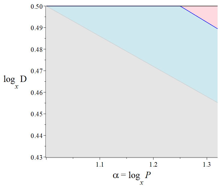
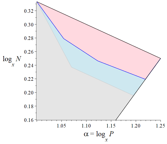
Figure 2. Type I (left) and Type II (right) ranges. Previous results in gray; our improvements in blue; conditional ranges in red (assuming Selberg’s eigenvalue conjecture).

Proposition 7.3 (Type I estimate).

For any sufficiently small $\varepsilon>0$ there exists $\delta>0$ such that the following holds. With Notation 7.2, $1\leq\alpha\leq 1.4$, $\theta:=7/32$, and $D\geq 1$, one has

$$\sum_{d\leq D}\lambda_{d}\sum_{q\equiv 0\ (\textnormal{mod }d)}\left(|\mathcal{A}_{q}|-X\frac{\rho(q)}{q}\right)\Psi\left(\frac{q}{P}\right)\log q\ll_{\varepsilon}x^{1-\delta},$$ (7.3)

for any divisor-bounded coefficients $(\lambda_{d})$, provided that

$$D\ll_{\varepsilon}x^{-\varepsilon}\min\left(x^{1/2},x^{2(1-\theta\alpha)/(4-5\theta)}\right).$$

Proof.

This is a refinement of Merikoski’s [49, Prop. 1] (which explicitated the computations in Bretèche–Drappeau’s [8, §8.4]), using our Lemma 7.1.$(ii)$ instead of [8, (8.7)]. Indeed, in the first display on [8, p. 1620], by applying 7.2 for $H\leftarrow PX^{-1+\delta}$ (for $\delta=\delta(\varepsilon)$ to be chosen shortly), $Q\leftarrow D\leq x^{1/2}$ and $M\leftarrow P/D$, we instead obtain the bound

$$R_{H}(x,P,D)$$

$$\ll_{\delta}x^{1+O(\delta)}P^{-1}DH\left(H+\sqrt{\frac{P}{D}}\left(1+H^{-\theta}D^{\theta/4}\left(\frac{P}{D}\right)^{\theta/2}\right)+\sqrt{\frac{P}{H}}\left(1+D^{-3\theta/4}\left(\frac{P}{D}\right)^{\theta/2}\right)\right)$$

$$=x^{O(\delta)}\left(\frac{PD}{x}+\sqrt{PD}\left(1+x^{\theta}P^{-\theta/2}D^{-\theta/4}\right)+\sqrt{x}D\left(1+D^{-5\theta/4}P^{\theta/2}\right)\right).$$

Here, $R_{H}(x,P,D)$ resulted from our Type I sum after putting $d$ in dyadic ranges, expanding and Fourier-completing $|\mathcal{A}_{q}|$; see [8, §8.4] and then [10, §4, 5]. Overall, this bound is acceptable in 7.3 (i.e., $\ll_{\varepsilon}x^{1-\delta}$) provided that for an absolute constant $K$, one has

$$D \ll_{\varepsilon}x^{-K\delta}\min\left(x^{2}P^{-1},x^{1/2},x^{4(1-\theta)/(2-\theta)}P^{-2(1-\theta)/(2-\theta)},x^{2/(4-5\theta)}P^{-2\theta/(4-5\theta)}\right)$$

$$=x^{-\varepsilon}\min\left(x^{2-\alpha},x^{1/2},x^{(100-50\alpha)/57},x^{(64-14\alpha)/93}\right),$$

where we picked $\delta:=\varepsilon/K$ and substituted $\theta=7/32$, $P=x^{\alpha}$. A quick numerical verification shows that for $1\leq\alpha\leq 1.4$, the first and the third term do not contribute to the minimum. ∎

Proposition 7.4 (Type II estimate).

For any sufficiently small $\varepsilon>0$ there exists $\delta>0$ such that the following holds. With Notation 7.2, $\theta:=7/32$, and $MN=P$ with $M,N\geq 1$, one has

$$\sum_{\begin{subarray}{c}m\sim M\\ n\sim N\end{subarray}}a_{m}b_{n}\left(|\mathcal{A}_{mn}|-X\frac{\rho(mn)}{mn}\right)\Psi\left(\frac{mn}{P}\right)\log(mn)\ll_{\varepsilon}x^{1-\delta},$$ (7.4)

for any divisor-bounded coefficients $(a_{m})$ and $(b_{n})$, provided that one of the following holds:

• $(b_{n})$ is supported on square-free integers, and

  $$x^{\alpha-1+\varepsilon}\ll_{\varepsilon}N\ll_{\varepsilon}x^{-\varepsilon}\max\left(x^{(2-(1+\theta)\alpha)/(3-2\theta)},x^{(2-\alpha)(1-\theta)/(3-\theta)}\right);$$ (7.5)

• $(b_{n})$ is supported on primes, and

  $$x^{\alpha-1+\varepsilon}\ll_{\varepsilon}N\ll_{\varepsilon}x^{(4-3\alpha)/3-\varepsilon}.$$ (7.6)

Remark.

The upper range in Proposition 7.4.$(ii)$, which completely removes the dependency on Selberg’s eigenvalue conjecture, wins over that in Proposition 7.3.$(i)$ only for $\alpha<136/129\approx 1.054$. As in [49], assuming Selberg’s eigenvalue conjecture, the full admissible range in part $(i)$ is $N\ll_{\varepsilon}x^{(2-\alpha)/3}$, which includes the range in part $(ii)$.

Proof of Proposition 7.4.$(ii)$, assuming $(i)$.

This is a refinement of Merikoski’s [49, Prop. 4].$(ii)$, using our Lemma 7.1.$(i)$ instead of Bretèche–Drappeau’s bound [8, (8.5)].

We briefly recall that in [49, §3], Merikoski expanded and Fourier-completed $|\mathcal{A}_{mn}|$ (resulting in a sum over $1\leq|h|\leq H:=Px^{-1+\delta}$), removed the smooth cross-conditions in $h,m,n$, and inserted the condition $(m,n)=1$ to reach Type II sums $\Sigma(M,N)$. Then they applied Cauchy–Schwarz with the sum over $n$ inside, to obtain $\Sigma(M,N)\ll M^{1/2}\,\Xi(M,N)^{1/2}$, and trivially bounded the ‘diagonal’ contribution of $n_{1}=n_{2}$ using the condition $N\gg_{\varepsilon}x^{2(\alpha-1)+\varepsilon}$. To estimate the remaining sum $\Xi_{0}(M,N)$ from the second-to-last display in [49, §3.10], we apply our bound 7.1 with $q\leftarrow n_{1}n_{2}$ and $h\leftarrow h(n_{1}-n_{2})$; with our normalization of $\theta$, this gives the refined bound

$$\Xi_{0}(M,N) \ll_{\delta}x^{O(\delta)}\sum_{\begin{subarray}{c}n_{1},n_{2}\sim N\\ (n_{1},n_{2})=1\end{subarray}}\frac{1}{H}\sum_{1\leq|h|\leq H}\left(HN+\sqrt{MN^{2}}\left(1+(n_{1}n_{2},h(n_{1}-n_{2}))^{\theta/2}N^{-3\theta/2}M^{\theta/2}\right)\right)$$

$$\ll_{\delta}x^{O(\delta)}N^{2}\left(HN+M^{1/2}N+M^{(1+\theta)/2}N^{(2-3\theta)/2}\right).$$

This results in a contribution to $\Sigma(M,N)$ of

$$\ll_{\delta}x^{O(\delta)}M^{1/2}N\left(H^{1/2}N^{1/2}+M^{1/4}N^{1/2}+M^{(1+\theta)/4}N^{(2-3\theta)/4}\right)$$

$$\ll x^{O(\delta)}\left(x^{-1/2}PN+P^{3/4}N^{3/4}+P^{(3+\theta)/4}N^{(3-4\theta)/4}\right),$$

which is acceptable (i.e., $\ll_{\varepsilon}x^{1-\delta}$) provided that for a large enough absolute constant $K$,

$$N\ll_{\varepsilon}x^{-K\delta}\min\left(x^{3/2}P^{-1},x^{4/3}P^{-1},x^{4/(3-4\theta)}P^{-(3+\theta)/(3-4\theta)}\right).$$

Trivially removing the first term, picking $\delta:=\varepsilon/K$, and substituting $P=x^{\alpha}$, this proves 7.4 in the range

$$x^{2(\alpha-1)+\varepsilon}\ll_{\varepsilon}N\ll_{\varepsilon}x^{-\varepsilon}\min\left(x^{(4-3\alpha)/3},x^{(4-(3+\theta)\alpha)/(3-4\theta)}\right),$$

when $(b_{n})$ is supported on primes. The remaining ranges to consider are

$$x^{\alpha-1+\varepsilon}\ll_{\varepsilon}N\ll_{\varepsilon}\min\left(x^{2(\alpha-1)+\varepsilon},x^{(4-3\alpha)/3-\varepsilon}\right)$$ (7.7)

and

$$\min\left(x^{\alpha-1+\varepsilon},x^{(4-(3+\theta)\alpha)/(3-4\theta)-\varepsilon}\right)\ll_{\varepsilon}N\ll_{\varepsilon}x^{(4-3\alpha)/3-\varepsilon},$$ (7.8)

both of which are (barely) covered by Proposition 7.4.$(i)$. Indeed, for 7.7, a quick numerical verification shows that

$$\min\left(2(\alpha-1),\frac{4-3\alpha}{3}\right)<\frac{2-(1+\theta)\alpha}{3-2\theta}$$

for $\theta=7/32$ and all $\alpha$, the smallest gap being $\approx 0.07$, at $a=10/9$. In 7.8, we have a nontrivial range only when

$$\frac{4-(3+\theta)\alpha}{3-4\theta}\leq\frac{4-3\alpha}{3}\qquad\iff\qquad\alpha\geq\frac{16}{15}\geq 1.066,$$

and for such $\alpha$, we have

$$\frac{4-3\alpha}{3}<\frac{2-(1+\theta)\alpha}{3-2\theta}.$$

Thus 7.4 holds in the full range from 7.6. ∎

We end this subsection by completing the proof of Proposition 7.4.

Proof of Proposition 7.4.$(i)$.

This is a refinement of Merikoski’s [49, Prop. 4].$(i)$, using Corollary 5.5 (plus Theorem 1.5) instead of Deshouillers–Iwaniec’s bound [9, Theorem 9].

We very briefly recall the relevant parts of Merikoski’s argument and the sizes of the parameters therein, pointing the reader to [49, §3] for details. In [49, §3.4], Merikoski expanded and Fourier-completed $|\mathcal{A}_{mn}|$, resulting in a sum over $1\leq|h|\leq H$ with

$$H:=Px^{-1+\delta},$$ (7.9)

as before. Then they removed the smooth cross-conditions in $h,m,n$, and separated $k=(m,n)$ to reach the type-II sums $\Sigma_{k}(M,N)$ from the first display on [49, p. 1275]; we need to bound these by $\ll_{\varepsilon}x^{1-\delta}/k$, for $\delta=\delta(\varepsilon)$ to be chosen.

In [49, §3.5], Merikoski applied Cauchy–Schwarz keeping the sums over $h,n$ inside, to obtain

$$\Sigma_{k}(M,N)\ll\left(\frac{M}{k}\right)^{1/2}\Xi_{k}(M,N)^{1/2},$$ (7.10)

and trivially bounded the contribution of $h_{2}n_{1}=h_{1}n_{2}$ to $\Xi_{k}$, using the condition $N\gg_{\varepsilon}x^{\alpha-1+\varepsilon}$; then they separated $n_{0}=(n_{1},n_{2})$ (and let $n_{i}\leftarrow n_{i}/n_{0}$). We note that considering nontrivial values of the GCD-parameters $k$ and $n_{0}$ was not necessary in the proof of Proposition 7.4.$(ii)$, since then $(b_{n})$ was supported on primes; in a first pass the reader can pretend that $k=n_{0}=1$.

In [49, §3.6], Merikoski expanded the condition $(m,n_{0}n_{1}n_{2})=1$ by Möbius inversion, resulting in a sum over $d\mid n_{0}n_{1}n_{2}$ (we switched notation from $\delta$ to $d$). Then they applied Gauss’ lemma ([49, Lemma 9]), resulting in sums $\Psi_{k}(R,S)$ of incomplete Kloosterman sums, ranging over $r,s$ of sizes

$$1\ll R,S\ll\sqrt{\frac{PN}{kn_{0}}}.$$ (7.11)

In [49, §3.7], Merikoski completed Kloosterman sums, resulting in a sum over $|t|\leq T$ with

$$T=x^{\delta}\frac{SdN^{2}}{Rn_{0}},$$ (7.12)

and trivially bounded the contribution of $t=0$. This ultimately leads to the sums of Kloosterman sums $\widetilde{\Psi}_{k}(R,S)$ from [49, p. 1279], which have a relevant level of

$$\varrho:=dk^{2}n_{0}n_{1}n_{2}\asymp\frac{dN^{2}}{n_{0}}.$$ (7.13)

Finally, in [49, §3.8], Merikoski used [10, Theorem 9] to bound the trilinear sums of Kloosterman sums

$$\mathcal{K}=\mathcal{K}(d,n_{0},n_{1},n_{2}):=\max_{\alpha\ (\textnormal{mod }\varrho)}\left|\sum_{m\sim\mathcal{M}}a_{m}\sum_{n\sim\mathcal{N}}b_{n}\sum_{(c,\varrho)=1}\Phi\left(\frac{m}{\mathcal{M}},\frac{n}{\mathcal{N}},\frac{c}{\mathcal{C}}\right)S\left(m\overline{\varrho},\pm n;c\right)\right|,$$

where $\Phi$ is a smooth function as in Corollary 5.5 with $Z=1$, $(c_{h})$ are bounded coefficients,

$$a_{m}:=e\left(-m\frac{\alpha}{\varrho}\right),\qquad\qquad b_{n}:=\sum_{\begin{subarray}{c}h_{1}\sim H_{1}\\ h_{2}\sim H_{2}\\ n=h_{1}n_{2}-h_{2}n_{1}\end{subarray}}c_{h_{1}}\overline{c_{h_{2}}},$$ (7.14)

both of which depend on the level $\varrho$,

$$\mathcal{M}\ll T,\qquad\qquad\mathcal{N}\ll\frac{HN}{kn_{0}},\qquad\qquad\mathcal{C}\ll S,$$ (7.15)

and $1/2\leq H_{2}\leq H_{1}\leq H$. We will achieve better bounds for $\mathcal{K}$ by leveraging the structure of the coefficients $(a_{m})$ and $(b_{n})$. To do so, we note that the coefficients $c_{h}$ (obtained by removing the cross-condition in $h,m,n$ on [49, p. 1274]) are smooth functions of $h$. In fact, expanding $|\mathcal{A}_{mn}|-\frac{\rho(mn)}{mn}$ via Lemma 3.1 and fixing $j,u$ up to a logarithmic loss, we can use the coefficients

$$c_{h}:=\Psi_{j}\left(\frac{|h|}{H_{j}}\right)e\left(-h\frac{ux}{P}\right),$$

from 3.4, where $1\leq 2^{j}=H_{j}\leq H=Px^{-1+\delta}$, $u\asymp 1$, and $\Psi_{j}:(\frac{1}{2},2)\to\mathbb{C}$ are compactly-supported smooth functions with bounded derivatives. In particular, through Lemma 3.1 we put $|h|$ in (smooth) dyadic ranges, and then separate into positive and negative values of $h$, all before applying Cauchy–Schwarz; so the resulting variables $h_{1},h_{2}$ are of the same size. The coefficients $(b_{n})$ from 7.14 become

$$b_{n}:=\sum_{\begin{subarray}{c}h_{1},h_{2}\in\mathbb{Z}\\ n=h_{1}n_{2}-h_{2}n_{1}\end{subarray}}c_{h_{1}}\overline{c_{h_{2}}},$$

which are in a suitable form to use Theorem 1.5 (see also 5.18), with $a=1$, $H=H_{j}$, $\alpha_{i}=\pm ux/P\ll x^{\delta}H^{-1}$, and

$$L:=\frac{N}{kn_{0}}\asymp n_{1}\asymp n_{2}.$$ (7.16)

In particular, since $\varrho\geq n_{1}n_{2}\asymp L^{2}$, the tuple $(\varrho,\mathcal{N},x,(b_{n})_{n\sim\mathcal{N}},A_{\mathcal{N}},Y_{\mathcal{N}})$ satisfies 5.3 with

$$Y_{\mathcal{N}}:=\max\left(1,\frac{\mathcal{N}H_{j}}{(H_{j}+L)Lx^{\delta}}\right)\qquad\quad\text{and}\qquad\quad A_{\mathcal{N}}:=||b_{n}\mathbbm{1}_{n\sim\mathcal{N}}||_{2}+\sqrt{\mathcal{N}}\sqrt{\frac{H_{j}}{L}+\frac{H_{j}^{2}}{L^{2}}},$$ (7.17)

where we used that $T_{\mathcal{N}/L}(\alpha_{i})\ll T_{H}(\alpha_{i})\ll 1+H|\alpha_{i}|\ll x^{\delta}$. On the other hand, by Theorem 1.4 (see also 5.17), the tuple $(\varrho,\mathcal{M},x,(a_{m})_{m\sim\mathcal{M}},A_{\mathcal{M}},Y_{\mathcal{M}})$ satisfies 5.3, with

$$Y_{\mathcal{M}}:=\sqrt{\mathcal{M}}\qquad\quad\text{and}\qquad\quad A_{\mathcal{M}}:=\sqrt{\mathcal{M}}.$$ (7.18)

By Corollary 5.5, specifically 5.28, it follows that

$$\mathcal{K}\ll_{\delta}x^{O(\delta)}\left(1+\frac{\mathcal{C}}{\sqrt{\varrho Y_{\mathcal{M}}Y_{\mathcal{N}}}}\right)^{\theta}A_{\mathcal{M}}A_{\mathcal{N}}\frac{\left(\sqrt{\varrho}\mathcal{C}+\sqrt{\mathcal{M}\mathcal{N}}+\sqrt{\mathcal{M}}\mathcal{C}\right)\left(\sqrt{\varrho}\mathcal{C}+\sqrt{\mathcal{M}\mathcal{N}}+\sqrt{\mathcal{N}}\mathcal{C}\right)}{\sqrt{\varrho}\mathcal{C}+\sqrt{\mathcal{M}\mathcal{N}}},$$

and substituting 7.18 and 7.17 gives

$$\mathcal{K}\ll_{\delta}x^{O(\delta)}\left(1+\frac{\mathcal{C}}{\sqrt{\varrho}\mathcal{M}^{1/4}\max\left(1,\sqrt{\frac{\mathcal{N}H_{j}}{(H_{j}+L)L}}\right)}\right)^{\theta}\sqrt{\mathcal{M}}\left(||b_{n}\mathbbm{1}_{n\sim\mathcal{N}}||_{2}+\sqrt{\mathcal{N}}\sqrt{\frac{H_{j}}{L}+\frac{H_{j}^{2}}{L^{2}}}\right)$$ (7.19)

$$\times\frac{\left(\sqrt{\varrho}\mathcal{C}+\sqrt{\mathcal{M}\mathcal{N}}+\sqrt{\mathcal{M}}\mathcal{C}\right)\left(\sqrt{\varrho}\mathcal{C}+\sqrt{\mathcal{M}\mathcal{N}}+\sqrt{\mathcal{N}}\mathcal{C}\right)}{\sqrt{\varrho}\mathcal{C}+\sqrt{\mathcal{M}\mathcal{N}}}.$$

Since $\mathcal{N}\ll\varrho$ (which follows from $H\ll N$), the term on the second line of 7.19 is at most $\ll\sqrt{\rho}\mathcal{C}+\sqrt{\mathcal{M}}\mathcal{C}+\sqrt{\mathcal{M}\mathcal{N}}$, as in [49, p. 1280]. The resulting bound is non-decreasing in $\mathcal{M},\mathcal{C}$, so we can plug in their upper bounds from 7.15, as well as 7.12 and 7.13 to obtain

$$\sum_{d\mid n_{0}n_{1}n_{2}}\frac{1}{TH^{2}}\mathcal{K}(d,n_{0},n_{1},n_{2})\ll_{\delta}x^{O(\delta)}\max_{d\geq 1}\frac{Rn_{0}}{SdN^{2}H^{2}}\left(1+\frac{S\min\left(1,\sqrt{\frac{(H_{j}+L)L}{\mathcal{N}H_{j}}}\right)}{\sqrt{\frac{dN^{2}}{n_{0}}}\left(\frac{SdN^{2}}{Rn_{0}}\right)^{1/4}}\right)^{\theta}$$

$$\times\sqrt{\frac{SdN^{2}}{Rn_{0}}}\left(||b_{n}\mathbbm{1}_{n\sim\mathcal{N}}||_{2}+\sqrt{\mathcal{N}}\sqrt{\frac{H_{j}}{L}+\frac{H_{j}^{2}}{L^{2}}}\right)$$

$$\times\left(\sqrt{\frac{dN^{2}}{n_{0}}}S+\sqrt{\frac{SdN^{2}}{Rn_{0}}}S+\sqrt{\frac{SdN^{2}}{Rn_{0}}\mathcal{N}}\right),$$

where none of the remaining variables have implicit dependencies on $d$. The right-hand side is seen to be non-increasing in $d$, so we can plug in $d=1$ for an upper bound. Moreover, when summing over $n_{1},n_{2}\sim L=N/(kn_{0})$, we have the same bound as in [49, bottom of p. 1280] (by [49, Lemma 7]) for the contribution of $A_{\mathcal{N}}$:

$$\sum_{n_{1},n_{2}\sim L}\left(||b_{n}\mathbbm{1}_{n\sim\mathcal{N}}||_{2}+\sqrt{\mathcal{N}}\sqrt{\frac{H_{j}}{L}+\frac{H_{j}^{2}}{L^{2}}}\right)\ll\sqrt{\mathcal{N}}\max\left(H_{j}L,H_{j}^{1/2}L^{3/2}\right).$$

The resulting bound for $\sum_{n_{1},n_{2}\sim L}\sum_{d\mid n_{0}n_{1}n_{2}}\frac{1}{TH^{2}}\mathcal{K}(d,n_{0},n_{1},n_{2})$ is non-decreasing in $\mathcal{N},H_{j}$, so we can plug in the upper bounds in $\mathcal{N}\ll HL$ and $H_{j}\ll H$ and simplify the resulting expression to obtain

$$\sum_{n_{1},n_{2}\sim L}\sum_{d\mid n_{0}n_{1}n_{2}}\frac{1}{TH^{2}}\mathcal{K}(d,n_{0},n_{1},n_{2})\ll_{\delta}x^{O(\delta)}\left(1+\frac{S^{3/4}R^{1/4}n_{0}^{3/4}}{N^{3/2}}\min\left(1,\frac{\sqrt{H+L}}{H}\right)\right)^{\theta}$$

$$\times\max\left(H^{1/2}L^{3/2},L^{2}\right)\left(\frac{\sqrt{RS}}{H}+\frac{S}{H}+\sqrt{\frac{L}{H}}\right).$$

Summing over $n_{0}$ and plugging in the bounds for $R,S,L$ from 7.11 and 7.16, we get

$$\Upsilon_{k} :=\sum_{n_{0}\ll N}\rho(n_{0})\sum_{n_{1},n_{2}\sim L}\sum_{d\mid n_{0}n_{1}n_{2}}\frac{1}{TH^{2}}\mathcal{K}(d,n_{0},n_{1},n_{2})$$

$$\ll_{\delta}x^{O(\delta)}\sum_{n_{0}\ll N}\left(1+\frac{\sqrt{PN}n_{0}^{1/4}}{\sqrt{k}N^{3/2}}\min\left(1,\frac{\sqrt{H+\frac{N}{kn_{0}}}}{H}\right)\right)^{\theta}$$

$$\times\max\left(H^{1/2}\left(\frac{N}{kn_{0}}\right)^{3/2},\left(\frac{N}{kn_{0}}\right)^{2}\right)\left(\frac{\sqrt{PN}}{\sqrt{kn_{0}}H}+\sqrt{\frac{N}{kn_{0}H}}\right).$$

Using that $H\ll N$, this further yields

$$\Upsilon_{k} \ll_{\delta}\frac{x^{O(\delta)}}{k}\sum_{n_{0}\ll N}\frac{1}{n_{0}^{2-(\theta/4)}}\left(1+\frac{\sqrt{PN}}{N^{3/2}}\min\left(1,\frac{\sqrt{N}}{H}\right)\right)^{\theta}N^{2}\left(\frac{\sqrt{PN}}{H}+\sqrt{\frac{N}{H}}\right)$$

$$\ll_{\delta}\frac{x^{O(\delta)}}{k}\left(1+\min\left(\frac{\sqrt{P}}{N},\frac{\sqrt{P}}{\sqrt{N}H}\right)\right)^{\theta}\left(\frac{\sqrt{P}N^{5/2}}{H}+\frac{N^{5/2}}{\sqrt{H}}\right).$$

Since we have $N\leq\sqrt{x}\leq\sqrt{P}$ and $\sqrt{N}H\leq x^{1/4}Px^{-1+\delta}\leq x^{1/4+3/4-1+\delta}\sqrt{P}$ for the ranges in Proposition 7.4.$(i)$, we may ignore the $1$-term in the $\theta$-factor; plugging in 7.9, we obtain

$$\Upsilon_{k}\ll_{\delta}\frac{x^{1+O(\delta)}N^{5/2}}{k\sqrt{P}}\min\left(\frac{\sqrt{P}}{N},\frac{x}{\sqrt{NP}}\right)^{\theta},$$

which improves [49, (3.7)]. In light of 7.10 and $MN=P$, this gives a contribution to $\Sigma_{k}(M,N)$ of

$$\ll_{\delta}\frac{x^{1/2+O(\delta)}}{k}P^{1/4}N^{3/4}\min\left(\frac{\sqrt{P}}{N},\frac{x}{\sqrt{NP}}\right)^{\theta/2},$$

which is acceptable (i.e., $\ll_{\varepsilon}x^{1-\delta}/k$) provided that for a large enough absolute constant $K$,

$$N\ll_{\varepsilon}x^{-K\delta}\max\left(x^{2/(3-2\theta)}P^{-(1+\theta)/(3-2\theta)},x^{2(1-\theta)/(3-\theta)}P^{-(1-\theta)/(3-\theta)}\right).$$

Choosing $\delta:=\varepsilon/K$ and substituting $P=x^{\alpha}$ completes our proof. ∎

7.3. Sieve computations

To complete the proof of Theorem 1.1, it remains to adapt the calculation in [49, §2] with our Type I and Type II information.

Notation 7.5 (Set-up for sieve computations).

Further to Notation 7.2, we follow [49, p. 1257] and let $P_{x}:=P^{+}\left(\prod_{x\leq n\leq 2x}(n^{2}+1)\right)$, then use a smooth dyadic partition of unity to split

$$S(x):=\sum_{x<p\leq P_{x}}|\mathcal{A}_{p}|\log p$$

into a sum over $x\leq P\leq P_{x}$, $P=P_{j}=2^{j}x$ of

$$S(x,P):=\sum_{p}\Psi_{j}\left(\frac{p}{P}\right),$$

up to an error of $O(x)$. Here $\Psi_{j}$ are smooth functions supported on $[1,4]$, with $\Psi_{j}^{(k)}\ll_{k}1$ for all $k\geq 0$. As in [49, p.  1257], we aim to find the greatest $\overline{\omega}$ for which

$$\sum_{\begin{subarray}{c}x\leq P\leq x^{\overline{\omega}}\\ P=2^{j}x\end{subarray}}S(x,P)\leq(1-\varepsilon)\,X\log x.$$ (7.20)

Since $S(x)=X\log x+O(x)$ (see [49, (2.1)]), this would imply the lower bound $P_{x}\geq x^{\overline{\omega}}$.

Following [49, p.  1259], given $z\geq 1$ and $u\in\mathbb{Z}_{+}$, we also let $P(z):=\prod_{\text{prime }p<z}p$ and

$$S(\mathcal{A}(P)_{u},z):=\sum_{(n,P(z))=1}|\mathcal{A}_{un}|\Psi\left(\frac{un}{P}\right)\log(un),$$

so that $S(x,P)=S(\mathcal{A}(P),2\sqrt{P})$ (where dropping the $u$ index means that $u=1$). This has a corresponding main term of

$$S(\mathcal{B}(P)_{u},z):=X\sum_{(n,P(z))=1}\frac{\rho(un)}{un}\Psi\left(\frac{un}{P}\right)\log(un),$$

sums of which can be computed via [49, Lemma 1]. Finally, the linear sieve upper bound will require the solutions $F(s),f(s)$ to the delay-differential equation system from [49, p. 1263], while the Harman sieve computations will require the Buchstab function $\omega(u)$, bounded as in [49, (2.5)].

Lemma 7.6 (Linear sieve upper bound).

For any $\varepsilon>0$ there exists $\delta>0$ such that the following holds. With $\theta:=7/32$, Notation 7.2, Notation 7.5, and $D:=x^{-\varepsilon}\min\left(x^{1/2},x^{2(1-\theta\alpha)/(4-5\theta)}\right)$, one has

$$S(\mathcal{A}(P),z)\leq(1+\delta)\,X\int\Psi\left(\frac{u}{P}\right)\frac{\alpha\log x}{e^{\gamma}\log z}F\left(\frac{\log D}{\log z}\right)\frac{du}{u},$$

for any $x^{\varepsilon}<z<D$, where $\gamma$ is the Euler–Mascheroni constant.

Proof.

This is just [49, Lemma 2] with the updated parameter $D$ from our Type I information (Proposition 7.3). ∎

Proposition 7.7 (Asymptotics for Harman sieve sums).

For any $\varepsilon>0$ there exists $\delta>0$ such that the following hold. With $\theta:=7/32$, Notation 7.2 and Notation 7.5, let

$$D:=x^{-\varepsilon}\min\left(x^{1/2},x^{2(1-\theta\alpha)/(4-5\theta)}\right),\qquad\qquad U:=Dx^{1-\alpha-\varepsilon}=:x^{\xi},$$

and $(\lambda_{u})$ be divisor-bounded coefficients. Also, let

$$\sigma_{0}:=\max\left(\frac{2-(1+\theta)\alpha}{3-2\theta},\frac{(1-\theta)(2-\alpha)}{3-\theta}\right)$$ (7.21)

be the exponent from Proposition 7.4.$(i)$.

• For $1\leq\alpha<228/203-O(\varepsilon)$ and

  $$\sigma:=\max\left(\frac{4-3\alpha}{3},\sigma_{0}\right)-\varepsilon,$$ (7.22)

  one has

  $$\sum_{u\leq U}\lambda_{u}\left(S\left(\mathcal{A}(P)_{u},x^{\sigma}\right)-S\left(\mathcal{B}(P)_{u},x^{\sigma}\right)\right)\ll_{\varepsilon}x^{1-\delta}.$$

• For $1\leq\alpha<139/114-O(\varepsilon)$ and

  $$\gamma:=\sigma_{0}-2\varepsilon,$$ (7.23)

  one has

  $$\sum_{u\leq U}\lambda_{u}\left(S\left(\mathcal{A}(P)_{u},x^{\gamma}\right)-S\left(\mathcal{B}(P)_{u},x^{\gamma}\right)\right)\ll_{\varepsilon}x^{1-\delta}.$$

Proof.

These are just [49, Propositions 3 and 4], adapted with our Type II information from Proposition 7.4; the additional term of $(4-3\alpha)/3$ from 7.22 comes from Proposition 7.4.$(ii)$. We note that the proof of [49, Proposition 3] requires

$$2(\alpha-1)<\sigma_{0}-O(\varepsilon)=\max\left(\frac{2-(1+\theta)\alpha}{3-2\theta},\frac{(1-\theta)(2-\alpha)}{3-\theta}\right)-O(\varepsilon),$$

which happens for $\alpha<228/203-O(\varepsilon)$. Similarly, the proof of [49, Proposition 4] requires

$$\alpha-1<\sigma_{0}-O(\varepsilon)=\max\left(\frac{2-(1+\theta)\alpha}{3-2\theta},\frac{(1-\theta)(2-\alpha)}{3-\theta}\right)-O(\varepsilon),$$

which happens for $\alpha<139/114-O(\varepsilon)$. ∎

We are now ready to prove our Theorem 1.1, in a very similar manner to [49, §2.6].

Proof of Theorem 1.1.

We follow the Harman sieve computations in [49, §2.4], applying Buchstab’s identity in the same ways (with adapted ranges corresponding to the values of $D,U,\sigma_{0},\sigma,\gamma,\xi$ from Lemmas 7.6 and 7.7). The five ranges relevant in the proof are now $\alpha<25/24$, $25/24\leq\alpha<228/203$, $228/203\leq\alpha<7/6$, $7/6\leq\alpha<139/114$, and $\alpha\geq 139/114$. Here, the values $228/203$ and $139/114$ come from Proposition 7.7, while $25/24$ and $7/6$ are the thresholds deciding the inequalities $\alpha<\xi+2\sigma$, respectively $2(\alpha-1)<\xi$, up to $o(1)$ factors. Indeed, we recall that

$$\xi=\min\left(\frac{1}{2},\frac{2(1-\theta\alpha)}{4-5\theta}\right)-(\alpha-1)-2\varepsilon,$$

and only the first term in the minimum is relevant for the aforementioned inequalities. We thus obtain

$$\sum_{\begin{subarray}{c}x\leq P\leq x^{139/114}\\ P=2^{j}x\end{subarray}}S(x,P)\leq\left(\frac{7}{6}-1+G_{1}+G_{2}+G_{3}+G_{4}+G_{5}-G_{6}+o(1)\right)X\log x,$$

where

$$G_{1} :=\int_{1}^{25/24}\alpha\left(\int_{\sigma}^{\alpha-2\sigma}\omega\left(\frac{\alpha}{\beta}-1\right)\frac{d\beta}{\beta^{2}}+\int_{\xi}^{\alpha/2}\omega\left(\frac{\alpha}{\beta}-1\right)\frac{d\beta}{\beta^{2}}\right)d\alpha<0.02093,$$

$$G_{2} :=\int_{25/24}^{228/203}\alpha\int_{\sigma}^{\alpha/2}\omega\left(\frac{\alpha}{\beta}-1\right)\frac{d\beta}{\beta^{2}}d\alpha<0.10528,$$

$$G_{3} :=\int_{228/203}^{7/6}\alpha\int_{\sigma_{0}}^{\alpha/2}\omega\left(\frac{\alpha}{\beta}-1\right)\frac{d\beta}{\beta^{2}}d\alpha<0.07319,$$

$$G_{4} :=\int f_{4}\left(\alpha,\vec{\beta}\right)\alpha\,\omega\left(\frac{\alpha-\beta_{1}-\beta_{2}-\beta_{3}}{\beta_{3}}\right)\frac{d\beta_{1}\,d\beta_{2}\,d\beta_{3}}{\beta_{1}\beta_{2}\beta_{3}^{2}}d\alpha<0.00163,$$

$$G_{5} :=4\int_{7/6}^{139/114}\alpha\,d\alpha<0.25116,$$

$$G_{6} :=\int_{7/6}^{139/114}\alpha\int_{\alpha-1}^{\sigma_{0}}\omega\left(\frac{\alpha}{\beta}-1\right)\frac{d\beta}{\beta^{2}}d\alpha>0.02789.$$

Here, $f_{4}$ denotes the characteristic function of the set

$$\Big{\{}\frac{228}{203}<\alpha<\frac{7}{6}, \gamma<\beta_{3}<\beta_{2}<\beta_{1}<\alpha-1,$$

$$\beta_{1}+\beta_{2},\beta_{1}+\beta_{3},\beta_{2}+\beta_{3},\beta_{1}+\beta_{2}+\beta_{3}\not\in[\alpha-1,\sigma_{0}]\Big{\}}.$$

We computed the integrals $G_{i}$ (for $i\neq 5$) by directly adapting the ranges in Merikoski’s Python 3.7 code files (see [49, p. 1268]). In the expression for $G_{5}$, we implicitly used the value $D=x^{1/2-\varepsilon}$ since $\frac{1}{2}<\frac{2(1-\theta\alpha)}{4-5\theta}$ for $\alpha\leq 139/114$, and the fact that $1<1/(2(\alpha-1))\leq 3$ for $7/6\leq\alpha\leq 139/114$. Thus

$$\sum_{\begin{subarray}{c}x\leq P\leq x^{139/114}\\ P=2^{j}x\end{subarray}}S(x,P)<0.59097\,X\log x.$$

For the remaining range $\alpha\geq 139/114$, we apply Lemma 7.6 to obtain (as in [49, (2.8)])

$$\sum_{\begin{subarray}{c}x^{139/114}\leq P\leq x^{\overline{\omega}}\\ P=2^{j}x\end{subarray}}S(x,P)\leq\left(4\int_{139/114}^{1.25}\alpha\,d\alpha+(4-5\theta)\int_{1.25}^{\overline{\omega}}\frac{\alpha}{1-\theta\alpha}d\alpha\right)X\log x,$$

where $\alpha=1.25=5/4$ is the threshold where the expression for $D$ changes (i.e., when $\frac{1}{2}=\frac{2(1-\theta\alpha)}{4-5\theta}$). We conclude that 7.20 holds (for small enough $\varepsilon$) provided that

$$(4-5\theta)\int_{1.25}^{\overline{\omega}}\frac{\alpha}{1-\theta\alpha}d\alpha<1-0.59097-4\int_{139/114}^{1.25}\alpha\,d\alpha,$$

where the right-hand side is at least $0.257406$. This inequality (barely) holds true when $\overline{\omega}=1.30008$, which proves Theorem 1.1. ∎

References

- [1] Edgar Assing, Valentin Blomer, and Junxian Li. Uniform Titchmarsh divisor problems. Advances in Mathematics, 393:108076, 2021.
- [2] Enrico Bombieri. On the large sieve. Mathematika, 12(2):201–225, 1965.
- [3] Enrico Bombieri, John B. Friedlander, and Henryk Iwaniec. Primes in arithmetic progressions to large moduli. Acta Math., 156(1):203–251, 1986.
- [4] Enrico Bombieri, John B. Friedlander, and Henryk Iwaniec. Primes in arithmetic progressions to large moduli. II. Mathematische Annalen, 277(3):361–393, 1987.
- [5] Enrico Bombieri, John B. Friedlander, and Henryk Iwaniec. Primes in arithmetic progressions to large moduli. III. Journal of the American Mathematical Society, 2(2):215–224, 1989.
- [6] Daniel Bump. Automorphic forms and representations, volume 55. Cambridge university press, 1998.
- [7] Javier Cilleruelo and Moubariz Z Garaev. Concentration of points on two and three dimensional modular hyperbolas and applications. Geometric and Functional Analysis, 21(4):892, 2011.
- [8] Régis de La Bretèche and Sary Drappeau. Niveau de répartition des polynômes quadratiques et crible majorant pour les entiers friables. Journal of the European Mathematical Society, 22(5):1577–1624, 2020.
- [9] Jean-Marc Deshouillers and Henryk Iwaniec. Kloosterman sums and fourier coefficients of cusp forms. Inventiones mathematicae, 70(2):219–288, 1982.
- [10] Jean-Marc Deshouillers and Henryk Iwaniec. On the greatest prime factor of . In Annales de l’institut Fourier, volume 32, pages 1–11, 1982.
- [11] Sary Drappeau. Théorèmes de type Fouvry–Iwaniec pour les entiers friables. Compositio Mathematica, 151(5):828–862, 2015.
- [12] Sary Drappeau. Sums of Kloosterman sums in arithmetic progressions, and the error term in the dispersion method. Proc. Lond. Math. Soc., 114(4):684–732, 2017.
- [13] Sary Drappeau, Andrew Granville, and Xuancheng Shao. Smooth-supported multiplicative functions in arithmetic progressions beyond the -barrier. Mathematika, 63(3):895–918, 2017.
- [14] Sary Drappeau, Kyle Pratt, and Maksym Radziwiłł. One-level density estimates for Dirichlet L-functions with extended support. Algebra & Number Theory, 17(4):805–830, 2023.
- [15] William Duke, John B. Friedlander, and Henryk Iwaniec. Equidistribution of roots of a quadratic congruence to prime moduli. Annals of Mathematics, 141(2):423–441, 1995.
- [16] Peter D.T.A. Elliott and Heini Halberstam. A conjecture in prime number theory. In Symposia mathematica, volume 4, pages 59–72, 1968.
- [17] Étienne Fouvry. Répartition des suites dans les progressions arithmétiques. Acta Arith., 4(41):359–382, 1982.
- [18] Étienne Fouvry. Autour du théoreme de Bombieri-Vinogradov. Acta Math., 152:219–244, 1984.
- [19] Étienne Fouvry. Sur le problème des diviseurs de Titchmarsh. J. Reine Angew. Math., 357:51–76, 1985.
- [20] Étienne Fouvry. Autour du théorème de Bombieri-Vinogradov. II. Annales scientifiques de l’École Normale Supérieure, 20(4):617–640, 1987.
- [21] Étienne Fouvry and Henryk Iwaniec. On a theorem of Bombieri–Vinogradov type. Mathematika, 27(2):135–152, 1980.
- [22] Étienne Fouvry and Henryk Iwaniec. Primes in arithmetic progressions. Acta Arith., 42(2):197–218, 1983.
- [23] Étienne Fouvry, Emmanuel Kowalski, and Philippe Michel. On the exponent of distribution of the ternary divisor function. Mathematika, 61(1):121–144, 2015.
- [24] Étienne Fouvry, Emmanuel Kowalski, and Philippe Michel. Stratification and averaging for exponential sums: bilinear forms with generalized Kloosterman sums. Annali della Scuola Normale Superiore di Pisa, Classe di Scienze, 21:1453–1530, 2020.
- [25] Étienne Fouvry and Gérald Tenenbaum. Repartition statistique des entiers sans grand facteur premier dans les progressions arithmetiques. Proc. Lond. Math. Soc., 72(3):481–514, 1996.
- [26] John B Friedlander and Henryk Iwaniec. Incomplete Kloosterman sums and a divisor problem. Annals of Mathematics, 121(2):319–344, 1985.
- [27] John B Friedlander and Henryk Iwaniec. Opera de cribro, volume 57. American Mathematical Soc., 2010.
- [28] Dorian Goldfeld. Automorphic forms and L-functions for the group , volume 99. Cambridge University Press, 2006.
- [29] Andrew Granville. Integers, without large prime factors, in arithmetic progressions, I. Acta Math., 170:255–273, 1993.
- [30] Andrew Granville. Integers, without large prime factors, in arithmetic progressions. II. Philosophical Transactions of the Royal Society of London. Series A: Physical and Engineering Sciences, 345(1676):349–362, 1993.
- [31] Glyn Harman. On values of free of large prime factors. Archiv der Mathematik, 90(3), 2008.
- [32] Adam J. Harper. Bombieri–Vinogradov and Barban–Davenport–Halberstam type theorems for smooth numbers. arXiv preprint arXiv:1208.5992, 2012.
- [33] Christopher Hooley. On the greatest prime factor of a quadratic polynomial. Acta Math., 117:281–299, 1967.
- [34] Henryk Iwaniec. A new form of the error term in the linear sieve. Acta Arithmetica, 37(1):307–320, 1980.
- [35] Henryk Iwaniec. Topics in classical automorphic forms, volume 17. American Mathematical Soc., 1997.
- [36] Henryk Iwaniec. Spectral methods of automorphic forms, volume 53. American Mathematical Society, Revista Matemática Iberoamericana (RMI …, 2021.
- [37] Henryk Iwaniec and Emmanuel Kowalski. Analytic number theory, volume 53. American Mathematical Soc., 2021.
- [38] Bryce Kerr, Igor E. Shparlinski, Xiaosheng Wu, and Ping Xi. Bounds on bilinear forms with kloosterman sums. arXiv preprint arXiv:2204.05038, 2022.
- [39] Henry Kim. Functoriality for the exterior square of and the symmetric fourth of . Journal of the American Mathematical Society, 16(1):139–183, 2003 (Appendix 1 by Ramakrishnan, Appendix 2 by Kim–Sarnak).
- [40] Emmanuel Kowalski, Philippe Michel, and Will Sawin. Bilinear forms with Kloosterman sums and applications. Annals of mathematics, 186(2):413–500, 2017.
- [41] Nikolai V. Kuznetsov. Petersson’s conjecture for cusp forms of weight zero and Linnik’s conjecture. Sums of Kloosterman sums. Matematicheskii Sbornik, 153(3):334–383, 1980.
- [42] Jared Duker Lichtman. Primes in arithmetic progressions to large moduli, and shifted primes without large prime factors. arXiv preprint arXiv:2211.09641, 2022.
- [43] Jared Duker Lichtman. Primes in arithmetic progressions to large moduli, and Goldbach beyond the square-root barrier. arXiv preprint arXiv:2309.08522, 2023.
- [44] Ju V Linnik. The dispersion method in binary additive problems. American Mathematical Society, Providence, RI, 1963.
- [45] James Maynard. Small gaps between primes. Annals of mathematics, pages 383–413, 2015.
- [46] James Maynard. Primes in arithmetic progressions to large moduli I: Fixed residue classes. Memoirs of the American Mathematical Society, to appear, 2024.
- [47] James Maynard. Primes in arithmetic progressions to large moduli II: Well-factorable estimates. Memoirs of the American Mathematical Society, to appear (explicit references to arXiv:2006.07088), 2024.
- [48] James Maynard. Primes in arithmetic progressions to large moduli III: Uniform residue classes. Memoirs of the American Mathematical Society, to appear, 2024.
- [49] Jori Merikoski. On the largest prime factor of . Journal of the European Mathematical Society, 2022.
- [50] Alexandru Pascadi. Smooth numbers in arithmetic progressions to large moduli. arXiv preprint arXiv:2304.11696, 2023.
- [51] D.H.J. Polymath. Variants of the Selberg sieve, and bounded intervals containing many primes. Research in the Mathematical sciences, 1:1–83, 2014.
- [52] Peter Sarnak. Selberg’s eigenvalue conjecture. Notices of the AMS, 42(11):1272–1277, 1995.
- [53] Atle Selberg. On the estimation of Fourier coefficients of modular forms. In Proc. Symp. Pure Math., volume 8, pages 1–15. AMS, 1965.
- [54] Igor E. Shparlinski. Character sums with smooth numbers. Archiv der Mathematik, 110(5):467–476, 2018.
- [55] Igor E. Shparlinski and Tianping Zhang. Cancellations amongst Kloosterman sums. Acta Arith., 176(3):201–210, 2016.
- [56] Berke Topacogullari. On a certain additive divisor problem. Acta Arith., 181(2):143–172, 2017.
- [57] Berke Topacogullari. The shifted convolution of generalized divisor functions. International Mathematics Research Notices, 2018(24):7681–7724, 2018.
- [58] Askold I. Vinogradov. The density hypothesis for Dirichet -series. Izv. Akad. Nauk SSSR Ser. Mat, 29:903–934, 1965.
- [59] Nigel Watt. Kloosterman sums and a mean value for Dirichlet polynomials. Journal of Number Theory, 53(1):179–210, 1995.
- [60] Ping Xi. Ternary divisor functions in arithmetic progressions to smooth moduli. Mathematika, 64(3):701–729, 2018.
- [61] Yitang Zhang. Bounded gaps between primes. Annals of Mathematics, pages 1121–1174, 2014.