A Unified Algorithmic Framework for Dynamic Assortment Optimization under MNL Choice

Shuo Sun, Rajan Udwani Department of Industrial Engineering and Operations Research, UC Berkeley, Berkeley, CA 94720, shuo_sun@berkeley.edu, udwani@berkeley.edu Zuo-Jun (Max) Shen Faculty of Engineering & Faculty of Business and Economics, University of Hong Kong, Hong Kong, maxshen@hku.hk

We consider assortment and inventory planning problems with dynamic stockout-based substitution effects and no replenishment. We consider two settings: 1. Customers can see all available products when they arrive, which is commonly seen in physical stores. 2. The seller can choose to offer a subset of available products to each customer, which is typical on online platforms. Both settings are known to be computationally challenging, and the current approximation algorithms for the two settings are quite different. We develop a unified algorithm framework under the MNL choice model for both settings. Our algorithms improve on the state-of-the-art algorithms in terms of approximation guarantee, runtime, and the ability to manage uncertainty in the total number of customers and handle more complex constraints. In the process, we establish various novel properties of dynamic assortment planning (under the MNL choice) that may be useful more broadly.

1 Introduction

Choosing the optimal assortment of products to offer and determining the inventory levels for each product are fundamental problems in various industries, including retail and airlines. There has been extensive research on static assortment optimization where an optimal assortment is selected for a single customer. This setting assumes that we can stock a sufficiently large inventory for each product so that all customers see the same assortment, which is suitable for scenarios where inventory is not a primary concern, such as for digital goods or services. However, in many real-world scenarios, inventory is finite, and the sequential arrival of customers creates dynamics where products often stock out, leading to notable sales losses in both retail and the sharing economy. Therefore, in addition to deciding which products to stock, it is necessary to consider the dynamic assortment planning problem where we decide how much each product to stock and what assortment to offer to each arriving customer. The dynamic assortment planning problem is notoriously challenging due to the dynamic stockout-based substitution behavior, where customers make purchases based on the available products. (Mahajan and Van Ryzin 2001, Aouad et al. 2018). The demand for each product can be modeled through a stochastic consumption process, which is a sequence of customer choices - upon arrival, a customer randomly selects from available products offered, and the choice probability is determined by the choice model. Thus, the demand for each product is influenced by both customer preferences and the occurrence of stockouts, with these two factors being deeply interconnected. Customer preferences can lead to earlier stockouts for more preferred products, and stockouts affect purchase probabilities since the choice probabilities depend on which products are available. In fact, even efficiently evaluating the expected revenue given a starting inventory (and assortment policy) remains challenging for many choice models, including the Multinomial Logit (MNL) model.

In this work, we consider constrained single-period dynamic assortment planning problems, focusing on developing provable approximate algorithms. Dynamic assortment optimization problems vary across operating environments. In brick-and-mortar retail, once the initial inventory decisions are made, every customer entering the store sees all the available products, and assortment changes sporadically (Aouad et al. 2018, 2019). Conversely, online platforms make it easy to provide real-time personalized assortments from available products (Bai et al. 2022). We distinguish these two settings as the dynamic assortment optimization problem (da) and dynamic assortment optimization with personalization problem (dap), respectively. The existing algorithmic approaches for da and dap are quite different. For dap, when the number of customers is known, there is a natural LP relaxation that serves as a good (fluid) approximation for the expected revenue in the stochastic consumption process. In particular, one can optimize the LP objective, leading to a considerably simpler problem while losing a constant factor in the approximation guarantee (Bai et al. 2022). However, for da, where we are not allowed to change the assortments manually, no strong fluid relaxation was known (to the best of our knowledge). Existing algorithms directly optimize the expected revenue that appears hard to evaluate exactly, which use Monte Carlo sampling to estimate objective value and use computationally intensive enumerative procedures to identify the approximate inventory solutions (Aouad et al. 2018, Aouad and Segev 2022). These challenges highlight the complexities of the da problem and the pressing need for more scalable and efficient algorithmic solutions. Additionally, this raises the intriguing question of whether a unified approximation framework could effectively solve both problems.

In many applications, the number of customers (denoted as $T$) within a given planning horizon is unknown a priori. The stochasticity in $T$ adds additional complexity. In fact, in modern e-commerce and other online platforms, $T$ is often highly uncertain and may follow a high-variance distribution (Szpektor et al. 2011, El Housni et al. 2021, Aouad and Ma 2022). While for the da problem, previous work has considered different customer distributions (Aouad et al. 2018, Aouad and Segev 2022), the existing work on dap only considers deterministic $T$ (Bai et al. 2022). Consequently, developing algorithms for dap under stochastic $T$ remains a challenging open problem.

1.1 Our Contribution

Our main contribution is to develop a unified algorithm framework that addresses both da and dap problems under the MNL choice model. Our framework offers several key advantages, including computational efficiency, improved approximation ratios, the ability to manage uncertainty in the total number of customers, and the ability to handle more complex constraints. We use a two-step approximation framework. In the first step, we develop threshold-based augmentation algorithms to approximately maximize fluid relaxations. In the second step, we make inventory and assortment decisions based on the approximate inventory solution from the first step. We develop several technical ideas to establish the new results, and some of them may be of broader interest, which will be discussed later in Section 1.2.

Table 2 compares our results with the best-known approximation ratios for dynamic assortment optimization under the MNL choice model and cardinality constraints. For da, we improve the best approximation ratio for the distributions with Increasing Failure Rate (IFR) property in Aouad et al. (2018), from $0.122-\epsilon$ to $0.194-\epsilon$. Furthermore, our approach is not randomized and is significantly faster since we avoid partial enumerations that can be time intensive (polynomial in $n^{\frac{1}{\epsilon}}$, where $n$ is the number of products) and Monte Carlo sampling (polynomial in $\frac{1}{\delta}$, where $\delta$ is the probability of failure). Specifically, our algorithm has runtime $O(n^{2}K\log_{1+\epsilon}\frac{K}{\epsilon})$, where $K$ is the cardinality constraint. Aouad and Segev (2022) give a near-optimal algorithm for DA, which is not polynomial time (see Section 1.3 for more details). In addition, for the da problem, our algorithm addresses the previously open problem of accommodating a budget constraint (Aouad et al. 2018), achieving an approximation ratio of $0.194$, the same as that for a cardinality constraint.

For dap, we achieve an approximation ratio of $\frac{1}{2}(1-\frac{1}{e})$ for deterministic $T$, surpassing the current best guarantee of $\frac{1}{4}(1-\frac{1}{e})$ (Bai et al. 2022). Perhaps more importantly, our approach extends to the setting where $T$ is uncertain and follows an arbitrary (known) distribution, including high variance distributions, where no approximation results were known previously. In such scenarios, our algorithm achieves a $(0.25-\epsilon)-$approximation.

	da	dap
Deterministic	$0.158-\epsilon\rightarrow\mathbf{0.32-\epsilon}$	$\frac{1}{4}(1-\frac{1}{e})\rightarrow\mathbf{\frac{1}{2}(1-\frac{1}{e})-\epsilon}$
IFR	$0.122-\epsilon\rightarrow\mathbf{0.194}-\epsilon$	$?\rightarrow\mathbf{0.25-\epsilon}$
General Distribution	$?$	$?\rightarrow\mathbf{0.25-\epsilon}$

Table 1: Comparison of best-known approximation ratio guarantees in relevant settings. (Entries in bold represent our results. ? indicates that no result was known prior to our work.)

1.2 Technical Ideas

We use a two-step approximation algorithmic framework. We first find approximate inventory solutions to maximize the fluid approximation of the total expected revenue given constraints. Our fluid approximations are based on the choice-based linear program (CDLP), which is a standard relaxation used in the revenue management literature. We use $f^{\text{LP}}$ and $f^{\text{LP}}_{\mathbf{M}}$ to denote the optimal CDLP objective function value considering a single customer type or multiple types, named differently due to their distinct structural properties, as we will discuss later.

Approximating the optimal inventory to the fluid relaxation. While for dap, it is known that $f^{\text{LP}}_{\mathbf{M}}$ is an effective fluid approximation for the stochastic expected revenue, for da, it is highly non-trivial to determine whether $f^{\text{LP}}$ serves as an effective relaxation. By effective relaxation, we mean that one can obtain the inventory (and assortment) solutions such that the original expected revenue is at least a constant factor of $f^{\text{LP}}$. In fact, when inventory is fixed, $f^{\text{LP}}$ can be arbitrarily larger than the expected revenue even for the MNL choice model. We show that $f^{\text{LP}}$ is an effective relaxation for da under the MNL choice model for both deterministic $T$ and stochastic $T$, which will be discussed later. So now, let us focus on approximating the optimal inventory for $f^{\text{LP}}$. It is well known that $f^{\text{LP}}$ does not exhibit submodularity even when $T=1$. Bai et al. (2022) propose a modified LP (surrogate) that gives a $\frac{1}{2}-$approximate to $f^{\text{LP}}_{\mathbf{M}}$ (multiple types) that is submodular. As a straightforward extension of their result, we show that for a single customer type, their result can be strengthened, and we obtain a submodular surrogate that is a (1-$\epsilon$)-approximation for maximizing $f^{\text{LP}}$. Our main new contribution is an improved $\frac{1}{2}$ approximation algorithm for maximizing $f^{\text{LP}}_{\mathbf{M}}$, even when $T$ comes from an arbitrary stochastic distribution. To show this, we first prove that the decreasing order of prices is a submodular order (SO) for $f^{\text{LP}}$ (single type). This gives a $\frac{1}{2}$ approximation for $f^{\text{LP}}$ using the threshold algorithm for maximizing SO functions. Perhaps surprisingly, this order is not SO for $f^{\text{LP}}_{\mathbf{M}}$ because $f^{\text{LP}}_{\mathbf{M}}$ allocations the inventory of each item between different customer types. We propose a novel threshold-based algorithm that gives a $\frac{1}{2}$- approximate solution for maximizing $f^{\text{LP}}_{\mathbf{M}}$ given a cardinality constraint and $\frac{1}{3}$ for a budget constraint. Proving that $f^{\text{LP}}$ is SO is quite challenging as the LP optimal solution may change in non-trivial ways due to small changes in inventory. We prove new structural properties of $f^{\text{LP}}$: We show $f^{\text{LP}}$ is equal to the total revenue in a fluid process that starts with an inventory vector with generalized revenue-ordered property. Moreover, we establish new structural properties to analyze the influence of changing the starting inventory on the revenue in the fluid process. The revenue-ordered structure and structural properties also inspire us to develop a near-linear time algorithm to solve $f^{\text{LP}}$. Given the widespread application of CDLP in revenue management, this fast algorithm may be of independent interest (see Appendix LABEL:app:fast_cdlp for details).

Transformation to inventory and assortment decisions. For da, when inventory is fixed, $f^{\text{LP}}$ can be arbitrarily larger than the original expected revenue, and it is unclear if we can obtain a good solution for the original problem from the approximately optimal inventory for $f^{\text{LP}}$ from the first step. This might not be surprising since $f^{\text{LP}}$ allows offering a subset of available products to each customer, while in the stochastic consumption process without personalization, low-price products may deplete late on some sample paths. This affects the purchase probability of high-price products due to the substitution effect, thus cannibalizing their demand. In dap, we can manually offer the assortment to exclude low-price products to mitigate the cannibalization effect. However, for da, this cannibalization effect generally poses a significant challenge. Perhaps surprisingly, we show that a small change to the approximate inventory for $f^{\text{LP}}$ yields a good inventory solution for da. In essence, we inductively reduce the cannibalization effect to a single ‘bad’ product and show that simple rounding of the inventory of this product can mitigate this product’s effect on overall revenue. Consequently, we obtain an inventory solution with a stochastic expected revenue of at least $(1-\frac{1}{e})(1-\frac{1}{T+1})f^{\text{LP}}$ for deterministic $T$ and $\frac{1}{e}(1-\frac{1}{\mu_{T}+1})f^{\text{LP}}$ for stochastic $T$ following an IFR distribution. Showing the $\frac{1}{e}$ for stochastic $T$ poses additional challenges, as we further use $\mu_{T}$ as a fluid approximation of $T$. We establish new stochastic inequalities to show $\frac{1}{e}$ for IFR distributions, which might be of broader interest.

In dap, once the initial inventory is decided, we use standard algorithmic ideas from online assortment to decide the real-time assortments. For deterministic $T$, we show a sampling-based approach yields $(1-\frac{1}{e})f^{\text{LP}}$, which improves over the state-of-the-art ratio of $\frac{1}{2}$ (Bai et al. 2022). When $T$ is stochastic and even follows a high-variance distribution, the online greedy algorithm achieves a performance guarantee of $\frac{1}{2}$ (Golrezaei et al. 2014). These performance guarantees hold for general choice models with weak substitutability, not just MNL.

1.3 Related Work

A significant amount of research has focused on the static assortment optimization problem. Under the MNL choice model, previous research has proposed various tractable static assortment optimization algorithms across different settings. Talluri and Van Ryzin (2004) show the optimal unconstrained assortment includes a select number of products with the highest prices, known as the revenue-order structure. Rusmevichientong et al. (2010) consider the assortment optimization problem that the number of products offered is upper bounded, proposing a polynomial algorithm for the cardinality-constrained assortment optimization problem. Other variants of this problem are also considered; for further details, see Rusmevichientong and Topaloglu (2012), Désir et al. (2014), Davis et al. (2013). For a comprehensive review of static assortment optimization under other choice models, we refer the readers to Kök et al. (2015) and Strauss et al. (2018).

The dynamic setting poses a greater challenge due to the stochastic nature of customer behavior, as customer choices depend on sample-path realizations. Several works explore the theoretical difficulty of this problem and develop heuristics based on continuous relaxation. Mahajan and Van Ryzin (2001) show the profit function for the continuous relaxation problem is not quasi-concave and propose a gradient-based heuristic to solve the continuous relaxation problem. Honhon et al. (2010) assume customers always purchase the highest-ranked available product. They use a dynamic programming formulation to model the problem and establish some structural properties to help find local maxima. Recent research has started to develop provably good approximation algorithms. Our work is most closely related to this line of work. We first review the work in da setting, i.e., we only set up a starting inventory and are not allowed to change the assortment during the selling horizon. Aouad et al. (2018) propose the first constant-factor approximation algorithm for the dynamic assortment planning problem under the MNL choice model. Then, assume that the distribution of customers satisfies the IFR property. Aouad and Segev (2022) further explore the structural properties of the stochastic consumption process under the MNL choice model and develop a Monte-Carlo algorithm to compute the starting inventory within an arbitrary degree of accuracy. The runtime is $O(\frac{1}{\delta}(nK)^{O(\frac{\log{v_{max}/v_{min}}}{\epsilon^{3}})})$, which is exponential in $\log{v_{max}/v_{min}}$, where $v_{max}$ is the maximum weight and $v_{min}$ is the minimum weight, $n$ is the number of products, and $K$ is the capacity limit on the total number of units to be stocked. Observe that this algorithm is not a polynomial-time algorithm. As such, it does not directly compare with our polynomial-time result. In addition to the work discussed previously, Goyal et al. (2016), Segev (2015), and Aouad et al. (2019) also propose approximation algorithms for dynamic assortment planning, but consider more restrictive models, such as products being consumed in a specific order. This special structure enables the use of low-dimensional dynamic programs to optimize total revenue, as noted in Aouad et al. (2018). However, the MNL model leads to an exponential number of sample paths, making dynamic programming intractable. Another line of work in dynamic assortment focuses on the setting in which the assortment offered to each customer is decided in an online manner, depending on the remaining inventory and the type of customer. The inventory may have been determined beforehand or is jointly decided with the assortment. Closely related to our work is Bai et al. (2022), which also approaches the dap problem through the lens of CDLP. However, they focus on deterministic $T$ and use an approximate LP surrogate for $f^{\text{LP}}_{\mathbf{M}}$. By showing the submodularity of the LP surrogate under the MNL choice model, they achieve a $\frac{1}{2}(1-\frac{1}{e})$ approximation for maximizing $f^{\text{LP}}_{\mathbf{M}}$, while we consider $f^{\text{LP}}_{\mathbf{M}}$ directly and develop a $\frac{1}{2}$ guarantee by generalizing algorithmic ideas for submodular order functions. They provide an overall $\frac{1}{4}(1-\frac{1}{e})$ approximate solution for the MNL choice model with deterministic $T$ and a $(1-(\sqrt{2}+1)^{3}\sqrt{\frac{n}{K}})$ approximate solution for a general choice model. We improve the approximation guarantee for MNL to $\frac{1}{2}(1-\frac{1}{e})$ for deterministic $T$ and also consider stochastic $T$, which may follow an arbitrary distribution. For further discussion of online assortment optimization problems, the reader may refer to recent work and literature reviews in Ma and Simchi-Levi (2020), Rusmevichientong et al. (2020), Ma et al. (2021), and Chen et al. (2022).

There is some other work considering joint assortment and inventory problems but focusing on developing sublinear regret guarantees. Liang et al. (2021) consider the single-period joint assortment and inventory problem under MNL choice with a non-zero existing initial inventory. They show that fluid LP relaxation can be solved by sequentially solving a series of simpler linear programs, and the optimal solutions of these LPs have the ‘quasi gain-ordered’ property. We establish a different generalized revenue-ordered property for the starting inventory of a fluid process that results in the same revenue as $f^{\text{LP}}_{\mathbf{M}}$. This coincidence suggests that the optimal inventory for different variants of dynamic assortment problems might have different revenue-ordered-like properties. Mouchtaki et al. (2021) propose a sample average approximation based algorithm for the unconstrained problem, which achieves sublinear regret under a Markov chain choice model. Guo et al. (2023) consider an unconstrained problem under general choice models and arbitrary distribution of customers and reformulate the fluid LP as a bilevel optimization problem. Additionally, some work combines learning and dynamic assortment optimization. Liang et al. (2023) study the dynamic assortment planning problem under the MNL choice with unknown preference weights, which focus on learning the weights and use an existing solution algorithm for the dynamic assortment optimization problem as an oracle.

1.4 Outline

The remainder of this paper is organized as follows. Section 2 provides the problem formulation and introduces preliminary results essential for subsequent discussions. Section 3 details the approximation algorithms for the fluid relaxations. Section 4 introduces the algorithms that transform approximate solutions into inventory and assortment decisions. Finally, section 5 analyzes the overall performance guarantees and runtime, including further algorithm acceleration techniques.

2 Preliminaries

In this section, we formulate the dap and da problems and their fluid relaxations. We also introduce some technical results that are important in our algorithmic approach and analysis.

2.1 Problem Formulations

We start with the common setup for both the dap and da problems. Let $\mathbf{N}=\{1,2,\dots,n\}$ denote the ground set of products sorted in the descending order of the (fixed) per-unit prices $r_{1}\geq r_{2}\geq\dots\geq r_{n}$. We need to decide the stocking level for each product, and we use $c_{i}$ to denote the number of units (stocking level) of product $i$. These stocking levels are collectively represented by a vector $\mathbf{c}=(c_{i})_{i\in\mathbf{N}}$. Let $\mathbf{e}_{i}\in[0,1]^{n}$ denote the unit vector that only the $i$th component is $1$ and other components are all $0$. Let $T$ denote the number of customers in the selling horizon. Alternatively, this can be viewed as a selling horizon of $T$ periods, with one customer arriving in each period. We use $t\in[T]$ to denote customer $t$ arriving in period $t$. $T$ may be known (deterministic) or unknown (stochastic) when the inventory decisions are made. For stochastic $T$, we denote its distribution by $D_{T}$, which is assumed to be known.

2.1.1 DA Problem

In the da problem, the selling horizon starts with an inventory $\mathbf{c}$. Upon arrival, customer $t$ sees all products with non-zero inventory (available products), and makes at most one purchase independently based on the MNL choice model $\phi:\mathbf{N}\times 2^{\mathbf{N}}\to[0,1]$. For the MNL model, let $v_{k}$ denote the attraction parameter for product $k$. Recall that the probability $\phi(k,S)$ in MNL choice model is given by $\phi(k,S)=\frac{v_{k}}{\sum_{i\in S}v_{i}+v_{0}}$. Here $0$ denotes the outside option and $v_{0}$ is its attraction parameter. Without loss of generality, we let $v_{0}=1$.

Our objective is to identify a feasible starting inventory $\mathbf{c}\in\mathcal{F}$ that maximizes the expected total revenue. Here $\mathcal{F}$ is the feasible region given by a cardinality constraint $\|\mathbf{c}\|_{1}\leq K$ or a budget constraint $\sum_{i\in N(\mathbf{c})}b_{i}c_{i}\leq B$ for certain values of $B$, $K$ and $(b_{i})_{i\in\mathbf{N}}$. Let $Z_{i}(\mathbf{c},T)$ denote the expected number of units of product $i$ consumed in the selling horizon with $T$ customers and starting inventory $\mathbf{c}$. Then, the total expected revenue $f(\mathbf{c},T)$ is given by

$$f(\mathbf{c},T)=\sum_{i\in\mathbf{N}}r_{i}Z_{i}(\mathbf{c},T).$$

When $T$ is stochastic, we only know the distribution of $T$, not its actual value. Thus, the objective function is

$$\mathbb{E}_{T}[f(\mathbf{c},T)]=\sum_{i\in\mathbf{N}}r_{i}\mathbb{E}_{T}[Z_{i}(\mathbf{c},T)].$$

Similar to previous work, we assume that the distribution of $T$ satisfies the IFR property for the da setting, meaning that $\frac{\mathbb{P}(T=k)}{\mathbb{P}(T\geq k)}$ is non-decreasing for any $k\in\mathbb{Z}_{+}$. This property holds for various distributions used in the literature, such as exponential, Poisson, and geometric distributions (Goyal et al. 2016, Aouad et al. 2018).

2.1.2 DAP Problem

In the dap problem, there are $m$ different types of customers, denoted by $\mathbf{M}=\{1,2,\dots,m\}$. A customer of type $k\in\mathbf{M}$ chooses (independently) according to the MNL choice model $\phi_{k}:\mathbf{N}\times 2^{\mathbf{N}}\to[0,1]$, with attraction parameters $\{v_{ki}\}_{i\in\mathbf{N}}$. The probability that customer $t$ belongs to type $k$, given by $\lambda_{k,t}$, is known in advance. Every customer’s type is independent and realized on arrival. Unlike the da problem where customers see all available products, in dap, when a customer of type $k$ arrives at time $t$, we select a subset of available products (assortment) to offer. We decide the assortment based on the purchase history of the first $t-1$ customers, the current customer’s type, and the distribution of future customer types. We continue using $Z_{i}(\mathbf{c},T)$ and $f(\mathbf{c},T)$ to denote the expected consumption of product $i$ and expected total revenue in the selling horizon with $T$ customers. Note that both $f$ and $Z$ depend on the chosen assortment policy and we will specify the policy in the contexts when we discuss them in subsequent sections.

When $T$ is deterministic, this setting aligns with Bai et al. (2022). When $T$ is stochastic, we decide the initial inventory $\mathbf{c}$ based on the distribution $D_{T}$ and the assortment policy. Then the total expected revenue is $\mathbb{E}_{T}[f(\mathbf{c},T)]$. Unlike the da case, here we will consider arbitrary distributions of $T$.

2.2 Fluid Relaxation (FR)

We define fluid relaxations (FR) as the optimization problems that maximize fluid approximations of the original expected revenue objective under some constraints. We start by defining these approximations, followed by some preliminary results instrumental to our algorithm and analysis.

We start with da under deterministic $T$. Given the starting inventory $\mathbf{c}$, we use the objective value of the CDLP, $f^{\text{LP}}(\mathbf{c},T)$, as a fluid approximation to the original expected revenue.

$$f^{\text{LP}}(\mathbf{c},T)=\max_{y(S)\geq 0,\forall S\subseteq\mathbf{N}}\left\{T\sum_{S\subseteq\mathbf{N}}y(S)R(S)\mid T\sum_{S\subseteq\mathbf{N}}y(S)\phi(i,S)\leq c_{i},\forall i\in\mathbf{N};\sum_{S\subseteq\mathbf{N}}y(S)=1\right\}.$$ (1)

$f^{\text{LP}}$ relaxes $f(\mathbf{c},T)$ in da problem in two ways: (i) Customers arrive continuously from time $0$ to $T$. The customer arriving at time $t$ consumes a deterministic infinitesimal amount $\phi(i,S(t))dt$ of product $i$ where $S(t)$ is the assortment offered at $t$. (ii) We can decide the mix of assortment offered to each customer. Gallego et al. (2015) introduce the following equivalent sales-based formulation (SBLP) under the MNL choice model. In this formulation, each $y_{i}$ represents the sales of product $i$, and $y_{0}$ denotes the number of customers making no purchases.

$$f^{\text{LP}}(\mathbf{c},T)=\max_{\mathbf{y}\in\mathbb{R}^{n+1}_{+}}\left\{\sum_{i\in\mathbf{N}}r_{i}y_{i}:\sum_{i\in\mathbf{N}}y_{i}+y_{0}=T,y_{i}\leq c_{i},y_{i}\leq y_{0}v_{i},\forall i\in\mathbf{N}\right\}.$$ (2)

$f^{\text{LP}}(\mathbf{c},T)$ is known to provide an upper bound for $f(\mathbf{c},T)$, as shown in Gallego and Phillips (2004), Liu and Van Ryzin (2008). Furthermore, $f^{\text{LP}}(\mathbf{c},T)$ is monotone in $\mathbf{c}$, since $\mathbf{c}$ appears on the right-hand side of the inequality constraints in $f^{\text{LP}}(\mathbf{c},T)$.

Equivalence between $f^{\text{LP}}$ and the fluid process without personalization. In the fluid process without personalization (fp), customers arrive continuously and make deterministic purchases but each arriving customer sees all available products. Consider a simple example with a ground set $\mathbf{N}=\{1,2\}$, where both products have inventories $c_{1}=c_{2}=2$, and $v_{1}=v_{2}=v_{0}=1$, with $T=4$. Thus, the purchase probabilities for both product $1$ and $2$ are $\frac{1}{3}$. Initially, the assortment is $\{1,2\}$. The two products are both consumed at the rate of $\frac{1}{3}$. At time $t=3$, product $1$ runs out, changing the assortment to $\{2\}$, with product $2$ remaining in stock until $T$. We use fp$(\mathbf{c},T)$ to denote both the fluid process starting from inventory $\mathbf{c}$ with $T$ customers and the total revenue in the process, and use $Z^{\text{FP}}_{i}(\mathbf{c},T)$ to denote the consumption of product $i$ in fp$(\mathbf{c},T)$.

For the MNL model, it is known that $f^{\text{LP}}(\mathbf{c},T)$ equals the revenue in the fp that starts with a subset of the inventory $\mathbf{c}$. Moreover, it is straightforward to show this subset of inventory is the optimal starting inventory for the fluid process where the inventory of each product is capped by $c_{i}$, i.e., $\max_{\mathbf{x}\preceq\mathbf{c}}\textsc{fp}(\mathbf{x},T)=f^{\text{LP}}(\mathbf{c},T)$. Moreover, we show that one can construct this optimal inventory by simply setting the inventory of product $i$ as the optimal solution to the SBLP. The proof is based on Lemma 8 and Lemma 10 in Goyal et al. (2022), with details in Appendix 7.1.

Lemma 2.1

For any inventory vector $\mathbf{c}$ and $T$ customers, $\max_{\mathbf{x}\preceq\mathbf{c}}\textsc{fp}(\mathbf{x},T)=f^{\text{LP}}(\mathbf{c},T)$. Moreover, given the optimal solution $\{y^{*}_{i}\}_{i\in\mathbf{N}\cup\{0\}}$ to the SBLP (2), let $x_{i}^{*}=y_{i}^{*}$ for all $i\in\mathbf{N}$. Then $\textsc{fp}(\mathbf{x}^{*},T)=\max_{\mathbf{x}\preceq\mathbf{c}}\textsc{fp}(\mathbf{x},T)=f^{\text{LP}}(\mathbf{c},T)$.

Next, we show there exists an optimal inventory for $\max_{\mathbf{x}\preceq\mathbf{c}}\textsc{fp}(\mathbf{x},T)$ that has a structure that we define as the generalized revenue-ordered property.

Generalized revenue-ordered property of the optimal starting inventory for the fluid continuous process. When $T=1$, $\max_{\mathbf{x}\preceq\mathbf{c}}\textsc{fp}(\mathbf{x},T)$ reduces to the unconstrained static assortment problem with a ground set $N(\mathbf{c})$, where $N(\mathbf{c})=\{i\in\mathbf{N}:c_{i}>0\}$ denotes the set of products with positive inventory in $\mathbf{c}$. For the MNL model, it is known that there exists a threshold such that products priced above this threshold are included in the optimal assortment, while those below are excluded (Talluri and Van Ryzin 2004). When $T>1$, we show the optimal starting inventory for the fluid process has a generalized revenue-ordered property: the inventory of products priced above the threshold are fully stocked, whereas those priced below are not stocked. The key distinction is that the product at the threshold price may be partially stocked.

Lemma 2.2 (Generalized revenue-ordered optimal inventory)

Let $\{y^{*}_{i}\}_{i\in\mathbf{N}\cup\{0\}}$ denote the optimal solution to sales-based CDLP. Define $i_{\tau}$ as the highest index $i$ for which $\sum_{k=1}^{i-1}\min\{c_{k},v_{k}y_{0}^{*}\}<T$. We construct an inventory vector $\mathbf{x}^{\mathbf{c}}\in\mathbb{R}^{n}$ as follows:

• For $1\leq i<i_{\tau}$, set $x_{i}^{\mathbf{c}}=c_{i}$;

• For $i>i_{\tau}$, set $x_{i}^{\mathbf{c}}=0$;

• $x_{i_{\tau}}(\mathbf{c})=T-y_{0}^{*}-\sum_{k=1}^{i_{\tau}-1}\min\{c_{k},v_{k}y_{0}^{*}\}$.

Then $\textsc{fp}(\mathbf{x}^{\mathbf{c}},T)=\max_{\mathbf{x}\preceq\mathbf{c}}\textsc{fp}(\mathbf{x},T)=f^{\text{LP}}(\mathbf{c},T)$.

To show the lemma, we use Lemma 2.1 and observe that sales-based CDLP (2) reduces to a fractional knapsack problem when the decision variable $y_{0}$ is fixed. The proof is included in Appendix 7.3. From here on, we use $\mathbf{x}^{\mathbf{c}}\in\mathbb{R}_{+}^{n}$ to represent the inventory vector with the generalized revenue-ordered property described as in the lemma. Note that technically $\mathbf{x}^{\mathbf{c}}$ also depends on $T$ but we omit the dependence on $T$ for the simplicity of notation. The generalized revenue-ordered structure is crucial for establishing the SO property for $f^{\text{LP}}$ (see Section 3) and for the transformation step for da (see Section 4).

Fluid relaxations in other settings. Next, we discuss the fluid relaxations in other settings. For the da problem with stochastic $T$ following an IFR distribution, we use $f^{\text{LP}}(\mathbf{c},\mu_{T})$ as a fluid approximation for the expected revenue. This LP also considers the fluid relaxation of randomness in $T$. One can show that $f^{\text{LP}}(\mathbf{c},\mu_{T})$ serves as an upper bound on $\mathbb{E}_{T}[f(\mathbf{c},T)]$; see Proposition 7.4 in Appendix 7.4 for details.

For dap, when $T$ is deterministic, we use the objective function value of multi-type CDLP as the fluid approximation, denoted as $f^{\text{LP}}_{\mathbf{M}}(\mathbf{c},T)$. The multi-type CDLP is a natural generalization of the single-type CDLP considering multiple customer types. A detailed formulation can be found in Appendix 7.5. Notably, $f^{\text{LP}}_{\mathbf{M}}(\mathbf{c},T)$ serves as an upper bound for the expected revenue in dap for any online assortment policy (Lemma 1 in Golrezaei et al. (2014)). When $T$ is stochastic and follows arbitrary distributions, $f^{\text{LP}}(\mathbf{c},\mu_{T})$ is a weak fluid relaxation, as the ratio between the original expected revenue and the $f^{\text{LP}}(\mathbf{c},\mu_{T})$ may approach $0$ when $T$ follows a high-variance distribution (Bai et al. 2023). Instead, we use $\mathbb{E}_{T}[f^{\text{LP}}_{\mathbf{M}}(\mathbf{c},T)]$ as the fluid approximation which takes the expectation of $f^{\text{LP}}_{\mathbf{M}}$ over $T$. In $\mathbb{E}_{T}[f^{\text{LP}}_{\mathbf{M}}(\mathbf{c},T)]$, we are not relaxing the stochasticity in $T$, but only in the choices of the customers. Since $f^{\text{LP}}_{\mathbf{M}}(\mathbf{c},T)\geq f(\mathbf{c},T)$ for any assortment policy, $\mathbb{E}_{T}[f^{\text{LP}}_{\mathbf{M}}(\mathbf{c},T)]$ provides an upper bound for $\mathbb{E}_{T}[f^{\text{LP}}(\mathbf{c},T)]$ under any assortment policy. Perhaps even more important is that $\mathbb{E}_{T}[f^{\text{LP}}(\mathbf{c},T)]$ upper bounds the revenue under the optimal offline policy that knows the full sequence of arrivals consider optimal inventory whereas Aouad and Ma (2022) and Bai et al. (2023) upper bounds the revenue under the optimal online policy.

For clarity, we summarize the objective functions of the fluid relaxations in the following table.

	da	dap
Deterministic $T$	$f^{\text{LP}}(\mathbf{c},T)$	$f^{\text{LP}}_{\mathbf{M}}(\mathbf{c},T)$
Stochastic $T$	$f^{\text{LP}}(\mathbf{c},\mu_{T})$	$\mathbb{E}_{T}[f^{\text{LP}}_{\mathbf{M}}(\mathbf{c},T)]$

Table 2: Objective Functions in Fluid Relaxations for Different Settings

2.3 Submodular Order Property

Given a ground set of elements $\mathbf{N}$ and a set function $g:2^{n}\rightarrow\mathbb{R}$, an order $\sigma$ is a (strong) submodular order if

$$g(A\cup\{i,j\})-g(A\cup\{j\})\leq g(A\cup\{i\})-g(A),\quad\forall A\subseteq\mathbf{N}\text{ and }i>r_{\sigma}(A\cup\{j\}).$$

Here $i>r_{\sigma}(A\cup\{j\})$ means $i$. is to the right of $A$ in order $\sigma$. Note SO is defined for a set function, and $f^{\text{LP}}$ can also be viewed as a set function. Consider an expanded ground set with many copies of each product $i\in\mathbf{N}$. Each $\mathbf{c}\in\mathbb{Z}_{+}^{n}$ specifies a subset $S_{c}$ of the expanded ground set, where $c_{i}$ is the number of copies of product $i$ in $S_{c}$. The order $\sigma$ is defined for all the items in the expanded ground set. Threshold-based augmentation algorithms can give a $\frac{1}{2}$-approximate solution to maximize monotone functions with SO property under a cardinality constraint and $\frac{1}{3}$ under a budget constraint. Udwani (2021) shows that the descending order of price is a strong submodular order for the revenue function of static assortment optimization (equivalent to the $f^{\text{LP}}$ when $T=1$). We extend their result to show that $f^{\text{LP}}$ with general $T$ has the SO property, as given in Theorem 3.2.

3 Fluid Relaxation Approximation

This section outlines the approximation algorithms for the fluid relaxations (fr). For da, we extend the result in Bai et al. (2022) to get a $(1-\frac{1}{e})-$approximate solution for deterministic $T$ in Section 3.1. For dap, our approximation algorithm leverages the SO property of $f^{\text{LP}}$. We first establish the SO property for $f^{\text{LP}}$ in Section 3.2 and then introduce the approximate algorithm for maximizing $f^{\text{LP}}_{\mathbf{M}}$ with deterministic $T$ in Section 3.3. In Section 3.4, we extend our results to the more general setting where $T$ is stochastic.

3.1 Approximation for DA

We start with deterministic $T$. Recall the formulation of the fluid relaxation is as follows:

$$\max_{\mathbf{c}\in\mathcal{F}}f^{\text{LP}}(\mathbf{c},T).$$ (3)

Recall that $f^{\text{LP}}(\mathbf{c},T)$ is monotone but not submodular, even for $T=1$. Bai et al. (2022) propose a modified LP formulation wherein the value of $y_{0}$ is fixed. Let $g(\mathbf{c},\bar{y}_{0}):\mathbb{R}^{n}\rightarrow\mathbb{R}$ denote the optimal objective value of the sales-based CDLP with $y_{0}$ fixed at $\bar{y}_{0}$. Bai et al. (2022) show that $g(\mathbf{c},\bar{y}_{0})$ is submodular in $\mathbf{c}$. They fix $y_{0}$ to $\frac{T}{2}$ and show the function gives a $\frac{1}{2}-$approximation of $f^{\text{LP}}$, thus achieving an overall guarantee of $\frac{1}{2}(1-\frac{1}{e})$ using standard submodular maximization algorithms. However, if we know the optimal value of $y_{0}$, we can use the submodular maximization algorithm to achieve a $(1-\frac{1}{e})$-approximate solution under a cardinality constraint or a budget constraint (Nemhauser et al. 1978, Sviridenko 2004, Badanidiyuru and Vondrák 2014). We show that one can find the near-optimal value of $y_{0}$ by trying a geometric series of values, thereby achieving $1-\frac{1}{e}-\epsilon$ performance guarantee. The algorithm details are provided in Appendix 8.1.

Theorem 3.1

Given any accuracy level $\epsilon\in(0,1)$, $\max_{\mathbf{c}\in\mathcal{F}}f^{\text{LP}}(\mathbf{c},T)$ can be approximated within a factor of $1-\frac{1}{e}-\epsilon$ in polynomial time.

Recall that for dap with deterministic $T$, we maximize $f^{\text{LP}}_{\mathbf{M}}$, where the decision variables in the LP are $\{y_{ki}\}_{k\in\mathbf{M},i\in\mathbf{N}\cup\{0\}}$. It is unclear how to accurately guess the $m$ near-optimal values for $\{y_{k0}\}_{k\in\mathbf{M}}$ to improve the approximation guarantee beyond $\frac{1}{2}(1-\frac{1}{e})$ in Bai et al. (2022). Furthermore, this idea cannot be generalized to optimize $\mathbb{E}_{T}[f^{\text{LP}}_{\mathbf{M}}(\mathbf{c},T)]$ for dap with stochastic $T$, where we need to guess $y_{0}$ for different customer types and different $T$. So we take a different algorithmic approach that develops threshold-based augmentation algorithms. First, we establish the SO property for $f^{\text{LP}}$. Leveraging the SO property, we generalize the threshold-based augmentation algorithm for SO functions to maximize $f^{\text{LP}}_{\mathbf{M}}(\mathbf{c},T)$ for deterministic $T$ and $\mathbb{E}_{T}[f^{\text{LP}}_{\mathbf{M}}(\mathbf{c},T)]$ for stochastic $T$. It is important to note that we consider the original CDLP, $f^{\text{LP}}_{\mathbf{M}}$, rather than the modified LP $g$, and we establish the SO property instead of submodularity.

3.2 Submodular Order Property of Single-type CDLP

In this section, we return to consider $f^{\text{LP}}(\mathbf{c},T)$. Recall that for $T=1$, it is known that the descending order of price is a submodular order. However, for $T>1$, proving the SO property becomes more challenging since it requires the structural results of the optimal solutions to LPs. We show that the descending order of price is still a submodular order for $T>1$, which is formally stated in the following theorem.

Theorem 3.2

For any given $T$, sorting products in descending order of price, breaking ties arbitrarily, is a strong submodular order for $f^{\text{LP}}(\mathbf{c},T)$. In other words, suppose the products have been sorted in the non-increasing order of prices:$r_{1}\geq r_{2}\geq\dots\geq r_{n}$, then for any $\mathbf{c}\in\mathbb{Z}_{+}^{n}$, $i,j\in\mathbf{N}$ such that $i\leq j$, $i\leq\min\{k\in\mathbf{N}:c_{k}>0\}$, we have $f^{\text{LP}}(\mathbf{c}+\mathbf{e}_{j}+\mathbf{e}_{i},T)-f^{\text{LP}}(\mathbf{c}+\mathbf{e}_{j},T)\leq f^{\text{LP}}(\mathbf{c}+\mathbf{e}_{i},T)-f^{\text{LP}}(\mathbf{c},T)$.

To prove the theorem, we first transform $f^{\text{LP}}$ to the revenue in a fluid process starting from inventory $\mathbf{x}^{\mathbf{c}}$, recall that $f^{\text{LP}}(\mathbf{c},T)=\textsc{fp}(\mathbf{x}^{\mathbf{c}},T)$ in Lemma 2.2. Then we analyze the structural properties of $\mathbf{x}^{\mathbf{c}}$ when $\mathbf{c}$ changes. We show that only the inventory of product $i$ (the lowest-price product) may change. Moreover, we establish a critical lemma, called the Separability Lemma, to analyze the influence of changing the inventory of product $i$ on the total revenue in fp. The lemma plays an important role in establishing SO as well as the transformation in Section 4. By separability, we mean that the total revenue from a fluid continuous process that starts with some extra units of product $i$ can be divided into two parts:the sales from the additional units of product $i$ and the total revenue from a truncated version of the original process. Recall that $Z^{\text{FP}}_{i}(\mathbf{c},T)$ denotes the consumption of product $i$ in fp$(\mathbf{c},T)$.

Lemma 3.3 (Separability)

For any inventory vector $\mathbf{c}$ and $T$ customers, consider two fluid processes $\textsc{fp}(\mathbf{c},T)$ and $\textsc{fp}(\mathbf{c}+\delta_{i}\mathbf{e}_{i},T)$. Let $\alpha_{i}$ denote the extra consumption of product $i$ in $\textsc{fp}(\mathbf{c}+\delta_{i}\mathbf{e}_{i},T)$, given by $\alpha_{i}=Z^{\text{FP}}_{i}(\mathbf{c}+\delta_{i}\mathbf{e}_{i},T)-Z^{\text{FP}}_{i}(\mathbf{c},T)$. Then the following holds:

1. For product $i$, $Z^{\text{FP}}_{i}(\mathbf{c}+\delta_{i}\mathbf{e}_{i},T)=\alpha_{i}+Z^{\text{FP}}_{i}(\mathbf{c},T-\alpha_{i})$. For every other product $j\neq i$, $Z^{\text{FP}}_{j}(\mathbf{c}+\delta_{i}\mathbf{e}_{i},T)=Z^{\text{FP}}_{j}(\mathbf{c},T-\alpha_{i})$. In other words, the process $\textsc{fp}(\mathbf{c}+\delta_{i}\mathbf{e}_{i},T)$ can be decomposed into two parts:the process $\textsc{fp}(\mathbf{c},T-\alpha_{i})$ and the consumption of product $i$ with probability $1$ during the interval $[T-\alpha_{i},T]$.

2. $\textsc{fp}(\mathbf{c}+\delta_{i}\mathbf{e}_{i},T)=\textsc{fp}(\mathbf{c},T-\alpha_{i})+\alpha_{i}r_{i}$.

We provide an example to illustrate this lemma. Consider a universe of three products with starting inventory $x_{1}=1$, $x_{2}=0$, $x_{3}=3$. Let $v_{1}=v_{2}=v_{3}=v_{0}=1$ and $T=8$. Then, in $\textsc{fp}(\mathbf{x},T)$, the initial assortment is $\{1,3\}$. By time $t=3$, product $1$ is out of stock, and the assortment changes to $\{2\}$. By $t=7$, product $3$ is also out of stock, so customers thereafter can see nothing. Now, suppose that we start with 2 additional units of product 2. The sequence of assortments is visualized in Figure 1(a). Figure 1(b) visualizes the process that consists of two parts:the original process truncated at time $T-\alpha_{2}$, followed by that product $2$ is consumed with probability $1$ during time $[T-\alpha_{2},T]$. Observe that in both Figure 1 (a) and (b), $\frac{1}{2}$ units of product $3$ remain at the end of the selling horizon, and the consumption of all products is identical in the two processes.

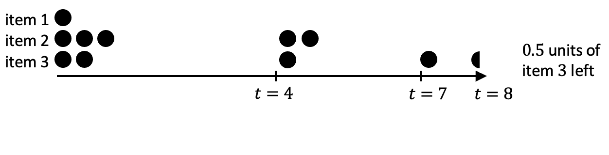
(a) $\textsc{fp}(\mathbf{c}+\delta_{i}\mathbf{e}_{i},T)$

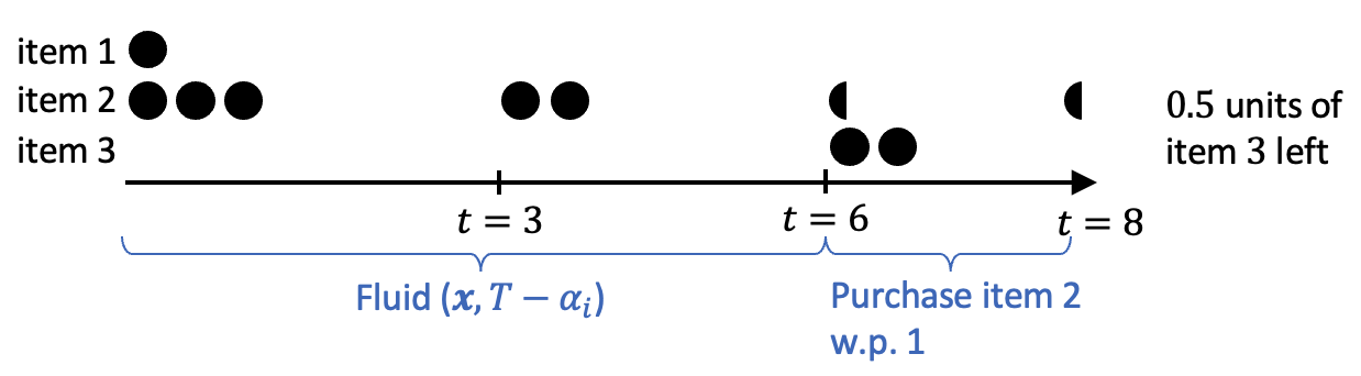
(b) Equivalence process of $\textsc{fp}(\mathbf{c}+\delta_{i}\mathbf{e}_{j},T)$

Figure 1: Example:$\textsc{fp}(\mathbf{c}+\delta_{i}\mathbf{e}_{i},T)$ and its equivalent process

The proof of this lemma relies on the Independence of Irrelevant Alternatives (IIA) property of the MNL model. A key observation is that, considering the outside option $0$ as a product that never stocks out, the purchase probability of any product $i\in\mathbf{N}$ before it runs out of stock is $\frac{v_{i}}{v_{0}}$ times the purchase probability of product $0$. Moreover, the total sales of all products, including $0$, is constantly $T$. The detailed proof is deferred to Appendix 8.2. Next, we proceed to prove Theorem 3.2.

Proof 3.4

Proof of Theorem 3.2. For clarity and brevity, we introduce the following simplified notation:Let $\mathbf{c}^{+ij}$, $\mathbf{c}^{+i}$, $\mathbf{c}^{+j}$ denote $\mathbf{c}+\mathbf{e}_{i}+\mathbf{e}_{j}$, $\mathbf{c}+\mathbf{e}_{i}$, $\mathbf{c}+\mathbf{e}_{j}$, respectively. Let $S(t)$, $S^{+i}(t)$, $S^{+j}(t)$, $S^{+ij}(t)$ denote the assortment at time $t$ in fp starting from $\mathbf{c}$, $\mathbf{c}^{+i}$, $\mathbf{c}^{+j}$, $\mathbf{c}^{+ij}$. Recall that $f^{\text{LP}}(\mathbf{c},T)=\textsc{fp}(\mathbf{x}^{\mathbf{c}},T)$ (Lemma 2.2), so it suffices to show that

$$\textsc{fp}(\mathbf{x}^{\mathbf{c}^{+ij}},T)-\textsc{fp}(\mathbf{x}^{\mathbf{c}^{+j}},T)\leq\textsc{fp}(\mathbf{x}^{\mathbf{c}^{+i}},T)-\textsc{fp}(\mathbf{x}^{\mathbf{c}},T).$$ (4)

Recall that have established the generalized revenue order property for $\mathbf{x}^{\mathbf{c}}$, which means all the inventory of products before a threshold will be included in $\mathbf{x}^{\mathbf{c}}$. The case $\textsc{fp}(\mathbf{x}^{\mathbf{c}^{+ij}},T)-\textsc{fp}(\mathbf{x}^{\mathbf{c}^{+j}},T)=0$ is trivial since the right-hand side is nonnegative due to the monotonicity of LP. We further show that when $\textsc{fp}(\mathbf{x}^{\mathbf{c}^{+ij}},T)-\textsc{fp}(\mathbf{x}^{\mathbf{c}^{+j}},T)>0$, all the available inventory of products with an index less than $i$ is included in $\mathbf{x}^{\mathbf{c}^{+ij}}$, $\mathbf{x}^{\mathbf{c}^{+j}}$, $\mathbf{x}^{\mathbf{c}^{+i}}$ and $\mathbf{x}^{\mathbf{c}}$, i.e., $x_{k}^{\mathbf{c}^{+ij}}=x_{k}^{\mathbf{c}^{+i}}=x_{k}^{\mathbf{c}^{+j}}=x_{k}^{\mathbf{c}}=c_{k}$ for all $k<i$. So we just need to consider the influence of the different number of units of product $i$.

Since both $\mathbf{x}^{\mathbf{c}^{+ij}}$ and $\mathbf{x}^{\mathbf{c}^{+j}}$ include inventory of products with an index less than $i$, from Separability Lemma, let $\alpha_{1}=Z^{\text{FP}}_{i}(\mathbf{x}^{\mathbf{c}^{+ij}})-Z^{\text{FP}}_{i}(\mathbf{x}^{\mathbf{c}^{+j}})$, we have:

$$\textsc{fp}(\mathbf{x}^{\mathbf{c}^{+ij}},T)-\textsc{fp}(\mathbf{x}^{\mathbf{c}^{+j}},T) =\alpha_{1}r_{i}+\textsc{fp}(\mathbf{c}^{+j},T-\alpha_{1}))-\textsc{fp}(\mathbf{c}^{+j},T)$$

$$={\int_{t=T-\alpha_{1}}^{T}}r_{i}-R(S^{+j}(t))dt$$ (5)

Intuitively, the marginal benefit comes from replacing the assortment in $[T-\alpha_{1},T]$ with selling product $i$ with probability $1$. We refer to $[T-\alpha_{1},T]$ as the replacement period for $\textsc{fp}(\mathbf{x}^{\mathbf{c}^{+ij}},T)$ and $\alpha_{1}$ is the length of the replacement period. We visualize the marginal benefit in Figure 2.

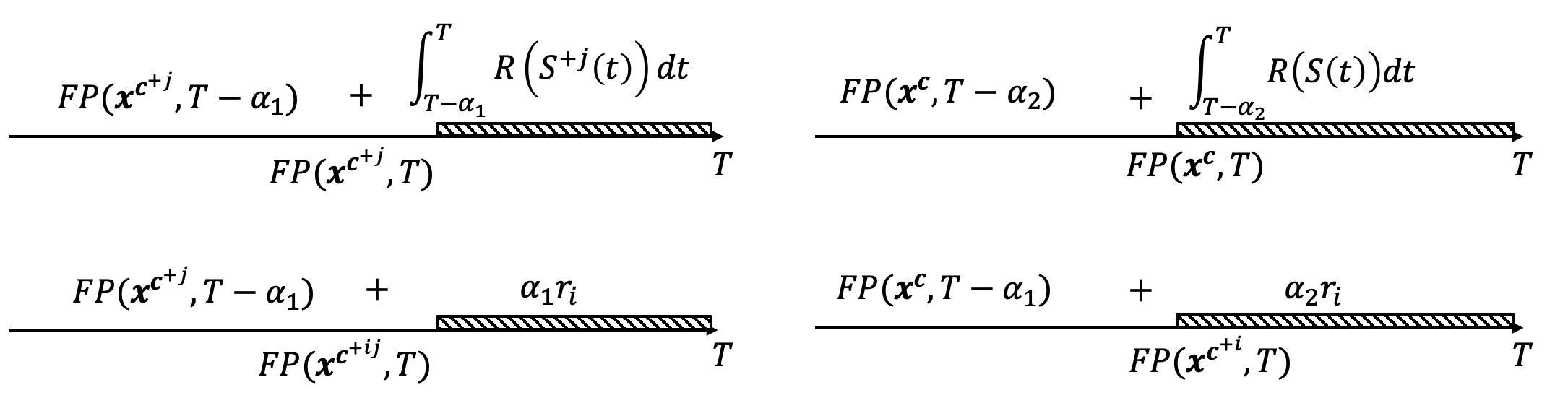
Figure 2: Left:$\textsc{fp}(\mathbf{x}^{\mathbf{c}^{+ij}})-\textsc{fp}(\mathbf{x}^{\mathbf{c}^{+j}})$. Right:$\textsc{fp}(\mathbf{x}^{\mathbf{c}^{+i}})-\textsc{fp}(\mathbf{x}^{\mathbf{c}})$

Similarly, let $\alpha_{2}=Z^{\text{FP}}_{i}(\mathbf{x}^{\mathbf{c}^{+i}})-Z^{\text{FP}}_{i}(\mathbf{x}^{\mathbf{c}})$, we have:

$$\textsc{fp}(\mathbf{x}^{\mathbf{c}^{+i}},T)-\textsc{fp}(\mathbf{x}^{\mathbf{c}},T)={\int_{t=T-\alpha_{2}}^{T}}(r_{i}-R(S(t)))dt$$ (6)

So we just need to prove $\int_{t=T-\alpha_{1}}^{T}(r_{i}-R(S^{+j}(t)))dt\leq\int_{t=T-\alpha_{2}}^{T}(r_{i}-R(S(t)))dt$, which means the total benefit from replacing the assortment by $i$ in the replacement period for $\textsc{fp}(\mathbf{x}^{\mathbf{c}^{+ij}},T)$ is lower than or equal to that in $\textsc{fp}(\mathbf{x}^{\mathbf{c}^{+i}},T)$. It suffices to show the following properties: (i) $\alpha_{1}\leq\alpha_{2}$, which means the length of replacement period for $\textsc{fp}(\mathbf{x}^{\mathbf{c}^{+i}},T)$ is at least as long as that of $\textsc{fp}(\mathbf{x}^{\mathbf{c}^{+ij}},T)$. (ii) $r_{i}-R(S(t))\geq 0$ for $t\in[T-\alpha_{1},T]$ and $r_{i}-R(S^{+j}(t))\geq 0$ for $t\in[T-\alpha_{2},T]$. This means at any time within the replacement periods for both $\mathbf{x}^{\mathbf{c}^{+i}}$ and $\mathbf{x}^{\mathbf{c}^{+ij}}$, the benefit of the replacement is non-negative. (iii) For $t\in[T-\alpha_{2},T]$, $R(S(t))\leq R(S^{+j}(t))\leq r_{i}$. At any time of the replacement period for $t$ for $\textsc{fp}(\mathbf{x}^{\mathbf{c}^{+i}},T)$, the benefit from replacing the assortment by $i$ in $\textsc{fp}(\mathbf{x}^{\mathbf{c}^{+i}},T)$ is no less than that in $\textsc{fp}(\mathbf{x}^{\mathbf{c}^{+ij}},T)$. Here (i) and (ii) are shown based on the optimality of $\mathbf{x}^{\mathbf{c}}$ for fp and the Separability Lemma. The key to showing (iii) is to observe that $S(t)\subseteq S^{+j}(t)$ due to weak substitutability, and note that $r_{i}$ has the lowest price among $N(\mathbf{c}^{+ij})$. The complete proof is provided in Appendix 8.3.

3.3 Approximation for DAP

For dap with deterministic $T$, recall we approximately solve the following fluid relaxation in the first step:

$$\max_{\mathbf{c}\in\mathcal{F}}f^{\text{LP}}_{\mathbf{M}}(\mathbf{c},T).$$ (7)

When $T=1$, $f^{\text{LP}}_{\mathbf{M}}(\mathbf{c},T)$ simplifies to the joint assortment optimization and customization problem under a mixture of MNL, which is proposed by El Housni and Topaloglu (2023). It is known that the descending order of price is a submodular order for the revenue function of this problem (Lemma 10 in Udwani (2021)). For general $T$, $f^{\text{LP}}_{\mathbf{M}}$ does not only decide the quantity of each product to use as $f^{\text{LP}}$, but also how to allocate the inventory across different customer types. Specifically, let $\{y_{ki}\}_{k\in\mathbf{M},i\in\mathbf{N}}$ denote the optimal solution to $f^{\text{LP}}_{\mathbf{M}}(\mathbf{c},T)$, then $f^{\text{LP}}_{\mathbf{M}}$ allocates $y_{ki}$ units of product $i$ to customer type $k$. Then the problem structure changes, and perhaps surprisingly, the descending order of prices is not an SO for $f^{\text{LP}}_{\mathbf{M}}$. We provide a counterexample in Appendix LABEL:app:ce-SO-multitype. This contrasts with the single-type setting, where we establish the SO property for general $T$ (Theorem 3.2). Finding other submodular orders appears to be quite challenging.

Let $f_{k}(\cdot,\cdot)$ denote the objective function of single-type CDLP under the choice model $\phi_{k}$. Inspired by the fact that $f^{\text{LP}}_{\mathbf{M}}(\mathbf{c},T)=\sum_{k\in\mathbf{M}}f^{\text{LP}}_{k}((y_{ki})_{i\in\mathbf{N}},\lambda_{k}T)$ and SO property remains closed under additivity, we consider maximizing a new function $\hat{f}(\mathbf{C},T)=\sum_{k\in\mathbf{M}}f^{\text{LP}}_{k}(\mathbf{C}_{k},\lambda_{k}T)$. We write $\hat{f}(\mathbf{C},T)$ as $\hat{f}(\mathbf{C})$ for deterministic $T$ for simplicity. Here $\mathbf{C}_{k}=(c_{ki})_{i\in\mathbf{N}}$ is the inventory allocated to customer type $k$ and $\mathbf{C}=(\mathbf{C}_{k})_{k\in\mathbf{M}}$ is the overall inventory allocation vector. So in $\hat{f}(\mathbf{C})$, the inventory allocation is not fixed by the LP but can be changed arbitrarily. The inventory allocation is called integer allocation if $\mathbf{C}$ includes only integer components and fractional allocation otherwise. Here $\mathbf{c}=\sum_{k\in\mathbf{M}}\mathbf{C}_{k}$ is the total stocking level of each product, which must satisfy the constraint $\mathbf{c}\in\mathcal{F}$. Thus, we now consider the following optimization problem:

$$\max_{\sum_{k\in\mathbf{M}}\mathbf{C}_{k}=\mathbf{c}\,,\mathbf{c}\in\mathcal{F}}\hat{f}(\mathbf{C}).$$ (8)

In the optimization problem, we decide both the quantity of each product and the amount of inventory assigned to each customer type. It is straightforward to show that (7) and (8) have the same optimal $\mathbf{c}$ and objective value. Let $\mathbf{c}^{\text{OPT}}$ and $\mathbf{C}^{\text{OPT}}$ denote the optimal solutions to (8).

When $\mathbf{C}$ is constrained to have integer components, every customer is assigned integer units of every product. We define $i_{s}$ as product $i$ exclusively offered to customer type $s$. Then the optimization problem (8) can be viewed as a subset selection problem on a larger ground set $\bar{\mathbf{N}}$ where we create $T$ copies of item $i_{s}$. As SO remains closed under additivity, the descending order of prices, breaking ties arbitrarily, is a submodular order for $\hat{f}$ on this large ground set. Recall that the threshold-based algorithm gives constant factor guarantees for maximizing monotone SO functions, where we add an item to the set if the marginal benefit exceeds a threshold $\tau$ and the value of $\tau$ depends on $\mathbf{N},\hat{f}$, $K$ and the items already in the set. We will discuss how to set $\tau$ in Appendix LABEL:app:cdlp-m-T-alg. However, $\mathbf{C}^{\text{OPT}}$ may include fractional componnets. Thus, the approximate solution we obtain by forcing $\mathbf{C}$ to be integer allocation not be a good approximation to (7). Consider a simple example where there is one single product and two customer types. Suppose the optimal solution to (8) is $\mathbf{c}^{\text{OPT}}=(1)$, $C^{\text{OPT}}_{11}=0.7$, $C^{\text{OPT}}_{21}=0.3$, which means LP assigns $0.3$ units to type $1$ and $0.7$ units to type $2$. However, If we restrict attention to integer allocationting, the marginal benefit of adding $1$ unit to either type $1$ or type $2$ may fall below $\tau$, resulting in no items being added to the inventory. We solve this difficulty by proposing a new threshold-based algorithm that may do the fractional allocation between different customer types. Given $\tau$, our new threshold based augmentation algorithm is described below. The algorithm for the budget-constrained problem, being similar, is given in Appendix LABEL:app:multi-budget.

1 Input: Cardinality $K$, threshold $\tau$, expanded ground set $\bar{\mathbf{N}}$, number of customers $T$;

2 Output: Inventory vector $\mathbf{c}$, inventory allocation vector $\mathbf{C}$. Initialize $\mathbf{c}=\mathbf{0}^{n}$, $\mathbf{C}=\mathbf{0}^{mn}$;

3 while $\|\mathbf{c}\|_{1}<K$ do

4      for $i\in\bar{\mathbf{N}}$ do

5           Find the optimal allocation of item $i$: $\mathbf{Z}^{*}=\arg\max_{\mathbf{Z}\in\mathbb{R}^{mn}_{+}:\sum_{k\in\mathcal{M}}Z_{k,i}=1,\sum_{k\in\mathcal{M}}Z_{k,j}=0,\forall j\not=i}\hat{f}(\mathbf{C}+\mathbf{Z})-\hat{f}(\mathbf{C})$ ;

6           if $\hat{f}(\mathbf{C}+\mathbf{Z}^{*})-\hat{f}(\mathbf{C})\geq\tau$ then

7                Add item $i$ to inventory and update allocation: $\mathbf{C}=\mathbf{C}+\mathbf{Z}^{*}$, $c_{i}=c_{i}+1$;

8               

9               

10               

Algorithm 1 Multi-type Threshold-Add for Cardinality-Constrained Optimization

Like the standard threshold-based augmentation algorithm for SO functions, now we still iterate over items in the descending order of prices. However, we now calculate the maximum marginal benefit each item can give considering fractional allocation to different customer types. In line 1 of the algorithm above, we calculate the optimal allocation of product $i$ that gives the maximum marginal benefit. Here $Z_{k,i}$ represents the number of units of product $i$ allocated to customer type $k$ and $\mathbf{Z}^{*}$ denotes the optimal allocation. If the maximum benefit exceeds $\tau$, we include one more unit product $i$ in the inventory vector $\mathbf{c}$ and also update $\mathbf{C}$ based on the optimal allocation of this item. Consider the previous example that $\mathbf{c}^{\text{OPT}}=(1)$, $C^{\text{OPT}}_{11}=0.7$, $C^{\text{OPT}}_{21}=0.3$. In this new algorithm, we first calculate this item’s optimal allocation, which is $\mathbf{Z}^{*}=(0.7,0.3)$. If $\hat{f}(\mathbf{Z}^{*})\geq\tau$, we set $\mathbf{c}=(1)$ and $\mathbf{C}=(0.7,0.3)$. When we select the right value of $\tau$, $\hat{f}(\mathbf{Z}^{*})\geq\tau$. So the new algorithm will output the optimal solution. A straightforward linear program can be used to obtain $\mathbf{Z}^{*}$, and we further show this can be done in $O(mn\log(mn))$ time in Appendix LABEL:app:acc. Note in this algorithm, we iterate over all items in the expanded ground set, which may be time-consuming when the size of the expanded ground set is large since we create $Tm$ copies of each product. We show that we just need to iterate over different products; see Section 5 for details.

The complete algorithm is given in Algorithm LABEL:alg:tau-m in Appendix LABEL:app:cdlp-m-T-alg. We show the output of this algorithm provides a $\frac{1}{2}-\epsilon$ approximation guarantee to (7) under a cardinality constraint. The proof leverages the SO property of $\hat{f}$ that allows fractional inventory of products. The SO property still holds for a fractional inventory of products since it is equivalent to the SO property on a larger expanded ground set of $nmT/\epsilon$ items. The proof can be seen in Appendix LABEL:app:prf-3-ap-m-ra-T.

Theorem 3.5

Algorithm LABEL:alg:tau-m outputs a $\frac{1}{2}-\epsilon$ approximate solution to problem 7 under a cardinality constraint.

For the budget constraint, the main difference is that we include one unit of product $i$ in the inventory when the maximum marginal benefit over all the customer types exceeds $b_{i}\tau$. The algorithm yields a $\frac{1}{3}-$approximate solution; see Appendix LABEL:app:cdlp-m-T-alg for details.

Theorem 3.6

Algorithm LABEL:alg:cdlp-multi-type-budget outputs a $\frac{1}{3}-\epsilon$ approximate solution to problem 7 under a budget constraint.

3.4 Stochastic $T$

So far, we focused on deterministic $T$. We now extend this to stochastic $T$ for both da and dap. For da, recall we aim to maximize $f^{\text{LP}}(\mathbf{c},\mu_{T})$ in the first step. Thus, simply replacing $T$ by $\mu_{T}$ in the algorithm introduced in 3.1 gives a $(1-\frac{1}{e})-$approximate solution under a cardinality constraint or budget constraint.

For dap with stochastic $T$, recall that we consider the following fluid relaxation in the first step:

$$\max_{\mathbf{c}\in\mathcal{F}}\mathbb{E}_{T}[f^{\text{LP}}_{\mathbf{M}}(\mathbf{c},T)].$$ (9)

In the expectation, each LP, $f^{\text{LP}}_{\mathbf{M}}(\mathbf{c},T)$, knows the value of $T$ and allocates inventory to different customer types accordingly. Note the allocation can vary for different $T$. The variation adds complexity to analyzing changes in the objective function when $\mathbf{c}$ changes, making it more challenging to approximate (9). However, $\mathbb{E}_{T}[\hat{f}(\mathbf{c},T)]$ still has SO property since the SO property remains closed under additivity. Thus, similar to deterministic $T$, we manually allocate fractional inventory for different customer types and different $T$ in the algorithm but keep the inventory vector integer-valued. More specifically, we define and maintain an inventory matrix $\mathbf{C}^{T}\in\mathbb{R}^{mn}$ for each possible value of $T$, denoted by $\{\mathbf{C}^{T}\}_{T=1}^{T_{max}}$. Here $T_{max}$ is the maximum $T$ in the support of the distribution of $T$. In the algorithm, when examining each product $i$, the difference compared with deterministic $T$ is that we first calculate the optimal allocation for each $T$ through $\mathbf{Z}^{*,T}=\arg\max_{\mathbf{Z}\in\mathbb{R}^{mn}_{+}:\sum_{k\in\mathcal{M},j\in\mathcal{N}}Z_{k,j}=1}\hat{f}(\mathbf{C}^{T}+\mathbf{Z},T)-\hat{f}(\mathbf{C}^{T},T)$. Then we calculate the expectation of the maximum marginal benefit over $T$, given by $\mathbb{E}_{T}[\hat{f}(\mathbf{C}^{T}+\mathbf{Z}^{*,T},T)-\mathbb{E}_{T}[\hat{f}(\mathbf{C}^{T},T)]$. If the expected benefit exceeds the threshold $\tau$, we add product $i$ to the inventory and update $\mathbf{C}^{T}$ for all $T$. We provide the complete Threshold Add algorithm in Appendix LABEL:app:m-car-stoch-T.

Remark 3.7

We assume we can calculate the expectation of $\hat{f}$ for high variance distributions of $T$. This is a standard assumption as in Bai et al. (2023) and Aouad and Ma (2022).

To choose the right value of $\tau$, we still try a geometric series of values. We show this algorithm provides a $(\frac{1}{2}-\epsilon)$ approximate guarantee under a cardinality constraint. The complete algorithm (Algorithm LABEL:alg:tau-m-DT) and the proof are deferred to Appendix LABEL:app:multi-budget.

Theorem 3.8

Algorithm LABEL:alg:tau-m-DT outputs a $\frac{1}{2}-\epsilon$ approximate solution to problem 9 under a cardinality constraint.

For the budget constraint, we add an item $i$ to the inventory if the expected maximum marginal benefit of adding item $i$ exceeds $b_{i}\tau$. The complete algorithm, referred to as Algorithm LABEL:alg:tau-m-DT-budget, is presented in Appendix LABEL:app:multi-stochT. The output of this algorithm provides a $\frac{1}{3}-$approximate solution.

Theorem 3.9

Algorithm LABEL:alg:tau-m-DT-budget outputs a $\frac{1}{3}-\epsilon$ approximate solution to problem 9 under a budget constraint.

4 Transformation

So far, we have identified a feasible inventory solution that is a constant factor approximation to the fluid optimization problem. We now transform it into a constant factor approximation for the original da and dap problem.

Preliminary Case of a Single Item. To understand the gap between da/dap and fr, we start by considering a simple setting with only one product $i$ of inventory $c_{i}$, and a single customer type. In da, product $i$ is displayed to each customer until the stock is depleted or time runs out, with each customer having a uniform probability $p$ of purchasing a unit. Obviously, the optimal online assortment policy in dap will also display it to each customer. Thus, the consumption of product $i$ in da and dap are the same. In fr, each customer purchases $p$ units in a deterministic fashion until $i$ stocks out. When $T$ is deterministic, the difference arises only due to the stochasticity of customer choices. Let $Z_{i}(p,T,c_{i})$ denote the expected consumption of product $i$ in a stochastic consumption process with uniform purchase probability $p$, $T$ customers, and inventory $c_{i}$. In fr, the consumption is $\min\{pT,c_{i}\}$. One can show that $Z_{i}(p,T,c_{i})\geq(1-\frac{1}{e})\min\{pT,c_{i}\}$, using standard results in the literature on online resource allocation.

Lemma 4.1 (Lemma 5.3 in Alaei et al. (2012))

Given any inventory vector $\mathbf{c}\in\mathbb{Z}_{+}^{n}$, a product $i\in\mathbf{N}$ with a uniform purchase probability $p$, and number of customers $T$, it holds that $Z_{i}(p,T,c_{i})\geq(1-\frac{1}{e})\min\{pT,c_{i}\}$.

When $T$ is stochastic, the expected consumption in fr for dap is $\mathbb{E}[\min\{Tp,c_{i}\}]$. Taking expectation over $T$ on both sides of the inequality in the above lemma, we have $\mathbb{E}[Z_{i}(p,T,c_{i})]\geq(1-\frac{1}{e})\mathbb{E}[\min\{pT,c_{i}\}]$. For da, the consumption in fr is $\min\{\mu_{T}p,c_{i}\}$ because we consider a fluid relaxation of the uncertainty in T as well as customer choice. It is straightforward to show $\mathbb{E}_{T}[Z_{i}(p,T,c_{i})]\geq\frac{1}{2}\min\{\mu_{T}p,c_{i}\}$, using results in Aouad et al. (2018) when $T$ follows an IFR distribution. We show this $\frac{1}{2}$ bound is tight when $T$ follows a geometric distribution, as seen in Appendix LABEL:app:geo-12. For non-IFR distributions, we show the gap can be arbitrarily large and provide an example in Appendix LABEL:app:exm-nonIFR.

Lemma 4.2 (Lemma 11 in Aouad et al. (2018))

Given any inventory vector $\mathbf{c}\in\mathbb{Z}^{n}$, a product $i\in\mathbf{N}$ with a uniform purchase probability $p$, and assuming $T$ follows an IFR distribution with mean $\mu_{T}$, then it holds that $\mathbb{E}_{T}[Z_{i}(p,T,c_{i})]\geq\frac{1}{2}\min\{p\mu_{T},c_{i}\}$.

Challenges with multiple items. When the inventory includes multiple items, bounding the gap between the total expected revenue in da/dap and fr seems to be more challenging. This is mainly due to the dynamic cannibalization effect, which means on some sample paths over customer choice, the low-priced products may not stock out in da/dap after they have sold out in fr. This leads to a lower purchase probability for higher-priced products than fr. In dap, we can easily mitigate this cannibalization effect by not showing the low-price products. However, in da, we are not allowed to change the assortments manually. Thus, the gap between the revenue in da and fr can be arbitrarily large, even for the MNL model. Consider a simple example where there is a single customer and two products, $\mathbf{c}=(1,1)$, $r_{1}=1$, $r_{2}=M$, $v_{1}=M$, $v_{2}=v_{0}=1$. The LP will only include product $2$ in stock, so $f^{\text{LP}}(\mathbf{c},1)=\frac{M}{2}$. However, the expected revenue in $DA$ that starts from $\mathbf{c}$ is $\frac{2M}{M+2}$ since both products are included in $\mathbf{c}$. Thus, $\frac{f(\mathbf{c},1)}{f^{\text{LP}}(\mathbf{c},1)}=\frac{4}{M+2}$, which approaches zero as $M$ tends to infinity. Therefore, even if we obtain the approximately optimal inventory for $f^{\text{LP}}$, it may not be a good inventory vector for the original problem. We show that the cannibalization effect can be reduced to a single item for a single item, and simply rounding the inventory of this item gives a good inventory solution for da for MNL choice model. For general choice models, however, the inventory vector constructed in this is arbitrarily bad for da, as we will discuss later.

4.1 Assortment policy in DAP problem

In this section, we present the online assortment personalization policy for dap. As previously discussed, in dap, we are allowed to select a subset of available products for each arriving customer, which mitigates the cannibalization effect. Note that the algorithms and performance guarantees discussed herein are not confined to MNL models but work for any choice model with weak substitutability.

4.1.1 Deterministic $T$.

For deterministic $T$, we use independent sampling and rounding algorithm and show that the expected revenue under this policy is at least $(1-\frac{1}{e})f^{\text{LP}}_{\mathbf{M}}(\mathbf{c},T)$. Although this algorithm is the same as the algorithm in Bai et al. (2022), we improve the guarantee from $\frac{1}{2}$ to $1-\frac{1}{e}$.

1 Solve the multi-type CDLP and let $\{y_{k}(S)\}_{k\in\mathbf{M},S\subseteq\mathbf{N}}$ denote an optimal solution;

2 For each time $t\in[T]$, when a type $k$ customer arrives, sample an assortment $S_{t}$ from the distribution where $\mathbb{P}(S_{t}=S)=y_{k}(S)$ for all subsets $S\subseteq\mathbf{N}$;

Show assortment $S_{t}\cap N_{t}$, where $N_{t}$ is the set of available products at time $t$.

Algorithm 2 Assortment policy for deterministic $T$

Theorem 4.3

Given any $\mathbf{c}\in\mathbb{Z}_{+}^{n}$, number of customers $T$ and any choice model with weak substitutability, let $f(\mathbf{c},T)$ denote the total expected revenue obtained by the assortment policy above, then $f(\mathbf{c},T)\geq(1-\frac{1}{e})f^{\text{LP}}_{\mathbf{M}}(\mathbf{c},T)$.

The idea of our proof is to show that when each customer arrives, the expected purchase probability of any product in $f(\mathbf{c},T)$ is no less than that in $f^{\text{LP}}_{\mathbf{M}}(\mathbf{c},T)$. Then we can use the single-product result (Lemma 4.1) to obtain $1-\frac{1}{e}$. The proof only uses the weak substitutability property and is included in Appendix LABEL:app:thm-tran-d.

4.1.2 Stochastic $T$.

For stochastic $T$, we use the online greedy policy, i.e., provide the subset of the available products with the highest revenue to each arriving customer. It is known that the online greedy algorithm yields a guarantee of $\frac{1}{2}f^{\text{LP}}_{\mathbf{M}}(\mathbf{c}^{1},T)$ without any prior knowledge of $T$ (Golrezaei et al. 2014). Consequently, the online greedy algorithm gives a $\frac{1}{2}-$performance guarantee against $\mathbb{E}_{T}[f^{\text{LP}}_{\mathbf{M}}(\mathbf{c},T)]$, even for arbitrary distributions of $T$.

At time $t$, when a type $k$ customer arrives, offer the static optimal assortment $S_{t}=\arg\max_{S\subseteq N_{t}}\sum_{i\in S}r_{i}\phi_{k}(i,S)$.

Algorithm 3 Online greedy policy for stochastic $T$

Theorem 4.4 (Corollary 1 in Golrezaei et al. (2014))

Given any $\mathbf{c}\in\mathbb{Z}_{+}^{n}$ and distribution of $T$, let $\mathbb{E}_{T}[f(\mathbf{c},T)]$ denote the expected revenue obtained by the online greedy algorithm given inventory $\mathbf{c}$, then we have $\mathbb{E}_{T}[f(\mathbf{c},T)]\geq\frac{1}{2}\mathbb{E}_{T}[f^{M}_{LP}(\mathbf{c},T)]$.

4.2 Transformation for the DA Problem

In this section, we show how to construct an inventory vector $\mathbf{c}^{DA}\in\mathbb{Z}_{+}^{n}$ given an approximate solution $\mathbf{c}$ to fr from the first step, such that the expected revenue in da can be lower bounded by a constant factor of fr.

4.2.1 Deterministic $T$ - No ‘bad’ products.

We have shown that under the MNL choice model, the exepcted revenue from the LP ($f^{\text{LP}}(\mathbf{c},T)$) is equivalent to the revenue in the fluid process starting with an inventory with generalized revenue-ordered property ($\textsc{fp}(\mathbf{x}^{\mathbf{c}},T)$). We start by considering the case that $\mathbf{x}^{\mathbf{c}}$ is an integer-valued vector and and show that setting the staring inventory to $\mathbf{x}^{\mathbf{c}}$ gives an expected revenue of at least $(1-\frac{1}{e})\textsc{fp}(\mathbf{x}^{\mathbf{c}},T)$. However, when $\mathbf{x}^{\mathbf{c}}$ includes the fractional inventory of some product, these fractional parts can significantly impact the revenue in the fluid process. So we refer to the products with fractional inventory ‘bad’ products. Fortunately, due to our construction of $\mathbf{x}^{\mathbf{c}}$, there can be at most one product with fractional inventory and we show the influence of the fractional item can be bounded for MNL model. We will discuss how to handle this ‘bad’ product later.

To show $f(\mathbf{x}^{\mathbf{c}},T)\geq(1-\frac{1}{e})\textsc{fp}(\mathbf{x}^{\mathbf{c}},T)$, it suffices to show the following lemma. Note the results hold for all integer inventory vectors.

Lemma 4.5

Given any inventory vector $\mathbf{x}\in\mathbb{Z}_{+}^{n}$ and product $i\in\mathbf{N}$, $Z_{i}(\mathbf{x},T)\geq(1-\frac{1}{e})Z^{\text{FP}}_{i}(\mathbf{x},T)$.

We provide a proof sketch for a simple setting with two products, with inventory $x_{1}$ and $x_{2}$. The complete proof for the general setting is given in Appendix LABEL:app:prf-thm-pro. There are two possible cases in fp: (1) Both products are available until $T$. In this scenario, for each product, the purchase probability in the stochastic process at every moment can only be higher than that in fp, so we can apply the single-item result (4.1) to obtain a $1-\frac{1}{e}$. (2) One product stocks out earlier. Without loss of generality, we consider the case that product 2 stocks out earlier than 1, at time $T_{0}$. For product 2, we have the same situation as case 1. For product $1$, however, the purchase probability at time $t>T_{0}$ in the stochastic consumption process may be lower than that in fp because product $2$ may not be depleted at $t$ in the stochastic process. If product $1$ has a high price and product $2$ has a low price, this brings the possibility of low revenue in the stochastic process. In fact, the revenue in the stochastic process is generally much lower than that in fp for the non-MNL choice model; see an example in Appendix LABEL:app:4-1. However, we show the $1-\frac{1}{e}$ result still holds for the MNL choice model by transforming $Z^{\text{FP}}(\mathbf{x},T)$ and $Z(\mathbf{x},T)$ into the consumption in two processes with uniform purchase probabilities: For the stochastic consumption process, if at some time $t<T_{0}$, product $2$ is not chosen, then conditioned on this, the probability that $1$ is chosen is $\phi(1,\{1\})$, which is the probability that $1$ is chosen when only $1$ is available. Since there are at most $c_{2}$ customers who could have chosen product $2$ before $t$, we can lower bound $Z_{1}(\mathbf{x},T)$ by the expected consumption in a stochastic process with $c_{2}$ units of product $2$ and $T-c_{2}$ customers. We have $Z_{1}(\mathbf{x},T)\geq Z_{1}(x_{1}\mathbf{e}_{1},T-c_{2})$. Next, we consider the consumption in fp. Using Separability Lemma, the consumption of $1$ is equal to a process that starts with $c_{1}$ units of $1$ with length $T-c_{2}$. Now we can apply the single-product result to obtain $1-\frac{1}{e}$.

4.2.2 Stochastic $T$ - No ‘bad’ item.

Then we consider a more general setting where $T$ follows an IFR distribution. Recall that in this setting, we consider a fluid relaxation of $T$ and use $f^{\text{LP}}(\mathbf{c},\mu_{T})$ as fr. We still focus on the scenario that $\mathbf{x}^{\mathbf{c}}$ is an integer-valued factor. Establishing the performance guarantee for the original expected revenue is more challenging since $f^{\text{LP}}(\mathbf{x},\mu_{T})$ further considers fluid relaxation of $T$ while $\mathbb{E}_{T}[Z_{i}(\mathbf{x},T)]$ considers different $T$. We establish novel stochastic inequalities to show a $\frac{1}{e}$ approximation factor. The $\frac{1}{e}$ ratio frequently appears in the pricing literature considering IFR distributions (Dhangwatnotai et al. 2010, Chen et al. 2021). To the best of our knowledge, this is a mere coincidence, as the ratio we analyze involves substantially different quantities.

Lemma 4.6

Consider any inventory vector $\mathbf{x}\in\mathbb{Z}_{+}^{n}$, for any product $i\in\mathbf{N}$, then $\mathbb{E}_{T}[Z_{i}(\mathbf{x},T)]\geq\frac{1}{e}Z^{\text{FP}}_{i}(\mathbf{x},\mu_{T})$.

We continue providing a proof sketch with a simple setting with two products, with the complete proof in Appendix LABEL:app:prf-lem-IFRe. Considering the fluid process $\textsc{fp}(\mathbf{x},\mu_{T})$, there are two possibilities: (1) Both products are available until $\mu_{T}$. In this case, we can use the single-product result (Lemma 4.2) to obtain the $\frac{1}{2}$ bound. (2) Some product stocks out before $\mu_{T}$. Without loss of generality, we consider the case that product $2$ depletes before $1$, at time $T_{0}<\mu_{T}$. Recall that when $T$ is deterministic, we lower bound the consumption in da by that in a stochastic process of length $T-x_{2}$. However, now $T$ is stochastic and could be lower than $x_{2}$. To address this, we only consider $T$ greater than $x_{2}$. Formally, we have $\mathbb{E}_{T}[Z_{1}(\mathbf{x},T)]\geq\mathbb{E}_{T}[Z_{1}(x_{1}\mathbf{e}_{1},T-x_{2})\mathbbm{1}\{T>x_{2}\}]$. For the consumption in $\textsc{fp}(\mathbf{c},\mu_{T})$, we again use Separability Lemma to obtain that it is equal to the consumption in fp with length $T-x_{2}$ and only product $1$. Thus, it suffices to show $\mathbb{E}_{T}[Z_{1}(x_{1}\mathbf{e}_{1},T-x_{2})\mathbbm{1}\{T>x_{2}\}]\geq\frac{1}{e}Z^{\text{FP}}_{1}(x_{1}\mathbf{e}_{1},T-x_{2})$. However, the previous single-product bound (Lemma 4.2) cannot be directly applied since we only consider $T>x_{2}$ on the left-hand side. Our key technical contribution in this part is to establish this $\frac{1}{e}-$performance guarantee. We show it suffices to establish the $\frac{1}{e}$ ratio for the setting with one product and one unit. Recall that $Z_{i}(p,T,c_{i})$ denotes the expected consumption of product $i$ in a stochastic consumption process with uniform purchase probability $p$ of length $T$ and $c_{u}$ units in stock:

Lemma 4.7

Consider any product $i\in\mathbf{N}$ with a uniform purchase probability $p$. If $T$ follows an IFR distribution and for any integer $a<\mu_{T}$, suppose $(\mu_{T}-a)p\leq 1$, then $\mathbb{E}_{T}[Z_{i}(p,T-a,1)\mathbbm{1}\{T>a\}]\geq\frac{1}{e}p(\mu_{T}-a)$.

Establishing this lemma is technically involved and may provide insight into other revenue management problems considering IFR distributions. Here, we introduce the high-level idea of our proof and include the complete proof in Appendix LABEL:app:IFRe-2. We formulate a factor-revealing program and show $\frac{1}{e}$ is a lower bound for the program. For any $T$, $a$, $Z_{i}(p,T-a,1)=1-(1-p)^{T-a}$. Let $q_{k}=\mathbb{P}(T\geq k|T\geq k-1)$, for $i=1,2,3,\dots$; then $\mathbf{q}=(q_{1},q_{2},\dots)$ uniquely characterizes $D_{T}$. Since $D_{T}$ is an IFR distribution, it follows that $1\geq q_{1}\geq q_{2}\geq q_{3}\geq\dots\geq 0$. We can rewrite $\mathbb{P}(T\geq a)=\prod_{ik1}^{a}q_{i}$ and $Z_{k}(p,T-a)=1-(1-p)^{T-a}$. Then Lemma 4.6 is equivalent to show $\frac{1}{e}$ is a lower bound for the following factor-revealing program.

$$\min_{\mu_{T},a,p,q}\frac{q_{1}q_{2}\cdots q_{a}\mathbb{E}_{T}[(1-(1-p)^{T-a})|T\geq a]}{(\mu_{T}-a)p}$$ (10)

$$\text{s.t.}\quad 1\geq q_{1}\geq q_{2}\geq\dots\geq 0,(\mu_{T}-a)p\leq 1,0<p<1,\mu_{T}-a>0,a\in\mathbb{Z}^{+}$$

$$\quad\quad\mu_{T}=q_{1}+q_{1}q_{2}+\dots+q_{1}q_{2}\dots q_{a}(1+q_{a+1}+q_{a+1}q_{a+2}+\dots)$$

The second line delineates feasible values $a$ and $p$. The last constraint derives from the tail-sum formula for expectation. We show $\frac{1}{e}$ is a lower bound for this program through three steps: (1) we simplify the program by showing the optimal solution must have a constant value for $q_{i}$ for all $i$ beyond a certain index $k$, implying that $T-a$ conditioned on $T>a$ follows a geometric distribution. (2) we identify the structure of the optimal distribution $D_{T}$, referred to as ‘shited geometric distribution’. (3) we show the optimal objective value of the program is $\frac{1}{e}$ when restricted to shifted geometric distributions. Here we discuss the second step, which is the most challenging part. The details of other steps are technically involved and deferred to LABEL:app:prf-lem-IFRe. We identify the structure of the optimal distribution as follows.

Lemma 4.8

Given any feasible $\mu_{T}$ and $a$ with respect to (10), let $\mathbf{q}^{*}$ denote the optimal distribution to (10). Then $\mathbf{q}^{*}$ has the following structure: There exists some constant $b\in(0,1)$ with either a threshold index $1\leq k\leq a$ exists such that $q_{i}=1$ for all $i\leq k$ and $q_{i}=b$ for $i\geq k+1$, or $q_{i}=b$ for all $k\geq 1$.

Note that a standard geometric distribution has $q_{i}=b$ for all $i$ and some constant $b$. If we set $T^{\prime}=T+k$, then the distribution of $T^{\prime}$ satisfies $q_{i}=1$ for all $i\leq k$ and $q_{i}=b$ for $i\geq k+1$. Therefore, we refer to the distributions in the lemma as shifted geometric distributions. To describe the high-level idea of proving this lemma, we define the concept of a step. A step occurs if, for any $0\leq k\leq a-1$, $q_{k-1}>q_{k}>q_{k+1}$ (or $q_{a-1}>q_{a}>b$). For analytical convenience, we define $q_{0}=1$. Then, a sequence $\mathbf{q}$ having exactly $1$ step characterizes a shifted geometric distribution. In the following, we use figures to illustrate the distributions with varying numbers of steps.

(a) 1 step (Geometric distribution)

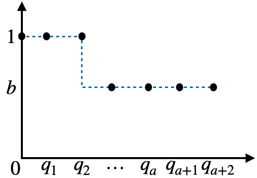
(b) 1 step (Shifted geometric distribution)

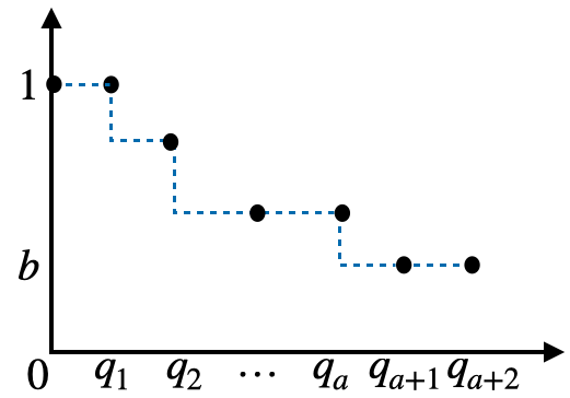
(c) 3 steps

Figure 3: Examples of Distributions with Different Number of Steps

We then prove the optimal $\mathbf{q}^{*}$ must have exactly one step by showing that for any distribution with more than $1$ steps, we can always remove one step to obtain a distribution with a lower objective function. So the optimal distribution has at most one step. Figure 4 illustrates the step removal approach. For any $k$ such that $q_{k-1}>q_{k}>q_{k+1}$, we show increasing $q_{k}$ to $q_{k-1}$ or decreasing $q_{k}$ to $q_{k+1}$ yields a lower objective function. In either case, we remove one step.

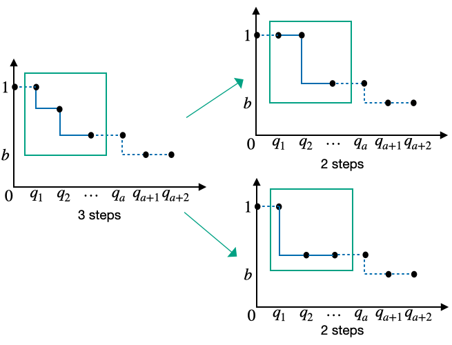
Figure 4: Step Removal

Remark 4.9

Note that Lemma 4.7 assumes that $p(\mu_{T}-a)\leq x_{i}$. If, instead, $p(\mu_{T}-a)>x_{i}$, we then consider a new distribution $D_{T}^{\prime}$ with a mean $\mu_{T}^{\prime}$ such that $p(\mu_{T}^{\prime}-a)=x_{i}$. $D_{T}^{\prime}$ is constructed as follows:$P_{D_{T}^{\prime}}(T=k)=\beta P_{D_{T}}(T=k)$ for $k\in\mathbb{Z}^{+}$, where $\beta=\frac{x_{i}}{p(\mu_{T}-a)}$. From our derivation,

$$\mathbb{E}_{T\sim D_{T}}[Z_{i}(p,T-a)\mathbbm{1}\{T\geq a\}]\geq\mathbb{E}_{T\sim D_{T}^{\prime}}[Z_{i}(p,T-a)\mathbbm{1}\{T\geq a\}]\geq\frac{1}{e}p(\mu_{T}^{\prime}-a)=\frac{1}{e}\min\{x_{i},p(\mu_{T}-a)\}$$

Here the first inequality holds since $D_{T}^{\prime}$ has more probability mass only on $0$ compared to $D_{T}$. The second inequality follows from Lemma 4.7.

4.3 Processing ‘bad’ Products

Let $\mathbf{c}^{1}$ denote the inventory obtained in Section 3, then we have shown that if $\mathbf{x}^{\mathbf{c}^{1}}\in\mathbb{Z}^{+}$, then $f(\mathbf{x}^{\mathbf{c}^{1}},T)\geq(1-\frac{1}{e})f^{\text{LP}}(\mathbf{c},T)$ and $\mathbb{E}_{T}[f(\mathbf{x}^{\mathbf{c}^{1}},T)]\geq\frac{1}{e}f^{\text{LP}}(\mathbf{c},\mu_{T})$. However, in general, $\mathbf{x}^{\mathbf{c}^{1}}$ may not be an integer-valued vector. Since $f^{\text{LP}}(\mathbf{c}^{1},T)=\textsc{fp}(\mathbf{x}^{\mathbf{c}^{1}},T)$ and the constant factor gap between fp and $f$, we essentially want to find an integer-valued vector $\mathbf{x}\in\mathcal{F}$ such that changing the starting inventory from $\mathbf{x}^{\mathbf{c}}$ to $\mathbf{x}$ does not significantly decrease fp. Recall that according to the generalized revenue-ordered structure of $\mathbf{x}^{\mathbf{c}^{1}}$ (Lemma 2.2), at most one product, specifically the one with the lowest price in $\mathbf{x}^{\mathbf{c}}$, may have fractional inventory. We refer to this item as the ‘bad’ item. Using the Separability Lemma, we show that a simple rounding of the inventory of this ‘bad’ item results in a revenue loss in fp bounded by a factor of at most $\frac{1}{T+1}$ for any $T$. The rounding procedure is formalized in the following algorithm.

1 Input: Inventory $\mathbf{c}\in\mathbb{Z}^{n}$, products sorted by the descending order of price $\mathbf{N}$:$r_{1}\geq r_{2}\geq\dots\geq r_{n}$, number of customers $T$;

2 Output: $\arg\max_{\mathbf{x}\in\{\bar{\mathbf{x}},\underline{\mathbf{x}}\}}\textsc{fp}(\mathbf{x},T)$;

3 Calculate the generalized revenue-ordered inventory $\mathbf{x}^{\mathbf{c}}$ ;

4 Let $i$ denote the index of the product with fractional inventory;

Construct $\bar{\mathbf{x}}$ and $\underline{\mathbf{x}}$ as follows:for all indices $k<i$, $\bar{x}_{k}=\underline{x}_{k}=x_{k}$; $\bar{x}_{i}=\lceil x_{i}\rceil$, $\underline{x}_{i}=\lfloor x_{i}\rfloor$; for all indices $k>i$, $\bar{x}_{k}=\underline{x}_{k}=0$.

Algorithm 4 Transformation for da with deterministic $T$

In this algorithm, we keep the inventory of other products except the ‘bad’ item unchanged, and round the inventory of the ‘bad’ item up or down based on which one has a higher revenue in the fluid process. This algorithm is computationally efficient. Calculating $\mathbf{x}^{\mathbf{c}}$ can be done in $O(n\log n)$ time by using our fast algorithm to solve CDLP (see Appendix LABEL:app:fast_cdlp) and calculating $\textsc{fp}(\mathbf{x}^{\mathbf{c}},T)$ takes $O(n)$ time using a straightforward sequencing algorithm (details in Appendix 7.2 for details.

Lemma 4.10

Given any $\mathbf{c}\in\mathbb{Z}_{+}^{n}$ and $T$, let $\mathbf{c}^{\text{ALG}}\in\mathbb{Z}_{+}^{n}$ denote the output of Algorithm 4, then $\textsc{fp}(\mathbf{c}^{\text{ALG}},T)\geq(1-\frac{1}{T+1})\textsc{fp}(\mathbf{x}^{\mathbf{c}},T)$.

To prove this lemma, it suffices to show $\max\{\textsc{fp}(\bar{\mathbf{x}},T),\textsc{fp}(\underline{\mathbf{x}},T)\}\geq(1-\frac{1}{T+1})\textsc{fp}(\mathbf{x}^{\mathbf{c}},T)$. We use the Separability Lemma to evaluate how keeping or discarding the fractional part of item $i$ affects total revenue in fp and formulate a factor-revealing mathematical program to analyze the ratio of $\max\{\textsc{fp}(\bar{\mathbf{x}},T),\textsc{fp}(\underline{\mathbf{x}},T)\}$ to $\textsc{fp}(\mathbf{x}^{\mathbf{c}},T)$. We show the optimal objective value of the factor-revealing program is $1-\frac{1}{T+1}$. An important observation used in analyzing the factor-revealing program is that the ‘bad’ item $i$ has the lowest price. The detailed proof can be found in Appendix LABEL:app:4-prf-T1.

Combining Lemma 4.5 and Lemma 4.10, we have $f(\mathbf{c}^{ALG},T)\geq(1-\frac{1}{e})(1-\frac{1}{T+1})f^{\text{LP}}(\mathbf{c},T)$. For stochastic $T$, replacing $T$ in Algorithm 4 with $\mu_{T}$ yields a $f(\mathbf{c}^{ALG},\mu_{T})\geq(1-\frac{1}{\mu_{T}+1})f^{\text{LP}}(\mathbf{c},\mu_{T})$. Combining with Lemma 4.6, we have the overall performance guarantee of $(1-\frac{1}{\mu_{T}+1})\frac{1}{e}$. Note the factors depend on $T$ ($\mu_{T}$) and increase as $T$ ($\mu_{T}$) increase. For small $T$ ($\mu_{T}$) values, we do not use the output of the algorithms described in this section. Instead, we simply stock one unit of each product in the optimal static assortment. We will discuss the details later in Section 5.1.

5 Approximation Guarantees and Runtime Analysis

In this section, we analyze the overall performance guarantee and runtime of our algorithmic framework. Then we discuss how to accelerate the algorithms further.

5.1 Overall Performance Guarantees

Theorem 5.1

Consider any accuracy level $\epsilon\in(0,1)$. When $T$ is deterministic, da can be approximated within a factor of $0.32-\epsilon$ under a cardinality or budget constraint. When $T$ is stochastic and follows a distribution with the IFR property, da can be approximated within a factor of $0.194-\epsilon$ under a cardinality or budget constraint.

We show how to establish the guarantee under a cardinality constraint while the proofs for the budget constraint are similar and deferred to Appendix LABEL:app:5.

When $T$ is deterministic, combining Theorem 3.1 and the results in Section 4.3, we obtain an inventory vector $\mathbf{c}^{ALG}$ such that $f(\mathbf{c}^{ALG},T)\geq\left((1-\frac{1}{e})^{2}(1-\frac{1}{T+1})-\epsilon\right)\max_{\|\mathbf{c}\|\leq K}f^{\text{LP}}(\mathbf{c},T)$. Since $f^{\text{LP}}(\mathbf{c},T)$ is an upper bound for $f(\mathbf{c},T)$ (See Section 2), $\mathbf{c}^{ALG}$ provides a $\frac{1}{2}(1-\frac{1}{e})(1-\frac{1}{T+1})-\epsilon$-approximate solution. Note this approximation factor increases as $T$ decreases. For small values of $T$, we stock the static assortment as the starting inventory, $\mathbf{c}^{\text{static}}=\arg\max_{\|\mathbf{c}\|\leq K}f^{\text{LP}}(\mathbf{c},1)$. Given that the expected revenue obtained from each customer starting from the optimal inventory is less than the expected revenue of the static assortment, we have $\max_{\|\mathbf{c}\|\leq K}f(\mathbf{c},T)\leq Tf(\mathbf{c}^{\text{static}},1)$. Due to the monotonicity of $f(\mathbf{c},t)$ in $t$, it follows that $f(\mathbf{c}^{\text{static}},T)\geq f(\mathbf{c}^{\text{static}},1)\geq\frac{1}{T}\max_{\|\mathbf{c}\|\leq K}f(\mathbf{c},T)$. When $T<4$, we use $\mathbf{c}^{\text{static}}$ as the starting inventory while we use $\mathbf{c}^{ALG}$ when $T\geq 4$. Thus, the worst-case performance guarantee is $\max\{\frac{1}{3}-\epsilon,(1-\frac{1}{e})^{2}\frac{4}{5}-\epsilon\}=0.32-\epsilon$.

When $T$ is stochastic, combining Theorem 3.1 and the results in Section 4.3, we obtain an inventory vector $\mathbf{c}^{ALG}$ such that $\mathbb{E}_{T}[f(\mathbf{c}^{ALG},T)]\geq\frac{1}{e}(1-\frac{1}{\mu_{T}+1})\max_{\|\mathbf{c}\|\leq K}f^{\text{LP}}(\mathbf{c},\mu_{T})$. Therefore, we have $\mathbb{E}_{T}[f(\mathbf{c}^{ALG},T)]\geq((1-\frac{1}{e})\frac{1}{e}(1-\frac{1}{\mu_{T}+1})-\epsilon)\max_{\|\mathbf{c}\|\leq K}f^{\text{LP}}(\mathbf{c},\mu_{T})\geq((1-\frac{1}{e})\frac{1}{e}(1-\frac{1}{\mu_{T}+1})-\epsilon)\max_{\|\mathbf{c}\|\leq K}\mathbb{E}_{T}[f(\mathbf{c},T)]$. Here the last inequality is from Proposition 7.4 that $f^{\text{LP}}(\mathbf{c},\mu_{T})$ is an upper bound for $f(\mathbf{c},T)$. Similar to deterministic $T$, when $\mu_{T}<5.15$, we use $\mathbf{c}^{\text{static}}$ as the starting inventory while we use $\mathbf{c}^{\text{DA}}$ when $\mu\geq 5.15$. Thus, the worst-case performance guarantee is $\frac{1}{5.15}-\epsilon=0.194-\epsilon$.

Next, we summarize the performance guarantee of dap problem as follows, which is a straightforward combination of Section 3.3 and Section 4.1.

Theorem 5.2

Given any accuracy level $\epsilon\in(0,1)$, when $T$ is deterministic, dap can be approximated within a factor of $\frac{1}{2}(1-\frac{1}{e})-\epsilon$ under a cardinality constraint and $\frac{1}{3}(1-\frac{1}{e})-\epsilon$ under a budget constraint. When $T$ is stochastic, for any distribution of $T$, dap can be approximated within a factor of $\frac{1}{4}-\epsilon$ under a cardinality constraint and $\frac{1}{6}-\epsilon$ under a budget constraint.

5.2 Runtime Analysis and Acceleration

Recall that our algorithm framework has two steps. In the second step for both da and dap, we need only to solve the CDLP or a static assortment optimization problem, both of which can be done in polynomial time. Therefore, our primary focus will be on the first step and we will focus on the cardinality constraint.

Recall for da, we try $\lceil\log_{1+\epsilon}\frac{K}{\epsilon}\rceil$ values of $y_{0}$. For each value of $y_{0}$, we use the standard greedy algorithm to maximize the monotone and submodular functions. In each iteration, we calculate the marginal benefit for all products and add one unit of the product with the maximum marginal benefit. Since $y_{0}$ is given, calculating the marginal benefit of each product is equivalent to solving a fractional knapsack problem. Since only the inventory of one product changes,it takes $O(\log n+n)$ time to update the sorting and solve the knapsack problem. Thus, the overall time complexity is $O(n^{2}K\log_{1+\epsilon}\frac{K}{\epsilon})$.

For dap, recall that in the first step, we iterate over all items in the expanded set and calculate the maximum marginal benefit of each item. The number of queries to calculate the marginal benefit can be very large when the expanded ground set is large. We accelerate the algorithm by iterating only over different products in the ground set (instead of the expanded ground set with many copies) and deciding the inventory of each product. The the query complexity reduces to $O(\epsilon^{-1}n\log n)$. Moreover, when examining each product, we use binary search to determine the quantity to add to the inventory. The binary search relies on the fact that the marginal benefit is non-increasing when adding more units of each product. The time complexity of the binary search is $O(mn\log(mn))$ for deterministic $T$. The algorithm details and runtime analysis are deferred to Appendix LABEL:app:acc. Thus, the total runtime is $O(\epsilon^{-1}n\log n(mn\log mn+\log K))$. For stochastic $T$, the only difference is just that we need to evaluate the expectation of the marginal benefit over $T$ when examining each product. This results in the same overall run time of $O(\epsilon^{-1}T_{max}n\log n(mn\log mn+\log K))$.

6 Conclusion

In this work, we consider a dynamic assortment optimization problem under the MNL choice model. We develop a unified approximation algorithmic framework for both da and dap. This framework outperforms existing approximation algorithms in terms of speed, approximate guarantees, and also accommodates multiple constraints and a stochastic number of customers. From a technical perspective, we believe that our algorithmic ideas and the novel structural properties of the MNL model can shed light on algorithm design for assortment planning and broader revenue management problems. Further research can consider extending this approximation to other choice models, such as the Nested Logit and Markov Chain choice models. Additionally, we point out that approximating da for general distributions (in polynomial time) remains an interesting open problem.

Endnotes

1. 1 Assuming the existence of an efficient oracle, the algorithm in Aouad et al. (2018) provides a $(0.139-\epsilon)-$approximate solution with a probability of at least $1-\delta$ for any $\epsilon\in(0,1/4)$ and $\delta>0$. Here $\epsilon$ is a parameter of the accuracy level we can set. To the best of our knowledge, the existence of the oracle remains an open problem. Moreover, our algorithm offers a better approximation guarantee than this result.

7 Additional Formulations and Proofs in Section 2

7.1 Proof of lemma 2.1

The proof is based on Lemmas 8 and 10 of Goyal et al. (2022), as detailed below.

Lemma 7.1 (Lemma 8 and 10 in Goyal et al. (2022))

Given any feasible solution $\{y_{i}\}_{i\in\mathbf{N}\cup\{0\}}$ to the sales-based formulation of CDLP (2) with inventory $\mathbf{c}$ and periods $T$, let $x_{i}=y_{i}$ for all $i\in\mathbf{N}$. Then $\textsc{fp}(\mathbf{x},T)=\sum_{i\in\mathbf{N}}r_{i}y_{i}$.

This lemma essentially says that if we set the starting inventory of each product as a feasible solution to the sales-based CDLP, then the inventory will be depleted within the selling horizon. Therefore, the revenue in fp is equal to the objective function of the CDLP.

Proof 7.2

Proof of Lemma 2.1. We show that given any feasible solution to $f^{\text{LP}}$, one can construct a feasible solution to $\max_{\mathbf{x}\preceq\mathbf{c}}\textsc{fp}(\mathbf{x},T)$ with the same objective function value and vise versa.

Let $\{y_{i}\}_{i\in\mathbf{N}\cup\{0\}}$ denote a feasible solution to CDLP. Then if we set $\mathbf{x}$ by $x_{i}=y_{i}$, $\mathbf{x}$ is a feasible solution to $\max_{\mathbf{x}\preceq\mathbf{c}}\textsc{fp}(x,T)$ since $x_{i}=y_{i}\leq c_{i}$. Moreover, from Lemma 7.1, all inventory in $\mathbf{x}$ will be depleted, thus $\textsc{fp}(x,T)=\sum_{i\in\mathbf{N}}{r_{i}y_{i}}$.

Let $\mathbf{x}$ be a feasible solution to $\max_{\mathbf{x}\preceq\mathbf{c}}FP(x,T)$, so $x_{i}\leq c_{i}$ for all $i\in\mathbf{N}$. Then let $y_{i}=Z^{\text{FP}}_{i}(\mathbf{x},T)$ for all $i\in\mathbf{N}\cup\{0\}$ ($Z^{\text{FP}}_{0}(\mathbf{x},T)$ is the number of customers who do not make purchases). Obviously, $\textsc{fp}(\mathbf{x},T)=\sum_{i\in\mathbf{N}}r_{i}Z^{\text{FP}}_{i}(\mathbf{x},T)=\sum_{i\in\mathbf{N}}r_{i}y_{i}$. So, we just need to show that $\{y_{i}\}_{i\in\mathbf{N}}$ is a feasible solution to CDLP, i.e, $y_{i}\leq y_{0}\frac{v_{i}}{v_{0}}$, $y_{i}\leq c_{i}$. Since $Z^{\text{FP}}_{i}(\mathbf{x},T)$ is the consumption of $i$ in $\textsc{fp}(\mathbf{x},T)$ and $\mathbf{x}\preceq\mathbf{c}$, we have $Z^{\text{FP}}_{i}(\mathbf{x},T)\leq x_{i}\leq c_{i}$. Due to the Independence of Irrelevant Alternatives (IIA) property, we have $Z^{\text{FP}}_{i}(\mathbf{x},T)\leq Z^{\text{FP}}_{i}(\mathbf{x},T)\frac{v_{i}}{v_{0}}$. So $y_{i}\leq y_{0}\frac{v_{i}}{v_{0}}$, $y_{i}\leq c_{i}$ for all $i\in\mathbf{N}$.

7.2 Sequencing Algorithm

The Sequencing algorithm is introduced in Goyal et al. (2022), the algorithm outputs a nested sequence of assortments that appear in the fluid process and their time durations.

Input: products sorted in descending order of price $\mathbf{N}$, number of customers $T$, inventory $\mathbf{c}$

Output: sequence of assortments $\{S_{l}\}_{l=1}^{L}:S_{L}\subseteq\dots\subseteq S_{2}\subseteq S_{1}$, durations of each assortment$\{t_{l}\}_{l=1}^{L}$

1 Initialize $t=0$, $l=1$;

2 while $S_{l}\neq\emptyset$ and $t\leq T$ do

3      $S_{l}=\{i\in\mathbf{N}|c_{i}>0\}$, $t_{l}=\text{min}\{\min_{i\in\mathbf{N}}\frac{x_{i}}{\phi(i,S_{l})}$, $T-t$} ;

4      for  $i\in\mathbf{N}$  do  $c_{i}=c_{i}-t_{l}\phi(i,S)$ ;

5      $l=l+1$, $t=t+t_{l}$

6      if $t<T$ then  $S_{l}=\emptyset,t_{l}=T-t$ ;

Algorithm 5 Sequencing

In the algorithm, $S_{l}$ is the $l$th assortment appearing in the fluid process. In Line 3, $\min_{i\in\mathbf{N}}\frac{x_{i}}{\phi(i,S_{l})}$ calculates the first product that stocks out after current time $t$.

7.3 Proof of Lemma 2.2

Proof 7.3

Proof of Lemma 2.2. When $y_{0}^{*}$ is fixed, the problem simplifies to a knapsack problem:

$$\max_{\mathbf{y}\in\mathbb{R}^{n+1}_{+}}\left\{\sum_{i\in\mathbf{N}}r_{i}y_{i}:\sum_{i\in\mathbf{N}}y_{i}+y_{0}^{*}=T,y_{i}\leq c_{i},y_{i}\leq y_{0}\frac{v_{i}}{v_{0}},\forall i\in\mathbf{N}\right\}$$

This is a knapsack problem, so there exists an optimal solution satisfying the following structure:There is an item $i_{\tau}$, such that $y_{i}^{*}=\min\{c_{i},y_{0}^{*}\frac{v_{i}}{v_{0}}\}$ for $i<i_{\tau}$, $y_{i}^{*}=0$ for $i>i_{\tau}$, and $y_{i_{\tau}}^{*}=T-y_{0}^{*}-\sum_{i=1}^{i_{\tau}-1}y_{i}<\min\{c_{i},y_{0}^{*}v_{i_{\tau}}\}$. Given the starting inventory $\mathbf{x}$, where $x_{i}=y_{i}^{*}$ for all $i\in N(\mathbf{c})\cup\{0\}$, according to Lemma 7.1, all the inventory in $\mathbf{x}$ will be depleted, $Z^{\text{FP}}_{i}(\mathbf{x},T)=y_{i}^{*}$. Consequently, $\textsc{fp}(\mathbf{x},T)=\sum_{i\in\mathbf{N}}r_{i}Z^{\text{FP}}_{i}(\mathbf{x},T)=\sum_{i\in\mathbf{N}}r_{i}y_{i}^{*}=f^{\text{LP}}(\mathbf{c},T)$. Therefore, to prove this lemma, it suffices to show that $\textsc{fp}(\mathbf{x},T)=\textsc{fp}(\mathbf{x}^{\mathbf{c}},T)$.

Note the difference between $\mathbf{x}$ and $\mathbf{x}^{\mathbf{c}}$ arises only for $i<i_{\tau}$, where $x_{i}(\mathbf{c})=c_{i}\geq\min\{c_{i},y_{0}^{*}\frac{v_{i}}{v_{0}}\}=x_{i}$. If $c_{i}<y_{0}^{*}\frac{v_{i}}{v_{0}}$, then $x_{i}=c_{i}=x_{i}(\mathbf{c})$. For $c_{i}>y_{0}^{*}\frac{v_{i}}{v_{0}}$, product $i$ is available until the end of the fluid process $\textsc{fp}(\mathbf{c},T)$. Thus, adding more units of item $i$ does not alter the fluid process. Hence, $\textsc{fp}(\mathbf{x}^{\mathbf{c}},T)=\textsc{fp}(\mathbf{x},T)=f^{\text{LP}}(\mathbf{c},T)$.

7.4 Proposition 7.4

Proposition 7.4

$f^{\text{LP}}(\mathbf{c},\mu_{T})$ serves as an upper bound to $\mathbb{E}_{T}[f(\mathbf{c},T)]$.

Proof 7.5

Proof of Proposition 7.4. The proof is an adaptation from Liu and Van Ryzin (2008) and the key is to show we can construct a feasible solution to $f^{\text{LP}}(\mathbf{c},\mu_{T})$ that provides an upper bound for $\mathbb{E}_{T}[f(\mathbf{c},T)]$.

Consider a setting where the assortment can be dynamically adjusted, with the assortment policy denoted as $\pi$. This policy is a function of time $t$, the total number of customers $T$, and the purchase history $\mathcal{H}$. Let $V^{*}$ represent the optimal expected revenue in this scenario. Since dynamic assortment adjustment is allowed in this setting but not allowed in da, $V^{*}\geq\mathbb{E}_{T}[f(\mathbf{c},T)]$.

Let $S_{\pi}(t,T)$ denote the assortment offered under policy $\pi$ at time $t$ when there are $T$ customers, with implicit dependence on the purchase history. Define $X_{i}(S_{\pi}(t,T))$ as an indicator function, where $X_{i}(S_{\pi}(t,T))=1$ if product $i$ is purchased by the $t$th customer when assortment $S_{\pi}(t,T)$ is offered and $0$ otherwise. Then $V^{*}$ can be expressed as follows:

$$V^{*}= \max_{\pi}\mathbb{E}_{T}\mathbb{E}[\sum_{t=1}^{T}\sum_{i\in\mathbf{N}}r_{i}X_{i}(S_{\pi}(t,T))]$$

$$\text{s.t.}\sum_{t=1}^{T}X_{i}(S_{\pi}(t,T))\leq c_{i}\quad\forall T,i\in\mathbf{N}\quad(\text{pathwise})$$

$$S_{\mu_{T}}(t,T)\subseteq N,\quad\forall T\quad\forall t=1,\dots,T$$

Here the expectation in the objective function is taken over $T$ and all possible sample paths. The first constraint is path-wise, ensuring that the total consumption of each product does not exceed its inventory on any sample path. Taking the expectation over the sample paths and $T$, we get $\mathbb{E}_{T}\mathbb{E}[\sum_{t=1}^{T}X_{i}(S_{\pi}(t,T))]\leq c_{i}$ for all $i$.

Let $\pi^{*}$ denote the optimal policy of the following optimization problem. Let $y_{\pi^{*}}(S)=\mathbb{E}_{T}\mathbb{E}[\sum_{t=1}^{T}\mathbbm{1}\{S_{\pi^{*}}(t,T)=S\}]$. Then, $\sum_{S\subseteq N}\phi(i,S)y_{\pi^{*}}(S)=\mathbb{E}_{T}\mathbb{E}[\sum_{t=1}^{T}X_{i}(S_{\pi}(t,T))]\leq c_{i}$. Moreover, $\sum_{S\subseteq N}y_{\pi^{*}}(S)\leq\mu_{T}$ as $\sum_{S\subseteq N}\mathbb{E}[\sum_{t=1}^{T}\mathbbm{1}\{(S_{\pi^{*}}(t,T))=S\}]\leq T$ for each $T$. Therefore, $\{y_{\pi^{*}}(S)\}_{S\subseteq\mathbf{N}}$ is a feasible solution to $f^{\text{LP}}(\mathbf{c},\mu_{T})$. Furthermore, $V^{*}=\mathbb{E}_{T}\mathbb{E}[\sum_{t=1}^{T}\sum_{i\in\mathbf{N}}r_{i}X_{i}(S_{\pi^{*}}(t,T))]=\sum_{S\subseteq\mathbf{N}}\sum_{i\in\mathbf{N}}y_{\pi^{*}}(S)\phi(i,S)r_{i}$. So $f^{\text{LP}}(\mathbf{c},\mu_{T})\geq V^{*}$. Since $V^{*}\geq\mathbb{E}_{T}[f(\mathbf{c},T)]$, we have $f^{\text{LP}}(\mathbf{c},\mu_{T})\geq\mathbb{E}_{T}[f(\mathbf{c},T)]$.

7.5 Multi-type CDLP Formulation

We first provide the choice-based formulation. Let $\{y_{k}(S)\}_{k\in\mathbf{M},S\subseteq\mathbf{N}}$ represent the probability of offering assortment $S$ to a customer of type $k$.

$$\begin{split}f^{\text{LP}}_{\mathbf{M}}(\mathbf{c},T)&=\max_{\mathbf{y}}T\lambda_{k}\sum_{S\subseteq\mathbf{N}}\sum_{k\in\mathbf{M}}y_{k}(S)R_{k}(S)\\ \text{s.t. }&T\lambda_{k}\sum_{k\in\mathbf{M}}\sum_{S\subseteq\mathbf{N}}y_{k}(S)\lambda_{k}\phi_{k}(i,S)\leq c_{i},\forall i\in\bf{N}\\ &\sum_{S\subseteq\bf{N}}y_{k}(S)=1,\forall k\in\mathbf{M}\\ &y(S)\geq 0,\forall S\subseteq\bf{N}\end{split}$$ (11)

Here $\lambda_{k}=\mathbb{E}[\lambda_{k,t}]$, and $T\lambda_{k}$ is the expected number of type $k$ customers. The objective function maximizes the total expected revenue from $T$ customers. The first constraint ensures that the inventory of product $i$ does not exceed $c_{i}$. The second constraint ensures that the sum of the probability of the assortments offered to each customer is $1$ (including the empty set).

Below is the equivalent sales-based formulation of multi-type CDLP. Let $y_{ki}$ denote the sales of product $i$ for type $k$ customers.

$$\begin{split}f^{\text{LP}}_{\mathbf{M}}(\mathbf{c},T)&=\max_{\mathbf{y}\geq\mathbf{0}}\sum_{k\in\mathbf{M},i\in\mathbf{N}}r_{i}y_{ki}\\ \text{s.t. }&\sum_{k\in\mathbf{M}}y_{ki}\leq c_{i}\quad\forall i\in\mathbf{N}\\ &\sum_{i\in\mathbf{N}}y_{ki}+y_{k0}\leq T\lambda_{k}\quad\forall k\in\mathbf{M}\\ &y_{ki}\leq y_{ki}\frac{v_{ki}}{v_{k0}}\quad\forall i\in\mathbf{N},\forall k\in\mathbf{M}\end{split}$$ (12)

The objective function maximizes the total expected revenue for $T$ customers. Here the first constraint ensures that the inventory of product $i$ cannot exceed $c_{i}$. The second constraint ensures that the total sales of all products, including the pseudo product $0$, cannot exceed the number of customers. The third constraint describes the relationship between the sales of different products under the MNL choice model.

8 Algorithms, Lemmas, and Proofs in Section 3

8.1 Proof of Theorem 3.1

The following proposition shows that $g(\mathbf{c},y_{0})$ is a submodular function when $y_{0}$ is fixed.

Proposition 8.1 (Theorem 4.3 in Bai et al. (2022))

For each $i\in\mathbf{N}$, given a feasible $\bar{y}_{0}$, and $\mathbf{c},\mathbf{b}\in\mathbb{Z}_{+}^{n}$ where $\mathbf{c}\geq\mathbf{b}$, it holds that $g(\mathbf{c}+\mathbf{e}_{i},\bar{y}_{0})-g(\mathbf{c},\bar{y}_{0})\leq g(\mathbf{b}+\mathbf{e}_{i},\bar{y}_{0})-g(\mathbf{b},\bar{y}_{0})$.

We first present the algorithm and then prove Theorem 3.1.

1 Input: Cardinality $K$, error $\epsilon\in(0,1)$, products sorted by descending order of price $\mathbf{N}$:$r_{1}\geq r_{2}\geq\dots\geq r_{n}$, number of customers $T$;

2 Output:$\mathbf{c}^{ALG}$;

3 for $u\leftarrow 1$ to $\lceil log_{1+\epsilon}\frac{T}{\epsilon}\rceil$ do

4      $\mathbf{c}^{u}=\text{Cardinality-constrained Submodular Max}(K,(1+\epsilon)^{k-1}\epsilon,g,\mathbf{N})$;

5     

return $\mathbf{c}=\text{Best of }\mathbf{c}^{1}$, $\mathbf{c}^{2}$, …, $\mathbf{c}^{\lceil log_{1+\epsilon}\frac{T}{\epsilon}\rceil}$

Algorithm 6 Cardinality Opt for da

1 Input: Budget $B$, weight $(b_{i})_{i\in\mathbf{N}}$, products sorted by descending order of price $\mathbf{N}$:$r_{1}\geq r_{2}\geq\dots\geq r_{n}$, error $\epsilon\in(0,1)$, number of customers $T$;

2 Output:$\mathbf{c}^{ALG}$;

3 for $i\leftarrow 1$ to $\lceil log_{1+\epsilon}\frac{T}{\epsilon}\rceil$ do

4      $\mathbf{c}^{i}=\text{Budget-constrained Submodular Max}(K,(1+\epsilon)^{i-1}\epsilon,g,\mathbf{N})$;

5     

return $\mathbf{c}=\text{Best of }\mathbf{c}^{1}$, $\mathbf{c}^{2}$, …, $\mathbf{c}^{\lceil log_{1+\epsilon}\frac{T}{\epsilon}\rceil}$

Algorithm 7 Budget Opt for da Fluid Relaxation

In these algorithms, we try $\lceil log_{1+\epsilon}\frac{T}{\epsilon}\rceil$ values of $y_{0}$, ranging from $\epsilon$ to $T$. For each specified $y_{0}$, we apply a standard algorithm for maximizing a monotone submodular function $g$ under either a cardinality constraint or budget constraint to find an approximate inventory $\mathbf{c}^{i}$. Finally, we return the inventory vector with the highest $g$ value. Next, we establish the approximation guarantee.

Proof 8.2

Proof of Theorem 3.1. Let $y_{0}^{u}=\epsilon(1+\epsilon)^{u-1}$. For any $y_{0}$, we use $\mathbf{c}^{ALG}(y_{0})$ to denote the output inventory vector of the submodular maximization algorithm given $y_{0}$ and let $\mathbf{c}^{\text{OPT}}(y_{0})$ denote the optimal inventory for $g$ given $y_{0}$, i.e., $\mathbf{c}^{\text{OPT}}(y_{0})=\arg\max_{\mathbf{c}\in\mathcal{F}}g(\mathbf{c},y_{0})$. Let $\mathbf{c}^{\text{OPT}}$ denote the optimal inventory for the original problem:$\max_{\mathbf{c}\in\mathcal{F}}f^{\text{LP}}(\mathbf{c},T)$. Let $y_{0}^{\text{OPT}}$ denote the value of $y_{0}$ in the optimal solution of $f^{\text{LP}}(\mathbf{c}^{\text{OPT}},T)$. Since $y_{0}\in(0,T)$, there exists an $i$ such that $y_{0}^{\text{OPT}}(1-\epsilon)\leq y_{0}^{u}\leq y_{0}^{\text{OPT}}$, implying there exists $0\leq\epsilon^{\prime}<\epsilon$, such that $y_{0}^{u}=(1-\epsilon^{\prime})y_{0}^{\text{OPT}}$. Then we have:

$$g(\mathbf{c}^{ALG}(y_{0}^{u}),y_{0}^{u}) \geq(1-\frac{1}{e})g(\mathbf{c}^{\text{OPT}}(y_{0}^{u}),y_{0}^{u})$$

$$\geq(1-\frac{1}{e})g(\mathbf{c}^{\text{OPT}}(y_{0}^{\text{OPT}}),y_{0}^{u})$$

$$=(1-\frac{1}{e})g(\mathbf{c}^{\text{OPT}}(y_{0}^{\text{OPT}}),(1-\epsilon^{\prime})y_{0}^{\text{OPT}})$$ (13)

Here the first inequality is from the standard submodular maximization algorithm. The second inequality holds since $\mathbf{c}^{\text{OPT}}(y_{0}^{u})$ is the optimal inventory for $g$ given $y_{0}^{u}$. The equation is derived by plugging in $y_{0}^{u}=(1-\epsilon^{\prime})y_{0}^{\text{OPT}}$.

Observe that $g(\mathbf{c},y_{0})$ is a knapsack problem that the weight of each product is $\min\{y_{0}\frac{v_{i}}{v_{0}},c_{i}\}$. Let $\{y_{i}\}_{i\in\mathbf{N}}$ denote the optimal solution of the knapsack problem $g(\mathbf{c}^{\text{OPT}}(y_{0}^{\text{OPT}}),y_{0}^{\text{OPT}})$. From the structure of the optimal solution to a knapsack problem, the optimal solution will include the high-price products until the total weights is $T$. So we have

$$g(\mathbf{c}^{\text{OPT}}(y_{0}^{\text{OPT}}),y_{0}^{\text{OPT}})=\sum_{i\in\mathbf{N}:y_{i}=\min\{\frac{v_{i}}{v_{0}}y_{0}^{\text{OPT}},c_{i}\}}r_{i}\min\{\frac{v_{i}}{v_{0}}y_{0}^{\text{OPT}},c_{i}\}+\sum_{i\in\mathbf{N}:0<y_{i}<\min\{\frac{v_{i}}{v_{0}}y_{0}^{\text{OPT}},c_{i}\}}r_{i}y_{i}$$ (14)

When $y_{0}^{\text{OPT}}$ decreases to $y_{0}^{\text{OPT}}(1-\epsilon^{\prime})$, the weights of the products in the knapsack problem will change, thus the new optimal solution $\{y_{i}^{\prime}\}_{i\in\mathbf{N}\cup\{0\}}$ will change accordingly. Moreover, only the optimal value for product $i$ that satisfies $y_{i}=\min\{\frac{v_{i}}{v_{0}}y_{0}^{\text{OPT}},c_{i}\}$ and $\frac{v_{i}}{v_{0}}y_{0}^{\text{OPT}}\geq c_{i}$ may decrease, which will become $y_{i}^{\prime}=\min\{\frac{v_{i}}{v_{0}}y_{0}^{\text{OPT}}(1-\epsilon^{\prime}),c_{i}\}$. So we have the following:

$$g(\mathbf{c}^{\text{OPT}}(y_{0}^{\text{OPT}}),(1-\epsilon^{\prime})y_{0}^{\text{OPT}})$$

$$\geq g(\mathbf{c}^{\text{OPT}}(y_{0}^{\text{OPT}}),y_{0}^{\text{OPT}})-\sum_{i\in\mathbf{N}:y_{i}=\min\{\frac{v_{i}}{v_{0}}y_{0}^{\text{OPT}},c_{i}\}}r_{i}(\min\{\frac{v_{i}}{v_{0}}y_{0}^{\text{OPT}},c_{i}\}-\min\{\frac{v_{i}}{v_{0}}y_{0}^{\text{OPT}}(1-\epsilon^{\prime}),c_{i}\})$$

$$\geq g(\mathbf{c}^{\text{OPT}}(y_{0}^{\text{OPT}}),y_{0}^{\text{OPT}})-\epsilon^{\prime}\sum_{i\in\mathbf{N}:y_{i}=\min\{\frac{v_{i}}{v_{0}}y_{0}^{\text{OPT}},c_{i}\}}r_{i}\min\{\frac{v_{i}}{v_{0}}y_{0}^{\text{OPT}},c_{i}\}$$

$$\geq(1-\epsilon^{\prime})g(\mathbf{c}^{\text{OPT}}(y_{0}^{\text{OPT}}),y_{0}^{\text{OPT}})$$

$$=(1-\epsilon^{\prime})f^{\text{LP}}(\mathbf{c}^{\text{OPT}},T)$$

The second inequality holds since for any product $i$, $\min\{\frac{v_{i}}{v_{0}}y_{0}^{\text{OPT}},c_{i}\}-\min\{\frac{v_{i}}{v_{0}}y_{0}^{\text{OPT}}(1-\epsilon^{\prime}),c_{i}\}\leq\min\{\frac{v_{i}}{v_{0}}y_{0}^{\text{OPT}},c_{i}\}-(1-\epsilon^{\prime})\min\{\frac{v_{i}}{v_{0}}y_{0}^{\text{OPT}},c_{i}\}=\epsilon\min\{\frac{v_{i}}{v_{0}}y_{0}^{\text{OPT}},c_{i}\}$. The last equation holds since $g(\mathbf{c}^{\text{OPT}}(y_{0}^{\text{OPT}}),y_{0}^{\text{OPT}})=f^{\text{LP}}(\mathbf{c}^{\text{OPT}},T)$. The third inequality is derived from equation (14). Combining this inequality with inequality (13), we have $f^{\text{LP}}(\mathbf{c}^{ALG}(y_{0}^{u}),T)\geq(1-\frac{1}{e}-\epsilon^{\prime})\hat{f}(\mathbf{C}^{\text{OPT}})$. Since the algorithm outputs the best approximate inventory vector, $g(\mathbf{c}^{ALG}(y_{0}^{ALG}),y_{0}^{ALG}))\geq g(\mathbf{c}^{ALG}(y_{0}^{u}),y_{0}^{u}))\geq(1-\frac{1}{e}-\epsilon)f^{\text{LP}}(\mathbf{c}^{\text{OPT}},T)$. Since the optimal solution $\{y_{i}^{*}\}_{i\in\mathbf{N}}$ and $y_{0}^{ALG}$ to $g(\mathbf{c}^{ALG}(y_{0}^{ALG}),y_{0}^{ALG}))$ is a feasible solution to $f^{\text{LP}}(\mathbf{c}^{ALG}(y_{0}^{ALG}),T)$, we have $f^{\text{LP}}(\mathbf{c}^{ALG}(y_{0}^{ALG}),T)\geq g(\mathbf{c}^{ALG}(y_{0}^{ALG}),y_{0}^{ALG}))\geq(1-\frac{1}{e}-\epsilon)f^{\text{LP}}(\mathbf{c}^{\text{OPT}},T)$.

8.2 Proof of Lemma 3.3

Proof 8.3

Proof of Lemma 3.3. First, we prove (i), and (ii) follows from (i). Consider the outside option as a pseudo product $0$, with choice probability $\phi(0,S)=\frac{v_{0}}{v_{0}+\sum_{j\in S}v_{j}}$. Then we have $\phi(S\cup\{0\})=1$ for any subset $S\subseteq\mathbf{N}$ for any subset $S\subseteq\mathbf{N}$. Therefore, the total consumption in $\textsc{fp}(\mathbf{x}+\delta_{i}\mathbf{e}_{i},T)$, including the pseudo product, always equals $T$ since $\phi(S\cup\{0\})=1$. Given that the extra consumption of product $i$, $Z^{\text{FP}}_{i}(\mathbf{x}+\delta_{i}\mathbf{e}_{i},T)-Z^{\text{FP}}_{i}(\mathbf{x},T)$, is $\alpha_{i}$, we have $\sum_{j\in\mathbf{N}\cup\{0\}\backslash\{i\}}Z^{\text{FP}}_{j}(\mathbf{x}+\delta_{i}\mathbf{e}_{i},T)+Z^{\text{FP}}_{i}(\mathbf{x},T)+\alpha_{i}=T$. Similarly, in the truncated fluid process $\textsc{fp}(\mathbf{x},T-\alpha_{i})$, we have $\sum_{j\in\mathbf{N}\cup\{0\}}Z^{\text{FP}}_{i}(\mathbf{x},T)=T-\alpha_{i}$. Thus,

$$\sum_{j\in\mathbf{N}\cup\{0\}\backslash\{i\}}Z^{\text{FP}}_{j}(\mathbf{x}+\delta_{i},T)+Z^{\text{FP}}_{i}(\mathbf{x},T)=\sum_{j\in\mathbf{N}\cup\{0\}\backslash\{i\}}Z^{\text{FP}}_{i}(\mathbf{x},T).$$

Note that the pseudo product $0$ is always available. From IIA property of MNL, the consumption of product $j$ in $\textsc{fp}(\mathbf{x}+\delta_{i}\mathbf{e}_{i},T)$ is a function of $Z^{\text{FP}}_{0}(\mathbf{x}+\delta_{i}\mathbf{e}_{i},T)$:$Z^{\text{FP}}_{j}(\mathbf{x}+\delta_{i}\mathbf{e}_{i},T)=\min(\frac{v_{j}}{v_{0}}Z_{0}(\mathbf{x}+\delta_{i}\mathbf{e}_{i},T),x_{j})$. Similarly, we have $Z^{\text{FP}}_{j}(\mathbf{x},T-\alpha_{i}\mathbf{e}_{i})=\min(\frac{v_{j}}{v_{0}}Z^{\text{FP}}_{0}(\mathbf{x},T-\alpha_{i}),x_{j})$. So we have:

$$\sum_{k\in N}\min(\frac{v_{k}}{v_{0}}Z_{0}(\mathbf{x}+\delta_{i}\mathbf{e}_{i},T),x_{k})+Z_{0}(\mathbf{x}+\delta_{i}\mathbf{e}_{i},T)=\sum_{j\in\mathbf{N}}\min(\frac{v_{k}}{v_{0}}Z^{\text{FP}}_{0}(\mathbf{x},T-\alpha_{i}),x_{k})+Z^{\text{FP}}_{0}(\mathbf{x},T-\alpha_{i}).$$

Let $h(Z_{0})=\sum_{k\in N}\min(\frac{v_{k}}{v_{0}}Z_{0},x_{k})+Z_{0}$, observe that $h(Z_{0})$ is a strictly increasing function in $Z_{0}$. Since $h(Z_{0}(\mathbf{x}+\delta_{i}\mathbf{e}_{i},T))=h(Z^{\text{FP}}_{0}(\mathbf{x},T-\alpha_{i}))$, we have $Z^{\text{FP}}_{0}(\mathbf{x}+\delta_{i}\mathbf{e}_{i},T)=Z^{\text{FP}}_{0}(\mathbf{x},T-\alpha_{i})$. Further, $Z^{\text{FP}}_{j}(\mathbf{x}+\delta_{i}\mathbf{e}_{i},T)=h(Z^{\text{FP}}_{)}(\mathbf{x}+\delta_{i}\mathbf{e}_{i},T))=h(Z^{\text{FP}}_{0}(\mathbf{x},T-\alpha_{i}))$ for all $j\in\mathbf{N}$, which means the consumption of any product except $i$ is equal between two processes.

Then we show Part (ii).

$$\textsc{fp}(\mathbf{x}+\delta_{i}\mathbf{e}_{j},T) =\sum_{j\in\mathbf{N}\cup\{i\}}r_{j}Z^{\text{FP}}_{j}(\mathbf{x}+\delta_{i}\mathbf{e}_{j},T)=\sum_{j\in\mathbf{N}}r_{j}Z^{\text{FP}}_{j}(\mathbf{x}+\delta_{i}\mathbf{e}_{j},T)+\alpha_{i}r_{i}$$

$$=\sum_{j\in\mathbf{N}}r_{j}Z^{\text{FP}}_{j}(\mathbf{x},T-\alpha_{i})+\alpha_{i}r_{i}=\textsc{fp}(\mathbf{x},T-\alpha_{i})+\alpha_{i}r_{i}.$$

Here the first equality and the last equality hold since the total revenue is the sum of revenue gained from each product. The second equality follows from the fact that we define $\alpha_{i}=Z^{\text{FP}}_{i}(\mathbf{c}+\delta_{i}\mathbf{e}_{i},T)-Z^{\text{FP}}_{i}(\mathbf{c},T)$. The third equality holds since we have shown $Z^{\text{FP}}_{j}(\mathbf{x}+\delta_{i}\mathbf{e}_{j},T)=Z^{\text{FP}}_{j}(\mathbf{x},T-\alpha_{i})$.

8.3 Proof of Theorem 3.2

Before describing the proof of Theorem 3.2, we first establish the following technical lemmas.

Lemma 8.4

For two subsets of assortment $S_{1}$ and $S_{2}$, suppose $S_{2}\subset S_{1}$, let $K=\{i\in\mathbf{N}:i\in S_{2},i\notin S_{1}\}$, then we have the following: (i) If $r_{k}\geq R(S_{1})$ for all $k\in K$, then $R(S_{1})\geq R(S_{2})$. (ii) If $r_{k}\geq R(S_{2})$ for all $k\in K$, then $R(S_{1})\geq R(S_{2})$.

Proof 8.5

Proof of Lemma 8.4. Let $V(S)=\sum_{i\in S}v_{i}+v_{0}$, then, under MNL model, we have: $R(S_{1})=\frac{R(S_{2})V(S_{2})+\sum_{k\in K}r_{k}v_{k}}{V(S_{2})+\sum_{k\in K}v_{k}}.$ Thus, if $r_{k}\geq R(S_{1})$, $R(S_{1})-R(S_{2})=\frac{\sum_{k}v_{k}(r_{k}-R(S_{1}))}{V(S_{2})}\geq 0$. Moreover, if $r_{k}\geq R(S_{2})$, then $R(S_{1})-R(S_{2})=\frac{\sum_{k\in K}v_{k}(r_{k}-R(S_{2}))}{V(S_{2})+v_{k}}>0$.

Lemma 8.6

Consider any two inventory vectors, $\mathbf{x}_{1}\in\mathbb{R}^{n}$ and $\mathbf{x}_{2}\in\mathbb{R}^{n}$, with $\mathbf{x}_{1}\preceq\mathbf{x}_{2}$. Let $S^{1}(t)$ and $S^{2}(t)$ denote the assortment at time $t$ in $\textsc{fp}(\mathbf{x}_{1},T)$ and $\textsc{fp}(\mathbf{x}_{2},T)$, respectively. Then, for any $t\leq T$, $S^{1}(t)\subseteq S^{2}(t)$.

This lemma holds for any choice model with weak substitutability.

Proof 8.7

Proof of Lemma 8.6. Let $\mathbf{x}_{1}(t)$ and $\mathbf{x}_{2}(t)$ denote the inventory vectors at time $t$ in $\textsc{fp}(\mathbf{x}_{1},T)$ and $\textsc{fp}(\mathbf{x}_{2},T)$, respectively. Then the lemma is equivalent to that $\mathbf{x}_{1}(t)\leq\mathbf{x}_{2}(t)$ for any $t$. To show this, consider a time $\tau$, suppose $\mathbf{x}_{1}(\tau)\leq\mathbf{x}_{2}(\tau)$, then $\phi(k,N(\mathbf{x}_{1}(\tau)))\geq\phi(k,N(\mathbf{x}_{2}(\tau)))$ for all $k\in N(\mathbf{x}_{2}(\tau))$, which means the consumption rates of all products in $N(\mathbf{x}_{1}(\tau))$ are higher when starting from inventory $\mathbf{x}_{1}$. Then at time $\tau+\epsilon$, we have $\mathbf{x}_{1}(\tau+\epsilon)\leq\mathbf{x}_{2}(\tau+\epsilon)$. Given that at time $0$, $\mathbf{x}_{1}\leq\mathbf{x}_{2}$, we have $S(t,\mathbf{x}_{1})\subseteq S(t,\mathbf{x}_{1})$ for any $t$.

Lemma 8.8

Consider any inventory vector $\mathbf{x}$, number of customers $T$ and the fluid process $\textsc{fp}(\mathbf{x},T)$. Let $i$ denote the product with the lowest price in $N(\mathbf{x})$. For any $t\in[0,T]$, (i) if $r_{i}\geq R(S(t))$, then $r_{i}\geq R(S(t))\geq R(S(t^{\prime}))$ for any $t^{\prime}\geq t$; (2) if $r_{i}\leq R(S(t))$, then $R(S(t^{\prime}))\geq r_{i}$ for any $t^{\prime}\leq t$.

References

- Alaei et al. (2012) Alaei S, Hajiaghayi M, Liaghat V (2012) Online prophet-inequality matching with applications to ad allocation. Proceedings of the 13th ACM Conference on Electronic Commerce, 18–35.
- Alijani et al. (2020) Alijani R, Banerjee S, Gollapudi S, Munagala K, Wang K (2020) Predict and match: Prophet inequalities with uncertain supply. Proceedings of the ACM on Measurement and Analysis of Computing Systems 4(1):1–23.
- Aouad et al. (2018) Aouad A, Levi R, Segev D (2018) Greedy-like algorithms for dynamic assortment planning under multinomial logit preferences. Operations Research 66(5):1321–1345.
- Aouad et al. (2019) Aouad A, Levi R, Segev D (2019) Approximation algorithms for dynamic assortment optimization models. Mathematics of Operations Research 44(2):487–511.
- Aouad and Ma (2022) Aouad A, Ma W (2022) A nonparametric framework for online stochastic matching with correlated arrivals. arXiv preprint arXiv:2208.02229 .
- Aouad and Segev (2022) Aouad A, Segev D (2022) The stability of mnl-based demand under dynamic customer substitution and its algorithmic implications. Operations Research .
- Badanidiyuru and Vondrák (2014) Badanidiyuru A, Vondrák J (2014) Fast algorithms for maximizing submodular functions. Proceedings of the twenty-fifth annual ACM-SIAM symposium on Discrete algorithms, 1497–1514 (SIAM).
- Bai et al. (2023) Bai Y, El Housni O, Jin B, Rusmevichientong P, Topaloglu H, Williamson DP (2023) Fluid approximations for revenue management under high-variance demand. Management Science .
- Bai et al. (2022) Bai Y, El Housni O, Rusmevichientong P, Topaloglu H (2022) Coordinated inventory stocking and assortment personalization. Available at SSRN 4297618 .
- Chen et al. (2021) Chen N, Li A, Yang S (2021) Revenue maximization and learning in products ranking. Proceedings of the 22nd ACM Conference on Economics and Computation, 316–317.
- Chen et al. (2022) Chen X, Feldman J, Jung SH, Kouvelis P (2022) Approximation schemes for the joint inventory selection and online resource allocation problem. Production and Operations Management 31(8):3143–3159.
- Davis et al. (2013) Davis J, Gallego G, Topaloglu H (2013) Assortment planning under the multinomial logit model with totally unimodular constraint structures. Work in Progress .
- Désir et al. (2014) Désir A, Goyal V, Zhang J (2014) Near-optimal algorithms for capacity constrained assortment optimization. Available at SSRN 2543309.
- Dhangwatnotai et al. (2010) Dhangwatnotai P, Roughgarden T, Yan Q (2010) Revenue maximization with a single sample. Proceedings of the 11th ACM conference on Electronic commerce, 129–138.
- El Housni et al. (2021) El Housni O, Mouchtaki O, Gallego G, Goyal V, Humair S, Kim S, Sadighian A, Wu J (2021) Joint assortment and inventory planning for heavy tailed demand. Columbia Business School Research Paper Forthcoming .
- El Housni and Topaloglu (2023) El Housni O, Topaloglu H (2023) Joint assortment optimization and customization under a mixture of multinomial logit models: On the value of personalized assortments. Operations research 71(4):1197–1215.
- Gallego and Phillips (2004) Gallego G, Phillips R (2004) Revenue management of flexible products. Manufacturing & Service Operations Management 6(4):321–337.
- Gallego et al. (2015) Gallego G, Ratliff R, Shebalov S (2015) A general attraction model and sales-based linear program for network revenue management under customer choice. Operations Research 63(1):212–232.
- Golrezaei et al. (2014) Golrezaei N, Nazerzadeh H, Rusmevichientong P (2014) Real-time optimization of personalized assortments. Management Science 60(6):1532–1551.
- Goyal et al. (2022) Goyal V, Iyengar G, Udwani R (2022) Dynamic pricing for a large inventory of substitutable goods. Available at SSRN .
- Goyal et al. (2016) Goyal V, Levi R, Segev D (2016) Near-optimal algorithms for the assortment planning problem under dynamic substitution and stochastic demand. Operations Research 64(1):219–235.
- Guo et al. (2023) Guo Y, Wang C, Zhang J (2023) A bilevel view for fluid stockout-based substitution. Available at SSRN .
- Honhon et al. (2010) Honhon D, Gaur V, Seshadri S (2010) Assortment planning and inventory decisions under stockout-based substitution. Operations research 58(5):1364–1379.
- Kök et al. (2015) Kök AG, Fisher ML, Vaidyanathan R (2015) Assortment planning: Review of literature and industry practice. Retail supply chain management: Quantitative models and empirical studies 175–236.
- Liang et al. (2021) Liang A, Jasin S, Uichanco J (2021) Assortment and inventory planning under dynamic substitution with mnl model: An lp approach and an asymptotically optimal policy. Technical report, Tech. rep., University of Michigan, Ann Arbor, MI.
- Liang et al. (2023) Liang Y, Mao X, Wang S (2023) Online joint assortment-inventory optimization under mnl choices.
- Liu and Van Ryzin (2008) Liu Q, Van Ryzin G (2008) On the choice-based linear programming model for network revenue management. Manufacturing & Service Operations Management 10(2):288–310.
- Ma and Simchi-Levi (2020) Ma W, Simchi-Levi D (2020) Algorithms for online matching, assortment, and pricing with tight weight-dependent competitive ratios. Operations Research 68(6):1787–1803.
- Ma et al. (2021) Ma W, Simchi-Levi D, Zhao J (2021) Dynamic pricing (and assortment) under a static calendar. Management Science 67(4):2292–2313.
- Mahajan and Van Ryzin (2001) Mahajan S, Van Ryzin G (2001) Stocking retail assortments under dynamic consumer substitution. Operations Research 49(3):334–351.
- Meyer (1977) Meyer J (1977) Second degree stochastic dominance with respect to a function. International Economic Review 477–487.
- Mouchtaki et al. (2021) Mouchtaki O, El Housni O, Gallego G, Goyal V, Humair S, Kim S, Sadighian A, Wu J (2021) Joint assortment and inventory planning under the markov chain choice model. Columbia Business School Research Paper Forthcoming .
- Nemhauser et al. (1978) Nemhauser GL, Wolsey LA, Fisher ML (1978) An analysis of approximations for maximizing submodular set functions—i. Mathematical programming 14(1):265–294.
- Rusmevichientong et al. (2010) Rusmevichientong P, Shen ZJM, Shmoys DB (2010) Dynamic assortment optimization with a multinomial logit choice model and capacity constraint. Operations research 58(6):1666–1680.
- Rusmevichientong et al. (2020) Rusmevichientong P, Sumida M, Topaloglu H (2020) Dynamic assortment optimization for reusable products with random usage durations. Management Science 66(7):2820–2844.
- Rusmevichientong and Topaloglu (2012) Rusmevichientong P, Topaloglu H (2012) Robust assortment optimization in revenue management under the multinomial logit choice model. Operations research 60(4):865–882.
- Segev (2015) Segev D (2015) Assortment planning with nested preferences: Dynamic programming with distributions as states? Available at SSRN 2587440 .
- Strauss et al. (2018) Strauss AK, Klein R, Steinhardt C (2018) A review of choice-based revenue management: Theory and methods. European journal of operational research 271(2):375–387.
- Sviridenko (2004) Sviridenko M (2004) A note on maximizing a submodular set function subject to a knapsack constraint. Oper. Res. Lett. 32(1):41–43, ISSN 0167-6377, URL http://dx.doi.org/10.1016/S0167-6377(03)00062-2.
- Szpektor et al. (2011) Szpektor I, Gionis A, Maarek Y (2011) Improving recommendation for long-tail queries via templates. Proceedings of the 20th international conference on World wide web, 47–56.
- Talluri and Van Ryzin (2004) Talluri K, Van Ryzin G (2004) Revenue management under a general discrete choice model of consumer behavior. Management Science 50(1):15–33.
- Udwani (2021) Udwani R (2021) Submodular order functions and assortment optimization. URL http://dx.doi.org/10.48550/ARXIV.2107.02743.