Analysis of second-order temporal schemes for modeling flow-solute transport in unsaturated porous media

Abstract

In this study, second-order temporal discretizations are analyzed for solving the coupled system of infiltration and solute transport in unsaturated porous media. The Richards equation is used to describe unsaturated flow, while the advection-dispersion equation (ADE) is used for modeling solute transport. The standard finite element discretization in space is utilized and four time-stepping methods are studied. Three of these methods require an iterative resolution to solve the Richards equation in its mixed form. In the remaining method, a novel technique is proposed to linearize the system of equations in time, and the iterative processes are avoided. In this method, a free stabilized parameter is introduced. Numerical tests are conducted to analyze the accuracy and efficiency of methods. The developed linear scheme based on the optimal free parameter is accurate and performs better in terms of efficiency since it offers a considerable gain in computational time compared to the other methods. The reliability and effectiveness of the developed semi-implicit scheme are investigated using numerical experiments for modeling water flow and solute transport in unsaturated soils.

[table]capposition=top

1 Introduction

Modeling of infiltration and solute transport through porous media is of primary importance in tremendous applications, including those relevant to the optimization of irrigation systems, hydrogeology, groundwater management, and environmental protection [6, 17, 59, 60]. The prediction of these processes is complex and it can include processes such as evapotranspiration, plant water uptake, soil salinity, chemical reactions, and soil heterogeneity [55]. Physical-based hydrological models have been developed to investigate the interactions of water and solutes in soils, which are conceptualized in the form of partial differential equations (PDEs). Various models for predicting the infiltration process are used [8, 46, 49]. In our study, the traditional Richards equation [49] is used to describe infiltration through unsaturated soils [11, 15, 16, 34, 39]. Conversely, the advection-dispersion equation [22] is used to model the solute transport in soil [37, 58]. Analytical solutions for the Richards equation are restricted to simplified cases. This pertains to the advection-dispersion equation since the solutions for the water content and water fluxes are required. Solving these PDEs numerically presents challenges in terms of stability, accuracy, and mass conservation, particularly in various heterogeneous, dry, and wet soil conditions. As a result, designing state-of-the-art numerical methods is required. Several numerical methods have been developed to solve the Richards equation, such as finite element [15, 34], finite volume [20, 41], and meshless [10, 11, 12] methods. Similarly, the solute transport equation is addressed through various numerical techniques such as finite element [32, 67] and finite difference [54] methods. The coupled system of infiltration and solute transport in porous media has been investigated numerically in numerous studies [52, 53, 61]. Some software programs are developed to solve this coupled system in porous media including Hydrus 1D, (2D/3D) [56, 57, 58], HydroGeoSphere [14], etc. For more details about these software packages and the numerical methods that they used, one can refer to [21, 68]. Recently, a fresh perspective has come to light in tackling the water flow and solute transport in unsaturated soils, which is characterized by the integration of the Physics-Informed Neural Networks approach [25]. In this present study, we will focus on the finite element approach, which is widely used, because of its ability to deal with stiff problems [24, 47, 48]. In the context of the infiltration, many classes of finite element methods have been applied to solve the Richards equation, such as the continuous Galerkin finite element [15], the mixed finite element [34], and the discontinuous Galerkin finite element methods [3, 16].

Regarding the time discretization techniques, implicit schemes are mostly used for solving the coupled system due to their broad stability range and enhanced accuracy [39, 57]. Among the implicit schemes commonly employed for stiff problems, a notable choice is the family of backward differentiation formulas (BDFs). This category comprises a variety of methods based on one or multiple steps. These methods span from first order to fifth order, denoted as BDF1, BDF2, and so forth. It’s worth noting that BDFs of higher orders (such as 6 and 7) tend to be avoided due to their inherent unconditional instability [19]. In this study, we will focus on implicit second-order time-stepping techniques, including BDF2 and other multistep methods. The BDF2 time-stepping procedure has been popular in engineering literature due to its L-stable property and second-order accuracy [19, 31, 35]. Some previous studies used the implicit multistep methods to solve the Richards equation, as stated in [16, 34] and references therein. The main challenge of the multistep methods is they are not self-starting, which signifies that the solution at the first time step needs to be obtained by some other procedure. Conventionally, the initial time step solution is often achieved using the BDF1 method. However, some authors provide alternatives to these initialization methods to ensure more accuracy and stability [45]. One notable challenge of multistep methods, in addition to lacking self-start capability, is dealing with the high nonlinear terms presented in the Richards equation, which necessitate an iterative method at each time step as we will discuss in the linearization part of this study. Semi-implicit methods are an attractive alternative for solving the Richards equation. For instance, Keita et al. [34] developed a linear semi-implicit second-order time stepping method with a mixed finite element method and they showed the advantages of this semi-implicit technique for solving the mixed form of the Richards equation. This motivates us to develop a linear semi-implicit method for solving the coupled system of unsaturated flow and solute transport in porous media. In the literature, to the best of our knowledge, there are few research studies on the implicit and semi-implicit methods addressing this coupled system [32, 51, 62]. Therefore, our goal in this paper is to construct and analyze a series of iterative implicit and noniterative semi-implicit second-order time-stepping methods to solve the Richards equation and the advection-dispersion equation. We will conduct this study through a comparative analysis of the proposed schemes by evaluating factors such as accuracy, stability, computational cost, reliability, and robustness.

The rest of the paper is structured as follows. Section 2 introduces the coupled system of the Richards equation and the advection-dispersion equation. Moving on to Section 3, the methodology and the studied temporal schemes are presented. In Section 4, the investigation and comparison of these numerical schemes’ convergence rates, accuracy, and robustness are conducted using exact and reference solutions, along with selected application tests. Concluding remarks are drawn in Section 5.

2 Governing equations

2.1 Richards equation

The Richards equation [49] can be expressed in three distinct forms: the mixed form (2.1), the $\Psi$-based form (2.2), and the $\theta$-based form (2.3). These forms are presented as follows [15]:

$$\dfrac{\partial\theta}{\partial t}=\nabla\cdot[K_{s}K_{r}\nabla(\Psi+z)]+s(\Psi),$$ (2.1)

$$C(\Psi)\dfrac{\partial\Psi}{\partial t}=\nabla\cdot[K_{s}K_{r}\nabla(\Psi+z)]+s(\Psi),$$ (2.2)

$$\dfrac{\partial\theta}{\partial t}=\nabla\cdot[D(\theta)\nabla\theta]+\dfrac{\partial K}{\partial z}+s(\theta).$$ (2.3)

In these equations, $\theta$ is the volumetric water content [$L^{3}/L^{3}$], $\Psi$ is the pressure head [$L$], $K_{s}(\bm{x})$ is the saturated hydraulic conductivity of soil [$L/T$], $K_{r}$ is the relative hydraulic conductivity [$-$], $K=K_{s}K_{r}$ is the unsaturated hydraulic conductivity [$L/T$], $z$ is the vertical coordinate positive upward [$L$], $\bm{x}=(x,y,z)$ is the Cartesian coordinates of the domain, $t$ is the time [$T$], $s$ can be considered as a sink or source term [$L^{3}L^{-3}/T$], $C(\Psi)=\frac{\partial\theta}{\partial\psi}$ is the specific moisture capacity function [$1/L$] and $D(\theta)=K\frac{\partial\Psi}{\partial\theta}$ is the unsaturated diffusivity [$L^{2}/T$].
The flux of water q in the soil is expressed as follows:

$$\textbf{q}=-K\nabla(\Psi+z).$$

The water content of unsaturated soils is generally described in terms of the saturation $S$ [$-$]:

$$S=\dfrac{\theta-\theta_{r}}{\theta_{s}-\theta_{r}},$$

where $\theta_{s}$ and $\theta_{r}$ are the saturated water content and residual water content, respectively. Various empirical models have been developed to describe the saturation of unsaturated soils. These models provide valuable tools for understanding and predicting water flow behavior in unsaturated conditions. Among the commonly used models are the Gardner model [23], the Brooks-Corey model [13], the Haverkamp model [27] and the van Guenuchten model (VG) [64]. For the purpose of this study, the Gardner and VG models will be used. These models have been widely adopted in various studies [34, 10, 11]. The saturation can be written as follows for Gardner and Van Guenuchten models:

$$\textbf{Gardner model:}\quad S =\exp(\alpha_{v}\Psi),$$ (2.4)

$$\textbf{VG model:}\quad S =\left[\dfrac{1}{1+(\alpha_{v}|\Psi|)^{n_{v}}}\right]^{m_{v}},$$

where $\alpha_{v}$ is the parameter related to the average pore size [$1/L$], $n_{v}$ and $m_{v}$ are dimensionless parameters related to pore size distribution. For the relative hydraulic conductivity, the Gardner and VG models [44], are expressed as follows:

$$\textbf{Gardner model:}\quad K_{r} =\exp(\alpha_{v}\Psi),$$ (2.5)

$$\textbf{VG model:}\quad K_{r} =S^{\frac{1}{2}}\bigg{[}1-\Big{(}1-S^{\frac{1}{m_{v}}}\Big{)}^{m_{v}}\bigg{]}^{2}.$$

The VG’s hydraulic conductivity in (2.5) is obtained according to Mualem’s theory [44] and it can also be defined in the following formulae:

$$K_{r}=\dfrac{\left[1-(\alpha_{v}|\Psi|)^{n_{v}-1}(1+(\alpha_{v}|\Psi|)^{n_{v}})^{-m_{v}}\right]^{2}}{\left[1+\left(\alpha_{v}|\Psi|\right)^{n_{v}}\right]^{m_{v}/2}},\quad m_{v}=1-\dfrac{1}{n_{v}}\quad(0<m_{v}<1,\,n_{v}>1).$$ (2.6)

Th pressure head ($\Psi\leq 0$) is describe using the Leverett $J$-function [36, 34, 11]:

$$\Psi=\psi_{c}J(S),$$ (2.7)

where $\psi_{c}$ is the capillary rise function ($\psi_{c}\geq 0)$) and $J$ is the Leverett $J$-function ($J\leq 0$).

2.2 Advection-dispersion equation

To describe the transport of non-reactive solutes in unsaturated soils, we usually use the mass conservation advection-dispersion equation. By ignoring the adsorption and chemical reactions, this equation, without sink or source terms, is expressed as follows:

$$\dfrac{\partial\theta c}{\partial t}-\nabla\cdot[\theta\textbf{D}\nabla c-c\textbf{q}]=0,$$ (2.8)

in which, $c$ represents the concentration rate in the liquid phase [$M/L^{3}$], D is the dispersion tensor [$L^{2}/T$] and q is the volumetric flux density [$L/T$]. The first term on the right side of (2.8) is the solute flux due to dispersion, the second term is the solute flux due to convection with flowing water. According to Bear [6] the components of the dispersion tensor, D, in two-dimensional space (e.g. considering the $x$ and $z$ directions) are defined as

$$D_{xx}=\lambda_{T}|\textbf{v}|+\left(\lambda_{L}-\lambda_{T}\right)\dfrac{v_{x}^{2}}{|\textbf{v}|}+\tau(\theta)\lambda_{m},$$ (2.9)

$$D_{xz}=\left(\lambda_{L}-\lambda_{T}\right)\dfrac{v_{x}v_{z}}{|\textbf{v}|},$$

$$D_{zz}=\lambda_{T}|\textbf{v}|+\left(\lambda_{L}-\lambda_{T}\right)\dfrac{v_{z}^{2}}{|\textbf{v}|}+\tau(\theta)\lambda_{m},$$

where $\lambda_{L}$ [$L$] and $\lambda_{T}$ [$L$] are the longitudinal and transverse dispersivities, $\textbf{v}:=\textbf{q}/\theta$ is the velocity vector, $\tau\left(\theta\right)$ is the tortuosity factor which depends on the water content, and $\lambda_{m}$ is the molecular diffusion coefficient in free water [$L^{2}/T$]. The tortuosity factor in the liquid phase is evaluated using the relationship of Millington and Quirk [42]:

$$\tau(\theta)=\dfrac{\theta^{7/3}}{\theta_{s}^{2}}.$$ (2.10)

3 Material and methods

3.1 Semi-discrete formulation

Let a computational domain $\Omega\subset\mathbb{R}^{d}$ ($d=2,3$) be an open-bounded domain with a sufficiently smooth boundary $\Gamma$, $T>0$ a given final computational time, $L^{2}(\Omega)$ represents the space of square-integrable real-valued functions defined on $\Omega$, $H^{1}(\Omega)$ denote its subspace that includes functions with first-order derivatives also in $L^{2}(\Omega)$ and $H^{1}_{0}(\Omega)$ be the subspace of $H^{1}(\Omega)$ where functions have a value of zero along the boundary $\Gamma$. Richard’s equation’s mixed form without a sink or source term can be expressed in terms of saturation as follows:

$$\phi\dfrac{\partial S}{\partial t}-\nabla\cdot[K\nabla(\Psi+z)]=0.$$ (3.1)

To establish the weak formulation for the Richards equation and advection-dispersion equation, we adopt homogeneous Dirichlet boundary conditions for the sake of simplicity. However, in the section dedicated to numerical evaluations, we extend our consideration to encompass general Dirichlet boundary conditions. For instance, in situations where the saturation holds a value of $S_{D}\not\equiv 0$ along such boundaries, the variable of interest in the problem becomes $S-S_{D}$, leading us back to the homogeneous boundary condition. For the solute transport equation (2.8), when the concentration $c$ is subject to a nonhomogeneous Dirichlet boundary condition, the same analogy will be used as that for the saturation. Multiplying (3.1) and (2.8) by a test function $v\in H^{1}_{0}(\Omega)$ and integrating over the domain, we obtain:

$$\left\{\begin{array}[]{ll}\displaystyle\int_{\Omega}\phi\dfrac{\partial S}{\partial t}v\;\mathrm{d}\bm{x}+\int_{\Omega}[K\nabla(\Psi+z)]\cdot\nabla v\;\mathrm{d}\bm{x}+\int_{\Gamma}q_{w}v\;\mathrm{d}\Gamma=0,\\ \\ \displaystyle\int_{\Omega}\dfrac{\partial(\theta c)}{\partial t}v\;\mathrm{d}\bm{x}+\int_{\Omega}\left[\theta\textbf{D}\nabla c-c\textbf{q}\right]\cdot\nabla v\;\mathrm{d}\bm{x}+\int_{\Gamma}q_{c}v\;\mathrm{d}\Gamma=0.\end{array}\right.$$ (3.2)

Here, $\phi:=\theta_{s}-\theta_{r}$ and the two variables $q_{w}$ and $q_{c}$ $\in\mathbb{R}$ represent the water and solute fluxes across the boundary $\Gamma$, respectively, and are expressed as follows:

$$\left\{\begin{array}[]{ll}q_{w}=\textbf{q}\cdot\mathbf{n}&\text{on}\quad\Gamma,\\ \\ q_{c}\;=\left(\theta\textbf{D}\nabla c-c\textbf{q}\right)\cdot\mathbf{n}&\text{on}\quad\Gamma,\par\end{array}\right.$$ (3.3)

where $\mathbf{n}$ is the outward normalized vector on the boundary of the domain. A weak formulation of the system (3.1)-(2.8) is stated as: Determine $\left(S(\bm{x},t),c(\bm{x},t)\right)\in H^{1}_{0}(\Omega)\times H^{1}_{0}(\Omega)$ such that the system (3.2) is satisfied for every $v\in H^{1}_{0}(\Omega)$.
In this study, we will employ the standard finite element method to showcase the significance of the proposed time discretization approach. Let $\mathcal{T}_{h}$ being an unstructured partitioning of the domain $\Omega$ into disjoint triangles $\kappa$, so that

$$\Omega=\bigcup_{\kappa\in\mathcal{T}_{h}}\kappa.$$ (3.4)

The element mesh size $h$ is defined as

$$h:=\max_{\kappa\in\mathcal{T}_{h}}h_{\kappa},$$ (3.5)

where $h_{\kappa}:=\text{diam}(\kappa)$ and let $P_{k}$ represent the polynomial space with $k$ denoting the spatial polynomial degree associated with ${\mathcal{T}_{h}}$, which will be taken equal to 1 in this study. The standard finite element space is defined as:

$$V_{h}=\left\{v_{h}\in H_{0}^{1}(\Omega):v_{h}|_{K_{j}}\in P_{k}(K_{j}),\forall K_{j}\in\mathcal{T}_{h}\right\}.$$

By using the linear Galerkin finite elements defined above in space, the semi-discrete variational formulation of (3.2) reads as:

$$\left\{\begin{array}[]{lll}\text{ {{ For all }}}t\in(0,T]\text{ {{ and }}}v_{h}\in V_{h},\text{ {{ find }}}(S_{h},c_{h})\in V_{h}\times V_{h}\text{ {{ such that there holds }}}\\ \\ \displaystyle\int_{\Omega}\phi_{h}\dfrac{\partial S_{h}}{\partial t}v_{h}\;\mathrm{d}\bm{x}+\int_{\Omega}[K_{h}\nabla(\Psi_{h}+z)]\cdot\nabla v_{h}\;\mathrm{d}\bm{x}+\int_{\Gamma}q_{w}v_{h}\;\mathrm{d}\Gamma=0,\\ \\ \displaystyle\int_{\Omega}\dfrac{\partial(\theta_{h}c_{h})}{\partial t}v_{h}\;\mathrm{d}\bm{x}+\int_{\Omega}[\theta_{h}\textbf{D}\nabla c_{h}-c_{h}\textbf{q}_{h}]\cdot\nabla v_{h}\;\mathrm{d}\bm{x}+\int_{\Gamma}q_{c}v_{h}\;\mathrm{d}\Gamma=0,\end{array}\right.$$ (3.6)

Remark 3.1

The existence and uniqueness of the weak formulation (3.6) have been established in prior investigations [2].

3.2 Time discretization and proposed methods

Let $\Delta t>0$ represents the time step and the closed interval $\left[0,T\right]$ discretized into a collection of $N>0$ subintervals, so that,

$$t_{n}=n\Delta t,\quad n=0,1,\ldots,N,\quad\Delta t=\dfrac{T}{N}.$$ (3.7)

We define $u_{h}^{n}$ as the approximation to $u_{h}$ at time level $t_{n}$, where $u_{h}$ represents the solution of the system (3.6). In this study, we propose a second-order time stepping method to discretize in time the system (3.6). This method includes two free parameters $\delta$ and $\mu\in[0,1]$. For a given problem

$$\dfrac{\partial\varphi}{\partial t}=F(\varphi,t),$$ (3.8)

the proposed time discretization technique is obtained by centering the scheme in time about the time level $t_{n+\delta}$ as follows:

$$\dfrac{(\delta+\frac{1}{2})\varphi^{n+1}-2\delta\varphi^{n}+(\delta-\frac{1}{2})\varphi^{n-1}}{\Delta t}=(\delta+\mu)F^{n+1}+(1-\delta-2\mu)F^{n}+\mu F^{n-1},$$ (3.9)

where $\varphi^{n}$ and $F^{n}$ denote the solution and the right-hand side term of equation (3.8) calculated at time level $t_{n}$, respectively. The idea behind this technique of time discretization is to generalize the BDF2 scheme with more accurate and effective schemes. In connection with this, Beljadid et al. [9] studied the schemes (3.9) with $\delta=1$ and proposed a modified BDF2 method along with a range of other methods. It was, specifically, used to tackle the linear part of some problems applicable to atmospheric models. In our analysis, we will specify some schemes resulting from the general one (3.9). By setting $\delta=1$ and $\mu=0$ , the scheme is BDF2 method. By setting $\delta=1$ and $\mu=1$, the scheme will be referred to as a 2nd-order semi-implicit backward differentiation formulae scheme (SBDF2). For $\delta=\frac{1}{2}$ and $\mu=0$, the scheme corresponds to the 2nd-order Crank Nicholson method and will be denoted by CN2. Another method that we can extract from (3.9) is the Leapfrog scheme by centering the scheme about the time level $t_{n}$, which occurs when we choose $\delta=0$ and $\mu=0$. However, it is an explicit method that can pose challenges in terms of stability, necessitating the introduction of a stabilized term to overcome this issue and this semi-implicit method will be referred to as SILF2. As a summary of the above extracted methods, the time discretization of the Richards and solute transport equations using these proposed methods can be expressed with the weak formulation (3.6) as follows: Given an appropriate approximation of the initial solution $\left(\textbf{S}_{h}^{0},\textbf{c}_{h}^{0}\right)\in V_{h}\times V_{h}$ and a proper initialization for $(S_{h}^{1},c_{h}^{1})\in V_{h}\times V_{h}$, find $(S_{h}^{n+1},c_{h}^{n+1})\in V_{h}\times V_{h}$ such that, where for simplicity, we write $K(\Psi)$ for the hydraulic conductivity which depends also on space ($K(\Psi,\bm{x})$):
BDF2:

$$\left\{\begin{array}[]{lll}\displaystyle\int_{\Omega}\phi_{h}\left(\dfrac{3S_{h}^{n+1}-4S_{h}^{n}+S_{h}^{n-1}}{2\Delta t}\right)v_{h}\;\mathrm{d}\bm{x}+\int_{\Omega}\left[K\left(\Psi_{h}^{n+1}\right)\nabla\left(\Psi_{h}^{n+1}+z\right)\right]\cdot\nabla v_{h}\;\mathrm{d}\bm{x}+\int_{\Gamma}q_{w}v_{h}\;\mathrm{d}\Gamma=0,\\ \\ \displaystyle\int_{\Omega}\left(\dfrac{3\theta_{h}^{n+1}c_{h}^{n+1}-4\theta_{h}^{n}c_{h}^{n}+\theta_{h}^{n-1}c_{h}^{n-1}}{2\Delta t}\right)v_{h}\;\mathrm{d}\bm{x}+\displaystyle\int_{\Omega}\left[\theta_{h}^{n+1}D_{h}^{n+1}\nabla c_{h}^{n+1}-\textbf{q}_{h}^{n+1}c_{h}^{n+1}\right]\cdot\nabla v_{h}\;\mathrm{d}\bm{x}\\ \\ +\displaystyle\int_{\Gamma}q_{c}v_{h}\;\mathrm{d}\Gamma=0,\qquad\forall v_{h}\in V_{h}.\end{array}\right.$$ (3.10)

SBDF2:

$$\left\{\begin{array}[]{lll}\begin{aligned} &\int_{\Omega}\phi_{h}\left(\dfrac{3S_{h}^{n+1}-4S_{h}^{n}+S_{h}^{n-1}}{2\Delta t}\right)v_{h}\;\mathrm{d}\bm{x}+2\int_{\Omega}\left[K(\Psi_{h}^{n+1})\nabla(\Psi_{h}^{n+1}+z)\right]\cdot\nabla v_{h}\;\mathrm{d}\bm{x}-2\int_{\Omega}[K\left(\Psi_{h}^{n}\right)\\ \\ &\times\nabla\left(\Psi_{h}^{n}+z\right)]\cdot\nabla v_{h}\;\mathrm{d}\bm{x}+\int_{\Omega}\left[K\left(\Psi_{h}^{n-1}\right)\nabla\left(\Psi_{h}^{n-1}+z\right)\right]\cdot\nabla v_{h}\;\mathrm{d}\bm{x}+\int_{\Gamma}q_{w}v_{h}\;\mathrm{d}\Gamma=0,\\ \\ &\displaystyle\int_{\Omega}\left(\dfrac{3\theta_{h}^{n+1}c_{h}^{n+1}-4\theta_{h}^{n}c_{h}^{n}+\theta_{h}^{n-1}c_{h}^{n-1}}{2\Delta t}\right)v_{h}\;\mathrm{d}\bm{x}+2\displaystyle\int_{\Omega}\left[\theta_{h}^{n+1}D_{h}^{n+1}\nabla c_{h}^{n+1}-\textbf{q}_{h}^{n+1}c_{h}^{n+1}\right]\cdot\nabla v_{h}\;\mathrm{d}\bm{x}\\ \\ &-2\displaystyle\int_{\Omega}\left[\theta_{h}^{n}D_{h}^{n}\nabla c_{h}^{n}-\textbf{q}_{h}^{n}c_{h}^{n}\right]\cdot\nabla v_{h}\;\mathrm{d}\bm{x}+\displaystyle\int_{\Omega}\left[\theta_{h}^{n-1}D_{h}^{n-1}\nabla c_{h}^{n-1}-\textbf{q}_{h}^{n-1}c_{h}^{n-1}\right]\cdot\nabla v_{h}\;\mathrm{d}\bm{x}\\ \\ &+\displaystyle\int_{\Gamma}q_{c}v_{h}\;\mathrm{d}\Gamma=0,\qquad\forall v_{h}\in V_{h}.\qquad\qquad\qquad\qquad\qquad\qquad\qquad\qquad\qquad\qquad\qquad\qquad\qquad\qquad\qquad\qquad\qquad\qquad\end{aligned}\end{array}\right.$$ (3.11)

CN2:

$$\left\{\begin{array}[]{lll}\begin{aligned} &\int_{\Omega}\phi_{h}\left(\dfrac{S_{h}^{n+1}-S_{h}^{n}}{\Delta t}\right)v_{h}\;\mathrm{d}\bm{x}+\dfrac{1}{2}\left(\int_{\Omega}\left[K\left(\Psi_{h}^{n+1}\right)\nabla\left(\Psi_{h}^{n+1}+z\right)\right]\cdot\nabla v_{h}\;\mathrm{d}\bm{x}\right)\\ \\ &+\dfrac{1}{2}\left(\int_{\Omega}\left[K\left(\Psi_{h}^{n}\right)\times\nabla\left(\Psi_{h}^{n}+z\right)\right]\cdot\nabla v_{h}\;\mathrm{d}\bm{x}\right)+\int_{\Gamma}q_{w}v_{h}\;\mathrm{d}\Gamma=0,\\ \\ &\displaystyle\int_{\Omega}\left(\dfrac{\theta_{h}^{n+1}c_{h}^{n+1}-\theta_{h}^{n}c_{h}^{n}}{\Delta t}\right)v_{h}\;\mathrm{d}\bm{x}+\frac{1}{2}\left(\displaystyle\int_{\Omega}\left[\theta_{h}^{n+1}D_{h}^{n+1}\nabla c_{h}^{n+1}-\textbf{q}_{h}^{n+1}c_{h}^{n+1}\right]\cdot\nabla v_{h}\;\mathrm{d}\bm{x}\right)\\ \\ &+\frac{1}{2}\left(\displaystyle\int_{\Omega}\left[\theta_{h}^{n}D_{h}^{n}\nabla c_{h}^{n}-\textbf{q}_{h}^{n}c_{h}^{n}\right]\cdot\nabla v_{h}\;\mathrm{d}\bm{x}\right)+\displaystyle\int_{\Gamma}q_{c}v_{h}\;\mathrm{d}\Gamma=0,\qquad\forall v_{h}\in V_{h}.\qquad\qquad\qquad\qquad\qquad\qquad\par\end{aligned}\end{array}\right.$$ (3.12)

SILF2:

$$\left\{\begin{array}[]{lll}\begin{aligned} &\int_{\Omega}\phi_{h}\dot{S}^{n}_{h}\left(\dfrac{\Psi_{h}^{n+1}-\Psi_{h}^{n-1}}{2\Delta t}\right)v_{h}\;\mathrm{d}\bm{x}+\int_{\Omega}\left[K(\Psi_{h}^{n})\nabla\left(\Psi_{h}^{n}+\nu\left(\Psi_{h}^{n+1}-2\Psi_{h}^{n}+\Psi_{h}^{n-1}\right)+z\right)\right]\cdot\nabla v_{h}\;\mathrm{d}\bm{x}\\ \\ &+\int_{\Gamma}q_{w}v_{h}\;\mathrm{d}\Gamma=0,\\ \\ &\displaystyle\int_{\Omega}\left(\dfrac{\theta_{h}^{n+1}c_{h}^{n+1}-\theta_{h}^{n-1}c_{h}^{n-1}}{2\Delta t}\right)v_{h}\;\mathrm{d}\bm{x}+\displaystyle\int_{\Omega}\Big{[}\theta_{h}^{n}D^{n}\nabla\left(c_{h}^{n}+\nu[c_{h}^{n+1}-2c_{h}^{n}+c_{h}^{n-1}]\right)\\ \\ &-\textbf{q}_{h}^{n}\cdot\left(c_{h}^{n}+\nu[c_{h}^{n+1}-2c_{h}^{n}+c_{h}^{n-1}]\right)\Big{]}\cdot\nabla v_{h}\;\mathrm{d}\bm{x}+\displaystyle\int_{\Gamma}q_{c}v_{h}\;\mathrm{d}\Gamma,\qquad\forall v_{h}\in V_{h}.\end{aligned}\end{array}\right.$$ (3.13)

In (3.13), $\dot{S}=\frac{\partial S}{\partial\Psi}$ and $\nu>0$ is a stabilized parameter. The primary idea behind introducing the SILF2 method centers on:

• Using the $\Psi$-based form where the nonlinear terms $C(\Psi^{n})$ and $K(\Psi^{n})$ in (2.2) are known at time level $t_{n}$, thereby simplifying the system to a linear state with $\Psi^{n+1}$ as the primary variable of interest. This process involves discretizing both the left- and right-hand sides of equation (2.2) at the specific time level $t_{n}$.

• This discretization specifically results in assigning values of $\delta=0$ and $\mu=0$ in (3.9), consequently transforming the right-hand side of equation (2.2) into an explicit formulation. To address potential instability issues that may arise from the approach’s explicit formulation, we incorporate a stabilization term governed by the adaptable free parameter $\nu$. This addition is crucial for enhancing the method’s robustness and ensuring computational stability.

Semi-implicit methods are widely used in the literature to solve time-dependent partial differential equations including linear and nonlinear operators [4, 33, 34]. The linear part is integrated implicitly while the nonlinear one is integrated explicitly [4]. However, since the Richards equation is a nonlinear PDE, we opted to integrate the nonlinear operator with a combination of implicit and explicit terms, leading to the scheme (3.9). Concerning the error analysis in time of these schemes and as we will show in Appendix A, the method (3.9) converges to (3.8) with a second-order truncation error for all $\delta$ and $\mu$. Therefore, BDF2, SBDF2, and CN2 methods exhibit a second-order accuracy in time. For the SILF2 method, the stabilized term reveals a second-order accuracy for all $\nu$ (see Appendix A). As a result, the SILF2 method achieves second-order accuracy in time.

Remark 3.2

In cases where the medium is saturated ($S=1$), the term $\dot{S}$ in the SILF2 method will vanish. This leads to the disappearance of the first term in the discretized Richards equation in (3.13). While the unknown variable $\Psi^{n+1}$ is eliminated in this term, it remains in the second term of the discretized Richards equation. Numerical investigations have been conducted in the following sections in the presence of saturated zones, and the applied SILF2 approach has been found to yield stable results.

Remark 3.3

To initiate the process, we consider the initial conditions $S^{0}_{h}=\mathbf{P}_{h}S_{0}\in V_{h}$ and $c^{0}_{h}=\mathbf{P}_{h}c_{0}\in V_{h}$, where $\mathbf{P}_{h}:H^{1}_{0}(\Omega)\rightarrow V_{h}$ denotes the standard projection operator, $S_{0}$ and $c_{0}$ are the initial conditions added to the governing equation of unsaturated flow and solute transport, respectively. The second step of the solution $\left(\Psi_{h}^{1},c_{h}^{1}\right)$ is calculated employing the implicit Backward Euler method (BDF1):

$$\left\{\begin{array}[]{lll}\begin{aligned} &\int_{\Omega}\phi_{h}\left(\dfrac{S_{h}^{1}-S_{h}^{0}}{\Delta t}\right)v_{h}\;\mathrm{d}\bm{x}+\int_{\Omega}[K(\Psi_{h}^{1})\nabla(\Psi_{h}^{1}+z)]\cdot\nabla v_{h}\;\mathrm{d}\bm{x}+\int_{\Gamma}q_{w}v_{h}\;\mathrm{d}\Gamma=0,\\ \\ &\displaystyle\int_{\Omega}\left(\dfrac{\theta_{h}^{1}c_{h}^{1}-\theta_{h}^{0}c_{h}^{0}}{\Delta t}\right)v_{h}\;\mathrm{d}\bm{x}+\displaystyle\int_{\Omega}\left[\theta_{h}^{1}D_{h}^{1}\nabla c_{h}^{1}-\textbf{q}_{h}^{1}c_{h}^{1}\right]\cdot\nabla v_{h}\;\mathrm{d}\bm{x}+\displaystyle\int_{\Gamma}q_{c}v_{h}\;\mathrm{d}\Gamma=0,\quad\forall v_{h}\in V_{h}.\end{aligned}\end{array}\right.$$ (3.14)

This approach necessitates the application of an iterative technique for solving the first equation of the system. We use the modified Picard method as explained in the next section to linearize the equation. It is important to note that this linearization technique will be utilized in the first step of the SILF2 method, but it will be uniformly employed at all steps for the other methods which are nonlinear.

3.3 Linearization technique

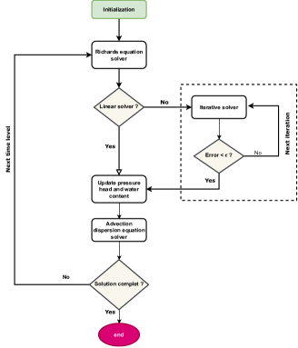
Figure 1: Flowchart diagram for methodology implementation.

As we mentioned before, Richards’ equation exhibits strong nonlinearity due to the presence of the hydraulic conductivity term and the specific moisture capacity term. Therefore, to address the complexity of Richards’ equation with fully implicit schemes, linearization techniques are essential. Several iterative methods have been employed to linearize the equation, such as the Newton method, Picard method, and L-scheme method, among others [1, 15, 39, 40, 43]. These techniques play a crucial role in making the solution to the equation more tractable and efficient. Several studies have extensively examined these linearization methods by comparing them with each other and adapting strategies to deal with convergence issues. Understanding the performance and limitations of each method has enabled researchers to propose adaptive strategies that can effectively overcome convergence challenges. For instance, K. Mitra et al. [43] provide a modified L-scheme that combines the L-scheme and the modified Picard methods. List and Radu [39] used the L-scheme/Newton method, which is a combination of the L-scheme method and Newton one, and the results show good performance in terms of robustness and time computation. Within the framework of this study, we employ the methodology of the modified Picard approach to linearize the Richards equation in its mixed form, which is widely used in the literature [15, 30, 39]. The modified Picard method utilizes Taylor series expansion to approximate the current iteration level of saturation $S^{n+1,m+1}$ [15], so that,

$$S^{n+1,m+1}=S^{n+1,m}+\dot{S}^{n+1,m}\left(\Psi^{n+1,m+1}-\Psi^{n+1,m}\right)+o\left(\Psi^{n+1,m+1}-\Psi^{n+1,m}\right).$$ (3.15)

The Newton method exhibits quadratic convergence, while the modified Picard method demonstrates linear convergence. Although Newton’s advantageous convergence properties, it requires an initial guess that is so close to the solution to achieve this convergence. The modified Picard method is easy to implement and demands less memory compared to Newton’s method. In each iteration, we start the process by initializing from the previous time step. In other words, $\Psi^{n+1,0}$ is set equal to $\Psi^{n}$. To stop the iteration process, many studies have utilized different stopping criterion expressions [15, 16, 30, 39]. Within the scope of this study, we will use the following criterion:

$$||\Psi^{n+1,m+1}-\Psi^{n+1,m}||_{L^{2}}\leq\epsilon,$$ (3.16)

in which $0<\epsilon\ll 1$ is the tolerance parameter and $||\cdot||_{L^{2}}$ represents the L²-norm, which is defined as

$$||u||_{L^{2}}=\left(\int_{\Omega}|u|^{2}\,\mathrm{d}\bm{x}\right)^{\frac{1}{2}},$$ (3.17)

for a given function $u\in L^{2}(\Omega)$.

Remark 3.4

Celia et al. [15] studied the finite element methods for solving the Richards equation and illustrated that they require the use of mass lumping on the time derivative to effectively prevent nonoscillatory solutions. Different forms of mass lumping have been developed for standard and mixed finite element methods to model infiltration in porous media [7, 15, 66]. In our study, the mass lumping technique used in [15] is applied for the system of Richards equation and the solute transport equation.

Remark 3.5

In this study, the coupled system of unsaturated flow and solute transport in porous media is considered a “one-way coupling”system, where the dynamic of water influences the transport process. In this context, the Richards equation for water flow is solved first to obtain the flow field, and then the advection-dispersion equation is solved for the solute transport. The two equations are connected through this sequential process, representing one-way influence of the flow on solute transport as shown in Figure 1.

4 Numerical results

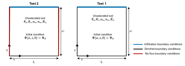
Figure 2: Schematic illustration of the two-dimensional infiltration tests

In this section, we conduct numerical experiments in two-dimensional scenarios, considering both homogeneous and heterogeneous media and employing both the Gardner and the VG models for capillary pressure. Firstly, we will start with a numerical analysis of the studied methods by conducting numerically the convergence rate of the methods (3.10)-(3.13). For the convergence analysis, we will use the $L^{2}$ error as described in (3.17) to calculate the error that occurs between the reference or exact solution and the numerical solution. The rate of convergence, $p$, will be computed using the following formula:

$$p=ln\left(\dfrac{||u-u_{h}||_{L^{2}}}{||u-u_{h/k}||_{L^{2}}}\right)\Big{/}ln\left(k\right),$$ (4.1)

where $u$ represents the reference solution or exact solution, $u_{h}$ represents the numerical solution and $k$ represents the refinement factor between consecutive element sizes or time steps. The value $k=2$ was selected in our numerical tests. Another criterion to test the efficiency of the methods is the CPU time (total runtime). We compare the numerical efficiency of the methods by looking at the CPU time required to reach a desired level of accuracy. Secondly, some application tests will be conducted for the efficient method. We should emphasize that the SILF2 method will be used with the optimal stabilized parameter $\nu=1$ as will be confirmed in the following section. Throughout our analysis, all the numerical tests are performed using an Intel(R) Core(TM) i5-10310U CPU @ 1.70GHz, 2208 Mhz, 4 Core(s), 8 Logical Processor(s) using the finite element platform FreeFem++ [28, 29] with the direct solver UMFPACK [18].

4.1 Numerical tests - Convergence

Here, we focus on the Richards equation as the first step since it is a nonlinear equation and the analysis will be effective to compare the presented methods. To analyze the convergence and efficiency of the proposed methods, we apply them to a variety of infiltration problems and compare them to reference solutions. We consider the following test problems:

1. Two infiltration tests with the Gardner model in homogeneous porous media for which analytical solutions exist [63].

2. One infiltration test with the VG model in heterogeneous porous media for which the reference solution is used.

4.1.1 Green and Ampt infiltration problem

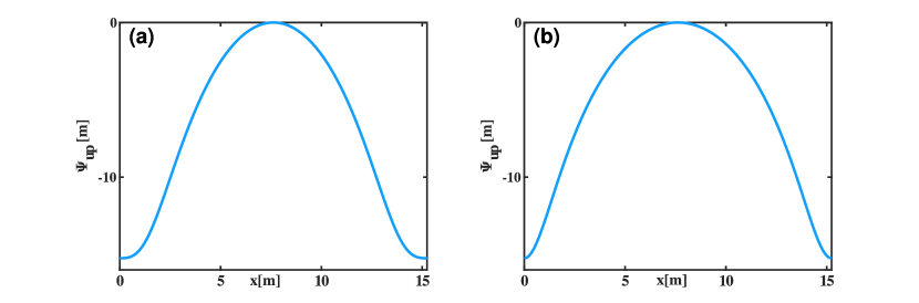
Figure 3: The boundary condition enforced on the top of the soil. (a) and (b) refer to Test 1 and Test 2, respectively.

In this part, the proposed methods will be evaluated using the Gardner model for the capillary pressure. To achieve this, we will leverage analytical solutions from reputable sources in the literature [10, 34, 63]. The capillary rise function and the Leverett $J$-function are expressed as follows:

$$\psi_{c}=\dfrac{1}{\alpha_{v}},\quad\quad J(S)=\log(S).$$ (4.2)

Variable	Symbol	Value
Length of the square domain	$L$ [$m$]	$15.24$
Hydraulic conductivity	$K_{s}$ [$m/day$]	$0.10$
Saturated water content	$\theta_{s}$   [$m^{3}/m^{3}$]	$0.450$
Residual water content	$\theta_{r}$   [$m^{3}/m^{3}$]	$0.150$
Gardner fitting coefficient	$\alpha_{v}$    [$1/m$]	$0.164$
Initial condition	$\Psi_{d}$  [$m$]	$-15.24$
Tolerance criterion	$\epsilon$      [$-$]	$10^{-6}$
Series terms number	$nt$   [$-$]	$200$

Table 1: Parameters and material properties used for 2D infiltration tests

The two numerical tests are performed using the Green and Ampt problem [65] with different boundary conditions. The initial soil is set extremely dry ($\Psi=-15.24\,m$). In Figure 2a and 2b, we depict the precise top boundary condition that defines the soil infiltration procedure. For simplicity, we will refer to the two tests as Test 1 for the first test problem and Test 2 for the second test problem. As illustrated in Figure 2, the boundary conditions of Test 1 and Test 2 are expressed in the following formulations:

1. Test 1: Dirichlet boundary conditions are enforced on the four sides:

   $$\left\{\begin{array}[]{ll}\begin{aligned} \Psi(x,z,t=0)&=\Psi(x,z=0,t)=\Psi(x=0,z,t)=\Psi(x=L,z,t)=\Psi_{d},\\ \Psi(x,z=L,t)&=\Psi_{up}(x)=\frac{1}{\alpha_{v}}\log\left(\zeta+\left(1-\zeta\right)\left[\frac{3}{4}\sin\left(\frac{\pi x}{L}\right)-\frac{1}{4}\sin\left(\frac{3\pi x}{L}\right)\right]\right).\end{aligned}\end{array}\right.$$ (4.3)

2. Test 2: No flux boundary conditions are enforced on the lateral sides of the domain, while Dirichlet boundary conditions are prescribed at the upper and bottom boundaries:

   $$\left\{\begin{array}[]{ll}\begin{aligned} \Psi(x,z,t=0)&=\Psi(x=0,z,t)=\Psi_{d},\\ \Psi(x,z=L,t)&=\Psi_{up}(x)=\frac{1}{\alpha_{v}}\log\left[\zeta+\frac{\left(1-\zeta\right)}{2}(1-\cos\left(\frac{2\pi x}{L}\right)\right],\end{aligned}\end{array}\right.$$ (4.4)

where $\Psi_{up}(x)$ is a function that depends on $x$ and is described as the top boundary condition of the two tests. The two-dimensional analytical solutions of the Richards equation related to these tests are expressed as follows: [10, 34, 63]:

$$\Psi(x,z,t)=\psi_{c}\log(\zeta+\Psi_{0}(x,z,t)),$$ (4.5)

where $\Psi_{0}(x,z,t)$ is given for each test by the following expressions:
Test 1:

$$\left\{\begin{array}[]{ll}\begin{aligned} &\Psi_{0}(x,z,t)=(1-\zeta)\exp(\frac{\alpha_{v}}{2}(L-z))\bigg{(}\dfrac{3}{4}\sin(\dfrac{\pi x}{L})\bigg{[}\dfrac{\sinh(\beta_{1}z)}{\sinh(\beta_{1}L)}+\dfrac{2}{Ld}\sum_{p=1}^{\infty}(-1)^{{}^{p}}\dfrac{\lambda_{p}}{\nu_{1p}}\sin(\lambda_{p}z)\\ &\times\exp(-\nu_{1p}t)\bigg{]}-\dfrac{1}{4}\sin(\dfrac{3\pi x}{L})\bigg{[}\dfrac{\sinh(\beta_{3}z)}{\sinh(\beta_{3}L)}+\dfrac{2}{Ld}\sum_{p=1}^{\infty}(-1)^{{}^{p}}\dfrac{\lambda_{p}}{\nu_{3p}}\sin(\lambda_{p}z)\exp(-\nu_{3p}t)\bigg{]}\bigg{)}.\end{aligned}\end{array}\right.$$ (4.6)

Test 2:

$$\Psi_{0}(x,z,t)=(1-\zeta)\sin\left(\frac{\pi x}{L}\right)\exp(\frac{\alpha_{v}}{2}(L-z))\bigg{[}\dfrac{\sinh(\beta_{1}z)}{\sinh(\beta_{1}L)}+\dfrac{2}{Ld}\sum_{p=1}^{\infty}(-1)^{{}^{p}}\dfrac{\lambda_{p}}{\nu_{1p}}\sin(\lambda_{p}z)\times\exp(-\nu_{1p}t)\bigg{]}$$ (4.7)

with

$$\zeta=\exp(\alpha_{v}\Psi_{d}),\;d=\dfrac{\alpha_{v}\phi}{K_{s}},\;\lambda_{p}=\dfrac{\pi p}{L},\;\beta_{i}=\Big{(}\frac{\alpha_{v}^{2}}{4}+(\frac{i\pi}{L})^{2}\Big{)}^{\frac{1}{2}},\;\text{and}\;\nu_{ip}=\dfrac{\beta_{i}^{2}+\lambda_{p}^{2}}{d}\quad.$$ (4.8)

We numerically solved the Richards equation in the square domain $\Omega=[0,L]\times[0,L]$ shown in Figure 2 using the studied numerical methods. The parameters and soil proprieties used in the numerical tests are depicted in Table 1 [10, 34].

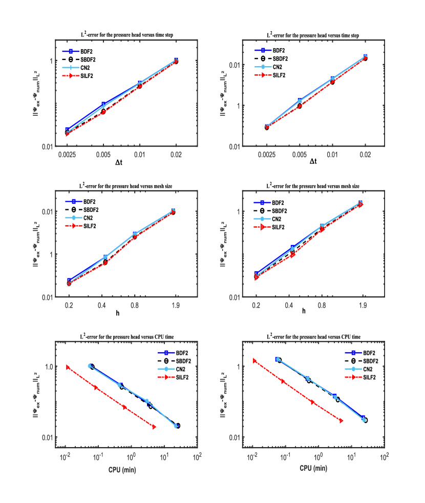
Figure 4: $L^{2}$ error on log-scaled of the pressure head for Test 1 (left column) and Test 2 (right column) as a function of time step (top), mesh size (middle), and CPU time (bottom) for all proposed methods.

Table 2: $L^{2}$-error for Test 1 and Test 2 using the SILF2 method with different values of the free parameter $\nu$.

Parameter $\nu$	$L^{2}$-error for Test 1		$L^{2}$-error for Test 2
	On $\Psi_{h}$	On $S_{h}$	On $\Psi_{h}$	On $S_{h}$
0.6	0.956876	0.0248646	1.46798	0.0396786
0.7	0.944442	0.0243397	1.44387	0.0390766
0.8	0.941243	0.0240901	1.43433	0.0387697
0.9	0.941676	0.0240025	1.43430	0.0386571
1.0	0.940499	0.0239274	1.43371	0.0386333

In the numerical analysis, we opt to study the $L^{2}$-error versus time step, versus mesh size, and versus CPU time for a final time $T=5$ days with a varying time step of $\Delta t=0.02,\,0.01,\,0.005,\,0.0025$ and mesh size of $h=1.9,\,0.8,\,0.4,\,0.2$, where the subdivisions $12\times 12,\,25\times 25,\,50\times 50$ and $100\times 100$ along the boundaries of the domain are used respectively. A suitable tolerance criterion was selected to ensure the convergence of the iterative technique and the accuracy of the methods. However, this can lead to some observed computational overhead regarding CPU time. Figure 4 depicts the $L^{2}$-error values of the pressure head obtained with varying $\Delta t,\,h$ and CPU for both two tests. We analyze the SILF2 method using different values of the free parameter $\nu$ to ensure both stability and accuracy. As shown in Table 2, the optimal value of the free parameter is $\nu=1$. The SILF2 method with this optimal free parameter is the most accurate scheme, followed by the SBDF2 method. Regarding the computational time, the SILF2 method leads to accurate results with less computational cost thanks to its linear nature starting from the second step. In terms of accuracy, all methods are of order $2$ demonstrating a satisfactory agreement with the theoretical analysis presented in Appendix A. Table 3 offers a detailed analysis of $L^{2}$-error, rate of convergence, and CUP time of the BDF2, SBDF2, CN2, and SILF2 methods. The comparison between the spatial distribution of the saturation for the numerical and analytical solutions at the final time $T=5$ days for both tests is illustrated in Figure 5. For the numerical solution, we utilized a mesh size of $h=0.4$ ($50\times 50$) and a time step of $\Delta t=0.005$. The contour plots showcase good agreement between the numerical and analytical solutions.

Table 3: $L^{2}$-error, order of convergence and CPU time as a function of mesh size and time step of the studied methods for the two numerical tests.

Method	$h$	$\Delta t$	Test 1			Test 2
			$L^{2}$-error	Order	CPU (s)	$L^{2}$-error	Order	CPU (s)
BDF2	1.9	2E-2	1.02326		3.62	1.57566		3.32
	0.8	1E-2	0.2982		29.13	0.44962		27.36
	0.4	5E-3	0.095769		201.89	0.144199		184.95
	0.2	2.5E-3	0.0243305	$1.97$	1460.54	0.03518	$2.03$	1351.67
SBDF2	1.9	2E-2	0.956127		3.96	1.4757		3.96
	0.8	1E-2	0.262932		30.55	0.396407		30.63
	0.4	5E-3	0.0742976		230.88	0.114618		230.54
	0.2	2.5E-3	0.0208178	$1.84$	1564.93	0.0297928	$1.94$	1600.08
CN2	1.9	2E-2	1.02183		3.27	1.57495		3.52
	0.8	1E-2	0.295176		26	0.453597		28.32
	0.4	5E-3	0.103785		176.77	0.132803		194.94
	0.2	2.5E-3	0.0206168	$2.09$	1322.78	0.0301976	$2.1$	1440.91
SILF2	1.9	2E-2	0.940499		0.69	1.43371		0.67
	0.8	1E-2	0.250411		4.96	0.376912		4.89
	0.4	5E-3	0.0696979		36.86	0.0968422		39.02
	0.2	2.5E-3	0.0193712	$1.85$	287.72	0.0289613	$1.86$	286.7

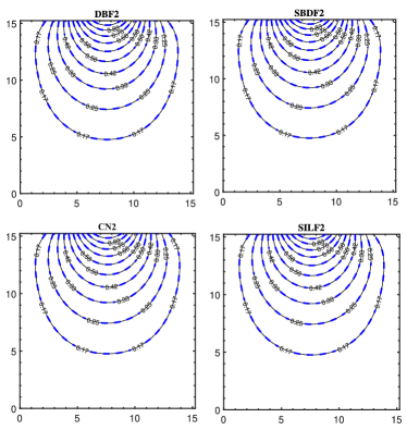
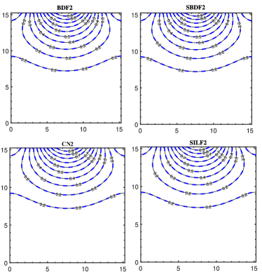
Figure 5: Numerical results for Test 1 (left) and Test 2 (right). Comparison between numerical solution ( ) using BDF2, SBDF2, CN2 and SILF2 methods and exact solution ( ) for the saturation.

Figure 6: Total mass analysis for Test 1 (left) and Test 2 (right). (a) and (b) represent the total mass evolution over time of the numerical and exact solutions. (c) and (d) represent the relative mass balance errors of the numerical methods at discrete times $t=7.2$ min, $t=1$ day, $t=2$ days, $\cdots$, $t=9$ days.

In the following, we compare the total mass evolution for the numerical and exact solutions using the following terms:

$$\int_{\Omega}\theta(\bm{x},t)\,\mathrm{d}\bm{x}\quad\text{and}\quad\int_{\Omega}\theta_{ex}(\bm{x},t)\,\mathrm{d}\bm{x},$$ (4.9)

where $\theta$ and $\theta_{ex}$ represent the numerical and exact solutions of the moisture content, respectively. For all the studied methods, we computed the relative mass balance error (MBE) at each time level using the following formulae [15, 50]:

$$\text{MBE}(t)=\Bigg{|}1-\dfrac{\text{MB}_{num}(t)}{\text{MB}_{ex}(t)}\Bigg{|}\times 100,$$ (4.10)

where $\text{MB}_{num}(t)=\int_{\Omega}\left[\theta(\bm{x},t)-\theta_{0}(\bm{x})\right]\,\mathrm{d}\bm{x}$ and $\text{MB}_{ex}(t)=\int_{\Omega}\left[\theta_{ex}(\bm{x},t)-\theta_{0}(\bm{x})\right]\,\mathrm{d}\bm{x}$ represent the total mass change that occurs in the domain $\Omega$ within the time period for the numerical and exact solutions, and $\theta_{0}(\bm{x}):=\theta(\bm{x},t=0)$ is the initial moisture content. We consider the mesh size $h=0.8$ where a total of 5000 triangles and 2601 vertices are used, the time step $\Delta t=0.005$ and the final time $T=10$ days. Figure 6a and 6c depict the resulting mass evolution for the numerical and exact solutions for Test 1 and Test 2, respectively. The results demonstrate good agreement between the numerical mass evolution and the exact one for both tests. Figure 6b and 6d illustrate the corresponding relative mass balance error for Test 1 and Test 2, respectively. The results indicate a mass error at the beginning of the evolution, which diminishes rapidly as the period of evolution extends.

4.1.2 Heterogeneous soil test

The previous part related to 2D homogeneous soils confirmed that the SILF2 method is accurate and it requires a small CPU time. In this part, we aim to test the efficiency and performance of this method in two-dimensional heterogeneous soil. The VG model is used to describe the relation between the saturation, the pressure head and the hydraulic conductivity. The capillary rise and the Leverett $J$-function are given by:

$$\psi_{c}=\dfrac{1}{\alpha_{v}},\quad\quad J(S)=-\big{[}S^{-\frac{1}{m_{v}}}-1\big{]}^{\frac{1}{n_{v}}}.$$ (4.11)

A square computational domain with a length of $100\;cm$ is separated into two sub-regions by an L-shape form as illustrated in Figure 7. We consider the initial condition $\Psi(x,z,t=0)=-z$. Homogeneous Dirichlet boundary conditions are used at the top and bottom boundaries, while homogeneous Neumann boundary conditions are imposed at the lateral sides.

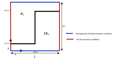
Figure 7: Schematic illustration of the L-shape domain separated into two sub-regions.

Material propriety	Symbol	value
Saturated hydraulic conductivity	$K_{s}$[$cm/s$]	$6.944E-5$
Saturated water content	$\theta_{s}$ [$cm^{3}/cm^{3}$]	$0.5$
Residual water content	$\theta_{r}$ [$cm^{3}/cm^{3}$]	$0.12$
VG fitting coefficient	$\alpha_{v}$ [$1/cm$]	$0.02$
VG parameter	$n_{v}$[$-$]	$3$

Table 4: Material properties used for the heterogeneous test

This test was carried out in [5], where the two-layered soils of the domain are considered to have the same features except the saturated hydraulic conductivity. The first soil has a saturated hydraulic conductivity $K_{s}$, while the second has a saturated hydraulic conductivity equal to $3K_{s}$ as illustrated in Figure 7. The material properties related to this test are given in Table 4. The domain is discretized with a nonuniform triangular mesh with a mesh size of $h=1\,cm$ where a total of 93234 elements and 47045 vertices are used. The time step $\Delta t=\frac{1}{180}$ hour is chosen, and the simulation time is $T=48$ hours. Figure 8 demonstrates the evolution of the saturation in time simulated using the SILF2 scheme and the results agree well with those of the previous studies for this test [5, 11, 34]. Regarding the convergence analysis, a reference solution is computed by discretizing the domain with a total of $1254412$ triangles and $628780$ vertices and with a time step $\Delta t=\frac{1}{360}$ hour. Here, we use the relative $L^{2}$-error, which is given by

$$\frac{\|u_{\text{ref},h}-u_{h}\|_{L^{2}}}{\|u_{\text{ref},h}\|_{L^{2}}},$$ (4.12)

where $u_{\text{ref},h}$ and $u_{h}$ represent the numerical and reference solutions , respectively. Table 5 displays the relative $L^{2}$-errors for both the pressure head and saturation as well as the CPU time in function of the varying time step. An order of convergence around $1.63$ is observed for the pressure head.

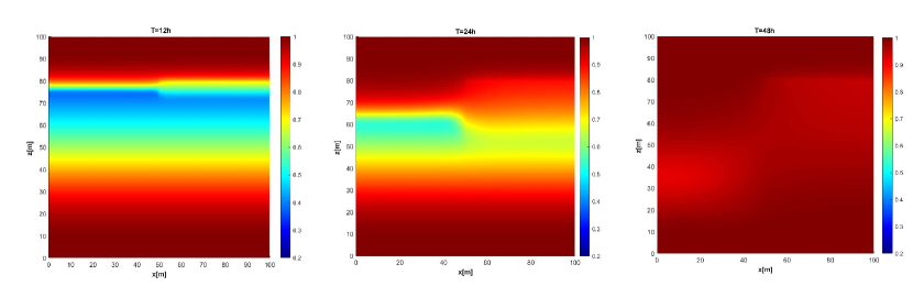
Figure 8: Time evolution of the saturation using SILF2 scheme for the heterogeneous test.

Table 5: Relative $L^{2}$-error and CPU time as a function of time step using the SILF2 method for the heterogeneous soil test.

$\Delta t$(s)	Relative $L^{2}$-error on $\Psi_{h}$	Relative $L^{2}$-error on $S_{h}$	CPU(s)
$160$	0.183642	0.083599	5041.71
$80$	0.13213	0.0502052	5888.65
$40$	0.0831433	0.0223597	10035.9
$20$	0.0524077	0.00721635	12056

In the following, we will focus on application tests including solute transport through unsaturated soils where we consider:

1. 2D numerical test to model water flow and soil salt transport in a loamy soil [25].

2. 2D numerical test to model nitrate transport under surface drip fertigation [37].

4.2 Soil salt transport

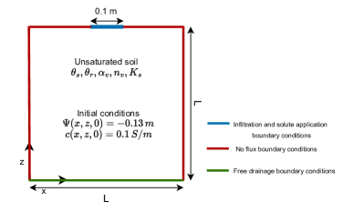
Figure 9: Schematic illustration of the soil salt transport test.

In this test, we will examine the proposed numerical approach for modeling water flow and soil salt transport through unsaturated porous media. Haruzi and Moreno [25] investigate the infiltration and redistribution of water and soil salt transport in a loamy soil using a physical-information neural network approach. As the authors described in [25], the soil salt concentration is determined by calculating the pore-water electrical conductivity (EC). The data used in this study is provided by the authors and it is available in [26]. We will use the provided Hydrus simulations to compare them with the numerical results obtained using the proposed SILF2 scheme. A square computational domain with a length $L=2\,m$ is used. At the center of the top boundary, a section with a width of $10\,cm$ is considered to infiltrate the water using a rate of $0.1\,m/day$. The initial pressure head condition is equal to $-0.13\,m$. Free drainage is enforced at the bottom of the domain. The remaining boundaries are considered to have no water flux. Regarding the solute transport, the initial concentration condition is equal to $0.1\,S/m$. A third type of boundary condition (Cauchy boundary conditions) is applied in the section at the top boundary, involving a constant inflow of solute where the inflow of water is considered with constant concentration $c=1\,S/m$. The VG model is used for the capillary pressure. Figure 9 summarizes the prescribed geometry and boundary conditions, while Table 6 provides parameters and material proprieties related to the test problem. The domain is discretized using an unstructured triangular mesh with a mesh size of 0.061 where a total of 19270 triangles, 9869 vertices, and 50 nodes on each side of the square domain are used. We consider a time step $\Delta t=10^{-3}$ and the simulation time is $T=1\,day$. Figure 10a and 10b illustrate the evolution of the pressure head and solute transport with time, respectively. Good agreements are obtained between the results of the SILF2 method and those obtained in [25]. For a more details comparison, we make a vertical cross-section at the center of the domain ($x=0$) for the pressure head and solute concentration solutions. The resulting 1D solutions are depicted in Figure 11 demonstrating good agreement between our results and those in [25].

Material propriety	Symbol	value
Saturated hydraulic conductivity	$K_{s}$ [$m/day$]	$0.25$
Saturated water content	$\theta_{s}$ [$m^{3}/m^{3}$]	$0.43$
Residual water content	$\theta_{r}$ [$m^{3}/m^{3}$]	$0.078$
VG fitting coefficient	$\alpha_{v}$ [$1/m$]	$3.6$
VG parameter	$n_{v}$ [$-$]	$1.56$
Molecular diffusion coefficient	$\lambda_{m}$ [$m^{2}/day$]	$0.0$
Longitudinal dispersivity	$\lambda_{L}$ [$m$]	$0.5$
Transversal dispersivity	$\lambda_{T}$ [$m$]	$0.1$

Table 6: Material proprieties used for the soil salt transport test [25].

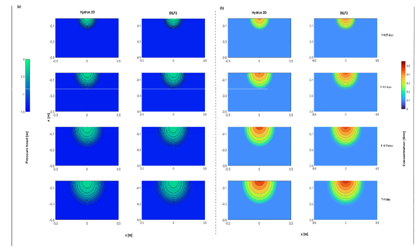
Figure 10: Time evolution of the pressure head (a) and the salt soil transport (b) using SILF2 method compared to the Hydrus simulations in [26].

Figure 11: Pressure head (a) and soil salt transport (b) vertical cross-section ($x=0$). SILF2 scheme compared to the Hydrus simulations in [26].

4.3 Nitrate transport

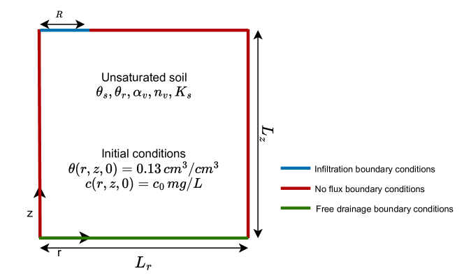
Figure 12: Schematic illustration of the domain for the nitrate transport test.

Further numerical investigation will be carried out to test the performance of the proposed methodology for modeling water flow and nitrate transport under surface drip fertigation. Li et al. 2005 [37] incorporate the presented test problem to compare numerical results with the laboratory data obtained from studies in [38]. The experiment was conducted in a cylinder where the infiltration and nitrate transport processes are considered axisymmetrical, emphasizing the radius ($r$) and depth ($z$) as variables in the analysis. Thanks to the axisymmetrical nature of the problem, a rectangular computational domain of length $L_{r}=41\,cm$ and width $L_{z}=40\,cm$ is considered and a water entry zone of radius $R$ is located at the left of the top boundary as shown in Figure 12. In [37], the authors investigate the impact of different fertigation strategies on water movement and nitrogen dynamics in the soil by applying ammonium nitrate fertilizer ($NH_{4}NO_{3}$) from the saturated entry zone. The VG model is used for the capillary pressure. The initial water content and nitrate concentration were distributed uniformly in the domain, that is, $\theta(r,z,0)=0.13\,cm^{3}/cm^{3}$ and $c(r,z,0)=247.5\,mg/L$. For the VG model, the capillary pressure is 0 in the saturated entry zone, and since the pounded water depth at the saturated entry zone is about $0.15\,cm$, the hydrostatic pressure will be added, i.e. $\Psi=0.15\,cm$. The boundary conditions for this test are expressed as follows:

• Dirichlet boundary conditions for the pressure head and nitrate concentration are imposed at the surface saturated entry zone:

  $$\left\{\begin{array}[]{ll}\begin{aligned} \Psi(r,L_{z},t)&=0.15\;cm&0\leq r\leq R,\\ c(r,L_{z},t)&=C_{a}\;mg/L&0\leq r\leq R.\end{aligned}\end{array}\right.$$ (4.13)

• No flux boundary conditions for water flow are applied to the top boundary of the domain outside of the surface saturated entry zone:

  $$-K\Big{[}\dfrac{\partial\Psi}{\partial r}+1\Big{]}=0\quad R\leq r\leq L_{r},z=L_{z}.$$

• No-flux boundary conditions for water flow and nitrate concentration are enforced in the lateral sides of the domain:

  $$\left\{\begin{array}[]{ll}\begin{aligned} -K\dfrac{\partial\Psi}{\partial r}=0\quad&r=0,\;r=L_{r},\;0\leq z\leq L_{z},\\ \\ \theta D_{rr}\dfrac{\partial c}{\partial r}=0\quad&r=0,\;r=L_{r},\;0\leq z\leq L_{z}.\end{aligned}\end{array}\right.$$ (4.14)

• Free drainage boundary conditions are used in the bottom of the domain:

  $$\left\{\begin{array}[]{ll}\begin{aligned} \dfrac{\partial\Psi}{\partial z}=0\quad&z=0,\;0\leq r\leq L_{r},\\ \\ \theta D_{zz}\dfrac{\partial c}{\partial z}=0\quad&z=0,\;0\leq r\leq L_{r}.\qquad\qquad\quad\end{aligned}\end{array}\right.$$ (4.15)

Material propriety	Symbol	value
Radius of the entry zone	$R$ [$cm$]	$5.6$
Saturated hydraulic conductivity	$K_{s}$ [$cm/hour$]	$1.96$
Saturated water content	$\theta_{s}$ [$cm^{3}/cm^{3}$]	$0.41$
Residual water content	$\theta_{r}$ [$cm^{3}/cm^{3}$]	$0.047$
VG fitting coefficient	$\alpha_{v}$ [$1/cm$]	$0.015$
VG parameter	$n_{v}$ [$-$]	$1.48$
Molecular diffusion coefficient	$\lambda_{m}$ [$cm^{2}/min$]	$0.0015$
Longitudinal dispersivity	$\lambda_{L}$ [$cm$]	$0.32$
Transversal dispersivity	$\lambda_{L}$ [$cm$]	$0.0032$

Table 7: Parameters and material proprieties used for nitrate transport under surface drip fertigation [37].

Parameters and material properties related to the test problem are listed in Table 7. In [37], $NH_{4}NO_{3}$ fertilizer is applied, where mineralization and some reactions are neglected. The adsorption process between the solid phase of the soil and nitrate is also neglected. Regarding the numerical method, the domain geometry is discretized by an unstructured mesh with a total of 3153 non-uniform triangles and 1651 vertices and a time step $\Delta t=10^{-4}$ is used. The water movement and nitrate transport in the domain are simulated at the final time $T=8$ hours. Figure 13 depicts the comparison of the simulated and experimental water content using cross-section profiles. Vertical cross-sections are fixed at $r=2.5\,cm$ and $r=12.5\,cm$, while horizontal cross-sections are fixed at $z=2.5\,cm$ and $z=12.5\,cm$. Furthermore, Figure 14 illustrates vertical cross-section profiles, fixed at $r=2.5\,cm$ and $r=12.5\,cm$, of the nitrate concentration for various input concentrations $C_{a}$ of $NO_{3}^{-}$ as a function of depth. The numerical results obtained using the SILF2 method are in good agreement with the observed data.

Figure 13: Comparison of the observed and simulated water content for the nitrate transport test.

In [37], the authors suggested three different strategies for drip fertigation of nitrate in the soil to evaluate the water and nitrate use efficiency:

• Strategy (A): Apply water and $NH_{4}NO_{3}$ at the beginning for $1/2$ of the total irrigation duration, followed by continued application of water for the remaining time of irrigation.

• Strategy (B): Apply water, firstly, for $1/4$ of the total irrigation duration, then apply $NH_{4}NO_{3}$ for $1/2$ of the total irrigation duration, followed by continued application of water for the remaining $1/4$ of the total time irrigation.

• Strategy (C): Apply water, firstly, for $1/8$ of the total irrigation time, then apply $NH_{4}NO_{3}$ for $1/2$ of the total irrigation duration, followed by continued application of water for the remaining $3/4$ of the total time irrigation.

Throughout the studies, the authors demonstrate that Strategy (B) is recommended as the optimal fertigation strategy. We will evaluate the proposed SILF2 method in addressing the simulation of these three strategies. The discretization of the domain, the time step, and the initial water content are preserved as in the previous test, while the initial concentration of the nitrate is assigned the value $0\,mg/L$. The spatial distribution of water content and nitrate concentration for the three strategies at the time $T=6$ hours are illustrated in Figure 15. Additionally, Figure 15 depicts vertical cross-section profiles, with $r=2.5\,cm$ and $r=12.5\,cm$, of nitrate concentration. We obtained good agreement between the numerical results of the SILF2 method and those presented in [37].

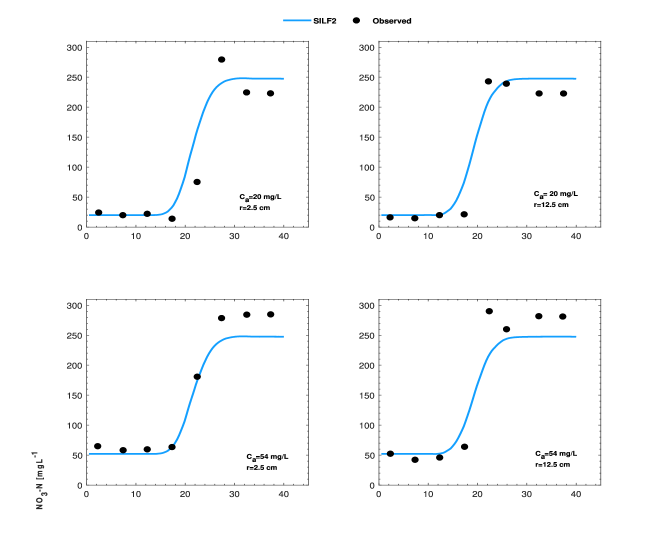
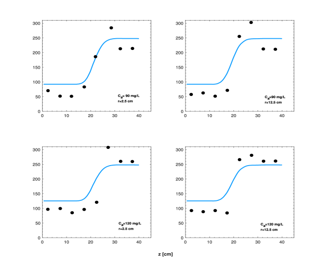
Figure 14: Comparison between the simulated and observed results of the nitrate concentration using different inputs of nitrate concentration.

Figure 15: Water content (top) and nitrate (down) distributions after 6 hours of fertigation for the three strategies using the SILF2 method.

5 Conclusion

The present study focuses on second-order temporal schemes for modeling infiltration and solute transport in unsaturated porous media. The spatial discretization is based on the standard finite element method and two categories of the proposed time-stepping schemes are used. The first category includes BDF2, SBDF2 and CN2 methods, which require an iterative process to solve the Richards equation. The second category is represented by the developed SILF2 method which includes a free stabilized parameter without using any iterative process to solve the system of equations.

The accuracy and efficiency of these schemes are studied using numerical tests for modeling infiltration in soils for which reference solutions are available. The results demonstrate that the SILF2 method with the optimal free parameter $\nu=1$ is accurate and yields better results than the other methods in terms of efficiency and computational cost. Furthermore, the performance and robustness of the SILF2 method are evaluated by two numerical tests involving infiltration and solute transport processes. The first test describes the infiltration and soil salt transport through a homogeneous porous medium. The second one describes the nitrate transport under surface drip fertigation where we used laboratory experimental data for comparison. The results show the capability of the SILF2 method using a semi-implicit technique in time and the standard finite element method in space to simulate infiltration and solute transport processes.

Declaration of competing interest

The authors affirm that they do not have any known financial interests or personal relationships that could be perceived to have influenced the work presented in this paper.

Acknowledgments

Funding for this research was provided by UM6P/OCP Group of Morocco, the Moroccan Ministry of Higher Education, Scientific Research and Innovation and the OCP Foundation (APRD research program), and Natural Sciences and Engineering Research Council of Canada.

All the numerical tests presented in this study were conducted using the supercomputer simlab-cluster, supported by University Mohammed VI Polytechnic, and facilities of simlab-cluster HPC $\&$ IA platform.

Appendix Appendix A Truncation error

To demonstrate the second-order convergence of the proposed numerical schemes, we consider the following equation:

$$\dfrac{\partial\varphi}{\partial t}=F\left(\varphi,t\right),$$ (Appendix A.1)

with the following temporal discretization:

$$\dfrac{[\![\varphi(t_{n+\delta})]\!]}{\Delta t}=\Big{[}A(\varphi(t_{n+\delta})\Big{]},$$ (Appendix A.2)

where

$$\left[\!\left[\varphi(t_{n+\delta})\right]\!\right] =\left(\frac{1}{2}+\delta\right)\varphi\left(t_{n+1}\right)-2\delta\varphi(t_{n})+\left(\delta-\frac{1}{2}\right)\varphi(t_{n-1}),$$ (Appendix A.3)

$$\Big{[}A(\varphi(t_{n+\delta})\Big{]} =\left(\delta+\mu\right)F\big{(}\varphi(t_{n+1})\big{)}+\left(1-\delta-2\mu\right)F\big{(}\varphi(t_{n})\big{)}+\mu F\big{(}\varphi(t_{n-1})\big{)}.$$

By employing the Taylor series expansion and with the assumption of sufficient smoothness, the terms within equation (Appendix A.3) can be centered about the current time level $t_{n+\delta}$ as follows:

$$\dfrac{[\![\varphi(t_{n+\delta})]\!]}{\Delta t}=\dfrac{\partial\varphi}{\partial t}(t_{n+\delta})+\frac{\Delta t^{2}}{6}\left[(1-\delta)^{3}\Big{(}\delta+\frac{1}{2}\Big{)}+2\delta^{4}-(1+\delta)^{3}\Big{(}\delta-\frac{1}{2}\Big{)}\right]\frac{\partial^{3}\varphi}{\partial t^{3}}(t_{n+\delta})+O(\Delta t^{3}),$$ (Appendix A.4)

$$\Big{[}A(\varphi(t_{n+\delta})\Big{]}=F(\varphi(t_{n+\delta}))+(\delta+\mu)\bigg{[}\Big{(}\varphi(t_{n+1})-\varphi(t_{n+\delta})\Big{)}F^{\prime}(\varphi(t_{n+\delta}))+\dfrac{\left(\varphi(t_{n+1})-\varphi(t_{n+\delta})\right)^{2}}{2}F^{\prime\prime}(\varphi(t_{n+\delta}))\bigg{]}$$

$$\qquad\qquad\;\quad+(1-\delta-2\mu)\bigg{[}\Big{(}\varphi(t_{n})-\varphi(t_{n+\delta})\Big{)}F^{\prime}(\varphi(t_{n+\delta}))+\dfrac{(\varphi(t_{n})-\varphi(t_{n+\delta}))^{2}}{2}F^{\prime\prime}(\varphi(t_{n+\delta}))\bigg{]}$$

$$\qquad\qquad\;\quad+\mu\bigg{[}\Big{(}\varphi(t_{n-1})-\varphi(t_{n+\delta})\Big{)}F^{\prime}(\varphi(t_{n+\delta}))+\dfrac{(\varphi(t_{n-1})-\varphi(t_{n+\delta}))^{2}}{2}F^{\prime\prime}(\varphi(t_{n+\delta}))\bigg{]}$$

$$\qquad\qquad\;\quad+O\left(\Delta_{n+1-\delta}^{3}\right)+O\left(\Delta_{n+\delta}^{3}\right)+O\left(\Delta_{n-1-\delta}^{3}\right),$$

where $\Delta_{n+1-\delta}=\varphi(t_{n+1})-\varphi(t_{n+\delta})$, $\Delta_{n+\delta}=\varphi(t_{n})-\varphi(t_{n+\delta})$ and $\Delta_{n-1-\delta}=\varphi(t_{n-1})-\varphi(t_{n+\delta})$.

Using the Taylor series, the term $\varphi(t_{n+1})$ is approximated around the time level $t_{n+\delta}$ as follows:

$$\varphi(t_{n+1})=\varphi(t_{n+\delta})+\Delta t(1-\delta)\dfrac{\partial\varphi}{\partial t}\left(t_{n+\delta}\right)+\dfrac{\Delta t^{2}(1-\delta)^{2}}{2}\dfrac{\partial^{2}\varphi}{\partial t^{2}}\left(t_{n+\delta}\right)+O(\Delta t^{3}).$$ (Appendix A.5)

By utilizing the same calculations to expand $\varphi(t_{n})$ and $\varphi(t_{n-1})$ around the time level $t_{n+\delta}$, we get

$$\Big{[}A(\varphi(t_{n+\delta})\Big{]}=F(\varphi(t_{n+\delta})) +\Delta t^{2}\bigg{[}\dfrac{(\delta+\mu)(1-\delta)^{2}}{2}+\dfrac{(1-\delta-2\mu)\delta^{2}}{2}+\dfrac{\mu(1+\delta)^{2}}{2}\bigg{]}$$ (Appendix A.6)

$$\times\Big{(}F^{\prime}(\varphi(t_{n+\delta}))+F^{\prime\prime}(\varphi(t_{n+\delta}))\Big{)}+O(\Delta t^{3}).$$

We conclude that the scheme (Appendix A.2) exhibits a second-order truncation error. Consequently, BDF2, SBDF2 and CN2 schemes are of second order accuracy.

Regarding the SILF2 method presented in (3.13), we will use the following notations:

$$\!] =\dfrac{\Psi_{h}(t_{n+1})-\Psi_{h}(t_{n-1})}{2\Delta t},$$ (Appendix A.7)

$$[\![R_{h}(t_{n})]\!]_{\nu} =\nu\Psi_{h}(t_{n+1})+(1-2\nu)\Psi_{h}(t_{n})+\nu\Psi_{h}(t_{n-1}).$$

By employing the Taylor series to expand the terms in (Appendix A.7), we obtain:

$$[\![\Psi_{h}(t_{n})]\!]=\dfrac{\partial\Psi_{h}}{\partial t}(t_{n})+\left(\dfrac{\Delta t^{2}}{6}\right)\frac{\partial^{3}\Psi_{h}}{\partial t^{3}}(t_{n})+O(\Delta t^{3}),$$ (Appendix A.8)

$$\qquad\qquad\;=\dfrac{\partial\Psi}{\partial t}(t_{n})+O(\Delta t^{2}),$$

$$[\![R_{h}(t_{n})]\!]_{\nu}=\Psi_{h}(t_{n})+\Delta t^{2}\frac{\partial^{2}\Psi_{h}}{\partial t^{2}}(t_{n})+O(\Delta t^{3}).$$

We conclude that the SILF2 method exhibits a second-order truncation error.

References

- Albuja and Ávila, [2021] Albuja, G. and Ávila, A. I. (2021). A family of new globally convergent linearization schemes for solving Richards’ equation. Applied Numerical Mathematics, 159:281–296.
- Alt and Luckhaus, [1983] Alt, H. W. and Luckhaus, S. (1983). Quasilinear elliptic-parabolic differential equations. Math. Z, 183(3):311–341.
- Antonietti et al., [2019] Antonietti, P. F., Facciola, C., Russo, A., and Verani, M. (2019). Discontinuous Galerkin approximation of flows in fractured porous media on polytopic grids. SIAM Journal on Scientific Computing, 41(1):A109–A138.
- Ascher et al., [1995] Ascher, U. M., Ruuth, S. J., and Wetton, B. T. (1995). Implicit-explicit methods for time-dependent partial differential equations. SIAM Journal on Numerical Analysis, 32(3):797–823.
- Baron et al., [2017] Baron, V., Coudière, Y., and Sochala, P. (2017). Adaptive multistep time discretization and linearization based on a posteriori error estimates for the Richards equation. Applied Numerical Mathematics, 112:104–125.
- Bear, [2013] Bear, J. (2013). Dynamics of fluids in porous media. Courier Corporation.
- Belfort et al., [2009] Belfort, B., Ramasomanana, F., Younes, A., and Lehmann, F. (2009). An efficient lumped mixed hybrid finite element formulation for variably saturated groundwater flow. Vadose Zone Journal, 8:352–362.
- Beljadid et al., [2020] Beljadid, A., Cueto-Felgueroso, L., and Juanes, R. (2020). A continuum model of unstable infiltration in porous media endowed with an entropy function. Advances in Water Resources, 144:103684.
- Beljadid et al., [2014] Beljadid, A., Mohammadian, A., Charron, M., and Girard, C. (2014). Theoretical and numerical analysis of a class of semi-implicit semi-lagrangian schemes potentially applicable to atmospheric models. Monthly Weather Review, 142:4458–4476.
- Boujoudar et al., [2021] Boujoudar, M., Beljadid, A., and Taik, A. (2021). Localized MQ-RBF meshless techniques for modeling unsaturated flow. Engineering Analysis with Boundary Elements, 130:109–123.
- Boujoudar et al., [2023] Boujoudar, M., Beljadid, A., and Taik, A. (2023). Localized RBF methods for modeling infiltration using the Kirchhoff-transformed Richards equation. Engineering Analysis with Boundary Elements, 152:259–276.
- Boujoudar et al., [2024] Boujoudar, M., Beljadid, A., and Taik, A. (2024). Implicit EXP-RBF techniques for modeling unsaturated flow through soils with water uptake by plant roots. Applied Numerical Mathematics. Positive review.
- Brooks and Corey, [1966] Brooks, R. and Corey, A. (1966). Properties of porous media affecting fluid flow. Journal of the Irrigation and Drainage Division, American Society of Civil Engineers, 92:61–88.
- Brunner and Simmons, [2012] Brunner, P. and Simmons, C. T. (2012). Hydrogeosphere: a fully integrated, physically based hydrological model. Ground water, 50(2):170–176.
- Celia et al., [1990] Celia, M., Boulouts, E., and Zarba, R. (1990). A general mass-conservative numerical solution for the unsaturated flow equation. Water Resources Research, 26:1483–1496.
- Clément et al., [2021] Clément, J. B., Golay, F., Ersoy, M., and Sous, D. (2021). An adaptive strategy for discontinuous Galerkin simulations of Richards’ equation: Application to multi-materials dam wetting. Advances in Water Resources, 151.
- Damodhara Rao et al., [2006] Damodhara Rao, M., Raghuwanshi, N., and Singh, R. (2006). Development of a physically based 1d-infiltration model for irrigated soils. Agricultural Water Management, 85(1):165–174.
- Davis, [2004] Davis, T. A. (2004). Algorithm 832: UMFPACK V4.3 - An unsymmetric-pattern multifrontal method. ACM Transactions on Mathematical Software, 30(2):196 – 199. Cited by: 1072.
- Durran, [2010] Durran, D. R. (2010). Numerical methods for fluid dynamics: With applications to geophysics, volume 32. Springer Science & Business Media.
- Eymard et al., [1999] Eymard, R., Gutnic, M., and Hilhorst, D. (1999). The finite volume method for Richards equation. Computational Geosciences, 3:259–294.
- Farthing and Ogden, [2017] Farthing, M. W. and Ogden, F. L. (2017). Numerical solution of Richards’ equation: A review of advances and challenges. Soil Science Society of America Journal, 81(6):1257–1269.
- Freeze and Cherry, [1979] Freeze, R. A. and Cherry, J. A. (1979). Groundwater prentice-hall inc. Eaglewood Cliffs, NJ.
- Gardner, [1958] Gardner, W. R. (1958). Some steady state solutions of the unsaturated moisture flow equation with application to evaporation from a water table. Soil Science, 85:228–232.
- Girault and Raviart, [2012] Girault, V. and Raviart, P.-A. (2012). Finite element methods for Navier-Stokes equations: theory and algorithms, volume 5. Springer Science & Business Media.
- [25] Haruzi, P. and Moreno, Z. (2023a). Modeling water flow and solute transport in unsaturated soils using physics-informed neural networks trained with geoelectrical data. Water Resources Research, 59(6).
- [26] Haruzi, P. and Moreno, Z. (2023b). Modeling water flow and solute transport in unsaturated soils using physics-informed neural networks trained with geoelectrical data. https://doi.org/10.5281/zenodo.7558746. [Dataset].
- Haverkamp et al., [1977] Haverkamp, R., Vauclin, M., Touma, J., Wierenga, P., and Vachaud, G. (1977). A comparison of numerical simulation models for one-dimensional infiltration. Soil Science Society of America Journal, 41(2):285–294.
- [28] Hecht, F. (2012a). New development in freefem++. Journal of Numerical Mathematics, 20(3-4):251 – 265. Cited by: 2275; All Open Access, Green Open Access.
- [29] Hecht, F. (2012b). New development in freefem++. J. Numer. Math., 20(3-4):251–265.
- Huang et al., [1996] Huang, K., Mohanty, B., and Van Genuchten, M. T. (1996). A new convergence criterion for the modified Picard iteration method to solve the variably saturated flow equation. Journal of Hydrology, 178(1-4):69–91.
- Hundsdorfer and Verwer, [2003] Hundsdorfer, W. H. and Verwer, J. G. (2003). Numerical solution of time-dependent advection-diffusion-reaction equations, volume 33. Springer.
- Kaluarachchi and Parker, [1988] Kaluarachchi, J. J. and Parker, J. (1988). Finite element model of nitrogen species transformation and transport in the unsaturated zone. Journal of Hydrology, 103(3-4):249–274.
- [33] Keita, S., Beljadid, A., and Bourgault, Y. (2021a). Efficient second-order semi-implicit finite element method for fourth-order nonlinear diffusion equations. Computer Physics Communications, 258:107588.
- [34] Keita, S., Beljadid, A., and Bourgault, Y. (2021b). Implicit and semi-implicit second-order time stepping methods for the Richards equation. Advances in Water Resources, 148.
- Lambert et al., [1991] Lambert, J. D. et al. (1991). Numerical methods for ordinary differential systems, volume 146. Wiley New York.
- Levrett, [1941] Levrett, M. C. (1941). Capillary behavior of porous solids. Trans. AIME, 142:152–169.
- Li et al., [2005] Li, J., Zhang, J., and Rao, M. (2005). Modeling of water flow and nitrate transport under surface drip fertigation. Transactions of the ASAE, 48(2):627–637.
- Li et al., [2003] Li, J., Zhang, J., and Ren, L. (2003). Water and nitrogen distribution as affected by fertigation of ammonium nitrate from a point source. Irrigation Science, 22:19–30.
- List and Radu, [2016] List, F. and Radu, F. A. (2016). A study on iterative methods for solving Richards’ equation. Computational Geosciences, 20:341–353.
- Lott et al., [2012] Lott, P. A., Walker, H. F., Woodward, C. S., and Yang, U. M. (2012). An accelerated Picard method for nonlinear systems related to variably saturated flow. Advances in Water Resources, 38:92–101.
- Manzini and Ferraris, [2004] Manzini, G. and Ferraris, S. (2004). Mass-conservative finite volume methods on 2-D unstructured grid for the Richards’ equation. Adv. Water Resour., 27:1199–1215.
- Millington and Quirk, [1961] Millington, R. and Quirk, J. (1961). Permeability of porous solids. Transactions of the Faraday Society, 57:1200–1207.
- Mitra and Pop, [2019] Mitra, K. and Pop, I. S. (2019). A modified L-scheme to solve nonlinear diffusion problems. Computers and Mathematics with Applications, 77:1722–1738.
- Mualem, [1976] Mualem, Y. (1976). A new model for predicting the hydraulic conductivity of unsaturated porous media. Water Resources Research, pages 513–522.
- Nishikawa, [2019] Nishikawa, H. (2019). On large start-up error of BDF2. Journal of Computational Physics, 392:456–461.
- Philip, [1969] Philip, J. R. (1969). Theory of infiltration. In Advances in hydroscience, volume 5, pages 215–296. Elsevier.
- Pinder and Gray, [2013] Pinder, G. F. and Gray, W. G. (2013). Finite element simulation in surface and subsurface hydrology. Elsevier.
- Potts et al., [2001] Potts, D. M., Zdravković, L., Addenbrooke, T. I., Higgins, K. G., and Kovačević, N. (2001). Finite element analysis in geotechnical engineering: application, volume 2. Thomas Telford London.
- Richards, [1931] Richards, L. A. (1931). Capillary conduction of liquids through porous mediums. Journal of Applied Physics, 1:318–333.
- Romano et al., [1998] Romano, N., Brunone, B., and Santini, A. (1998). Numerical analysis of one-dimensional unsaturated flow in layered soils. Advances in Water Resources, 21(4):315–324.
- Ross, [2003] Ross, P. J. (2003). Modeling soil water and solute transport–fast, simplified numerical solutions. Agronomy Journal, 95:1352–1361.
- Russo, [2012] Russo, D. (2012). Numerical analysis of solute transport in variably saturated bimodal heterogeneous formations with mobile–immobile-porosity. Advances in water resources, 47:31–42.
- Russo, [2002] Russo, G. (2002). Central schemes and systems of balance laws, in “hyperbolic partial differential equations. Theory, Numerics and Applications”, edited by Andreas Meister and Jens Struckmeier, Vieweg, Göttingen.
- Selim and Iskandar, [1981] Selim, H. and Iskandar, I. (1981). Modeling nitrogen transport and transformations in soils: 1. theoretical considerations: 1. Soil Science, 131(4):233–241.
- Simunek and Hopmans, [2009] Simunek, J. and Hopmans, J. W. (2009). Modeling compensated root water and nutrient uptake. Ecological Modelling, 220(4):505–521.
- Simunek et al., [2005] Simunek, J., Van Genuchten, M. T., and Sejna, M. (2005). The HYDRUS-1D software package for simulating the one-dimensional movement of water, heat, and multiple solutes in variably-saturated media. University of California-Riverside Research Reports, 3:1–240.
- Simunek et al., [2006] Simunek, J., van Genuchten, M. T., and Sejna, M. (2006). The HYDRUS software package for simulating two-and three-dimensional movement of water, heat, and multiple solutes in variably-saturated media. Technical manual, version, 1:241.
- Simunek et al., [2016] Simunek, J., Van Genuchten, M. T., and Sejna, M. (2016). Recent developments and applications of the HYDRUS computer software packages. Vadose Zone Journal, 15(7).
- Siyal et al., [2012] Siyal, A., Bristow, K., and Simǔnek, J. (2012). Minimizing nitrogen leaching from furrow irrigation through novel fertilizer placement and soil surface management strategies. Agric. Water Manag., 115:242–251.
- Siyal and Siyal, [2013] Siyal, A. and Siyal, A. (2013). Strategies to reduce nitrate leaching under furrow irrigation. Int. J. Environ. Sci. Dev., 4:431–434.
- Soraganvi and Mohan Kumar, [2009] Soraganvi, V. S. and Mohan Kumar, M. (2009). Modeling of flow and advection dominant solute transport in variably saturated porous media. Journal of Hydrologic Engineering, 14(1):1–14.
- Srivastava and Yeh, [1992] Srivastava, R. and Yeh, T.-C. J. (1992). A three-dimensional numerical model for water flow and transport of chemically reactive solute through porous media under variably saturated conditions. Advances in water resources, 15(5):275–287.
- Tracy, [2011] Tracy, F. T. (2011). Analytical and numerical solutions of Richards’ equation with discussions on relative hydraulic conductivity. BoD—Books on demand.
- van Genuchten, [1980] van Genuchten, M. (1980). A closed-form equation for predicting the hydraulic conductivity of unsaturated soils. Soil Science Society of America Journal, 44:892–898.
- WH and GA, [1911] WH, G. and GA, A. (1911). Studies on soil physics I. The flow of air and water trough soils. J Agri Sci, 4:1–24.
- Younes et al., [2006] Younes, A., Ackerer, P., and Lehmann, F. (2006). A new mass lumping scheme for the mixed hybrid finite element method. International Journal for Numerical Methods in Engineering, 67:89–107.
- Younes et al., [2022] Younes, A., Hoteit, H., Helmig, R., and Fahs, M. (2022). A robust upwind mixed hybrid finite element method for transport in variably saturated porous media. Hydrology and Earth System Sciences, 26(20):5227–5239.
- Zha et al., [2019] Zha, Y., Yang, J., Zeng, J., Tso, C.-H. M., Zeng, W., and Shi, L. (2019). Review of numerical solution of Richardson–Richards equation for variably saturated flow in soils. Wiley Interdisciplinary Reviews: Water, 6(5):e1364.