MusE GAs FLOw and Wind (MEGAFLOW) XI. Scaling relations between outflows and host galaxy properties ††thanks: Based on observations made at the ESO telescopes at La Silla Paranal Observatory under programme IDs 094.A-0211(B), 095.A-0365(A), 096.A-0164(A), 097.A-0138(A), 099.A-0059(A), 096.A-0609(A), 097.A-0144(A), 098.A-0310(A), 293.A-5038(A).
Absorption line spectroscopy using background quasars can provide strong constraints on galactic outflows. In this paper, we investigate possible scaling relations between outflow properties, namely outflow velocity , the mass ejection rate , and the mass loading factor and the host galaxy properties, such as star formation rate (SFR), SFR surface density, redshift, and stellar mass using galactic outflows probed by background quasars from MEGAFLOW and other surveys.
We find that () is (anti-)correlated with SFR and SFR surface density. We extend the formalism of momentum-driven outflows of Heckman et al. to show that it applies not only to down the barrel studies but also to winds probed by background quasars, suggesting a possible universal wind formalism.
Under this formalism, we find a clear distinction between “strong” and “weak” outflows where “strong” outflows seem to have tighter correlations with galaxy properties (SFR or galaxy stellar mass) than “weak” outflows.
Key Words.:
galaxies: evolution — galaxies: formation — galaxies: intergalactic medium — quasars: absorption lines1 Introduction
In the era of modern cosmology with well determined cosmological parameters, the process (or processes) responsible for the low efficiency of galaxy formation is still unknown. Indeed, the efficiency of galaxy formation, defined as the fraction of baryons in galaxies relative to the amount of baryons available for a given cosmology, is low, ranging from a few percent to 20 percent (e.g. Behroozi et al., 2013; Moster et al., 2013). The peak occurs at around the Milky Way DM mass (or M⊙). At low masses, it is common to invoke feedback processes such as supernovae explosions (e.g. Dekel & Silk, 1986), radiation pressure (e.g. Murray et al., 2005; Hopkins et al., 2012), cosmic rays or stellar winds to account for the low efficiency of galaxy formation. At higher masses, feedback processes from active galactic nuclei (AGN) are thought to play a major role (e.g. Silk & Rees, 1998). Both SN-driven and AGN-driven outflows would drive baryons out of galaxies back into the circum-galactic medium (CGM).
The CGM, loosely defined as the region (within the virial radius, or 100-150 kpc) surrounding galaxies, is where the signatures of these complex feedback processes for galaxy evolution are to be found, including gas accretion from the intergalactic medium (IGM). Thus, observations of the CGM are crucial in order to put constraints on galaxy formation numerical models. However, the CGM is difficult to observe directly because the gas density is orders of magnitude lower than the interstellar medium of the host galaxy. Fortunately, bright background sources like quasars are effective probes to study the CGM because they (i) are sensitive to low gas (or column) densities around foreground objects and (ii) unveil the presence as well as kinematics of gaseous halos around any type of galaxy, irrespective of their luminosity or star-formation rate (SFR) (e.g. Bouché et al., 2007, 2012; Turner et al., 2014; Kacprzak et al., 2014; Schroetter et al., 2015, 2016; Muzahid et al., 2015; Rahmani et al., 2018; Mary et al., 2020).
Compared to traditional techniques requiring imaging and expensive spectroscopic campaigns (e.g. Bergeron & Stasinska, 1986; Steidel et al., 1995; Nielsen et al., 2013), Integral Field Units (IFU) combined with background quasars provide the most efficient way to study the properties of gaseous halos surrounding galaxies because they yield simultaneously the redshifts of all galaxies in the field-of-view, thereby allowing for a rapid identification of absorption-galaxy pairs (e.g. Bouché et al., 2012; Schroetter et al., 2015, 2016, 2019; Zabl et al., 2019; Martin et al., 2019; Muzahid et al., 2020). Wide-field IFUs like MUSE (Bacon et al., 2006, 2010, 2015) are especially important given that they can study absorption-galaxy pairs up to 200–300 kpc, going beyond a typical virial radius at intermediate redshifts.
In the past years, several IFU surveys have yielded large samples of absorption-galaxy pairs such as MUSEQuBES (Muzahid et al., 2020), CUBS (Chen et al., 2020), MAGG (Lofthouse et al., 2020). In particular, our MUSE GAs FLow and Wind survey (MEGAFLOW) has yielded a sample of more than 100 Mg ii absorber-galaxy pairs at (Bouché et al., in prep.). A clear result from this survey and others (e.g. Bordoloi et al., 2011; Bouché et al., 2012; Kacprzak et al., 2011; Schroetter et al., 2015; Ho et al., 2017; Lan & Fukugita, 2017; Lundgren et al., 2021) is that the cool CGM is anisotropic with an excess Mg ii absorption along the minor and major axes of star-forming galaxies (SFGs), indicating two physical mechanisms responsible for the Mg ii absorption around galaxies, the former being outflows (Schroetter et al., 2016, 2019) and the latter being extended gaseous disks (Zabl et al., 2019). This dichotomy is supported by the absorption kinematics with respect to the host (Schroetter et al., 2019; Zabl et al., 2019), see also Kacprzak et al. (2011); Nielsen et al. (2015); Bordoloi et al. (2011); Martin et al. (2019); Lundgren et al. (2021), and allows one to study the properties of outflows (kinematics, mass outflow rates, etc.).
While numerous studies exist on galactic outflows using traditional spectroscopy (aka the down-the-barrel technique) (e.g. Genzel et al., 2011; Martin, 2005; Heckman et al., 2015) only a few groups have used the background QSO technique to put constraints on outflow properties like the outflow velocity such as (i) The KBSS survey (Steidel et al., 2014), a galaxy redshift survey around 15 luminous QSO; (ii) the COS-burst survey (Heckman et al., 2017) around 17 low redshift starburst galaxies ; (iii) the Keck survey for Mg ii halos around 50 normal SFGs (Martin et al., 2019).
In this paper, we focus on the properties (outflow velocity, ejected mass rate and mass loading factor) of galactic outflows and investigate possible scaling relations with the properties of the host galaxy. The paper is organized as follows: in section § 2, we briefly present the MEGAFLOW sample. In section § 3.3, we investigate the different wind properties and compare them with the host galaxy properties, adding other studies in search of possible scaling relations. In § 4 we discuss the possible origin of outflow mechanisms and in § 5 is where are discussion and conclusions.
Throughout the paper we use a 737 cosmology ( km s-1 Mpc-1, , and ) and a Chabrier (2003) stellar Initial Mass Function (IMF).
2 Data
2.1 The MEGAFLOW survey
The MusE GAs FLOw and Wind (MEGAFLOW) survey consists of 22 quasar fields selected to have multiple strong Mg II absorption lines (rest-frame equivalent width Å) in the Zhu & Ménard (2013) catalog based on the Sloan Digital Sky Survey (SDSS; Ross et al. 2012; Alam et al. 2015), which resulted in 79 strong Mg II absorbers11179 absorbers in the data release (DR)1 of MEGAFLOW, with now up to 127 which constitutes DR2. The survey was designed to study the properties of gas flows surrounding star-forming galaxies (SFGs) detected using the Multi Unit Spectroscopic Explorer (MUSE, Bacon et al. 2010) on the Very Large Telescope (VLT). For each quasar, we carried out high-resolution spectroscopic follow-up observations with the Ultraviolet and Visual Echelle Spectrograph (UVES, Dekker et al. 2000).
We refer the reader to Schroetter et al. (2016) (hereafter paper I) for a more detailed understanding of the observational strategy, to Zabl et al. (2019) (hereafter paper II) for data reduction.
In Schroetter et al. (2019) (hereafter paper III), we constrained outflow properties of 27 host galaxies, namely, we constrained the outflow velocity , the mass outflow rate and the mass loading factor , i.e. the ratio between the mass ejected rate and the Star Formation Rate (SFR). In this paper, we seek to address whether these outflow properties follow scaling relations with host galaxy properties (e.g. SFR, stellar mass (), redshift).
2.2 Previous studies on galactic winds
In order to augment our results of paper III with other outflow studies which also used the background quasar technique, we will include (i) Bouché et al. (2012, hereafter B12) who use a catalog of 11 galaxy-quasar pairs222of which 5 are in a configuration for wind studies from a combination of SDSS, Keck LRIS and OTA observations (ii) the 4 wind cases of the SIMPLE sample (Schroetter et al., 2015) which are a combination of VLT/SINFONI and UVES observations. (iii) Heckman et al. (2017, hereafter H17) who built the COS-burst catalog containing 17 starburst galaxies selected from the SDSS DR7 and QSOs from GALEX DR6 catalog; (iv) Martin et al. (2019, hereafter M19) who used a sample of 50333of which 30 have Mg ii velocities, of which only 16 have an azimuthal angle with their quasar suitable for wind studies galaxy-quasar pairs at .
To compare wind properties from background quasars to the more common down-the-barrel technique, we will also use (v) Heckman et al. (2015, hereafter H15) who used both the COS-FUSE and COS-LBA surveys (Grimes et al., 2009; Alexandroff et al., 2015, respectively); and (vi) Perrotta et al. (2023, hereafter P23) who used a sample of 14 starbursts based on the SDSS DR8 catalog. Table 1 summarizes the characteristics of these surveys. As there are many down-the-barrel studies, we choose only those which reported outflow properties like the ejected mass outflow rates and mass loading factor. The two down-the-barrel studies H15 and P23 were chosen for the following reasons: (1) they focus on low-redshift galaxies () and are thus complementary to our sample; (2) the stellar mass range probed is similar to ours (); and (3) the galaxies are starbursting and are thus complementary to our more “normal” star-forming galaxies. Table 1 summarizes the general properties of each study. Concerning SFRs of the MEGAFLOW galaxies, paper III discussed the possible bias between using SED fitting and [O ii] emission. Comparing SFRs from different sample, they find that there is no systematic bias between both methods.
| Paper | SFRs | Galaxy type | Method | |||
|---|---|---|---|---|---|---|
| (1) | (2) | (3) | (4) | (5) | (6) | (7) |
| Paper III | 27 | [O ii] | SFGs | Background QSO | ||
| B12 | 5 | SED | SFGs | Background QSO | ||
| S15 | 4 | [O ii] | SFGs | Background QSO | ||
| H17 | 17 | SED | Starbursts | Background QSO | ||
| M19 | 16 | SED | SFGs | Background QSO | ||
| H15 | 32 | SED | Starbursts | Down-the-barrel | ||
| P23 | 14 | SED | Starbursts | Down-the-barrel |
(1) Study name, Paper III for Schroetter et al. (2019), B12 for Bouché et al. (2012), S15 for the SIMPLE wind cases in Schroetter et al. (2015), H15 and H17 for Heckman et al. (2015, 2017), respectively, M19 for Martin et al. (2019) and P23 for Perrotta et al. (2023); (2) Sample size in galaxy number. (3) Redshift range; (4) Method to estimate galaxy SFR; (5) Type of galaxies; (6) Galaxies stellar mass range; (7) Method used to constrain outflow properties.
2.3 Sample general properties
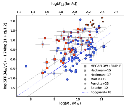
To better understand the evolutionary state of the various samples, we show the selected literature galaxy samples and MEGAFLOW+SIMPLE (Schroetter et al., 2015) galaxies relative to the main sequence between SFR and galaxy stellar mass in Fig. 1. In order to account for the redshift evolution, we choose to use the relation derived by Boogaard et al. (2018) and “normalized” for a redshift . In this figure, we clearly see that H15 galaxies are in the high SFR part, close to starburst galaxies, whereas MEGAFLOW and M19 galaxies appear to be mainly located on the main sequence at . In Fig. 1, red symbols represent either starbursts (for P23 and H17) or “strong” outflow cases (for H15, M19 and Paper III galaxies) as described in § 3.1.
3 Results
In order to compare wind studies using background quasars to other types of studies, we first need to establish a common framework. In particular, H15 makes a distinction between “strong” and “weak” outflows based on the wind momentum compared to the momentum injection rate from SFR and extend their formalism to winds probed by background quasars sight-lines.
3.1 Wind formalism
Following H15, in the case of momentum-driven winds where the momentum injection rate is supplied by the star-forming or starburst galaxy, the outward force from the momentum injection is countered by gravity. For an outflow to develop, the outward force ought to be greater than gravity, defining a critical momentum injection rate (e.g. H15).
For a cloud outflow model (to be consistent with Bouché et al. 2012 and Schroetter et al. 2015), the outward force is the pressure times the cloud area ,
| (1) |
where is the wind solid angle and the location of the wind, while the inward gravitational force is
| (2) |
where is the gravitational constant and the galaxy circular velocity. For a cloud of mass and area , the critical momentum flux is given by , or , such that, if one writes the cloud mass as where is the cloud column density and is the mean mass per particle, the critical momentum flux is
| (3) | |||||
This critical momentum flux required in order to have a net outward force on an outflowing cloud is [H15]:
| (4) |
In other words, winds will only develop when .
Comparing this critical momentum flux to the momentum injection rate , which is dynes, one can distinguish between “weak” and “strong” outflows. H15 defined “weak” winds when and “strong” winds when . This means that these regimes are the two cases where their momentum flux is larger or lower than ten times the critical momentum flux required to have a net outward force on an outflowing cloud. H15 made this arbitrary limit to where the “strong” outflow seems to carry a significant amount (of the order of unity) of the momentum flux available from the starburst.
From Eqs 1–2, the equation of motion for such a cloud launched from is (e.g. Murray et al., 2005; Heckman et al., 2015):
| (5) | |||||
| (6) |
where defines the radius at which the velocity peaks at
where (defined as in Heckman et al., 2015).
Note that this formalism makes a number of implicit assumptions. First, it assumes that the potential is that of an isothermal sphere, , which implies that is independent of radius. Second, the expression for the critical momentum injection rate is estimated at where is the launch radius. H15 uses =1 kpc.
In the case of background sight lines, the critical momentum is only evaluated at , where is the impact parameter. However, assuming that outflows are mass conserving, i.e. is constant, such that is conserved, then Eq.3 implies that is independent of radius, , provided that the circular velocity is roughly constant.
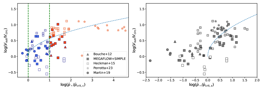
Following H15, we also looked at a shell model for the outflowing gas444The shell wind model assumes that the outward force is larger than the shell gravity for a shell mass at radius . using the critical momentum injection , where the shell mass fraction is . Fig. 2(right) shows that a shell model (Eq. 6 in H15) does not match the data compared to the cloud model shown in the left panel. We thus stick with the cloud model as it appears to better describe the data.
3.2 A universal formalism?
In order to test this formalism, we first compare the outflow velocity to the wind strengths in Figure 2. This figure shows the normalize outflow velocity as a function of ratio for the MEGAFLOW (paper III), H15, M19 555Note that for M19 systems, we only use those with a Mg ii REW larger than 0.5 Å in order to match the MEGAFLOW sample selection and have a consistent estimation of the hydrogen column density, which reduces the number of galaxies from 16 to 8 for this sample. and P23 galaxies for a cloud and a shell model on left and right panels, respectively. For the galaxies in paper III, we use where is the “intrinsic” galaxy rotational velocity (corrected for the galaxy inclination), while H15 used the observed rotational velocity. Finally, we use the bi-conical shape of our outflows with a cone opening angle of because of the azimuthal bi-modality in Mg ii (Bordoloi et al., 2011; Bouché et al., 2012; Schroetter et al., 2015; Lundgren et al., 2021). This leads to a downward correction of H15 estimations of their ejected mass rate 666 To get from a spherical to a bi-conical outflow with opening angles of 60 degrees geometry, the reduction is approximately 8.. We also use their updated outflow velocities values (Heckman & Borthakur, 2016). In addition, we investigated for a possible correlation between sight-line impact parameter and whether the outflow is classified as “strong” or “weak” but found none.
In Fig. 2 and subsequently, we use blue (red) symbols for “weak” (“strong”) outflows when showing MEGAFLOW, H15, M19 and P23 results. Also, throughout the paper, white squares correspond to galaxies in Paper III where the wind model does not fit the spectra convincingly777The reasons for each case are described in paper III, one of the main reason is that the absorption system has multiple component and thus is too complex to be reproduced by the simple wind model as the absorption most likely is a combination of multiple galaxy contribution.. In addition to differentiating “weak” and “strong” outflows in blue and red, respectively, we also use empty markers for “down-the-barrel” cases, namely H15 and P23, throughout the paper for a clear distinction between both methods.
3.3 Wind scaling relations
Because galaxy properties like SFR and mass are thought to be directly linked with properties of galactic winds (e.g. Heckman et al., 2000; Martin, 2005; Hopkins et al., 2012; Newman et al., 2012; Heckman et al., 2015) , we will investigate the relations, if any, between outflow properties like their velocity , their ejected mass rate and their loading factor with these main galaxy properties.
3.3.1 Scaling relations involving
To estimate , one does not necessarily need a background quasar. Indeed, many other studies derived outflow velocities with enough accuracy (; e.g Martin, 2005; Genzel et al., 2011; Newman et al., 2012; Arribas et al., 2014; Heckman et al., 2015). Those studies found a significant, but scattered, correlation between the outflow velocity and galaxy SFRs at low redshift (Heckman et al., 2000; Martin, 2005; Rupke et al., 2005; Martin et al., 2012; Arribas et al., 2014; Heckman et al., 2015). Martin (2005) derived an upper limit on as a function of SFR. This limit corresponds to the upper envelope of the outflow velocity distribution at a given SFR.
We show in Appendix A that down-the-barrel and background quasar derived outflow velocities give similar outflow speeds and are therefore comparable. Also, it is worth mentioning that background quasar measurements are made at larger radii than down-the-barrel and hence suffer from time travel effects that could obscure correlations with SFR if the SFR varies in time. This effect is discussed in papers II and III and is one of the reasons only galaxy-quasar pairs that have impact parameters kpc were selected in these studies. This reduces the possible effect of this time traveling effect on SFR estimation but does not remove it completely.
In Fig. 3, we investigate the dependence of on SFR, SFR surface density, , and , in the top left, middle and right panels, respectively. In the left panel, we corrected the SFRs for the redshift evolution of the MS using Boogaard et al. (2018) in order to have all SFRs at the same redshift ( in this case to match H15). The dashed black line represents the upper outflow velocity found by Martin (2005) for a small sample of local galaxies. They found that increases with SFR and their upper limit seems to under-estimate for a given SFR.
The red dot-dashed line in the top left and middle panels represents the positive correlation found by H15 and Heckman & Borthakur (2016). The red (blue) line with the shaded area represents our power law fit (which uses least squares fitting method) of the “strong” (“weak”) population, respectively, and its error obtained using the bootstrap method on 100k realizations. We find that the correlation between and the reduced SFR is positive for the “strong” outflows (). For the “weak” outflows in blue, a weaker correlation can be seen (). The bootstrap fitting results are given in Table 2.
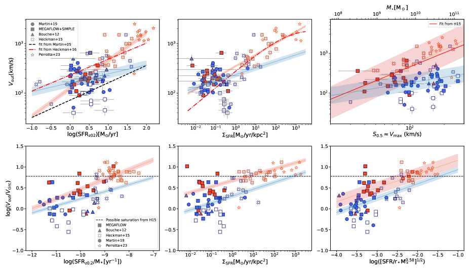
Concerning the correlation between and SFR surface density (), there have been disagreements about its existence (e.g. Chen et al., 2010; Rubin et al., 2014; Genzel et al., 2011; Newman et al., 2012). In the top middle panel of Figure 3, we shows the outflow velocity as a function of 888Since is correlated by the galaxy size which is correlated with , we thus do not normalize for redshift evolution for this quantity.. Heckman & Borthakur (2016) found a strong correlation between those two quantities. Adding our observations as well as M19 to their sample confirms this correlation.
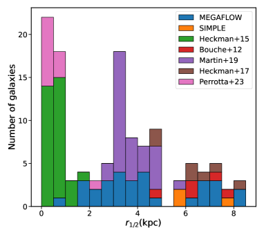
We also point out that the H15 are large compared to those of MEGAFLOW galaxies. Looking at Figure 1, H15 galaxies having larger SFRs than MEGAFLOW ones. To check whether the large of H15 were due to only SFRs or also sizes, Figure 4 shows the distribution of half-light radius of samples used in this study. We see that H15 galaxies tend to be a much smaller. This contributes to the fact that their are quite large compared to MEGAFLOW or M19 galaxies. Using the same bootstrap method as for the first top left panel of this figure, there is no large difference between “strong” and “weak” outflows, and , respectively.
The next step is to investigate whether the outflow velocity depends on the host galaxy mass. Following the SFR- relation (Fig. 1) and the tendency of to increase with the host galaxy star formation rate, we could expect the outflow velocity to correlate also with the host galaxy mass. However, a more massive galaxy has a deeper gravitational well, and thus it is more difficult for gas to accelerate. The top right panel of Figure 3 shows the relation between and . For the “weak” outflows from MEGAFLOW and M19 shown in blue, outflow velocities are almost constant at around 100-200 km s-1 , while for “strong” outflows (red points) indeed strongly correlates with galaxy mass, which confirms the results from H15, represented by the red curve on this top right panel. Using the bootstrap fitting method, we indeed find that “strong” outflows have a larger slope with () than in the case for “weak” outflows ().
To summarize, correlates with SFR as well as with . also correlates with the host galaxy mass if outflows are “strong” and is weakly mass-dependent for “weak” outflows. In other words, we begin to see a difference in outflow properties between “weak” and “strong” outflows where “strong” outflows appears to correlate more strongly with galaxy properties than “weak” ones. Distinguishing between those two outflow populations allows us to confirm that the formalism of H15 is relevant to SFGs and starbursts.
In order to investigate further the possible scaling relations for the outflow velocity, we show, in the bottom row of Figure 3, normalized by the galaxy circular velocity as a function of specific SFR corrected to (bottom left panel), SFR surface density () (bottom middle panel) and a combination of specific SFR and (bottom right panel).
One sees that the relative outflow speed is a simple function (universal?) of SFR, or momentum injection rate (bottom left), and that, as mentioned in H15, there is a possible saturation in normalized outflow velocity when above . This saturation is shown with the horizontal black dashed line in each panel of the bottom row of Fig 3. We can see that this saturation looks to be the case if we only look at H15 data. However, with the addition of the lower SFR data (MEGAFLOW + M19), that is no longer as convincing. In these bottom panels we also show the bootstrap fits for each outflow population in red and blue lines for “strong” and “weak”, respectively. Apart from the normalization of each fit, “strong” and “weak” outflows appear to correlate similarly with each quantity. Those correlations are less scattered than with SFR, or with which we can directly compare with the top row and there is no clear differentiation between both outflow populations if we consider them together or independently (as shown by the corresponding correlation coefficients in Table 2).
3.3.2 Scaling relations for
We now turn to another fundamental wind property, namely the ejected mass outflow rate (and the mass loading factor SFR) and investigate possible scaling relations with the properties of the host galaxies.
In order to compare the outflow ejection rates of paper III to H15 who estimated the mass ejection rate assuming spherically symmetric outflows with sr , we scaled their to 60∘ using, as previously, from Heckman & Borthakur (2016).
Concerning M19 galaxies, to estimate the mass ejection rate we used the Mg ii REW as a proxy to estimate the column density (Ménard & Chelouche, 2009; Zhu & Ménard, 2013). This proxy is only viable for strong Mg ii REW and we thus only select the galaxies with .
Similar to Figure 3, the top panels of Figure 5 shows the mass ejection rate () as a function of SFR corrected to (left panel), (middle panel) and the galaxy mass (right panel). Regarding the -SFR relation, Hopkins et al. (2012) predicted that (shown as the dashed red line in the left panel) whereas Arribas et al. (2014) observed a steeper index (shown as a solid black line).
The amount of ejected mass by supernova explosions being directly linked to SFR, it is intuitively expected that SFR correlates with . Looking by eye only at “weak” outflows in blue, there is no obvious correlation, but for “strong” outflows (in red) the correlation between the mass ejection rate and the galaxy SFR appears to be more in agreement with Hopkins et al. (2012)’s predictions than with the observations of Arribas et al. (2014). As for , we use the bootstrap fitting method to measure the relations between and the galaxy properties. Looking at the top left panel of Figure 5, both “strong” and “weak” outflows correlate slightly with SFR and bootstrap slopes are close to each other, with the “strong” outflows having a steeper slope than the “weak”, and for both “strong” and “weak” populations, respectively.
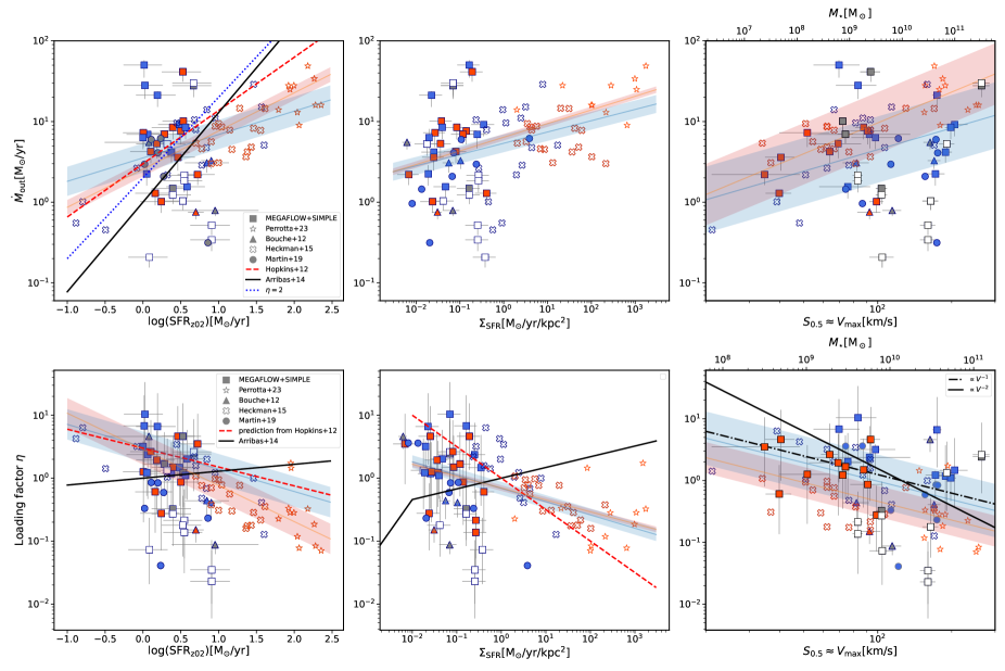
Contrary to the correlation between and , the top middle panel of Fig. 5 shows that there is no correlation between the mass outflow rate and , except perhaps a mild relation, which is confirmed by the bootstrap fitting as for “strong” and for “weak” outflows. Similarly, the top right panel of Fig. 5 indicates a weak correlation between the ejected mass rate and (and thus its stellar mass) for both “strong” and “weak” outflows, albeit also with a large scatter ( for the “weak” populations and for the “strong” ones).
3.3.3 Scaling relations for
The last but maybe the most important parameter concerning galactic outflows is the mass loading factor , i.e. the ratio between the mass ejection rate and the SFR of the galaxy;
| (8) |
if
Depending on the value of in Equation 8, we can differentiate 3 cases: the correlation between and SFR is either positive (), negative () or can be constant (). Those three possibilities are represented by the lines in top left panel of Figure 5 with (Hopkins et al., 2012), (Arribas et al., 2014) and (a constant loading factor ), none of which actually fit the data. If a correlation exists, it has a lower than Hopkins et al. (2012). Indeed, according to the result of the bootstrap method in Table 2, is around 0.4 regardless of outflow strength. Thus, we can argue that if correlates with SFR, it should be an anti-correlation (). The bottom left panel of Figure 5 shows the mass loading factor as a function of SFR. We can see a scattered anti-correlation between these two properties. This confirms that with . Our observations are thus in qualitative agreement with Hopkins et al. (2012) predictions.
As there is no significant difference between “weak” and “strong” outflows we can conclude that the mass loading factor indeed anti-correlates with the galaxy SFR regardless of the galaxy type. Thus, galaxies with high SFR tend to have a lower mass loading factor than galaxies with a lower SFR. We will return to the implications of this result in § 4.
As before, we would like to investigate whether the mass loading factor depends on local galaxy properties (such as ) or global (such as mass). In the bottom middle panel of Figure 5, we show as a function of . Prediction and observations from Hopkins et al. (2012) and Arribas et al. (2014) are represented by red-dashed and black lines respectively. It appears that there is a clear anti-correlation between and in the data. The slope of this anti-correlation seems to be the same for “strong” and “weak” outflows and the bootstrap fitting gives us the same slope for both populations (-0.2).
It is worth mentioning that Arribas et al. (2014) and Newman et al. (2012) found that galaxies (low- galaxies from Arribas et al. (2014) and high- galaxies from Newman et al. (2012)) require a larger than 1 M⊙ yr-1 kpc-2 for launching strong outflows. This statement is not supported by either MEGAFLOW or M19 galaxies since the majority of them show outflow signatures and have below 1 M⊙ yr-1 kpc-2, even if we only focus on “strong” outflows shown in red.
As seen in bottom right panel of Figure 5, the mass loading factor anti-correlates with the galaxy stellar mass. Concerning the correlation slopes, we will discuss their implication in the next section.
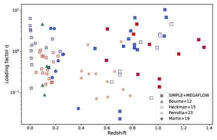
Another aspect about the mass loading factor is its redshift dependence. Indeed, as there is a peak in star-formation density at redshift 2-3 (e.g. Lilly et al., 1996; Madau et al., 1996; Behroozi et al., 2013), if correlates with SFR, one can expect a correlation between and redshift. We thus investigated this relation but found no evident correlation (as compared to Muratov et al., 2015). Figure 8 in the appendix shows as a function of redshift for individual cases of each study and shows no apparent correlation. Finally, we find no correlation between and , in agreement with results from H15.
4 What mechanisms drive galactic winds?
We will now use the results shown in the previous section to tackle the question what mechanisms drive galactic winds out of the galactic disk. To date, there are two major mechanisms which could be responsible for driving materials out of the galaxy: energy-driven and momentum-driven outflows (as reviewed in Heckman et al., 2017). The momentum-driven wind scenario considers that the two primary sources of momentum deposition in driving galactic winds are supernovae and radiation pressure from the central starburst. This model assumes that is constant and implies that must be inversely proportional to , i.e. , given that scales as and thus as the galaxy circular velocity (e.g. Martin, 2005; Oppenheimer & Davé, 2006, 2008; Davé et al., 2011; Heckman et al., 2017).
Energy-driven wind model assumes that when stars evolve, they deposit energy into the ISM. The amount of gas blown out of the disk is assumed to be proportional to the total energy released by supernovae and inversely proportional to the escape velocity squared. In the energy-driven scenario, energy conservation implies (e.g. van den Bosch, 2002).
In the bottom right panel of Figure 5, we show the mass loading factor as a function of galaxy 999We choose to use as we used this parameter to derive galaxy stellar masses. It is more appropriate to use this factor than the maximum rotation velocity as some of our galaxies are dispersion-dominated. (bottom x-axis) and galaxy stellar mass (top x-axis). In addition, we also show (the black line in the bottom right panel) in order to see if we could discriminate between the two mechanisms for driving outflows.
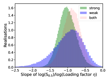
If we do not distinguish between “weak” and “strong” outflows, we find a scatter anti-correlation between and with a slope of . This slope value does not allow us to differentiate between momentum and energy-driven scenarios but points toward a momentum-driven scenario nonetheless. Looking at “strong” and “weak” outflow populations individually, we find that the anti-correlation with the galaxy stellar mass is steeper. Applying the bootstrap method to create 100k realisations of the “weak” and “strong” groups with 39 and 43 data points respectively, as well as for the combined data, the resulting histogram of the fitted slopes of the loading factor – relation is shown in Figure 6. We can see that using all the data points, the mass loading factor whereas for each population independently, we find and for “weak” and “strong” outflows, respectively.
This slope is consistent with the prediction of Hopkins et al. (2012) () and favors a momentum-driven scenario for galactic outflows.
5 Summary and Conclusions
In this paper, we used the results published in Paper III on outflow properties inferred from quasar absorption lines and compared them with other studies reporting mass ejection rates in order to investigate possible scaling relations between outflows and their host galaxy properties. The three main parameters we investigated are the outflow velocity , the mass ejection rate and the mass loading factor . Those parameters were related to global galaxy properties like SFR, stellar mass and SFR surface density.
We distinguished between two outflow regimes: “weak” and “strong” outflows (see § 2.2). These regimes are the two cases where their momentum flux is larger or lower than ten times the critical momentum flux required to have a net outward force on an outflowing cloud, i.e. “weak” if and “strong” if . For each parameter combination, we used a bootstrap method in order to estimate the power law slopes of the relations between the aforementioned properties. The two regimes show different behaviours as can be summarize as follows:
| Parameters | “strong” | “weak” | Both |
|---|---|---|---|
| (1) | (2) | (3) | (4) |
| 0.560.05 | 0.180.09 | 0.460.05 | |
| 0.230.03 | 0.130.05 | 0.230.02 | |
| 1.330.20 | 0.450.21 | 0.770.18 | |
| 0.470.09 | 0.290.17 | 0.400.08 | |
| 0.160.04 | 0.130.11 | 0.170.04 | |
| 1.270.21 | 0.890.41 | 1.090.21 | |
| -0.570.24 | -0.350.24 | -0.430.13 | |
| -0.180.04 | -0.210.10 | -0.190.04 | |
| -1.010.24 | -0.990.43 | -0.890.25 |
(1) Wind parameters: outflow velocity , ejected mass rate and the mass loading factor as a function of (if any correlation) , and ; (2) “strong” outflow population; (3) “weak” outflow population; (4) Both populations altogether.
The outflow velocity correlates with SFR, and and shows stronger correlations for the “strong” outflow population. In particular, exceeds the upper limit of Martin (2005) concerning its correlation with SFR.
The mass ejection rate correlates, as the outflow velocity, with the three galaxy properties for both populations but the “strong” outflows does not clearly correlate with SFR surface density.
Finally, the mass loading factor anti-correlates with SFR, and for both populations. However, is apparently not redshift dependent. Details on the different slopes are summarized in Table 2.
We also find that the galaxy does not need M⊙ yr-1 kpc-2 in order to be able to launch material out of the galactic disk.
In addition, we addressed the question which mechanism is dominant andor responsible for launching outflows. According to the bottom right panel of Figure 5, we find that both “weak” and “strong” outflows point towards a momentum-driven scenario as the coefficient found for both populations is close to with and . This result needs to be confirmed with additional and more accurate results but it shows that depending on the outflow “strength”, the mechanism responsible for launching the gas tends to be the same for the “strong” and “weak” outflow regimes.
In conclusion, using a bootstrap method on all galaxies and for the two regimes individually, we saw that one needs to differentiate between “strong” and “weak” outflows as both regimes have different behaviors. This differentiation is thus important to understand the role of galactic outflows in galaxy formation and evolution. We compared outflow properties derived from quasar absorption line and down the barrel methods and showed that a universal formalism can be used for outflows regardless of the method used. We mentioned that the background quasar line method has larger impact parameter than down the barrel and can suffer from time travel effects that could obscure correlation with SFR if the SFR varies during the time needed for the gas to get from the galaxy to the quasar line of sight. As this effect is discussed in previous papers (papers I and III), we do not develop this effect here but are aware that this may have an effect on results implying SFRs. Some results on properties like mass loading factors or mass ejection rates have order of magnitudes uncertainties and are more indicative than accurate but allowed us to nonetheless draw some conclusions using a bootstrap fitting method. Using the MEGAFLOW results on outflow properties and differentiating between “weak” and “strong” outflows, we confirm scaling relations as well as open new paths in the understanding of galactic winds properties and thus the evolution and formation of galaxies. Accuracy is essential in order to get a correct answer for those scaling relations, especially concerning wind properties like the mass outflow rate and mass loading factor. The background source method would greatly benefit from an accurate estimation of the hydrogen column density to be able to estimate lower column densities that can be inferred from Mg ii absorption. Therefore, future observations are still needed. The James Webb Space Telescope allows for higher redshift outflow studies and will provide many more outflow cases.
Acknowledgments
We thank the referee for her/his helpful comments and suggestions which helped to greatly improve the paper. This work has been carried out thanks to the support of the Agence Nationale de la Recherche (ANR) grant 3DGasFlows (ANR-17-CE31-0017) as well as support from the Centre National d’Etudes Spatiales (CNES) through the APR program.
References
- Alam et al. (2015) Alam, S., Albareti, F. D., Allende Prieto, C., et al. 2015, ArXiv e-prints [arXiv:1501.00963]
- Alexandroff et al. (2015) Alexandroff, R. M., Heckman, T. M., Borthakur, S., Overzier, R., & Leitherer, C. 2015, The Astrophysical Journal, 810, 104
- Arribas et al. (2014) Arribas, S., Colina, L., Bellocchi, E., Maiolino, R., & Villar-Martín, M. 2014, A&A, 568, A14
- Bacon et al. (2010) Bacon, R., Accardo, M., Adjali, L., et al. 2010, in Society of Photo-Optical Instrumentation Engineers (SPIE) Conference Series, Vol. 7735, Society of Photo-Optical Instrumentation Engineers (SPIE) Conference Series, 8
- Bacon et al. (2006) Bacon, R., Bauer, S., Böhm, P., et al. 2006, Msngr, 124, 5
- Bacon et al. (2015) Bacon, R., Brinchmann, J., Richard, J., et al. 2015, A&A, 575, A75
- Behroozi et al. (2013) Behroozi, P. S., Wechsler, R. H., & Conroy, C. 2013, ApJ, 762, L31
- Bergeron & Stasinska (1986) Bergeron, J. & Stasinska, G. 1986, A&A, 169, 1
- Boogaard et al. (2018) Boogaard, L. A., Brinchmann, J., Bouché, N., et al. 2018, A&A, 619, A27
- Bordoloi et al. (2011) Bordoloi, R., Lilly, S. J., Knobel, C., et al. 2011, ApJ, 743, 10
- Bouché et al. (2012) Bouché, N., Hohensee, W., Vargas, R., et al. 2012, MNRAS, 426, 801
- Bouché et al. (2007) Bouché, N., Murphy, M. T., Péroux, C., et al. 2007, ApJ, 669, L5
- Chabrier (2003) Chabrier, G. 2003, PASP, 115, 763
- Chen et al. (2020) Chen, H.-W., Zahedy, F. S., Boettcher, E., et al. 2020, MNRAS, 497, 498
- Chen et al. (2010) Chen, Y., Tremonti, C. A., Heckman, T. M., et al. 2010, AJ, 140, 445
- Davé et al. (2011) Davé, R., Finlator, K., & Oppenheimer, B. D. 2011, ArXiv e-prints
- Dekel & Silk (1986) Dekel, A. & Silk, J. 1986, ApJ, 303, 39
- Dekker et al. (2000) Dekker, H., D’Odorico, S., Kaufer, A., Delabre, B., & Kotzlowski, H. 2000, in Proc. SPIE, Vol. 4008, Optical and IR Telescope Instrumentation and Detectors, ed. M. Iye & A. F. Moorwood, 534–545
- Genzel et al. (2011) Genzel, R., Newman, S., Jones, T., et al. 2011, ApJ, 733, 101
- Grimes et al. (2009) Grimes, J. P., Heckman, T., Aloisi, A., et al. 2009, ApJS, 181, 272
- Heckman et al. (2017) Heckman, T., Borthakur, S., Wild, V., Schiminovich, D., & Bordoloi, R. 2017, The Astrophysical Journal, 846, 151
- Heckman et al. (2015) Heckman, T. M., Alexandroff, R. M., Borthakur, S., Overzier, R., & Leitherer, C. 2015, ApJ, 809, 147
- Heckman & Borthakur (2016) Heckman, T. M. & Borthakur, S. 2016, The Astrophysical Journal, 822, 1
- Heckman et al. (2000) Heckman, T. M., Lehnert, M. D., Strickland, D. K., & Armus, L. 2000, ApJS, 129, 493
- Ho et al. (2017) Ho, S. H., Martin, C. L., Kacprzak, G. G., & Churchill, C. W. 2017, ApJ, 835, 267
- Hopkins et al. (2012) Hopkins, P. F., Quataert, E., & Murray, N. 2012, MNRAS, 421, 3522
- Kacprzak et al. (2011) Kacprzak, G. G., Churchill, C. W., Evans, J. L., Murphy, M. T., & Steidel, C. C. 2011, MNRAS, 416, 3118
- Kacprzak et al. (2014) Kacprzak, G. G., Martin, C. L., Bouché, N., et al. 2014, ApJ, 792, L12
- Lan & Fukugita (2017) Lan, T.-W. & Fukugita, M. 2017, ApJ, 850, 156
- Lilly et al. (1996) Lilly, S. J., Le Fevre, O., Hammer, F., & Crampton, D. 1996, ApJ, 460, L1
- Lofthouse et al. (2020) Lofthouse, E. K., Fumagalli, M., Fossati, M., et al. 2020, MNRAS, 491, 2057
- Lundgren et al. (2021) Lundgren, B. F., Creech, S., Brammer, G., et al. 2021, ApJ, 913, 50
- Madau et al. (1996) Madau, P., Ferguson, H. C., Dickinson, M. E., et al. 1996, MNRAS, 283, 1388
- Martin (2005) Martin, C. L. 2005, ApJ, 621, 227
- Martin et al. (2019) Martin, C. L., Ho, S. H., Kacprzak, G. G., & Churchill, C. W. 2019, ApJ, 878, 84
- Martin et al. (2012) Martin, C. L., Shapley, A. E., Coil, A. L., et al. 2012, ApJ, 760, 127
- Mary et al. (2020) Mary, D., Bacon, R., Conseil, S., Piqueras, L., & Schutz, A. 2020, A&A, 635, A194
- Ménard & Chelouche (2009) Ménard, B. & Chelouche, D. 2009, MNRAS, 393, 808
- Moster et al. (2013) Moster, B. P., Naab, T., & White, S. D. M. 2013, MNRAS, 428, 3121
- Muratov et al. (2015) Muratov, A. L., Kereš, D., Faucher-Giguère, C.-A., et al. 2015, MNRAS, 454, 2691
- Murray et al. (2005) Murray, N., Quataert, E., & Thompson, T. A. 2005, ApJ, 618, 569
- Muzahid et al. (2015) Muzahid, S., Kacprzak, G. G., Churchill, C. W., et al. 2015, ApJ, 811, 132
- Muzahid et al. (2020) Muzahid, S., Schaye, J., Marino, R. A., et al. 2020, MNRAS, 496, 1013
- Newman et al. (2012) Newman, S. F., Shapiro Griffin, K., Genzel, R., et al. 2012, ApJ, 752, 111
- Nielsen et al. (2013) Nielsen, N. M., Churchill, C. W., Kacprzak, G. G., & Murphy, M. T. 2013, ApJ, 776, 114
- Nielsen et al. (2015) Nielsen, N. M., Churchill, C. W., Kacprzak, G. G., Murphy, M. T., & Evans, J. L. 2015, ApJ, 812, 83
- Oppenheimer & Davé (2006) Oppenheimer, B. D. & Davé, R. 2006, MNRAS, 373, 1265
- Oppenheimer & Davé (2008) Oppenheimer, B. D. & Davé, R. 2008, MNRAS, 387, 577
- Perrotta et al. (2023) Perrotta, S., Coil, A. L., Rupke, D. S. N., et al. 2023, ApJ, 949, 9
- Rahmani et al. (2018) Rahmani, H., Péroux, C., Schroetter, I., et al. 2018, MNRAS, 480, 5046
- Ross et al. (2012) Ross, N. P., Myers, A. D., Sheldon, E. S., et al. 2012, ApJS, 199, 3
- Rubin et al. (2014) Rubin, K. H. R., Prochaska, J. X., Koo, D. C., et al. 2014, ApJ, 794, 156
- Rupke et al. (2005) Rupke, D. S., Veilleux, S., & Sanders, D. B. 2005, ApJS, 160, 115
- Schroetter et al. (2015) Schroetter, I., Bouché, N., Péroux, C., et al. 2015, ApJ, 804, 83
- Schroetter et al. (2016) Schroetter, I., Bouché, N., Wendt, M., et al. 2016, ApJ, 833, 39
- Schroetter et al. (2019) Schroetter, I., Bouché, N. F., Zabl, J., et al. 2019, MNRAS, 2451
- Silk & Rees (1998) Silk, J. & Rees, M. J. 1998, A&A, 331, L1
- Steidel et al. (1995) Steidel, C. C., Bowen, D. V., Blades, J. C., & Dickinson, M. 1995, ApJ, 440, L45
- Steidel et al. (2014) Steidel, C. C., Rudie, G. C., Strom, A. L., et al. 2014, ApJ, 795, 165
- Turner et al. (2014) Turner, M. L., Schaye, J., Steidel, C. C., Rudie, G. C., & Strom, A. L. 2014, MNRAS, 445, 794
- van den Bosch (2002) van den Bosch, F. C. 2002, MNRAS, 331, 98
- Zabl et al. (2019) Zabl, J., Bouché, N. F., Schroetter, I., et al. 2019, MNRAS, 485, 1961
- Zhu & Ménard (2013) Zhu, G. & Ménard, B. 2013, ApJ, 770, 130
Appendix
On measuring outflows speeds
To estimate the outflow velocity, there are differences between background quasar and galaxy absorption (aka “down the barrel”) methods. The main difference is the background object. For quasar sightlines, it is known that the probed gas is likely to be in the CGM while for galaxies (down the barrel), the gas can be anywhere in the CGM or IGM towards the observer. A background quasar also gives the location of the absorbing gas, namely the impact parameter, whereas absorption in a galaxy spectrum does not provide such information and is usually assumed to be several kpc from the host galaxy.
In addition to this difference, the outflow absorption profile is different. In H15, the observer looks directly at the galaxy. The outflowing gas ejected from this galaxy is moving toward the observer. Thus, this gas gives rise to blue-shifted absorption in the galaxy spectrum. In order to see this blue-shifted absorption, the host galaxy needs to have a low inclination (to be close to a face-on configuration). Using a background quasar, the outflow absorption can be either blue or red-shifted with respect to the host galaxy systemic redshift. In addition, host galaxies are selected to be not face-on. As a matter of fact, host galaxies selected in paper III needed to have an inclination for low position angle uncertainties.
To assess those differences and thus confirm that we obtain similar results on the outflow velocity using our wind model, we first need to create a configuration similar to the H15 method, namely a down-the-barrel configuration. We then create a wind model for this specific geometry. For a face-on galaxy, H15 use the outflow velocity value corresponding to of the blue-shifted absorption produced by the outflowing gas. This value will give the outflow velocity ,90. This ,90 is then corrected in Heckman & Borthakur (2016) to have the maximum outflow velocity of the gas. This maximum outflow velocity corresponds to our definition of . We thus try to see if the derived by H15 is similar to the one we derive from our wind model.
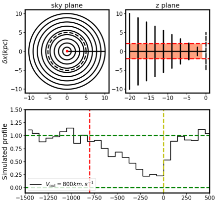
The aim is to see if we can reproduce the blue-shifted absorption shape of their data seen in Figure 1 of their paper and also where ends up. We create a wind model of a galaxy with an inclination of , azimuthal angle of 90∘ and an impact parameter of 0 kpc.
This model is shown in Figure 7. The top left panel of this Figure is a representation of the sky plane of the face-on galaxy with the outflowing cone directed towards the observer. The top right panel represents a side view of the system, showing the line of sight (LOS) in orange crossing the outflowing cone from right to left. Since the LOS crosses all the way from the galaxy to the outer part of the cone, we create an accelerated wind model (as we are tracing the accelerating part of the outflow, this model is described in Schroetter et al. 2015)). This accelerated wind model changes the asymmetry of the profile as there are more clouds with lower velocity close to the galaxy.
The bottom panel of Figure 7 shows the resulting absorption profile of this configuration. The red vertical dashed line represents the input . We see that this outflowing velocity corresponds to the furthest part of the blue-shifted absorption. This is in agreement with the derived by H15, corrected in Heckman & Borthakur (2016). We can thus directly compare our results with those of H15.
Even if we do not include galaxies from Arribas et al. (2014) we will still consider the relations they found to see if there are significant differences between SFGs and Ultra/Luminous infrared galaxies outflow properties.
Concerning M19 galaxies, they use the background quasars method and thus we can easily derive their outflow velocities. For their galaxies, we use the maximum velocity offsets (blue or red-shifted) of the Mg ii absorptions seen in background quasars as projected outflow velocities. Then, using the inclination derived in their study and a cone opening angle of 30∘, we get the estimated outflow velocities . From those outflow velocities, impact parameters and , we estimate the mass outflow rates using equation 5 of Schroetter et al. (2015). Then, mass loading factors are estimated using SFRs. Since their SFRs are derived using M19 main sequence figure, we emphasize that those results are more indicative than accurate.
For P23 outflow velocities, like M19, we assume the outflow velocity to be the maximum Mg ii absorption velocity offsets. We note that they also have Fe ii absorption velocities but for consistency we choose to only use the Mg ii ones since we do the same for background quasars. P23 also already have ejected mass outflow rate for bi-conical outflow geometry as well as corresponding loading factors, we thus do not need to re-estimate them.
Mass loading factor redshift evolution
Figure 8 shows the mass loading factor as a function of host galaxy redshift. As mentioned in the text, there is no apparent correlation between the mass loading factor and the host galaxy redshift.
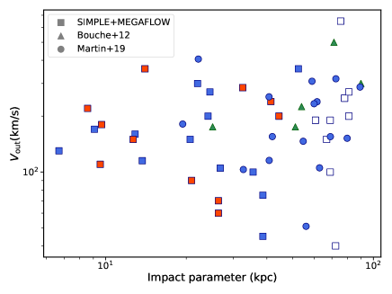
Outflow velocity versus impact parameter
Figure 9 shows the outflow velocity as a function of impact parameter for background source studies. As mentioned in the text, there is no apparent correlation between those parameters.
Galaxy properties
The following tables list all the galaxy properties used in this paper in order to be able to reproduce the results.
| Study | Vout | ||||||||
|---|---|---|---|---|---|---|---|---|---|
| (1) | (2) | (3) | (4) | (5) | (6) | (7) | (8) | (9) | (10) |
| Paper III | 180.0 | 0.461 | 0.0253 | 40.38 | 1.799 | 4.984 | 33.53 | 32.35 | 32.60 |
| 360.0 | 0.025 | 0.0698 | 83.16 | 14.04 | 10.39 | 34.11 | 33.75 | 33.85 | |
| 200.0 | 0.376 | 0.0254 | 188.6 | 2.085 | 1.179 | 34.22 | 33.84 | 35.27 | |
| 100.0 | 0.320 | 0.0177 | 190.8 | 2.642 | 1.334 | 34.27 | 34.22 | 35.29 | |
| 150.0 | 0.482 | 0.3487 | 205.5 | 4.593 | 1.470 | 34.47 | 34.16 | 35.42 | |
| 170.0 | 0.062 | 0.2500 | 92.67 | 3.464 | 2.367 | 34.14 | 33.26 | 34.04 | |
| 70.0 | 0.546 | 0.2656 | 82.87 | 1.079 | 0.249 | 34.61 | 32.93 | 33.84 | |
| 650.0 | 0.527 | 0.1906 | 93.61 | 20.69 | 4.620 | 34.63 | 33.50 | 34.06 | |
| 160.0 | 0.583 | 0.0470 | 75.55 | 0.776 | 3.025 | 33.39 | 32.58 | 33.68 | |
| 90.0 | 0.242 | 0.0237 | 98.98 | 0.509 | 0.275 | 34.24 | 32.85 | 34.15 | |
| 250.0 | 0.533 | 0.0379 | 72.09 | 5.061 | 1.226 | 34.59 | 33.14 | 33.60 | |
| 100.0 | 0.394 | 0.1627 | 103.6 | 0.617 | 0.270 | 34.33 | 33.85 | 34.23 | |
| 45.0 | 0.908 | 0.2547 | 160.0 | 0.170 | 0.022 | 34.85 | 33.98 | 34.99 | |
| 240.0 | 0.394 | 0.0848 | 87.68 | 4.236 | 1.489 | 34.43 | 33.37 | 33.94 | |
| 270.0 | 0.191 | 0.0225 | 174.0 | 10.60 | 6.615 | 34.18 | 34.19 | 35.13 | |
| 40.0 | 0.086 | 0.3769 | 104.3 | 0.103 | 0.073 | 34.13 | 33.60 | 34.24 | |
| 220.0 | 0.005 | 0.0270 | 51.75 | 3.632 | 2.268 | 34.18 | 32.60 | 33.03 | |
| 270.0 | 0.667 | 0.0698 | 264.1 | 15.04 | 2.623 | 34.74 | 34.80 | 35.86 | |
| 300.0 | 0.016 | 0.1635 | 69.61 | 25.11 | 20.32 | 34.07 | 33.62 | 33.54 | |
| 200.0 | 0.500 | 0.1397 | 91.09 | 3.819 | 0.866 | 34.62 | 33.53 | 34.01 | |
| 150.0 | 0.527 | 0.0413 | 164.1 | 0.517 | 0.178 | 34.44 | 34.07 | 35.03 | |
| 360.0 | 0.722 | 0.0068 | 34.69 | 1.100 | 7.013 | 33.17 | 31.78 | 32.33 | |
| 150.0 | 0.103 | 0.0808 | 63.81 | 2.124 | 2.640 | 33.88 | 32.71 | 33.39 | |
| 110.0 | 0.161 | 0.4056 | 39.78 | 0.645 | 1.138 | 33.73 | 32.01 | 32.57 | |
| 190.0 | 0.286 | 0.1179 | 73.94 | 3.485 | 1.673 | 34.30 | 33.03 | 33.65 | |
| 285.0 | 0.183 | 0.0360 | 69.06 | 2.660 | 2.582 | 33.99 | 32.96 | 33.53 | |
| 190.0 | 0.394 | 0.1627 | 103.6 | 0.742 | 0.325 | 34.33 | 33.85 | 34.23 | |
| 75.0 | 0.908 | 0.2547 | 160.0 | 0.259 | 0.034 | 34.85 | 33.98 | 34.99 | |
| 200.0 | 0.667 | 0.0698 | 264.1 | 13.92 | 2.429 | 34.74 | 34.80 | 35.86 | |
| 60.0 | 0.546 | 0.2656 | 82.87 | 0.925 | 0.214 | 34.61 | 32.93 | 33.84 | |
| H15 | 350 | 15.0 | 8.5113 | 83 | 33.0 | 0.300 | 34.9 | 33.4 | 33.9 |
| 530 | 24.0 | 36.307 | 108 | 26.0 | 0.175 | 35.1 | 33.4 | 34.3 | |
| 450 | 37.0 | 3.1622 | 161 | 97.0 | 0.409 | 35.3 | 34.4 | 35.0 | |
| 1500 | 19.0 | 19.952 | 184 | 39.0 | 0.769 | 35.0 | 33.9 | 35.3 | |
| 1500 | 8.0 | 213.79 | 115 | 9.0 | 0.376 | 34.6 | 32.8 | 34.4 | |
| 370 | 10.0 | 13.182 | 52 | 34.0 | 0.308 | 34.7 | 32.8 | 33.1 | |
| 1500 | 29.0 | 7.7624 | 225 | 74.0 | 0.996 | 35.2 | 34.4 | 35.6 | |
| 550 | 10.0 | 3.4673 | 72 | 48.0 | 0.942 | 34.7 | 33.4 | 33.6 | |
| 520 | 11.0 | 3.9810 | 88 | 37.0 | 0.780 | 34.7 | 33.5 | 34.0 | |
| 360 | 8.0 | 3.2359 | 77 | 30.0 | 0.703 | 34.6 | 33.4 | 33.7 | |
| 990 | 29.0 | 41.686 | 151 | 30.0 | 0.284 | 35.1 | 33.7 | 34.9 | |
| 510 | 7.0 | 0.9549 | 94 | 99.0 | 2.003 | 34.5 | 33.8 | 34.1 | |
| 570 | 9.0 | 2.4547 | 123 | 45.0 | 1.228 | 34.6 | 33.9 | 34.6 | |
| 370 | 5.0 | 2.0417 | 48 | 3.5 | 1.079 | 34.4 | 33.0 | 32.9 | |
| 780 | 23.0 | 102.32 | 132 | 15.0 | 0.158 | 35.0 | 33.3 | 34.7 | |
| 440 | 14.0 | 4.3651 | 94 | 47.0 | 0.559 | 34.8 | 33.6 | 34.1 | |
| 660 | 27.0 | 51.286 | 88 | 21.0 | 0.178 | 35.1 | 33.2 | 34.7 | |
| 490 | 6.0 | 6.9183 | 94 | 21.0 | 0.765 | 34.5 | 33.3 | 34.1 | |
| 700 | 9.0 | 5.6234 | 88 | 35.0 | 0.972 | 34.6 | 33.4 | 34.0 | |
| 1000 | 36.0 | 60.255 | 132 | 28.0 | 0.216 | 35.2 | 33.5 | 34.7 | |
| 1260 | 41.0 | 30.902 | 240 | 46.0 | 0.353 | 35.3 | 34.2 | 35.7 | |
| 150 | 0.83 | 0.2691 | 88 | 4.8 | 3.189 | 33.6 | 33.5 | 34.0 | |
| 60 | 0.32 | 0.5623 | 30 | 2.3 | 1.418 | 33.2 | 32.2 | 32.1 | |
| 230 | 5.0 | 0.4073 | 132 | 33.0 | 1.581 | 34.4 | 34.2 | 34.7 |
(1) Study, (2) outflow velocity (km s-1); (3) (M⊙ yr-1); (4) (M⊙ yr-1 kpc-2) ; (5) Galaxy maximum rotational velocity (or S0.5) (km s-1); (6) ejected mass rate (M⊙ yr-1); (7) Mass loading factor ; (8) Momentum injection rate; (9) Critical momentum flux; (10) Critical momentum flux for a shell model.
| Study | Vout | ||||||||
|---|---|---|---|---|---|---|---|---|---|
| (1) | (2) | (3) | (4) | (5) | (6) | (7) | (8) | (9) | (10) |
| H15 | 170 | 0.16 | 0.4466 | 55 | 1.0 | 6.324 | 32.9 | 32.7 | 33.2 |
| 190 | 6.0 | 2.6302 | 108 | 4.6 | 0.479 | 34.5 | 33.6 | 34.3 | |
| 630 | 2.8 | 1.1220 | 115 | 22.0 | 3.437 | 34.1 | 33.7 | 34.4 | |
| 340 | 40.0 | 16.982 | 240 | 12.0 | 0.127 | 35.3 | 34.3 | 35.7 | |
| 150 | 0.13 | 0.9120 | 68 | 1.0 | 4.242 | 32.8 | 32.6 | 33.5 | |
| 210 | 2.1 | 1.9498 | 72 | 5.4 | 1.038 | 34.0 | 33.1 | 33.6 | |
| 230 | 4.8 | 0.2344 | 132 | 30.0 | 2.191 | 34.4 | 34.3 | 34.7 | |
| 380 | 6.9 | 4.3651 | 151 | 4.6 | 0.688 | 34.5 | 33.9 | 34.9 | |
| B12 | 175.0 | 0.765 | 0.0308 | 92.63 | 0.376 | 0.150 | 34.38 | 33.30 | 35.00 |
| 500.0 | 0.147 | 0.0062 | 163.3 | 2.763 | 4.605 | 33.76 | 33.59 | 35.08 | |
| 300.0 | 1.010 | 0.0690 | 114.5 | 0.394 | 0.087 | 34.63 | 32.89 | 34.90 | |
| 175.0 | 0.889 | 0.0559 | 82.03 | 1.537 | 0.439 | 34.52 | 33.61 | 34.84 | |
| 225.0 | 0.936 | 0.1035 | 169.7 | 1.635 | 0.408 | 34.58 | 33.73 | 35.21 | |
| M19 | 105.3 | 0.125 | 0.0408 | 91.54 | 0.005 | 0.008 | 32.81 | 31.07 | 34.02 |
| 181.38 | 0.149 | 0.0205 | 173.9 | 0.157 | 0.231 | 32.80 | 32.89 | 35.13 | |
| 50.98 | 1.204 | 0.4732 | 89.42 | 0.001 | 0.000 | 33.75 | 30.87 | 33.98 | |
| 286.93 | 0.712 | 0.0965 | 157.1 | 0.955 | 0.369 | 33.53 | 33.36 | 34.96 | |
| 239.17 | 0.388 | 0.0134 | 74.10 | 0.725 | 3.601 | 32.68 | 33.65 | ||
| 308.43 | 0.809 | 0.1078 | 172.6 | 2.995 | 0.853 | 33.60 | 33.88 | 35.12 | |
| 152.0 | 0.065 | 0.0228 | 117.6 | 0.169 | 0.384 | 32.63 | 34.45 | ||
| 155.09 | 0.508 | 0.1015 | 102.9 | 0.253 | 0.140 | 33.42 | 32.63 | 34.22 | |
| 155.21 | 0.551 | 0.0081 | 86.66 | 0.481 | 3.624 | 32.85 | 33.92 | ||
| 317.98 | 2.074 | 3.8574 | 121.3 | 3.085 | 0.040 | 34.01 | 33.50 | 34.51 | |
| 115.48 | 0.039 | 0.0276 | 144.1 | 0.012 | 0.020 | 32.71 | 31.74 | 34.81 | |
| 254.21 | 0.535 | 0.0668 | 155.9 | 1.044 | 0.591 | 33.42 | 33.44 | 34.94 | |
| 146.47 | 1.061 | 0.1706 | 176.7 | 0.061 | 0.010 | 33.70 | 32.55 | 35.16 | |
| 406.11 | 0.652 | 0.0722 | 175.3 | 2.047 | 0.841 | 33.51 | 33.61 | 35.15 | |
| 103.14 | 0.327 | 0.0724 | 63.86 | 0.025 | 0.025 | 33.16 | 31.48 | 33.39 | |
| 233.36 | 0.951 | 0.2375 | 113.0 | 1.476 | 0.330 | 33.65 | 33.36 | 34.38 | |
| P23 | 1204 | 2.046 | 981 | 183.7 | 34 | 0.184 | 35.94 | 31.39 | 35.23 |
| 1426 | 1.847 | 281 | 188.1 | 28 | 0.282 | 35.67 | 32.38 | 35.27 | |
| 2480 | 1.686 | 1519 | 192.6 | 156 | 1.733 | 35.63 | 33.27 | 35.31 | |
| 1718 | 1.768 | 1074 | 178.0 | 25 | 0.284 | 35.62 | 31.93 | 35.17 | |
| 2051 | 2.177 | 100 | 251.3 | 16 | 0.070 | 36.03 | 32.78 | 35.77 | |
| 1842 | 1.815 | 85 | 147.5 | 132 | 1.450 | 35.64 | 33.00 | 34.85 | |
| 247 | 1.675 | 2 | 232.4 | 14 | 0.225 | 35.47 | 32.95 | 35.64 | |
| 1138 | 1.933 | 1755 | 169.9 | 49 | 0.324 | 35.86 | 32.13 | 35.09 | |
| 1728 | 1.982 | 104 | 257.3 | 16 | 0.083 | 35.96 | 31.74 | 35.81 | |
| 1514 | 1.843 | 652 | 179.4 | 9 | 0.077 | 35.74 | 31.25 | 35.19 | |
| 1188 | 1.806 | 22 | 155.9 | 28 | 0.333 | 35.60 | 31.19 | 34.94 | |
| 1421 | 1.765 | 216 | 154.6 | 13 | 0.118 | 35.72 | 32.58 | 34.93 |
(1) Study, (2) outflow velocity (km s-1); (3) (M⊙ yr-1); (4) (M⊙ yr-1 kpc-2) ; (5) Galaxy maximum rotational velocity (or S0.5) (km s-1); (6) ejected mass rate (M⊙ yr-1); (7) Mass loading factor ; (8) Momentum injection rate; (9) Critical momentum flux; (10) Critical momentum flux for a shell model.