\algo: Cross-silo Synthetic Data Generation with Latent Tabular Diffusion Models
Abstract
Synthetic tabular data is crucial for sharing and augmenting data across silos, especially for enterprises with proprietary data. However, existing synthesizers are designed for centrally stored data. Hence, they struggle with real-world scenarios where features are distributed across multiple silos, necessitating on-premise data storage. We introduce \algo, a novel generative framework for high-quality synthesis from cross-silo tabular data. To ensure privacy, \algoutilizes a distributed latent tabular diffusion architecture. Through autoencoders, latent representations are learned for each client’s features, masking their actual values. We employ stacked distributed training to improve communication efficiency, reducing the number of rounds to a single step. Under \algo, we prove the impossibility of data reconstruction for vertically partitioned synthesis and quantify privacy risks through three attacks using our benchmark framework. Experimental results on nine datasets showcase \algo’s competence against centralized diffusion-based synthesizers. Notably, \algoachieves 43.8 and 29.8 higher percentage points over GANs in resemblance and utility. Experiments on communication show stacked training’s fixed cost compared to the growing costs of end-to-end training as the number of training iterations increases. Additionally, \algoproves robust to feature permutations and varying numbers of clients.
Index Terms:
Distributed databases, Synthetic data, Data privacy, Distributed trainingI Introduction
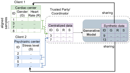
Today’s enterprises hold proprietary business-sensitive data and seek collaborative solutions for knowledge discovery while safeguarding privacy. For example, cardiologists and psychiatrists gather patients’ heart rates and mental stress levels, respectively, for potential joint treatments [1]. However, privacy regulations like GDPR [2] restrict sharing such cross-silo datasets, i.e., feature-partitioned or vertically-partitioned datasets, across enterprises. Yet, their importance in data management beckons novel solutions to learn over vertically-partitioned data silos [3, 4, 5].
In this regard, the database community is looking towards using synthetic data as an alternative to real data for protecting privacy [6, 7, 8, 9]. The current tabular generative models encompass technologies ranging from autoencoders [10, 11], flow-based models [12], autoregressive (AR) models [13], score-based models [14], Generative Adversarial Networks (GANs) [9, 15, 16, 17, 18], and the state-of-the-art diffusion models [19, 20, 21]. Recent findings show that diffusion models excel over previous technologies, including the dominant GAN-based approaches [19, 22]. This may stem from GANs’ training instability, resulting in mode-collapse and lower sample diversity compared to diffusion models [23]. Despite their promise, extending diffusion models to cross-silo data requires centralizing data at a trusted party before synthesis, as shown in Fig. 1. This violates the constraint of having data on-premise, defeating the purpose of privacy preservation.
Cross-silo methods using federated learning [24, 25] already exist for GANs [17, 16]. These are based on centralized models, such as Table-GAN [9], CTGAN [15], and CTAB-GAN [18]. However, diffusion-based cross-silo solutions do not exist despite their promising results over GANs. Therefore, we tackle the research problem of designing and training high-quality tabular diffusion synthesizers for cross-silo data.
Developing a cross-silo tabular synthesizer poses several challenges. First, tabular data has a mix of categorical and continuous features that require encoding for training. The mainstream one-hot encoding[19, 21] for categorical variables increases the difficulty in modeling distributions due to expanded feature sizes and data sparsity, and provides poor obfuscation to sensitive features. Second, for synthetic data to resemble the original distributions, capturing cross-silo feature correlations is needed. However, learning the global feature correlation is challenging without having access to a centralized dataset. Third, training on data spread across silos is expensive due to the high communication costs of distributed training. Traditional methods, such as model parallelism[26, 27], split the model across multiple clients/machines, incurring high communication overhead due to the repeated exchange of forward activations and gradients between clients.
Given these challenges, we design, \algo, a novel framework with a tabular synthesizer architecture and an efficient distributed training algorithm for feature-partitioned data. Motivated by the recent breakthrough of diffusion models in generating high-quality synthetic data using latent encodings [28], the core of \algois a latent tabular synthesizer. First, autoencoders encode sensitive features into continuous latent features. A generative Gaussian diffusion model [20] then learns to create new synthetic latents based on the latent embeddings of the original inputs. By merging latent embeddings during training, the generative model learns global feature correlations in the latent space. These correlations are maintained when decoding latents back into the real space. As a result, \algogenerates new synthetic features while keeping the original data on-premise.
incorporates multiple novelties. First is the architecture and training paradigm for the tabular synthesizer. Autoencoders and the diffusion model are trained separately in a stacked fashion, with the latent embeddings being communicated to the diffusion backbone only once. This keeps communication rounds at a constant regardless of the number of training iterations for the generator and the autoencoders. Second, our design allows the synthetic data to be generated while retaining the vertical partitioning. This has stronger privacy guarantees compared to existing cross-silo generative schemes that centralize synthetic data [17, 16]. Third, we further develop a benchmark framework to evaluate \algoand other baselines regarding the synthetic data quality and its utility on downstream tasks. Theoretical guarantees show the impossibility of data reconstruction under vertically partitioned synthesis, and risks are quantified when synthetic data is shared. Extensive evaluation on nine data sets shows that \algois competitive against centralized methods while efficiently scaling with the number of training iterations.
Contributions. \algois a novel distributed framework for training latent tabular diffusion models on cross-silo data. It’s novel features make the following contributions.
-
•
A latent tabular diffusion model that combines autoencoders and latent diffusion models. We unify the discrete and continuous tabular features into a shared continuous latent space. The backbone latent diffusion model captures the feature correlations across silos by centralizing the latents.
-
•
A stacked training paradigm that trains local autoencoders at the clients in parallel, followed by latent diffusion model training at the coordinator/server. Decoupling the training of the two components lowers communication to a single round, overcoming the high costs of end-to-end training.
-
•
A benchmarking framework that computes a resemblance score by combining five statistical measures and a utility score by comparing the downstream task performance. We also prove the impossibility of data reconstruction when the synthetic data is kept vertically partitioned and quantify the privacy risks of centralizing synthetic data using three attacks.
II Background and problem definition
In this section, we commence with the background on tabular diffusion models, focussing on the current state-of-the-art centralized synthesizer, TabDDPM [19]. We then formally define the problem setting for cross-silo tabular synthesis, identify existing research gaps, and elucidate the limitations of current centralized methods in addressing this challenge.
II-A Background: Diffusion models for tabular data synthesis
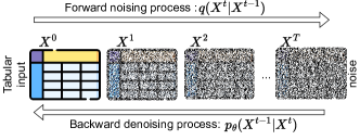
Denoising diffusion probabilistic models (DDPMs) generate data by modeling a series of forward (noising) and backward (denoising) steps, as a Markov process [20]. Fig. 2 depicts tabular synthesis with this scheme. A dataset , has samples and features. It produces a noisy dataset over noising steps. The reverse process iteratively denoises to obtain a clean dataset .
As tabular data contains both continuous and categorical features, it requires different encoding and noising/denoising methods, which we describe below. Table I summarises the mathematical notations used.
Continuous features. The forward noising transitions, , as shown in Fig. 2, gradually noise the dataset over several steps. Each transition is modeled as a normal distribution, using a variance schedule with fixed constants [20]. Through a reparameterization trick mentioned in Ho et al. [20], the forward transition for a sequence of steps can be done in a single step:
| (1) |
Here, the function obtains the noisy samples after forward steps, , and is a base noise level.
The reverse transitions , are modelled using a neural network with parameters . It learns these denoising transitions by estimating the noise added, quantified using the mean-squared-error (MSE) loss [20]:
| (2) |
Here, predicts the base noise from the noised features at step . By minimizing this loss, the neural network reduces the difference between the original inputs and the denoised outputs. Predicting the added noise brings the denoised outputs closer to the actual inputs. Hence, (2) can be viewed as minimizing the mean-squared-error (MSE) loss between the inputs and denoised outputs.
Discrete features. Working with categorical and discrete features requires Multinomial DDPMs [21]. Suppose the dataset’s -th feature, i.e., , is a categorical feature with a one-hot embedding over choices. Adding noise over its available categories changes this feature during the forward process. At each step, the model either picks the previous choice or randomly among the available categories, based on the constants [21]. This way, it gradually evolves while considering its history. The multinomial loss, denoted as , measures the difference between () and , in terms of the Kullback-Leibler divergence. Averaging the losses over all categorical features produces the final loss.
The combined loss of TabDDPM from the continuous and categorical losses is as follows:
| (3) |
Here, denotes the index set of the categorical features.

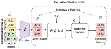
Example II.1
Consider Fig. 3, where discrete features for a sample such as gender (M/F) and marital status (single, divorced, married) are one-hot encoded as and respectively. This encoding expands the feature size of a single discrete column to 2 and 3 columns, respectively. Other continuous features with values 0.23, -0.03, and -0.91 may also be present. Using a combination of multinomial and continuous (Gaussian) DDPMs, the model noises the inputs using forward process and then denoises (using backbone ) over multiple timesteps , giving outputs . Intuitively, the model minimizes the difference between the reconstructed output and the original inputs by predicting the added noise. Mathematically, this combines the multinomial and diffusion losses using (3).
II-B Problem Definition: Cross-silo tabular synthesis
Input. In the considered scenario, there exist M distinct parties or clients . Each party possesses a subset of features , where is the total number of samples and is the number of features owned by client . These originate from a feature-partitioned dataset , with samples and features that is spread across multiple silos: , where represents column-wise concatenation. All the features are assumed to have aligned samples (rows) with other clients. This means only the rows corresponding to the common samples are selected, as shown in Fig. 1. Private-set intersection schemes achieve this through a common feature such as a sample ID [29, 30]. Without loss of generality, we assume party is the coordinator and holds the generative diffusion model .
Objective. The primary objective is to generate a synthetic dataset whose distribution is close to that of the original features while maintaining the privacy of their actual values. Each client , possesses the partition with synthetic features corresponding to their respective features while maintaining the sample alignment across clients. After generation, the feature sets can be kept vertically partitioned or shared with other clients for downstream tasks.
Constraints and Assumptions. Due to the sensitive nature of each client’s original features, they are considered confidential and, therefore, cannot be directly shared with other participants in plaintext. In other words, the original feature data that is vertically partitioned stays on the client’s premise. Moreover, we assume all parties are honest-but-curious or semi-honest [29]. This implies that all participants (including the server) follow the training and synthesizing protocols, but can attempt to infer others’ private features solely using their own data and any information communicated to them. Also, malicious behavior, like violating the protocols or feeding false data, is prohibited.
II-C Research gaps
Several reasons make the cross-silo scenario challenging to centralized tabular DDPM methods.
First, methods such as TabDDPM [19] and multinomial diffusions [21] require categorical features to be one-hot encoded. This induces sparsity and increases feature sizes, as explained in Example II.1 and Fig. 3. This can lead to complications, as the increased feature complexity increases the chances of overfitting.
Second, naively extending such methods using model-parallism [26] incurs high communication costs. For methods such as TabDDPM to be amenable to cross-silo dataset scenarios, clients must encode their local features into latents, which are then sent to the coordinator holding the generative backbone . As seen in Fig. 3, this would involve sending one-hot encodings to the backbone model held by the coordinator, which becomes more expensive due to the feature size expansion. We later show the increase in feature sizes due to one hot encoding in Table II, under Section V. Moreover, training requires end-to-end backpropagation with multiple communication round-trips between the coordinator and the clients. This scales poorly with increasing training iterations as the clients and the coordinator must exchange gradients and forward activations for every iteration.
Third, from the privacy front, centralized tabular synthesizers do not consider the risks associated with sharing synthetic features with other parties in cross-silo scenarios. As we explain in Example II.2, links between synthetic features could allow parties to model the dependencies and reconstruct private features of the other parties, posing a risk. Additionally, implementing end-to-end training in a distributed setting requires communicating gradients across parties. This increases susceptibility to attacks that exploit gradient-leakage for inferring private data [31, 32, 33].
Example II.2
Consider a scenario where Company A possesses personal information about individuals, such as names and addresses. At the same time, Company B has individuals’ financial data, such as income and spending habits. By sharing synthetic features, an adversary might detect links between certain financial behaviors and specific names or addresses. The attacker could infer or deduce patterns linking financial behaviors to specific individuals or households as synthetic features could unintentionally mirror the actual data.
III \algo
This section presents our framework \algo, with a distributed architecture for latent tabular DDPMs. We first explain the intuition and novelty of our framework, followed by an overview of the architecture, training, synthesis, and privacy analysis.
trains latent DDPMs [28], using autoencoders to encode real features into latent embeddings. The coordinator concatenates these to generate synthetic latents using the DDPM backbone (illustrated in Fig. 4). Local decoders at the clients then transform the outputs to the real space without the coordinator accessing the real features.
| Variable | Description |
| Forward noising process | |
| Original dataset, latent dataset at step 0 | |
| , | Dataset, latent dataset at -th noising step |
| -th feature of dataset | |
| , | Original and denoised -th sample at timestep |
| , | Input and denoised -th latent sample at timestep |
| Timestep, Max number of timesteps | |
| Number of samples, real feature size, latent feature size | |
| Variance schedule at timestep , and | |
| Neural network parameters, reverse process, estimated noise | |
| Continuous loss, multinomial loss at timestep | |
| Base noise level | |
| -th client | |
| Forward process output after timesteps | |
| Original features, latent features of -th client | |
| Denoised original features of -th client | |
| Denoising backbone, encoder, and decoder at -th client | |
| Centralized denoised latents, Denoised latents for |
This allows for the novelty of decoupling the training of autoencoders and the DDPM, capturing cross-silo feature correlations within the latent space without real data leaving the silos.
III-A Why the shift to latent space?
Latent DDPMs have several advantages over operating on the real space directly. Firstly, they use encoders to convert both categorical and continuous features into continuous latents, reducing sparsity and size compared to one-hot encodings (Fig. 5). This is quantitatively shown later in Table II, with one-hot encoding increasing feature sizes by nearly 10 to 200 times on some datasets. Secondly, the training phases of the autoencoder(s) and the diffusion model are decoupled/stacked, thus reducing communication costs to just one round. In contrast, the end-to-end distributed scheme jointly trains both components, increasing the cost with the number of iterations.
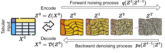
has a two-step training process. For a centralized dataset , an encoder transforms into a latent representation , where ( represents the latent space’s feature size). Subsequently, a decoder minimizes the reconstruction loss to find optimal parameters for the autoencoder.
| (4) |
Here, the loss function is chosen as negative log-likelihood or KL divergence. The coordinator then trains the diffusion model on the latents. The objective function is similar to (2) to minimize the gap between the denoised outputs and the original inputs. Hence, the function simplifies to the MSE loss between the input latents and the noisy latents :
| (5) |
Here, returns the denoised version of the samples using the backward process. The noisy latents , are computed using the forward process , as described in Section II-A.
III-B \algooverview: Distributed latent diffusion
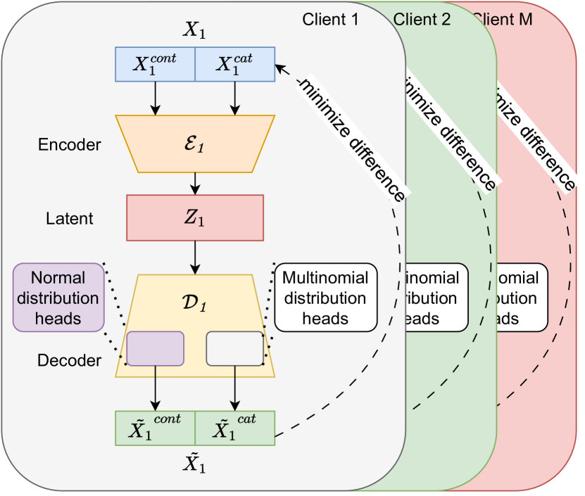
Architecture and functionalities. The model architecture of \algois depicted in Fig. 6. Each client , trains a local autoencoder, i.e., encoder-decoder pair (), which are privately held. The coordinator holds the generative diffusion model . Without loss of generality, we assign this role to .
The true features, , consist of categorical features and continuous features , as shown in Fig. 6(a). The encoders convert these features to continuous latents: . Like the original space, the latent dimensions, , sum up to give the total latent dimension, i.e., . The decoders then convert these latents features back into the original space, i.e., . Similar to tabular variational autoencoders (VAEs) [11, 15], each decoder’s head outputs a probability distribution for each feature. A typical choice for continuous features, , is the Gaussian distribution where the head outputs the mean and variance parameters to represent the spread of feature values.
A multinomial distribution head is used for categorical or discrete features, , giving probabilities for the different categories or classes.
After training the autoencoders, the encoded latents () centralize at the coordinator (see Fig. 6(b)). These undergo forward noising via function , resulting in . The backward denoising produces . Training a standard Gaussian DDPM on the continuous latents () using MSE (5), eliminates the need for a separate multinomial loss. Centralizing latents instead of actual features enables the model to learn cross-silo feature correlations within the latent space, which are preserved in the original space upon decoding.
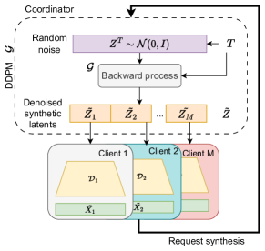
In synthesis, a client requests the coordinator to synthesize new samples (refer to Fig. 7). The coordinator begins by sampling random noise . This is then denoised over several timesteps , producing . Each client, , receives a part of the synthetic latents, i.e., . Using their private decoder , clients convert these into the original space, i.e., . This generates feature-partitioned synthetic samples while preserving inter-feature associations.
IV \algo: Distributed Training and Synthesis
In this section, we describe the algorithms for training and synthesis and discuss the privacy implications in \algo. We provide theoretical arguments for privacy based on latent irreversibility for vertically partitioned synthesis. We also indicate the risks of sharing features post-generation.
IV-A Distributed Training
’s training process adopts a stacked two-step approach, departing from standard end-to-end training. Fig. 6 illustrates the two-step procedure detailed in Algorithm 1.
Individual Autoencoder Training (lines [1-1] of Algorithm 1): For input sample features , client converts all features into numerical embeddings, employing one-hot encoding for categorical features. These continuous and categorical embeddings pass through an MLP of an encoder (), producing continuous-valued latents . A decoder processes these latents, using output heads to map each feature to a normal or categorical distribution akin to other tabular VAEs [11, 15]. The loss function (4), measures the logarithm of the probability density between the output distributions and input features, for both categorical and discrete features.
Generative Diffusion Model Training: After training the autoencoders, each client produces latent features of the original training samples, i.e., , and communicates these to the coordinator. The coordinator concatenates these to obtain ((lines 1,1)).
The coordinator then trains locally for multiple epochs. It samples random base noise level and timesteps at each epoch and performs the forward noising process . It then internally predicts the noise level added during the forward process to update the generator for modeling the backward process (lines 1-1).
IV-B Distributed Synthesis
The DDPM backbone and local decoders at each client are stacked for post-training synthesis, detailed in Algorithm 2.
Upon receiving a client’s request, the coordinator samples Gaussian noise (line 2). Over multiple iterations in , noise is removed, yielding . Clients then use their local decoder to translate their partition of the latent samples into real samples . Links between are preserved in due to the centralization of latents during training.
IV-C Privacy in training
The localized training of autoencoders and the diffusion model ensures that sensitive information remains confined within each client’s domain. Despite sharing latent embeddings with the coordinator, the absence of decoders at the coordinator prevents data reconstruction from the latents. The coordinator aggregates latents to capture cross-client feature associations without observing the original features, thereby preserving privacy.
Crucially, at no point during the training phase are raw, identifiable features shared. Instead, the communication revolves around derived latent representations or aggregated latent spaces, mitigating the risk of sensitive information exposure. Access to the decoders is necessary to revert latents to the real space. But as they are privately held, access is restricted, preventing the reversion process.
IV-D Privacy in synthesizing
In our formulation, synthesis occurs in two scenarios. In the first case, the synthesized data remains vertically partitioned, with each client retaining only their respective features post-generation. In the second case, parties may share their synthetic features after generating them. While the latter allows parties to model downstream tasks independently, it introduces privacy risks due to links between features, as explained in example II.2. In contrast, the first case offers stronger guarantees by restricting access to other parties’ features. However, it requires collaborative methods like vertical federated learning [34, 29, 35] for modeling downstream tasks, incurring a higher cost.
When features are shared, privacy guarantees become weaker, and we resort to empirical risk estimation, as shown in Section V-. But for the first case, reconstructing inputs from just latents is challenging for the coordinator, as it is akin to finding the encoding function’s inverse without knowing the inputs or the function itself. While intuitive, we formalize this here. Lemma 1 shows the impossibility of data reconstruction without knowing the domain of the inputs. Lemma 2 extends the impossibility result to cases where the domain is known but requires a domain with at least two elements. Both are building blocks for the latent irreversibility theorem of \algo.
Lemma 1: For any function , where is the codomain (latent space), there exists no oracle function capable of uniquely identifying the domain (input space) without knowledge of the function .
Proof: For the sake of contradiction assume there is an oracle capable of identifying the domain without knowledge of . However, since there are infinitely many possible domains that can map to a given codomain , the oracle cannot uniquely map elements of to the correct domain.
Therefore, such an oracle cannot exist.
Lemma 2: For any surjective function , where has more than one element, there does not exist an oracle capable of uniquely identifying the pre-image111Pre-images with cardinality one: https://mathworld.wolfram.com/Pre-Image.html of any element in without knowledge of .
Proof: Assume, for contradiction, the existence of an oracle capable of identifying the pre-image of any element in without knowledge of . We consider two cases:
-
1.
If is not injective, then at least one element has multiple pre-images in . This ambiguity makes it impossible for to uniquely identify a single pre-image for , contradicting the existence of .
-
2.
If is injective, we can construct another function by swapping the mappings of two distinct elements in (i.e., and ). This keeps the same codomain yet introduces ambiguity in determining the right pre-image without explicit knowledge of the function used, i.e., or . This scenario again contradicts the oracle’s supposed capability to identify a unique pre-image.
Therefore, such an oracle cannot exist.
Theorem 1 (Latent irreversibility):
In the \algoframework with private data (from input space ) and privately-held encoder and decoder functions (), the coordinator/server cannot reconstruct real samples from latent encodings alone when the domain is unknown. Reconstruction remains impossible if the domain is known and its size is greater than one.
Proof: Suppose, for contradiction, that the server can reconstruct real samples from just the latents. This implies the existence of an oracle , from the latent space to the real space .
We consider two cases based on Lemmas 1 and 2:
-
1.
Case 1: Without knowing the encoding/decoding functions or the domain of , the server cannot uniquely identify the real samples from the latents alone. In this case, Lemma 1 applies, so such an oracle cannot exist.
-
2.
Case 2: If the domain is known, the server cannot reconstruct real samples from just the latents. In this case, Lemma 2 applies, so the oracle cannot exist.
Since both cases lead to contradictions, we conclude that the coordinator cannot reconstruct real samples from the latents alone in \algo’s framework.
V Experiments
We assess \algo’s performance on multiple aspects. First, we evaluate its synthetic data quality against centralized and decentralized methods, considering its resemblance to original data and utility in downstream tasks. Second, we compare \algo’s communication costs with end-to-end training, highlighting the reduced costs of stacked training. Third, we analyze \algo’s privacy risks when sharing synthetic features post-generation. We also test \algo’s robustness to feature permutation under a varying number of clients and partition sizes222Full experimental results available here: https://www.dropbox.com/scl/fo/carrcdl9v13b2813e58ui/h?rlkey=vakpjh83xt2ui6o8r51xljm32&dl=0.
V-A Experiment Setup
Hardware & Software. We run experiments on an AMD Ryzen 9 5900 12-core processor and an NVIDIA 3090 RTX GPU with CUDA version 12.0. The OS used is Ubuntu 20.04.6 LTS. PyTorch is used to simulate the distributed experiments by creating multiple models corresponding to individual clients.
Datasets. To assess the quality of generated data, we use nine benchmark datasets used in generative modeling: Abalone [36], Adult [37], Cardio [38], Churn Modelling [39], Cover [40], Diabetes [41], Heloc, Intrusion [42], and Loan [43]. These are well-known benchmarks in the context of generative modeling [18, 19].
| #Rows | #Cat. | #Num. | #Bef. | #Aft. | Incr. | |
| Loan | 5000 | 7 | 6 | 13 | 23 | 1.77x |
| Adult | 48842 | 9 | 5 | 14 | 108 | 7.71x |
| Cardio | 70000 | 7 | 5 | 12 | 21 | 1.75x |
| Abalone | 4177 | 2 | 8 | 10 | 39 | 3.9x |
| Churn | 10000 | 8 | 6 | 14 | 2964 | 211.71x |
| Diabetes | 768 | 2 | 7 | 9 | 26 | 2.89x |
| Cover | 581012 | 45 | 10 | 55 | 104 | 1.89x |
| Intrusion | 22544 | 22 | 20 | 42 | 268 | 6.38x |
| Heloc | 10250 | 12 | 12 | 24 | 239 | 9.96x |
From Table II, we can classify the datasets into three categories based on the number of features: i. Easy - Abalone, Diabetes, Cardio. ii. Medium - Adult, Churn, Loan. iii. Hard - Intrusion, Heloc, Cover. Table II also includes the total feature sizes before and after one hot encoding and their corresponding changes (used by TabDDPM and GANs).
Baselines. We tested centralized tabular GAN methods [18, 15, 9] falling under two architectural flavors: linear backbone, i.e., CTGAN (GAN(linear)) [15], and convolutional backbone, i.e., CTAB-GAN (GAN(conv)) [18], which extends CTGAN and Table-GAN [9]. For DDPMs, the models compared are tabular latent-diffusion models, \algo, and its centralized counterpart LatentDiff. In addition, we also compare these models with their corresponding end-to-end trained versions, i.e., centralized E2E (end-to-end centralized) and distributed E2EDistr (end-to-end distributed), with architectures as shown in Fig. 8 and Fig. 9 respectively. State-of-the-art TabDDPM is also compared.
| Model | Abalone | Adult | Cardio | Churn | Cover | Diabetes | Heloc | Intrusion | Loan |
| GAN(conv) | 64.0 0.00 | 38.0 0.00 | 59.8 0.40 | 43.4 0.80 | 45.2 0.40 | 75.8 0.40 | 54.0 0.00 | 47.2 0.40 | 76.4 0.49 |
| GAN(linear) | 54.2 0.40 | 28.6 0.49 | 29.0 0.00 | 30.8 0.39 | 36.0 0.00 | 51.0 0.00 | 48.0 0.00 | 39.0 0.00 | 40.0 0.00 |
| E2E | 85.20.40 | 60.00.00 | 60.20.40 | 88.20.40 | 51.00.40 | 72.40.80 | 68.40.49 | 48.0 0.00 | 81.20.40 |
| E2EDistr | 56.40.80 | 46.01.09 | 44.00.89 | 78.00.00 | 40.80.40 | 61.8 3.12 | 61.00.00 | 37.00.00 | 49.81.16 |
| TabDDPM | 91.20.75 | 97.00.00 | 98.00.00 | 63.60.49 | 78.00.00 | 94.60.49 | 88.00.00 | 44.00.00 | 98.00.00 |
| LatentDiff | 92.00.00 | 78.00.00 | 72.20.40 | 89.00.00 | 92.00.00 | 90.00.63 | 83.40.49 | 68.00.00 | 83.40.49 |
| \algo | 91.00.00 | 73.00.00 | 71.00.00 | 87.00.00 | 89.0 0.00 | 84.00.63 | 79.00.00 | 67.00.00 | 81.20.40 |
| PPD (vs GAN) | 27.0 | 35.0 | 11.2 | 43.6 | 43.8 | 8.2 | 25.0 | 19.8 | 4.8 |
| Model | Abalone | Adult | Cardio | Churn | Cover | Diabetes | Heloc | Intrusion | Loan |
| GAN(conv) | 71.0 0.63 | 82.6 11.30 | 94.0 3.63 | 85.0 1.09 | 82.6 1.01 | 96.2 2.56 | 45.0 0.63 | 36.2 0.98 | 82.6 0.49 |
| GAN(linear) | 65.2 0.40 | 30.6 1.62 | 47.6 0.49 | 78.4 1.02 | 36.2 0.40 | 84.6 1.62 | 38.4 0.49 | 25.4 0.49 | 82.0 0.63 |
| E2E | 70.01.41 | 45.01.67 | 75.21.47 | 87.80.74 | 89.80.40 | 84.25.11 | 39.80.40 | 31.00.63 | 77.00.89 |
| E2EDistr | 70.81.72 | 33.61.02 | 55.30.33 | 87.00.89 | 56.81.46 | 89.02.28 | 39.20.40 | 24.21.16 | 71.22.92 |
| TabDDPM | 98.40.49 | 89.21.60 | 99.60.49 | 44.46.28 | 80.47.94 | 100.00.00 | 96.40.49 | 23.04.98 | 98.81.17 |
| LatentDiff | 100.00.00 | 100.00.00 | 86.42.33 | 100.00.00 | 95.80.40 | 99.60.49 | 76.40.49 | 61.21.16 | 94.81.93 |
| \algo | 97.21.16 | 96.65.04 | 93.24.95 | 90.40.49 | 96.40.49 | 95.23.92 | 74.80.74 | 64.20.74 | 90.00.89 |
| PPD (vs GAN) | 26.2 | 14.0 | -0.8 | 5.4 | 13.8 | -1.0 | 29.8 | 28.0 | 7.4 |
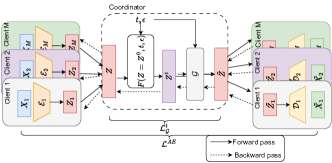
The architectures of E2E and E2EDistr, shown in Fig. 8 and Fig. 9 respectively, consist of an encoder followed by the DDPM and a decoder at the end. During training, the encoder(s) first compute(s) latents. The DDPM unit adds noise and iteratively denoises it to generate synthetic latents. The decoder(s) then recover the output in the original space and compute the losses individually using (4). The MSE loss from the DDPM component is added (5), and the entire network is trained end-to-end.
Training configurations. For \algo, LatentDiff, E2E, and E2EDistr models, we utilize an autoencoder architecture with three linear layers for encoders and decoders. The activation function used is GELU [44]. In centralized versions, the embedding and hidden dimensions are set to 32 and 1024, respectively, equally partitioned between clients in the distributed versions. The latent dimension is set to the number of original features before one-hot encoding. In the case of distributed models (\algo, E2EDistr), the centralized autoencoders are evenly split across different clients. However, for TabDDPM, which lacks autoencoders, a 6-layer MLP with a hidden dimension of 256 forms the neural backbone of its DDPM. For the remaining models, a neural backbone for the DDPM consists of a bilinear model comprising eight layers with GELU activation and a dropout factor of 0.01. For the GAN baselines, we use four convolutional or linear layers with leaky ReLU activation and layer norm for the generator. The discriminator uses the transposed architecture but is otherwise similar. All models are trained for 500,000 iterations encompassing the autoencoders and the DDPM’s neural network, using a batch size 512 and a learning rate of 0.001. DDPM training involves a maximum of 200 timesteps, with inference conducted over 25 steps. In the case of distributed models (\algoand E2EDistr), dataset features are partitioned equally among four clients. The last client gets any remaining features post-division without shuffling.
V-B Benchmark Framework
uses three types of metrics for the evaluation: resemblance, utility, and privacy. All metrics are in the range of (0-100), with 100 being the “best”. The quality of synthetic data is calculated using resemblance and utility. Privacy metrics quantify the leakage associated with centralizing the synthetic features post-generation. We explain these metrics in detail as follows.
Resemblance measures how close the synthetic data is to the original data regarding feature distributions. It is a composite score that considers similarities between the real and synthetic data by computing the mean of the following five scores:
- 1.
-
2.
Correlation Similarity: The correlation between the correlation coefficients between each pair of columns using pairwise Pearson correlation and Theil’s U for numerical and categorical features, respectively.
-
3.
Jensen-Shannon Similarity [47]: This computes the distance between the probability distributions of the real and synthetic columns. One minus the distance is used so that all metrics are comparable, with higher scores being better.
-
4.
Kolmogorov-Smirnov Similarity [48]: This distance measure computes the maximum difference between cumulative distributions of each real and synthetic feature. One minus the distance makes higher scores better.
-
5.
Propensity Mean-Absolute Similarity [49]: A binary classifier (XGBoost [50]) is trained to discriminate between real and synthetic samples. When the classifier cannot distinguish between the two datasets, the mean-absolute error of its probabilities is 0. One minus the error is used so that higher scores are better.
Utility measures how the synthetic data performs on a downstream prediction task using an XGBoost model. Real or synthetic datasets are used for training, and evaluation is done using the same real hold-out set in each case. The downstream performance is calculated by taking the 90th percentile of macro-averaged F1 scores for categorical columns and the D2 absolute error scores for continuous columns. Finally, the utility score is calculated by taking the ratio of the synthetic to the real data’s downstream performance (in percent, clipped at the max value of 100).
Privacy quantifies the risk associated with sharing the synthetic features post-generation by averaging the scores from three attacks based on the framework in [51] and [52]. Again, higher scores indicate better resistance against the following three attacks.
-
1.
Singling Out Attack [51]: This singles out individual data records in the training dataset. If unique records can be identified, the synthetic data might reveal individuals based on their unique attributes.
-
2.
Linkability Attack [51]: This associates two or more records, either within the synthetic dataset or between the synthetic and original datasets, by identifying records linked to the same individual or group.
-
3.
Attribute Inference Attack [52]: This deduces the values of undisclosed attributes of an individual based on the information available in the synthetic dataset.
V-C Quantitative analysis
Setup. We quantitatively analyze the resemblance and utility scores on the nine diverse datasets (abalone, adult, cardio, cover, churn_modelling, diabetes, heloc, intrusion, and loan). The models compared are \algo, GANs (GAN(linear), GAN(conv)), centralized latent diffusion (LatentDiff), end-to-end baselines (E2E, E2EDistr), and TabDDPM. Four clients were used for the distributed models (\algoand E2EDistr). The resemblance and utility scores (0-100) are averaged from 5 trials, results for which are shown in Table III and Table IV.
| \algo | LatentDiff | TabDDPM | |
|
Cardio |
![[Uncaptioned image]](/html/2404.03299/assets/x11.png) |
![[Uncaptioned image]](/html/2404.03299/assets/x12.png) |
![[Uncaptioned image]](/html/2404.03299/assets/x13.png) |
|
Intrusion |
![[Uncaptioned image]](/html/2404.03299/assets/x14.png) |
![[Uncaptioned image]](/html/2404.03299/assets/x15.png) |
![[Uncaptioned image]](/html/2404.03299/assets/x16.png) |
Comparable model performance to centralized methods. Coinciding with the results of other works [22, 19], we see that our decentralized latent diffusion method significantly outperforms centralized GANs. Improvements of up to 43.8 and 29.8 percentage points are achieved over GANs on resemblance and utility. This could be due to instabilities with training GANs leading to mode collapse [23]. As a result, the generator may end up oversampling cases that escape the notice of the discriminator, leading to low diversity. Within DDPMs, TabDDPM’s and LatentDiff’s performance are generally an upper bound to what \algocan achieve since they are centralized baselines. Despite this, \algoachieves comparable resemblance and utility scores, especially compared to its centralized version LatentDiff. Interestingly, the end-to-end versions E2E and E2EDistr perform the worst. This may be because the DDPM backbone at the intermediate level needs to add noise to the latents and then denoise them during training. This may be problematic, especially during the initial training phases, as the received latents are already quite noisy since the autoencoders are initially untrained. Therefore, noise is added to more noise, making it difficult to distinguish the ground truth from actual noise. On the other hand, with \algoand LatentDiff, the noise needs to be removed from fully-trained autoencoders. So, the latent values are less noisy, making it easier for the DDPM to distinguish between noise and actual latents during training correctly.
Result analysis. We generally observe that latent DDPMs are better performing than TabDDPM on challenging datasets with a lot of sparse features, such as Intrusion and Cover, whereas TabDDPM does better on more straightforward datasets with a smaller number of features, such as Loan, Adult, and Diabetes. This indicates that combining multinomial and MSE loss may be better for high-quality data generation with low feature sizes and sparsity. At the same time, the conversion into latent space may be better for highly sparse datasets with large cardinality in discrete values.
V-D Qualitative Analysis
Setup. We qualitatively analyze the generated synthetic data based on the feature correlation differences between the real and synthetic features. Based on the resemblance and utility scores from Table III and Table IV, we select the top three models (TabDDPM, LatentDiff, and \algo) and show the correlation difference graphs for one of the simpler datasets (Cardio) and one hard dataset (Intrusion). Again, four clients were used for \algo333Additional results on feature distributions of real and synthetic data are available in the appendix: https://www.dropbox.com/scl/fi/lq01y9qbbzbvaqnh7owva/SiloFuse_appendix.pdf?rlkey=ed0bf2lb8pmc9g4siey665s3b&dl=0.
High correlation resemblance of \algo. The graphs in Table V show that \algocaptures feature correlations well and is comparable to the centralized version, i.e., LatentDiff’s performance. It also performs better than TabDDPM on the harder dataset, Intrusion, as we see a darker shade for the correlation differences for TabDDPM. However, we observe that TabDDPM performs better on the simpler dataset, Cardio, due to the lower difference. These results match the scores indicated in Table III and Table IV. As explained earlier, the large feature size of Intrusion makes it more challenging to model. It is amplified in difficulty for TabDDPM due to the additional sparsity induced by one-hot encoding. This makes it do worse than the latent space models. On Cardio, the problem of sparsity is not amplified by a lot as the number of discrete features is lower, enabling TabDDPM to perform better. Nevertheless, \algodoes not perform much worse than TabDDPM even on Cardio, as the correlation differences are not very large.
| Model | Abalone | Adult | Cardio | Churn | Cover | Diabetes | Heloc | Intrusion | Loan |
| TabDDPM | 48.20.48 | 70.12.61 | 76.12.19 | 86.70.24 | 59.13.85 | 46.20.69 | 56.71.60 | 92.12.62 | 57.91.87 |
| LatentDiff | 50.3 0.58 | 73.7 2.29 | 88.7 2.82 | 78.1 4.18 | 55.7 1.81 | 62.4 1.32 | 51.9 1.46 | 70.5 2.89 | 64.8 2.36 |
| \algo | 55.90.46 | 92.10.60 | 93.24.97 | 92.31.84 | 65.12.25 | 78.12.40 | 56.41.58 | 70.52.46 | 79.35.35 |
V-E Communication Efficiency
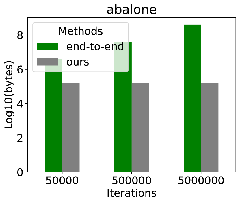
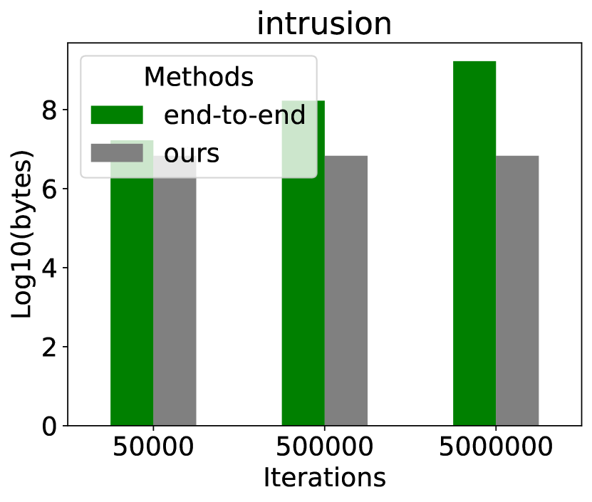
Setup. To demonstrate the benefits of stacked training over end-to-end training with increasing iterations, we compare \algowith E2EDistr, using the same parameter sizes for the autoencoders and the DDPM’s neural backbone in each. Again, we use four clients with equally partitioned features. The iterations are varied between 50,000, 500,000, and 5 million. We measure the total bytes transferred between the clients and the coordinator over the course of the training process. Without loss of generality, we show the results on two datasets. One simple dataset with fewer features, i.e., Abalone, and one difficult dataset, Intrusion.
Constant communication cost of \algo. From Fig. 10, we see that changing the number of iterations does not increase the communication cost of \algo. Due to the stacked training, the latents for the original training data only need to be transferred to the coordinator once after training autoencoders on each client. As the autoencoders and the DDPM are trained independently, there is no requirement to communicate gradients and forward activations between clients repeatedly, which results in a single round. End-to-end training methods such as TabDDPM, E2E, and E2EDistr thus suffer from increasing costs as the iterations increase, i.e., they have cost . Naively distributing TabDDPM would incur even higher costs than E2EDistr, as one-hot encoding significantly increases the feature sizes being communicated (see Table II). As shown in the table, some datasets have a significant increase in size, leading to a proportionate rise that exceeds even E2EDistr: Churn (>200x), Heloc (>9x), Adult (>7x), and Intrusion (>6x).
V-F Empirical Privacy Risk Analysis
Setup. Typically, post-generation, the synthetic data partitions from each client are shared with all parties. Although this methodology offers significant practical utility, it also poses privacy risks. Specifically, the distributions of the synthetic data could leak information on the original features, e.g., attribute inference attacks [52]. We quantify this risk by computing the privacy scores as explained in Section V-F. The best-performing methods, \algo. LatentDiff, and TabDDPM are compared again, with the results shown in Table VI.
Improved privacy against centralized baselines. From the results, we see that \algohas the overall best privacy score, indicating it runs the lowest risk of leaking private feature information post-generation. While TabDDPM and LatentDiff were able to achieve better resemblance and utility scores, we see that they lack in terms of privacy. \algoachieves higher privacy scores than the centralized version, LatentDiff, on 8 out of 9 datasets, ranging from 4.5% (Cardio, Heloc), rising to 18.4%, 15.7%, and 14.2% on Adult, Diabetes, and Churn respectively.
Privacy-quality tradeoffs. Despite the higher privacy score of \algo, there is an inherent tradeoff between achieving very high utility and resemblance versus high privacy. For example, in Intrusion data, we observe that TabDDPM achieves the highest privacy score but has significantly lower resemblance and utility. Hence, data privacy may be better, but the synthetic samples may be unusable for the downstream task. Conversely, training the generative model using centralized features allows the model to capture relations between features better, leading to higher resemblance and utility. However, having synthetic features that highly resemble original features will enable adversaries to map the associations between features better, lowering privacy. While differential privacy adds noise to synthetic data for better privacy, it can lead to performance tradeoffs that are hard to control [16, 53].
We also evaluate the sensitivity of privacy scores when the number of denoising steps varies. Two datasets were chosen: one easier dataset (abalone) and one difficult (heloc). As shown in Table VII, increasing the denoising steps allows the latent diffusion model to remove more noise, but lowers the privacy score. Notably, the privacy scores saturate quickly upon increasing the number of denoising steps. Hence, the scores lose sensitivity to the noise level within a few timesteps.
| Dataset | Inference timesteps | ||
| 2 | 5 | 25 | |
| Abalone | 58.15 0.90 | 51.6 0.41 | 50.3 0.58 |
| Heloc | 66.1 1.15 | 53.4 0.56 | 51.9 1.46 |
V-G Robustness to client data distribution
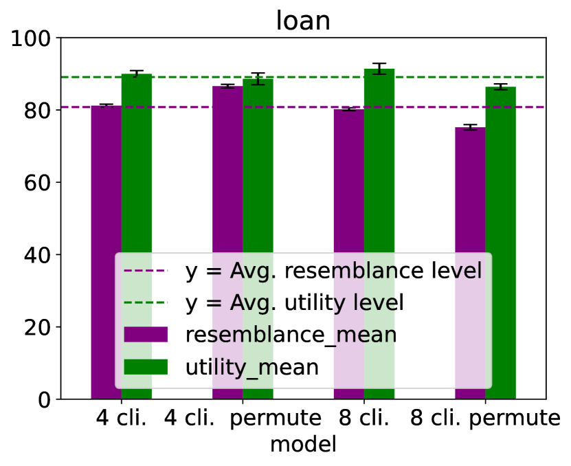
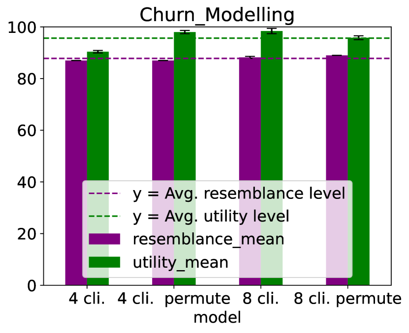
Setup. \algo’s robustness to differing partition sizes on clients and permuted feature assignments is measured. We vary the clients between 4 and 8 and also experiment with two orders of the feature assignments to clients. The first order maintains unshuffled columns. The second order shuffles the columns using a seed value of 12343. After shuffling, we partition the columns for allocation to each client. Without loss of generality, we show the results (Fig. 11) for three datasets: Heloc, Loan, and Churn. Results on additional datasets are available in the link pointing to the full experimental results (see Section V).
Robustness to feature permutation and partitioning. From the figures, we see that changing the number of clients or shuffling the features does not make the resemblance/utility deviate too much from the average level, indicating that \algois generally invariant to feature permutation. This is because centralization of the latents at the DDPM allows it to capture cross-feature correlations that may have been missed or poorly captured at the local encoders. This enables the model to achieve similar resemblance and utility scores.
Exceptions stand out in specific scenarios. For instance, resemblance notably drops in the Loan dataset transitioning from 4 to 8 clients with permuted feature assignments (Fig. 11(b)). In the Churn dataset, utility significantly improves when moving from default to permuted partitioning (Fig. 11(c)). The drop in resemblance might arise from correlated features being reassigned to different clients in the 8-client setup, delaying the learning of associations. Improved performance for the latter case may stem from separating jointly-existing noisy features during re-partitioning or permutation.
| Method | Type | Cross-silo | Tabular | Generating space |
| GTV [17] | GAN | ✔ | ✔ | Real |
| DPGDAN [16] | GAN | ✔ | ✔ | Real |
| MedGAN [10] | GAN | ✖ | ✔ | Latent |
| VQ-VAE [11] | VAE | ✖ | ✔ | Real |
| TVAE [15] | VAE | ✖ | ✔ | Real |
| dpart [13] | AR | ✖ | ✔ | Real |
| DP-HFLOW [12] | Flow | ✖ | ✔ | Real |
| STaSY [14] | Score-matching | ✖ | ✔ | Real |
| Hoogeboom et al. [21] | DDPM/Flow | ✖ | ✔ | Real |
| TabDDPM [19] | DDPM | ✖ | ✔ | Real |
| Rombach et al. [28] | DDPM | ✖ | ✖ | Latent |
| \algo | DDPM | ✔ | ✔ | Latent |
VI Related Work
Tabular Synthesizers. In the domain of generative modeling, deep neural network methods span variational autoencoders (VAEs), GANs, energy-based models (DDPMs, Score-matching), autoregressive models (AR), and flow-based methods, outlined in Bond et al. [54]. Given our focus on tabular data synthesis, our exploration centers on the techniques delineated in Table VIII, predominantly comprising tabular synthesizers. Although Hoogeboom et al.’s approach [21] pioneers multinomial DDPMs, it exclusively applies to categorical features, addressing only part of the tabular data synthesis need. Additionally, Rombach et al.’s work [28], a DDPM-based method inspiring \algo’s latent space modeling, is tailored exclusively for image data.
Cross-silo synthesis. Other than \algo, GAN-based methods, such as GTV [17] and DPGDAN [16], tackle the cross-silo challenge. Their backbones use centralized GAN architectures, i.e., Table-GAN, CTGAN, and CTAB-GAN [9, 15, 18], which \algooutperforms. They also employ end-to-end training, increasing communication costs.
End-to-end (real space) vs. stacked training (latent space). Most generative methods directly operate in the original/real space, requiring end-to-end training. In contrast, latent-based models can decouple training into local autoencoder training followed by generative modeling in the latent space. Limited work exists in this paradigm: MedGAN [10] uses an autoencoder to transform features into continuous latents, followed by a GAN-based generative step, but it is centralized and unfit for cross-silo scenarios. Rombach et al. [28] operates in the latent space solely for image data and in a centralized setup.
VII Conclusion
We introduce \algo, a distributed latent DDPM framework for cross-silo tabular data synthesis. \algotrains models collaboratively by encoding original features into a latent space, ensuring confidentiality while avoiding the high costs of mainstream one-hot encoding. We introduce a stacked training paradigm to decouple the training of autoencoders and the diffusion generator. This minimizes communication costs by transmitting latent features only once and avoids the risks of gradient leakage attacks. Centralizing latent features preserves cross-silo links while thwarting data reconstruction under vertically partitioned synthesis.
Quantitative and qualitative analyses show \algo’s comparable performance with centralized baselines regarding synthetic data quality, with diffusion-based models outperforming GANs. \algoachieves improvements of up to 43.8 and 29.8 percent points higher than centralized GANs on resemblance and utility, respectively. Stacked training reduces communication rounds to one step, significantly better than end-to-end training paradigms (). When sharing synthetic data post-generation, \algoexhibits superior resistance against attacks, with minor trade-offs in data quality. Although robust under varied scenarios, slight susceptibility to feature permutation suggests room for future improvement.
Sharing synthetic features across parties poses challenges and potential privacy vulnerabilities. Future research could explore controlled information exchange or employ trusted third-party interventions to ensure privacy in collaborative training. Exploring methods like vertical federated learning would offer ways to achieve both privacy and high performance in downstream tasks by retaining feature-partitioning.
Acknowledgment
This paper is supported by the project Understanding Implicit Dataset Relationships for Machine Learning (VI.Veni.222.439), of the research programme NWO Talent Programme Veni, partly financed by the Dutch Research Council (NWO). It is also supported by the DepMAT project (P20-22) of the NWO Perspectief programme.
References
- [1] M. De Hert, J. Detraux, and D. Vancampfort, “The intriguing relationship between coronary heart disease and mental disorders,” Dialogues in clinical neuroscience, 2022.
- [2] P. Regulation, “Regulation (eu) 2016/679 of the european parliament and of the council,” Regulation (eu), vol. 679, p. 2016, 2016.
- [3] J. Vaidya and C. Clifton, “Privacy preserving association rule mining in vertically partitioned data,” in Proceedings of the eighth ACM SIGKDD international conference on Knowledge discovery and data mining, 2002, pp. 639–644.
- [4] Jaideep Vaidya and Chris Clifton, “Privacy-preserving k-means clustering over vertically partitioned data,” in Proceedings of the ninth ACM SIGKDD international conference on Knowledge discovery and data mining, 2003, pp. 206–215.
- [5] S. Navathe, S. Ceri, G. Wiederhold, and J. Dou, “Vertical partitioning algorithms for database design,” ACM Trans. Database Syst., vol. 9, no. 4, p. 680–710, dec 1984. [Online]. Available: https://doi.org/10.1145/1994.2209
- [6] A. Sanghi and J. R. Haritsa, “Synthetic data generation for enterprise dbms,” in 2023 IEEE 39th International Conference on Data Engineering (ICDE), 2023, pp. 3585–3588.
- [7] W. Li, “Supporting database constraints in synthetic data generation based on generative adversarial networks,” in Proceedings of the 2020 ACM SIGMOD International Conference on Management of Data, ser. SIGMOD ’20. New York, NY, USA: Association for Computing Machinery, 2020, p. 2875–2877. [Online]. Available: https://doi.org/10.1145/3318464.3384414
- [8] J. Fan, J. Chen, T. Liu, Y. Shen, G. Li, and X. Du, “Relational data synthesis using generative adversarial networks: a design space exploration,” Proc. VLDB Endow., vol. 13, no. 12, p. 1962–1975, jul 2020. [Online]. Available: https://doi.org/10.14778/3407790.3407802
- [9] N. Park, M. Mohammadi, K. Gorde, S. Jajodia, H. Park, and Y. Kim, “Data synthesis based on generative adversarial networks,” Proc. VLDB Endow., vol. 11, no. 10, p. 1071–1083, jun 2018. [Online]. Available: https://doi.org/10.14778/3231751.3231757
- [10] E. Choi, S. Biswal, B. Malin, J. Duke, W. F. Stewart, and J. Sun, “Generating multi-label discrete patient records using generative adversarial networks,” in Machine learning for healthcare conference. PMLR, 2017, pp. 286–305.
- [11] A. v. d. Oord, O. Vinyals, and K. Kavukcuoglu, “Neural discrete representation learning,” arXiv preprint arXiv:1711.00937, 2017.
- [12] J. Lee, M. Kim, Y. Jeong, and Y. Ro, “Differentially private normalizing flows for synthetic tabular data generation,” in Proceedings of the AAAI Conference on Artificial Intelligence, vol. 36, no. 7, 2022, pp. 7345–7353.
- [13] S. Mahiou, K. Xu, and G. Ganev, “dpart: Differentially private autoregressive tabular, a general framework for synthetic data generation,” arXiv preprint arXiv:2207.05810, 2022.
- [14] J. Kim, C. Lee, and N. Park, “Stasy: Score-based tabular data synthesis,” arXiv preprint arXiv:2210.04018, 2022.
- [15] L. Xu, M. Skoularidou, A. Cuesta-Infante, and K. Veeramachaneni, “Modeling tabular data using conditional gan,” Advances in neural information processing systems, vol. 32, 2019.
- [16] Z. Wang, X. Cheng, S. Su, and G. Wang, “Differentially private generative decomposed adversarial network for vertically partitioned data sharing,” Information Sciences, vol. 619, pp. 722–744, 2023.
- [17] Z. Zhao, H. Wu, A. Van Moorsel, and L. Y. Chen, “Gtv: Generating tabular data via vertical federated learning,” arXiv preprint arXiv:2302.01706, 2023.
- [18] Z. Zhao, A. Kunar, R. Birke, and L. Y. Chen, “CTAB-GAN: Effective table data synthesizing,” in Asian Conference on Machine Learning. PMLR, 2021, pp. 97–112.
- [19] A. Kotelnikov, D. Baranchuk, I. Rubachev, and A. Babenko, “Tabddpm: Modelling tabular data with diffusion models,” in International Conference on Machine Learning. PMLR, 2023, pp. 17 564–17 579.
- [20] J. Ho, A. Jain, and P. Abbeel, “Denoising diffusion probabilistic models,” Advances in neural information processing systems, vol. 33, pp. 6840–6851, 2020.
- [21] E. Hoogeboom, D. Nielsen, P. Jaini, P. Forré, and M. Welling, “Argmax flows and multinomial diffusion: Learning categorical distributions,” Advances in Neural Information Processing Systems, vol. 34, pp. 12 454–12 465, 2021.
- [22] P. Dhariwal and A. Nichol, “Diffusion models beat gans on image synthesis,” Advances in neural information processing systems, vol. 34, pp. 8780–8794, 2021.
- [23] R. Bayat, “A study on sample diversity in generative models: Gans vs. diffusion models,” 2023.
- [24] T. Li, A. K. Sahu, A. Talwalkar, and V. Smith, “Federated learning: Challenges, methods, and future directions,” IEEE signal processing magazine, vol. 37, no. 3, pp. 50–60, 2020.
- [25] J. Konečnỳ, H. B. McMahan, F. X. Yu, P. Richtárik, A. T. Suresh, and D. Bacon, “Federated learning: Strategies for improving communication efficiency,” arXiv preprint arXiv:1610.05492, 2016.
- [26] J. Dean, G. Corrado, R. Monga, K. Chen, M. Devin, M. Mao, M. Ranzato, A. Senior, P. Tucker, K. Yang et al., “Large scale distributed deep networks,” Advances in neural information processing systems, vol. 25, 2012.
- [27] P. Vepakomma, O. Gupta, T. Swedish, and R. Raskar, “Split learning for health: Distributed deep learning without sharing raw patient data,” arXiv preprint arXiv:1812.00564, 2018.
- [28] R. Rombach, A. Blattmann, D. Lorenz, P. Esser, and B. Ommer, “High-resolution image synthesis with latent diffusion models,” in Proceedings of the IEEE/CVF conference on computer vision and pattern recognition, 2022, pp. 10 684–10 695.
- [29] S. Hardy, W. Henecka, H. Ivey-Law, R. Nock, G. Patrini, G. Smith, and B. Thorne, “Private federated learning on vertically partitioned data via entity resolution and additively homomorphic encryption,” arXiv preprint arXiv:1711.10677, 2017.
- [30] M. Scannapieco, I. Figotin, E. Bertino, and A. K. Elmagarmid, “Privacy preserving schema and data matching,” in Proceedings of the 2007 ACM SIGMOD international conference on Management of data, 2007, pp. 653–664.
- [31] X. Jin, P.-Y. Chen, C.-Y. Hsu, C.-M. Yu, and T. Chen, “Cafe: Catastrophic data leakage in vertical federated learning,” Advances in Neural Information Processing Systems, vol. 34, pp. 994–1006, 2021.
- [32] L. Zhu, Z. Liu, and S. Han, “Deep leakage from gradients,” Advances in neural information processing systems, vol. 32, 2019.
- [33] J. Geiping, H. Bauermeister, H. Dröge, and M. Moeller, “Inverting gradients-how easy is it to break privacy in federated learning?” Advances in Neural Information Processing Systems, vol. 33, pp. 16 937–16 947, 2020.
- [34] K. Wei, J. Li, C. Ma, M. Ding, S. Wei, F. Wu, G. Chen, and T. Ranbaduge, “Vertical federated learning: Challenges, methodologies and experiments,” arXiv preprint arXiv:2202.04309, 2022.
- [35] Y. Liu, Y. Kang, T. Zou, Y. Pu, Y. He, X. Ye, Y. Ouyang, Y.-Q. Zhang, and Q. Yang, “Vertical federated learning,” arXiv preprint arXiv:2211.12814, 2022.
- [36] Nash,Warwick, Sellers,Tracy, Talbot,Simon, Cawthorn,Andrew, and Ford,Wes, “Abalone,” UCI Machine Learning Repository, 1995, DOI: https://doi.org/10.24432/C55C7W.
- [37] B. Becker and R. Kohavi, “Adult,” UCI Machine Learning Repository, 1996, DOI: https://doi.org/10.24432/C5XW20.
- [38] S. Ulianova, “Cardiovascular disease dataset,” Jan 2019. [Online]. Available: https://www.kaggle.com/datasets/sulianova/cardiovascular-disease-dataset
- [39] ShrutiIyyer, “Churn modelling,” Apr 2019. [Online]. Available: https://www.kaggle.com/datasets/shrutimechlearn/churn-modelling
- [40] J. Blackard, “Covertype,” UCI Machine Learning Repository, 1998, DOI: https://doi.org/10.24432/C50K5N.
- [41] [Online]. Available: https://www.openml.org/search?type=data&sort=runs&id=37&status=active
- [42] S. Bhosale, “Network Intrusion Detection,” 2018. [Online]. Available: https://www.kaggle.com/datasets/sampadab17/network-intrusion-detection
- [43] Habilmohammed, “Personal loan campaign - classification,” Jul 2020. [Online]. Available: https://www.kaggle.com/code/habilmohammed/personal-loan-campaign-classification
- [44] D. Hendrycks and K. Gimpel, “Gaussian error linear units (gelus),” 2023.
- [45] P. Sedgwick, “Pearson’s correlation coefficient,” Bmj, vol. 345, 2012.
- [46] F. Bliemel, “Theil’s forecast accuracy coefficient: A clarification,” 1973.
- [47] M. Menéndez, J. Pardo, L. Pardo, and M. Pardo, “The jensen-shannon divergence,” Journal of the Franklin Institute, vol. 334, no. 2, pp. 307–318, 1997.
- [48] V. W. Berger and Y. Zhou, “Kolmogorov–smirnov test: Overview,” Wiley statsref: Statistics reference online, 2014.
- [49] A. Olmos and P. Govindasamy, “Propensity scores: a practical introduction using r,” Journal of MultiDisciplinary Evaluation, vol. 11, no. 25, pp. 68–88, 2015.
- [50] T. Chen and C. Guestrin, “Xgboost: A scalable tree boosting system,” in Proceedings of the 22nd acm sigkdd international conference on knowledge discovery and data mining, 2016, pp. 785–794.
- [51] M. Giomi, F. Boenisch, C. Wehmeyer, and B. Tasnádi, “A unified framework for quantifying privacy risk in synthetic data,” arXiv preprint arXiv:2211.10459, 2022.
- [52] F. Houssiau, J. Jordon, S. N. Cohen, O. Daniel, A. Elliott, J. Geddes, C. Mole, C. Rangel-Smith, and L. Szpruch, “Tapas: A toolbox for adversarial privacy auditing of synthetic data,” arXiv preprint arXiv:2211.06550, 2022.
- [53] R. Tajeddine, J. Jälkö, S. Kaski, and A. Honkela, “Privacy-preserving data sharing on vertically partitioned data,” arXiv preprint arXiv:2010.09293, 2020.
- [54] S. Bond-Taylor, A. Leach, Y. Long, and C. G. Willcocks, “Deep generative modelling: A comparative review of vaes, gans, normalizing flows, energy-based and autoregressive models,” IEEE transactions on pattern analysis and machine intelligence, 2021.