Angular spectra of linear dynamical systems in discrete time

Abstract

In this work we introduce the notion of an angular spectrum for a linear discrete time nonautonomous dynamical system. The angular spectrum comprises all accumulation points of longtime averages formed by maximal principal angles between successive subspaces generated by the dynamical system. The angular spectrum is bounded by angular values which have previously been investigated by the authors. In this contribution we derive explicit formulas for the angular spectrum of some autonomous and specific nonautonomous systems. Based on a reduction principle we set up a numerical method for the general case; we investigate its convergence and apply the method to systems with a homoclinic orbit and a strange attractor. Our main theoretical result is a theorem on the invariance of the angular spectrum under summable perturbations of the given matrices (roughness theorem). It applies to systems with a so-called complete exponential dichotomy (CED), a concept which we introduce in this paper and which imposes more stringent conditions than those underlying the exponential dichotomy spectrum.

37E45, 37M25, 34D09, 65Q10.

1 Introduction

In this paper we introduce angular spectra for linear dynamical systems in discrete time and analyze their properties. The main purpose of this notion is to measure the longtime average rotation of all subspaces of a fixed dimension driven by the dynamics of a nonautonomous linear system. We propose the resulting angular spectrum as a novel quantitative feature which specifies the degree of rotation caused by the dynamical system. On the one hand, it goes beyond the classical notion of rotation numbers for the motion of vectors in two-dimensional planes, and on the other hand, it complements well-known characteristics such as the dichotomy (or Sacker-Sell) spectrum which specifies the exponential divergence or convergence of trajectories.

The underlying difference equation is of the form

(1) $$u_{n+1}=A_{n}u_{n},\quad A_{n}\in\mathbbm{R}^{d,d},\quad n\in\mathbbm{N}_{0},$$

where we assume the matrices $A_{n}$ to be invertible, bounded, and to have uniformly bounded inverses. By $\Phi$ we denote the solution operator of (1), defined by $\Phi(n,m)=A_{n-1}\cdot\ldots\cdot A_{m}$ for $n>m$, $\Phi(n,n)=I$, and $\Phi(n,m)=A_{n}^{-1}\cdot\ldots\cdot A_{m-1}^{-1}$ for $n<m$.

In a series of papers [6, 8, 9] the authors (in [6] jointly with G. Froyland) introduced and analyzed so called angular values of a given dimension $0<s\leq d$. These values measure the maximal longtime average of principal angles between successive $s$-dimensional subspaces generated by the dynamical system (1). To be precise, for every $V$ in the Grassmann manifold $\mathcal{G}(s,d)$ of $s$-dimensional subspaces of $\mathbbm{R}^{d}$, one forms the average

(2) $$\alpha_{n}(V)=\frac{1}{n}\sum_{j=1}^{n}\measuredangle(\Phi(j-1,0)V,\Phi(j,0)V),$$

where $\measuredangle(\cdot,\cdot)$ denotes the maximal principal angle of subspaces; see e.g. [13, Ch.6.4]. The maximal asymptotic value $\theta_{s}^{\sup,\varlimsup}=\sup_{V\in\mathcal{G}(s,d)}\varlimsup_{n\to\infty}\alpha_{n}(V)$ is then called the outer angular value of dimension $s$; see Definition 2.6 and note the variations of this notion which use $\inf$ and $\varliminf$ instead of $\sup$ and $\varlimsup$. We consider this value to measure the maximal rotational stress that an object of dimension $s$ experiences under the evolution of (1) when considered as a time map of a continuous flow; see [6, Introduction] for a broader discussion of possible physical interpretations. Angular values are defined for all dimensions $s\leq d$ and agree even for $s=1$ only in special cases with classical rotation numbers [19, Ch.11], [1, Ch.6.5]; see [6, Section 5.1], [9, Section 4.2] for a detailed comparison.

The purpose of this article is to study not only the extreme values but all possible accumulation points of the angular averages $\alpha_{n}(V)$ when $V$ varies over the Grassmannian. This set will be called the outer angular spectrum of dimension $s$ of the given system (1); see Definition 2.3. In our contribution we pursue two main goals:

1. Derive explicit formulas for the outer angular spectrum in certain model cases, set up a numerical method for computing finite time approximations for general systems, and investigate its convergence as time goes to infinity.

2. Discuss the relation of the outer angular spectrum to outer angular values and analyze the sensitivity of the outer angular spectrum to perturbations of the system matrices $A_{n}$ in (1).

In some autonomous and some specific nonautonomous cases we are able to explicitly compute the outer angular spectrum; see Examples 2.9, 2.10, 2.21, 3.31, 3.32, 4.6. The examples show that angular spectra may consist of isolated points and/or of perfect intervals and can sometimes be computed by invoking Birkhoff’s ergodic theorem. Both types of spectrum may occur in the same example and depend sensitively on parameters; see Figure 2. In particular, this suggests that angular spectra are generally at most upper semicontinuous with respect to system perturbations (similar to the dichotomy spectrum). We have no proof of this behavior in general, but upper semicontinuity and the failure of lower semicontinuity has been established for the critical two-dimensional normal form in Example 2.10; cf. [9, Section 4.4].

In Section 4 we propose and apply a numerical method to compute approximate angular spectra via finite time approximations $\alpha_{N}(V)$ of the sums in (2). The main step is to use the reduction theory from [8] according to which it suffices to take $V$ from the set of trace spaces rather than the full Grassmannian (Theorem 2.19). Trace spaces have basis vectors taken from the spectral bundle of the dichotomy spectrum (Section 2.4). If all bundles are one-dimensional it even suffices to consider finitely many subspaces. This case occurs, for example, for the well-known Lorenz system (Section 4.5). In Section 4.1 we prove the convergence of finite time angular spectra to their infinite counterpart (Proposition 4.10) under a uniform Cauchy condition. This seemingly strict property holds if the sequence $\measuredangle(\Phi(j,0)V,\Phi(j-1,0)V)$ is uniformly almost periodic (Lemma 3.30) which can be verified for the linearization about a homoclinic orbit of Shilnikov type (Example 3.23).

Concerning the second item above, we show in Section 2.3 that angular spectra are bounded by and actually contain the extreme angular values $\theta_{s}^{\inf,\varliminf}$ and $\theta_{s}^{\sup,\varlimsup}$ (Proposition 2.7). Our main perturbation result is Theorem 3.7 which states that the outer angular spectrum stays invariant if the given system has a so-called complete exponential dichotomy (CED; see Definition 3.3) and if the perturbations of $A_{n}$ are absolutely summable. The CED is a rather strict concept which does not only lead to a dichotomy point spectrum but also requires the rates to precisely match their spectral distances. For an autonomous system such a property holds if and only if all eigenvalues are semi-simple (Example 3.9). Let us note that the invariance of the dichotomy spectrum has been proved under somewhat weaker conditions in [24, 26], while we believe that the conditions of Theorem 3.7 cannot be substantially weakened; see Examples 3.22, 3.32.

In Section 5 we conclude the paper with a brief discussion of variants of the outer angular spectrum suggested by other types of angular values [6], such as inner or uniform outer angular values. It seems, however, that the outer angular spectrum provides the best insight into the rotational dynamics, when compared to its variants.

2 Basic definitions and properties

In this section we propose the new notion of an angular spectrum that takes into account all possible rotations, occurring for a nonautonomous dynamical system of the form (1). Further we study some examples and discuss the relation between the angular spectrum and the angular values introduced in [6], [8]. Finally, we use the theory from [8] to show that the computation of the angular spectrum can be reduced to a small set of subspaces called trace spaces. To keep the article self-contained, we also collect some relevant notions, definitions and results from [6, 8, 9].

2.1 Subspaces and principal angles

Let us begin with a useful characterization of the maximum principal angle between two subspaces $V$ and $W$ of $\mathbbm{R}^{d}$, both having the same dimension $s$. The principal angles between $V$ and $W$ can be computed from the singular values $\sigma_{1}\geq\sigma_{2}\geq\cdots\geq\sigma_{s}>0$ of $V_{B}^{\top}W_{B}$, where the columns of $V_{B},W_{B}\in\mathbbm{R}^{d,s}$ form orthonormal bases of $V,W$, respectively; see [13, Ch.6.4.3], [9, Prop.2.2]. The principle angles $\phi_{j}\in[0,\frac{\pi}{2}]$ are given by $\sigma_{j}=\cos(\phi_{j})$ and we denote its largest value by $\measuredangle(V,W)=\phi_{s}=\arccos(\sigma_{s})$. For the one-dimensional case we further use the notion

$$\measuredangle(v,w)=\measuredangle(\mathrm{span}(v),\mathrm{span}(w)),\quad v,w\in\mathbbm{R}^{d},v,w\neq 0.$$

Note that this value is $\arccos(\frac{|v^{\top}w|}{\|v\|\|w\|})$ which ignores the sign of $v^{\top}w$ and thus the orientation of the spanning vectors $v$ and $w$.

An alternative characterization of $\measuredangle(V,W)$ is given in the following proposition; see [6, Prop.2.3].

Proposition 2.1

Let $V,W\subseteq\mathbbm{R}^{d}$ be two $s$-dimensional subspaces. Then the following relation holds

$$\measuredangle(V,W)=\max_{\begin{subarray}{c}v\in V\\ v\neq 0\end{subarray}}\min_{\begin{subarray}{c}w\in W\\ w\neq 0\end{subarray}}\measuredangle(v,w)=\arccos\big{(}\min_{\begin{subarray}{c}v\in V\\ \|v\|=1\end{subarray}}\max_{\begin{subarray}{c}w\in W\\ \|w\|=1\end{subarray}}v^{\top}w\big{)}.$$

We denote the Grassmannian by

$$\mathcal{G}(s,d)=\{V\subseteq\mathbbm{R}^{d}\;\text{is a subspace of dimension}\;s\}$$

equipped with the metric

(3) $$d(V,W)=\sin(\measuredangle(V,W)),\quad V,W\in\mathcal{G}(s,d).$$

Note that

$$\tfrac{1}{\pi}\measuredangle(V,W)\leq d(V,W)\leq\measuredangle(V,W)\quad\forall\;V,W\in\mathcal{G}(s,d).$$

In fact, the angle $\measuredangle(V,W)$ itself defines a metric on $\mathcal{G}(s,d)$; see [9, Proposition 2.3] for a proof. We refer to [5] for a recent overview of the geometry and computational aspects of Grassmann manifolds. For example, the metric space $(\mathcal{G}(s,d),\measuredangle(\cdot,\cdot))$ is connected; see [5, Section 2.1].

Consider a simple example which will be useful later on.

Example 2.2

Assume that $V,W\in\mathcal{G}(2,3)$ satisfy $V\cap W=\mathrm{span}(z)$ for some $z\neq 0$. Then choose $v,w\in\mathbbm{R}^{3}$ such that $V=\mathrm{span}(v,z)$, $v^{\top}z=0$ and $W=\mathrm{span}(w,z)$, $w^{\top}z=0$; see Figure 1 for an illustration.

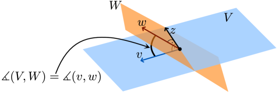
Figure 1: Computation of the angle between two planes in $\mathbbm{R}^{3}$.

By normalizing we find the bases

$$V_{B} =\begin{pmatrix}\|v\|^{-1}v&\|z\|^{-1}z\end{pmatrix},\quad W_{B}=\begin{pmatrix}\|w\|^{-1}w&\|z\|^{-1}z\end{pmatrix}$$

and $V_{B}^{\top}W_{B}=\mathrm{diag}(\frac{v^{\top}w}{\|v\|\|w\|},1)$. Hence, we obtain $\measuredangle(V,W)=\arccos(\frac{|v^{\top}w|}{\|v\|\|w\|})=\measuredangle(v,w)$.

2.2 The outer angular spectrum: definition and an elementary property

For $n\in\mathbbm{N}$ we abbreviate the average of principal angles between successive subspaces by

(4) $$\alpha_{n}:\begin{array}[]{rcl}\mathcal{G}(s,d)&\to&[0,\frac{\pi}{2}]\\[2.84526pt] V&\mapsto&\displaystyle\frac{1}{n}\sum_{j=1}^{n}\measuredangle(\Phi(j-1,0)V,\Phi(j,0)V).\end{array}$$

Definition 2.3

For $s\in\{1,\dots,d\}$ the outer angular spectrum of dimension $s$ is defined by

$$\Sigma_{s}\coloneqq\mathrm{cl}\big{\{}\theta\in[0,\tfrac{\pi}{2}]:\exists V\in\mathcal{G}(s,d):\varliminf_{n\to\infty}\alpha_{n}(V)\leq\theta\leq\varlimsup_{n\to\infty}\alpha_{n}(V)\big{\}}.$$

When we consider different systems we will write $\Sigma_{s}(\Phi)$ to indicate the dependence of the angular spectrum on the solution operator. Since we take the closure the corresponding resolvent set $[0,\frac{\pi}{2}]\setminus\Sigma_{s}$ is relatively open. Further, each value $\theta\in\Sigma_{s}$ is an accumulation point of $(\alpha_{n}(V))_{n\in\mathbbm{N}}$ for some $V\in\mathcal{G}(s,d)$.

Lemma 2.4

Let $V\in\mathcal{G}(s,d)$. Then each

$$\theta\in\big{[}\varliminf_{n\to\infty}\alpha_{n}(V),\varlimsup_{n\to\infty}\alpha_{n}(V)\big{]}$$

is an accumulation point of $(\alpha_{n}(V))_{n\in\mathbbm{N}}$.

Proof 2.5

With $a_{j}=\measuredangle(\Phi(j-1,0)V,\Phi(j,0)V)\in[0,\frac{\pi}{2}]$ we observe for $n\in\mathbbm{N}$ that

$$|\alpha_{n}(V)-\alpha_{n+1}(V)| =\left|\frac{1}{n}\sum_{j=1}^{n}a_{j}-\frac{1}{n+1}\sum_{j=1}^{n+1}a_{j}\right|=\left|\frac{1}{n^{2}+n}\sum_{j=1}^{n}a_{j}-\frac{1}{n+1}a_{n+1}\right|$$

$$\leq\frac{1}{n^{2}+n}\cdot n\cdot\frac{\pi}{2}+\frac{1}{n+1}\cdot\frac{\pi}{2}=\frac{\pi}{n+1},$$

hence $\lim_{n\to\infty}\alpha_{n}(V)-\alpha_{n+1}(V)=0$. Therefore, each value between $\varliminf_{n\to\infty}\alpha_{n}(V)$ and $\varlimsup_{n\to\infty}\alpha_{n}(V)$ is approached by a convergent subsequence of $\alpha_{n}(V)$.

2.3 Relation to angular values

Several different types of angular values have been proposed in [6]. These values have in common that the supremum over $V\in\mathcal{G}(s,d)$ is taken. For the relation to the angular spectrum defined above, it is useful to consider also the infimum w.r.t.  $V\in\mathcal{G}(s,d)$. We introduce these notions but restrict the presentation to the so called outer angular values (see [6, Section 3.1] for inner and uniform versions).

Definition 2.6

Let the nonautonomous system (1) and $s\in\{1,\ldots,d\}$ be given. The outer angular values of dimension $s$ are defined by

$$\theta_{s}^{\sup,\varlimsup}=\sup_{V\in\mathcal{G}(s,d)}\varlimsup_{n\to\infty}\alpha_{n}(V),\quad\theta_{s}^{\sup,\varliminf}=\sup_{V\in\mathcal{G}(s,d)}\varliminf_{n\to\infty}\alpha_{n}(V),$$

$$\theta_{s}^{\inf,\varlimsup}=\inf_{V\in\mathcal{G}(s,d)}\varlimsup_{n\to\infty}\alpha_{n}(V),\quad\theta_{s}^{\inf,\varliminf}=\inf_{V\in\mathcal{G}(s,d)}\varliminf_{n\to\infty}\alpha_{n}(V).$$

The following relations hold for all $s=1,\ldots,d$

(5) $$\begin{matrix}\theta_{s}^{\inf,\varliminf}&\leq&\theta_{s}^{\inf,\varlimsup}\\ \rotatebox[origin={c}]{-90.0}{$\leq$}&&\rotatebox[origin={c}]{-90.0}{$\leq$}\\ \theta_{s}^{\sup,\varliminf}&\leq&\theta_{s}^{\sup,\varlimsup}.\end{matrix}$$

For the $\sup_{V}$-values we refer to [6, Lemm 3.3] while the other relations are rather obvious. Note that these values are generally not identical; see [6, Section 3.2]. In particular, for the example in [6, 3.10] the $\sup_{V\in\mathcal{G}(1,2)}$ and $\inf_{V\in\mathcal{G}(1,2)}$ coincide and the diagram reads

$$\begin{matrix}\theta_{1}^{\inf,\varliminf}&<&\theta_{1}^{\inf,\varlimsup}\\ \rotatebox[origin={c}]{-90.0}{$=$}&&\rotatebox[origin={c}]{-90.0}{$=$}\\ \theta_{1}^{\sup,\varliminf}&<&\theta_{1}^{\sup,\varlimsup}.\end{matrix}$$

The following proposition is a consequence of the definitions.

Proposition 2.7

The outer angular spectrum of dimension $s$ satisfies

(6) $$\{\theta_{s}^{\inf,\varliminf},\theta_{s}^{\inf,\varlimsup},\theta_{s}^{\sup,\varliminf},\theta_{s}^{\sup,\varlimsup}\}\subseteq\Sigma_{s}\subseteq[\theta_{s}^{\inf,\varliminf},\theta_{s}^{\sup,\varlimsup}].$$

Proof 2.8

For any $\varepsilon>0$ there exists $V\in\mathcal{G}(s,d)$ such that $\theta_{s}^{\inf,\varliminf}\leq\varliminf_{n\to\infty}\alpha_{n}(V)\leq\theta_{s}^{\inf,\varliminf}+\varepsilon$. Since $\varliminf_{n\to\infty}\alpha_{n}(V)\in\Sigma_{s}$ holds by definition and $\Sigma_{s}$ is closed we obtain $\theta_{s}^{\inf,\varliminf}\in\Sigma_{s}$. A similar argument applies to the other angular values. The second inclusion in (6) is immediate from the definitions.

Of course, in general there is more structure to the spectrum inside the bounding interval as the following example shows.

Example 2.9

Consider (1) for the $3$-dimensional autonomous case

(7) $$A_{n}=A=\begin{pmatrix}T_{\varphi}&0\\ 0&2\end{pmatrix},\quad T_{\varphi}=\begin{pmatrix}\cos(\varphi)&-\sin(\varphi)\\ \sin(\varphi)&\cos(\varphi)\end{pmatrix},\quad n\in\mathbbm{N}_{0},\ 0<\varphi\leq\frac{\pi}{2}.$$

For $V=\mathrm{span}(v)$, $v=(z,v_{3})^{\top}\neq 0$, $z\in\mathbbm{R}^{2}$ we obtain

$$\lim_{n\to\infty}\alpha_{n}(V)=\begin{cases}0,&\text{if}\quad v_{3}\neq 0,\\ \varphi,&\text{if}\quad v_{3}=0.\end{cases}$$

This follows from

$$A^{j}v =\begin{pmatrix}T_{j\varphi}z\\ 0\end{pmatrix},\quad\measuredangle(A^{j-1}v,A^{j}v)=\varphi\quad\text{if}\quad v_{3}=0,$$

$$\measuredangle(A^{j-1}v,A^{j}v) =\measuredangle\left(\begin{pmatrix}T_{(j-1)\varphi}z\\ 2^{j-1}v_{3}\end{pmatrix},\begin{pmatrix}T_{j\varphi}z\\ 2^{j}v_{3}\end{pmatrix}\right)$$

$$=\measuredangle\left(\begin{pmatrix}2^{1-j}v_{3}^{-1}T_{(j-1)\varphi}z\\ 1\end{pmatrix},\begin{pmatrix}2^{-j}v_{3}^{-1}T_{j\varphi}z\\ 1\end{pmatrix}\right)\to 0\;\text{as}\;j\to\infty,\;\text{if}\;v_{3}\neq 0.$$

For a precise estimate in the last case see [6, Section 3.1]. Therefore, the inclusion (6) for this example reads

$$\{\theta_{1}^{\inf,\varliminf},\theta_{1}^{\sup,\varlimsup}\}=\{0,\varphi\}=\Sigma_{1}\subsetneq[0,\varphi]=[\theta_{1}^{\inf,\varliminf},\theta_{1}^{\sup,\varlimsup}].$$

A more intriguing example is the following autonomous system (1) for the orthogonal normal form of a $2\times 2$-matrix with complex conjugate eigenvalues; see [6, Sections 5.1,6.1].

Example 2.10

(8) $$A(\rho,\varphi)=\begin{pmatrix}\cos(\varphi)&-\rho^{-1}\sin(\varphi)\\ \rho\sin(\varphi)&\cos(\varphi)\end{pmatrix},\quad 0<\rho\leq 1,\quad 0<\varphi\leq\frac{\pi}{2}.$$

In [6, Proposition 5.2] we showed that all angular values agree in this case, and in [6, Theorem 6.1] we determined an explicit formula for $\theta_{1}^{\sup,\lim}(A(\rho,\varphi))$. It depends on the skewness parameter $\mathrm{sk}(\rho,\varphi)=\frac{1}{2}(\rho+\rho^{-1})\sin(\varphi)$ and on $\frac{\varphi}{\pi}$ being rational or irrational. The proof of [6, Theorem 6.1] does not only provide the maximal angular value $\theta_{1}^{\sup,\lim}(A(\rho,\varphi))$ but also the minimal one $\theta_{1}^{\inf,\lim}(A(\rho,\varphi))$ and thus the angular spectrum $\Sigma_{1}(A(\rho,\varphi))$. Therefore, we don’t repeat the computation here. The result is the following:

(9) $$\Sigma_{1}(A(\rho,\varphi))=\begin{cases}\begin{array}[]{ll}\{\varphi\},&\mathrm{sk}(\rho,\varphi)\leq 1,\\ \displaystyle\Big{\{}\varphi+\frac{1}{\pi}\int_{\{\delta_{\rho,\varphi}<0\}}\delta_{\rho,\varphi}(\theta)\mathrm{d}\theta\Big{\}},&\mathrm{sk}(\rho,\varphi)>1,\frac{\varphi}{\pi}\notin\mathbbm{Q},\\ \left[\min_{0\leq\theta\leq\frac{\pi}{2}}G_{q}(\theta),\max_{0\leq\theta\leq\frac{\pi}{2}}G_{q}(\theta)\right],&\mathrm{sk}(\rho,\varphi)>1,\frac{\varphi}{\pi}=\frac{p}{q},q\perp p.\end{array}\end{cases}$$

Here the functions $\delta_{\rho,\varphi},G_{q}:[0,\pi]\to\mathbbm{R}$ and $\Psi_{\rho}:\mathbbm{R}\to\mathbbm{R}$ are defined as follows:

(10) $$\Psi_{\rho}(\theta) =\begin{cases}\arctan(\rho\tan(\theta)),&|\theta|<\frac{\pi}{2},\\ \theta,&|\theta|=\frac{\pi}{2},\end{cases}$$

$$\Psi_{\rho}(\theta+n\pi) =\Psi_{\rho}(\theta)+n\pi,\text{ for }|\theta|\leq\frac{\pi}{2},n\in\mathbbm{Z}\setminus\{0\},$$

$$\delta_{\rho,\varphi}(\theta) =2\Psi_{\rho}(\theta)-2\Psi_{\rho}(\theta+\varphi)+\pi,$$

$$G_{q}(\theta) =\frac{1}{q}\sum_{j=1}^{q}\min(\theta_{j}-\theta_{j-1},\theta_{j-1}+\pi-\theta_{j}),\quad\theta_{j-1}=\Psi_{\rho}((j-1)\varphi+\Psi_{\rho^{-1}}(\theta)).$$

If $\frac{\pi}{2}<\varphi<\pi$ then $\Sigma_{1}(A(\rho,\varphi))=\Sigma_{1}(A(\rho,\pi-\varphi))$.

Figure 2: Outer angular spectrum of the autonomous system $u_{n+1}=A(\rho,\varphi)u_{n}$ for $A(\rho,\varphi)$ from (8) as a function of the parameters $\rho\in(0,1]$, $\varphi\in(0,\frac{\pi}{2}]$.

Figure 2 illustrates the rather irregular behavior of the outer angular spectrum with respect to the parameters $\rho$ and $\varphi$. In the hatched region $\mathrm{sk}(\rho,\varphi)\leq 1$ we always have point spectrum $\{\varphi\}$. One can show that in this region no turnover occurs, i.e. the angle between the subspaces $\mathrm{span}(v)$ and $\mathrm{span}(A(\rho,\varphi)v)$ always coincides with the angle between the spanning vectors. This changes in the region $\mathrm{sk}(\rho,\varphi)>1$. Then we find point spectrum at $\varphi$-values not in $\pi\mathbbm{Q}$ while we have perfect intervals for $\varphi$-values in $\pi\mathbbm{Q}$. In the latter case the left and right endpoint of the spectral interval are indicated in Figure 2 by a dot. Let us further note that for values $\varphi\notin\pi\mathbbm{Q}$ and $\mathrm{sk}(\rho,\varphi)>1$ the function $\delta_{\rho,\varphi}$ becomes negative in some open subinterval of $(0,\frac{\pi}{2})$, so that $\Sigma_{1}(A(\rho,\varphi))$ is strictly below $\varphi$ (cf. [6, (6.8)]). On the other hand, by [6, Theorem 6.1] we have $\max_{0\leq\theta\leq\frac{\pi}{2}}G_{q}(\theta)=\varphi$ if $\mathrm{sk}(\rho,\varphi)>1$ and $\varphi=\frac{\pi}{q}$ for some $q\in\mathbbm{N},q\geq 2$, i.e. the maximum angular value is achieved for a proper one-dimensional subspace. Finally, we showed in [9, Section 4.4], [6, Section 6.1] that the maximum value $\theta_{1}^{\sup,\lim}(A(\rho,\varphi))$ is upper but not lower semicontinuous w.r.t. the parameter $\varphi$. Similarly, one finds that $\theta_{1}^{\inf,\lim}(A(\rho,\varphi))$ is lower but not upper semicontinuous w.r.t. $\varphi$. In view of the formula (9) this shows that the angular spectrum is upper but not lower semicontinuous w.r.t. $\varphi$ in the Hausdorff sense.

2.4 Trace spaces and the reduction theorem for the angular spectrum

In [8, Section 3.1] we introduced so called trace spaces which are associated with the Grassmannian $\mathcal{G}(s,d)$ and the system (1). These are subspaces of dimension $s$ with a basis consisting of vectors from the spectral bundles of the dichotomy spectrum; see Definition 2.17 below. Trace spaces turn out to be the natural nonautonomous generalization of invariant subspaces for autonomous systems. They allow an efficient computation of outer angular values, by reducing the suprema and infima over the whole Grassmannian to the set of trace spaces, see the reduction Theorem 2.18 below.

The dichotomy spectrum, see [27] is based on the notion of an exponential dichotomy, cf. [14, 2, 18, 11, 12, 22]. We define this notion for linear systems (1) on a discrete time interval $J=\{n\in\mathbbm{Z}:n\geq n_{-}\}$ unbounded from above. For our purposes, it is convenient to use a generalized version which allows an arbitrary split of the rates of solutions, not necessarily into growing and decaying ones.

Definition 2.11

The system (1) has a generalized exponential dichotomy (GED) on $J$ with rates $0\leq\lambda_{+}<\lambda_{-}\leq\infty$ (  $(\lambda_{+},\lambda_{-})=(0,\infty)$ excluded), if there exist a constant $K>0$ and families of projectors $P_{n}^{+}$, $P_{n}^{-}\coloneqq I-P_{n}^{+}$, $n\in J$ with the properties:

• $P_{n}^{\pm}\Phi(n,m)=\Phi(n,m)P_{m}^{\pm}$ for all $n,m\in J$,

• the following estimates hold for all $n,m\in J$

  (11) $$\|\Phi(n,m)P_{m}^{+}\| \leq K\lambda_{+}^{n-m},\quad n\geq m,$$

  (12) $$\|\Phi(n,m)P_{m}^{-}\| \leq K\lambda_{-}^{n-m},\quad n\leq m.$$

The tuple $(K,\lambda_{\pm},P_{n}^{\pm})_{n\in J}$ is called the dichotomy data of (1) resp. of $\Phi$.

Remark 2.12

If $\lambda_{+}=0,\lambda_{-}<\infty$ the estimate (11) is to be read with $0^{k}=0$ for $k\geq 0$, so that $P_{m}^{+}=0$, $P_{m}^{-}=I$ follows and (12) is an upper bound for the inverse solution operator. Similarly, if $0<\lambda_{+},\lambda_{-}=\infty$ the estimate (12) is to be read with $\infty^{k}=0$ for $k\leq 0$, so that $P_{m}^{-}=0$, $P_{m}^{+}=I$ follows and (11) is an upper bound for the solution operator.

Recall that the system (1) has a (standard) exponential dichotomy (ED) (see e.g. [3, 24, 8]), if there exist constants $\alpha_{s},\alpha_{u}<1$ and projectors $P_{n}^{s},P_{n}^{u}=I-P_{n}^{s}$ which satisfy condition (i) of Definition 2.11 and

$$\|\Phi(n,m)P_{m}^{s}\|\leq K\alpha_{s}^{n-m},\quad\|\Phi(m,n)P_{n}^{u}\|\leq K\alpha_{u}^{n-m},\quad\forall\,n\geq m\in J.$$

The relation between a GED and an ED is easily established via the scaled equation

(13) $$u_{n+1}=\frac{1}{\lambda}A_{n}u_{n},\quad n\in J,\quad\lambda>0$$

which has the solution operator $\Phi_{\lambda}(n,m)=\lambda^{m-n}\Phi(n,m)$.

Lemma 2.13

If $\Phi$ has a GED with data $(K,\lambda_{\pm},P_{n}^{\pm})_{n\in J}$ then $\Phi_{\lambda}$ has an ED with data $(K,P_{n}^{s}=P_{n}^{+},P_{n}^{u}=P_{n}^{-},\alpha_{s}=\frac{\lambda_{+}}{\lambda},\alpha_{u}=\frac{\lambda}{\lambda_{-}})_{n\in J}$ for each $\lambda\in(\lambda_{+},\lambda_{-})$.
Conversely, if $\Phi_{\lambda}$ has an ED with data $(K,\alpha_{s,u},P_{n}^{s,u})_{n\in J}$ then $\Phi$ has a GED with data $(K,\lambda_{+}=\alpha_{s}\lambda,\lambda_{-}=\frac{\lambda}{\alpha_{u}},P_{n}^{+}=P_{n}^{s},P_{n}^{-}=P_{n}^{u})_{n\in J}$.

For the further development of the theory (in particular Section 3) it is suitable to use the GED setting throughout and avoid working with the scaled equation (13). As an example, we state and prove two properties of GEDs which are well-known for EDs.

Lemma 2.14

The ranges of projectors of a GED are uniquely determined by

(14) $$\mathcal{R}(P_{m}^{+})=\{x\in\mathbbm{R}^{d}:\exists C>0:\|\Phi(n,m)x\|\leq C\lambda_{+}^{n-m}\|x\|\quad\forall\;n\geq m\in J\}.$$

If $(\tilde{K},\lambda_{\pm},\tilde{P}_{n}^{\pm})_{n\in J})$ are the data of another GED with the same rates, then the following holds

(15) $$\|P_{n}^{+}-\tilde{P}_{n}^{+}\|\leq K^{2}\left(\frac{\lambda_{+}}{\lambda_{-}}\right)^{n-n_{-}}\|P_{n_{-}}^{+}-\tilde{P}_{n_{-}}^{+}\|,\quad n\in J.$$

Proof 2.15

The relation “ $\subseteq$ “ in (14) is obvious. For the converse, consider $x\in\mathbbm{R}^{d}$ with $\|\Phi(n,m)x\|\leq C\lambda_{+}^{n-m}\|x\|$ for $n\geq m$. Then we conclude from (12)

$$\|P_{m}^{-}x\|=\|P_{m}^{-}\Phi(m,n)\Phi(n,m)x\|\leq KC\left(\frac{\lambda^{+}}{\lambda^{-}}\right)^{n-m}\|x\|,\quad n\geq m.$$

The right-hand side converges to zero as $n\to\infty$, hence we obtain $P_{m}^{-}x=0$ and $x\in\mathcal{R}(P_{m}^{+})$. For the second assertion note that $\mathcal{R}(P_{n}^{+})=\mathcal{R}(\tilde{P}_{n}^{+})$ implies $P_{n}^{+}\tilde{P}_{n}^{+}=\tilde{P}_{n}^{+}$, $\tilde{P}_{n}^{+}P_{n}^{+}=P_{n}^{+}$ and, therefore,

$$P_{n}^{+}(P_{n}^{+}-\tilde{P}_{n}^{+})P_{n}^{-}=P_{n}^{+}(P_{n}^{+}-\tilde{P}_{n}^{+})(I-P_{n}^{+})=P_{n}^{+}\tilde{P}_{n}^{+}(P_{n}^{+}-I)=P_{n}^{+}-\tilde{P}_{n}^{+}.$$

The dichotomy estimates then show

$$\|P_{n}^{+}-\tilde{P}_{n}^{+}\| =\|\Phi(n,n_{-})(P_{n_{-}}^{+}-\tilde{P}_{n_{-}}^{+})\Phi(n_{-},n)\|$$

$$=\|\Phi(n,n_{-})P_{n_{-}}^{+}(P_{n_{-}}^{+}-\tilde{P}_{n_{-}}^{+})P_{n}^{-}\Phi(n_{-},n)\|$$

$$\leq K\lambda_{+}^{n-n_{-}}\|P_{n_{-}}^{+}-\tilde{P}_{n_{-}}^{+}\|K\lambda_{-}^{n_{-}-n}.$$

Next, we define the dichotomy spectrum and the resolvent set in the GED setting.

Definition 2.16

The dichotomy resolvent set and dichotomy spectrum are defined by

(16) $$R_{\mathrm{ED}} =\bigcup\{(\lambda_{+},\lambda_{-}):\eqref{diffeq}\;\text{has a GED with rates}\;\lambda_{+}<\lambda_{-}\;\text{on}\;J\}$$

$$\Sigma_{\mathrm{ED}} =(0,\infty)\setminus R_{\mathrm{ED}}.$$

Note that $R_{\mathrm{ED}}$ is open and $\Sigma_{\mathrm{ED}}$ is closed relative to $(0,\infty)$. Then we always have $(0,\varepsilon),(\varepsilon^{-1},\infty)\subseteq R_{\mathrm{ED}}$ for some $\varepsilon>0$ since the matrices $A_{n}$ and their inverses are uniformly bounded. Further, the GED and thus also the spectral notions remain unchanged when we replace $J$ by a smaller interval $\{n\in\mathbbm{Z}:n\geq N\}$ for some $N\geq n_{-}$. However, we do not set $n_{-}=0$ in general, since we will derive estimates with constants independent of $n_{-}$ and then let $n_{-}$ tend to infinity.

By Lemma 2.13, the definition (16) agrees with the usual one for spectrum and resolvent set in the ED setting ([3, 24, 8]):

$$R_{\mathrm{ED}} =\{\lambda>0:\Phi_{\lambda}\text{ has an ED on }J\},$$

$$\Sigma_{\mathrm{ED}} =\{\lambda>0:\Phi_{\lambda}\text{ has no ED on }J\}.$$

The Spectral Theorem [3, Theorem 3.4] provides the decomposition $\Sigma_{\mathrm{ED}}=\bigcup_{k=1}^{\varkappa}\mathcal{I}_{k}$ of the dichotomy spectrum into $\varkappa\leq d$ spectral intervals

$$\mathcal{I}_{k}=[\sigma_{k}^{-},\sigma_{k}^{+}],\ k=1,\dots,\varkappa,\quad\text{where}\quad 0<\sigma_{\varkappa}^{-}\leq\sigma_{\varkappa}^{+}<\dots<\sigma_{1}^{-}\leq\sigma_{1}^{+}<\infty.$$

Similarly, one decomposes the resolvent set $R_{\mathrm{ED}}=\bigcup_{k=1}^{\varkappa+1}R_{k}$ into disjoint open intervals

$$R_{k}=(\sigma_{k}^{+},\sigma_{k-1}^{-}),\ k=1,\ldots,\varkappa+1,\text{ where }\sigma_{\varkappa+1}^{+}=0,\quad\sigma_{0}^{-}=\infty,$$

see Figure 3. If $\sigma_{k}^{-}=\sigma_{k}^{+}$ holds for an index $k\in\{1,\dots,\varkappa\}$ then the spectral interval $\mathcal{I}_{k}$ degenerates into an isolated point. For every $\lambda\in R_{k}$, $k\in\{1,\dots,\varkappa+1\}$ one has dichotomy projectors $P_{n,k}^{+}$, $P_{n,k}^{-}=I-P_{n,k}^{+}$ for $n\in J$ of (13), which depend on $k$ but not on $\lambda\in R_{k}$; see Lemma 2.13. By the characterization (14) it is immediate that the ranges of the projectors form an increasing flag of subspaces, i.e.

(17) $$\{0\}=\mathcal{R}(P_{n,\varkappa+1}^{+})\subseteq\mathcal{R}(P_{n,\varkappa}^{+})\subseteq\dots\subseteq\mathcal{R}(P_{n,1}^{+})=\mathbbm{R}^{d}.$$

One can further choose the projectors such that the nullspaces, or equivalently the ranges of the complementary projectors, form a decreasing flag of subspaces:

(18) $$\mathbbm{R}^{d}=\mathcal{R}(P_{n,\varkappa+1}^{-})\supseteq\mathcal{R}(P_{n,\varkappa}^{-})\supseteq\dots\supseteq\mathcal{R}(P_{n,1}^{-})=\{0\}.$$

Given this situation, one introduces spectral bundles as follows:

(19) $$\mathcal{W}^{k}_{n} \coloneqq\mathcal{R}(P_{n,k}^{+})\cap\mathcal{R}(P_{n,k+1}^{-}),\quad k=1,\dots,\varkappa.$$

The fiber projector $\mathcal{P}_{n,k},\ k=1,\ldots,\varkappa$ onto $\mathcal{W}_{n}^{k}$ along $\bigoplus_{\nu=1,\nu\neq k}^{\varkappa}\mathcal{W}_{n}^{\nu}$ is given by

(20) $$\mathcal{P}_{n,k}=P_{n,k}^{+}P_{n,k+1}^{-}=P_{n,k+1}^{-}P_{n,k}^{+}=P_{n,k}^{+}-P_{n,k+1}^{+}=P_{n,k+1}^{-}-P_{n,k}^{-}.$$

Spectral bundles satisfy for $k=1,\dots,\varkappa$ and $n,m\in J$ the invariance condition

(21) $$\Phi(n,m)\mathcal{W}_{m}^{k}=\mathcal{W}_{n}^{k}.$$

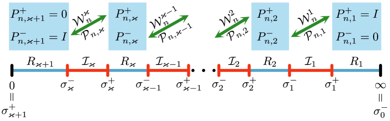
Figure 3: Illustration of spectral intervals (red), of resolvent intervals (blue) and the construction of spectral bundles with corresponding fiber projectors.

Definition 2.17

Every element $V\in\mathcal{G}(s,d)$ of the form

$$V=\bigoplus_{k=1}^{\varkappa}W_{k}:\quad W_{k}\subseteq\mathcal{W}_{n}^{k}\;\text{(subspace)}\;k=1,\ldots,\varkappa,\quad\sum_{k=1}^{\varkappa}\dim W_{k}=s$$

is called a trace space at time $n$. The set of all trace spaces at time $n$ is denoted by $\mathcal{D}_{n}(s,d)$.

The corresponding trace projectors $\mathcal{T}_{n}:\mathcal{G}(s,d)\to\mathcal{D}_{n}(s,d)$ are defined by

(22) $$\mathcal{T}_{n}(V)=\bigoplus_{k=1}^{\varkappa}(P_{n,k+1}^{-}(\mathcal{R}(P_{n,k}^{+})\cap V)).$$

From ([8, (3.18)]) we have that the trace projectors are onto, i.e.

(23) $$\mathcal{D}_{n}(s,d)=\{\mathcal{T}_{n}(V):V\in\mathcal{G}(s,d)\}.$$

Moreover, from (21), (22), (23) one infers invariance according to

(24) $$\Phi(n,m)\mathcal{T}_{m}(V)=\mathcal{T}_{n}(\Phi(n,m)V),\quad\Phi(n,m)\mathcal{D}_{m}(s,d)=\mathcal{D}_{n}(s,d).$$

Note that $\mathcal{D}_{n}(s,d)$ is usually substantially smaller than $\mathcal{G}(s,d)$ and even finite if all spectral bundles are one-dimensional [8, (3.25)]. We cite the reduction theorem [8, Theorem 3.6] on $J=\mathbbm{N}_{0}$ by using the averages from (4).

Theorem 2.18

Assume that the difference equation (1) has the dichotomy spectrum $\Sigma_{\mathrm{ED}}=\bigcup_{k=1}^{\varkappa}[\sigma_{k}^{-},\sigma_{k}^{+}]$ with fibers $\mathcal{W}_{n}^{k},\ k=1\ldots,\varkappa$ and trace projector (22). Then the following equality holds for all $V\in\mathcal{G}(s,d)$

(25) $$\varlimsup_{n\to\infty}\alpha_{n}(V)=\varlimsup_{n\to\infty}\alpha_{n}(\mathcal{T}_{0}(V)),$$

and similarly with $\varliminf$ instead of $\varlimsup$.

An immediate consequence of this theorem is the reduction of angular values and of the outer angular spectrum to the set of traces spaces.

Theorem 2.19

Under the assumption of Theorem 2.18 the outer angular values are given by

(26) $$\theta_{s}^{\sup,\varlimsup} =\sup_{V\in\mathcal{D}_{0}(s,d)}\varlimsup_{n\to\infty}\alpha_{n}(V),\quad\theta_{s}^{\sup,\varliminf}=\sup_{V\in\mathcal{D}_{0}(s,d)}\varliminf_{n\to\infty}\alpha_{n}(V),$$

$$\theta_{s}^{\inf,\varlimsup} =\inf_{V\in\mathcal{D}_{0}(s,d)}\varlimsup_{n\to\infty}\alpha_{n}(V),\quad\theta_{s}^{\inf,\varliminf}=\inf_{V\in\mathcal{D}_{0}(s,d)}\varliminf_{n\to\infty}\alpha_{n}(V),$$

and the outer angular spectrum satisfies

(27) $$\Sigma_{s}=\mathrm{cl}\big{\{}\theta\in[0,\tfrac{\pi}{2}]:\exists V\in\mathcal{D}_{0}(s,d):\varliminf_{n\to\infty}\alpha_{n}(V)\leq\theta\leq\varlimsup_{n\to\infty}\alpha_{n}(V)\big{\}}.$$

Example 2.20

(Example 2.9 revisited) Spectral bundles of the dichotomy spectrum are eigenspaces given by

$$\mathcal{W}_{0}^{1} ={\mathrm{span}}\begin{pmatrix}0&0&1\end{pmatrix}^{\top},\quad\mathcal{W}_{0}^{2}={\mathrm{span}}\left(\begin{pmatrix}1&0&0\end{pmatrix}^{\top},\begin{pmatrix}0&1&0\end{pmatrix}^{\top}\right).$$

By Theorem 2.19 it suffices to consider for $s=1$ initial spaces $V=\mathrm{span}(v)$ with either $v\in\mathcal{W}_{0}^{1}$ or $v\in\mathcal{W}_{0}^{2}$. This shows that the computation for the mixed case in Example 2.9 was not necessary. Moreover, we obtain the angular values listed in Table 1 and the angular spectrum for $s=1$ and $s=2$ as follows:

$$\Sigma_{s}=\{0,\varphi\}\subseteq[\theta_{s}^{\inf,\varliminf},\theta_{s}^{\sup,\varlimsup}]=[0,\varphi].$$

angular value	achieved in
$\theta_{1}^{\inf,\varliminf}=0$	$V=\mathcal{W}_{0}^{1}$
$\theta_{1}^{\sup,\varlimsup}=\varphi$	$V={\mathrm{span}}\begin{pmatrix}1&0&0\end{pmatrix}^{\top}$
$\theta_{2}^{\inf,\varliminf}=0$	$V=\mathcal{W}_{0}^{2}$
$\theta_{2}^{\sup,\varlimsup}=\varphi$	$V={\mathrm{span}}\left(\begin{pmatrix}0&0&1\end{pmatrix}^{\top},\begin{pmatrix}1&0&0\end{pmatrix}^{\top}\right)$

Table 1: Outer angular values for (7).

Example 2.21

As a continuation of Examples 2.10 and 2.20 we determine $\Sigma_{2}(A)$ for

(28) $$A=\begin{pmatrix}B&b\\ 0&\lambda\end{pmatrix}\in\mathbbm{R}^{3,3},\quad b\in\mathbbm{R}^{2},\ |\lambda|\neq 1,\ B=A(\rho,\varphi)\ (\text{see }\eqref{rhomatrix}).$$

Note that $\left(\begin{smallmatrix}w\\ 1\end{smallmatrix}\right)$ with $w=(\lambda I_{2}-B)^{-1}b$ is an eigenvector of $A$ with eigenvalue $\lambda$. Further, the matrix $A$ in (28) is the Schur normal form of a general real $3\times 3$-matrix which has a complex conjugate eigenvalue of modulus $1$ and a real eigenvalue of modulus $\neq 1$. The dichotomy spectrum is $\{1,|\lambda|\}$ and Theorem 2.19 shows that it suffices to study two-dimensional subspaces $V_{0}$ of $\mathbbm{R}^{3}$ which have basis vectors from $\mathbbm{R}^{2}\times\{0\}$ or $\mathrm{span}\left(\begin{smallmatrix}w\\ 1\end{smallmatrix}\right)$. If both are from the first space then the resulting angular value vanishes. Hence, we consider

$$V_{0}=\mathrm{span}\left(\begin{pmatrix}x_{0}\\ 0\end{pmatrix},\begin{pmatrix}w\\ 1\end{pmatrix}\right),\quad x_{0}\in\mathbbm{R}^{2},\ x_{0}\neq 0.$$

For the iterates we have

$$V_{j}=A^{j}V_{0}=\mathrm{span}\left(\begin{pmatrix}x_{j}\\ 0\end{pmatrix},\begin{pmatrix}w\\ 1\end{pmatrix}\right),\quad x_{j}=B^{j}x_{0}.$$

An orthogonal (but not necessarily orthonormal) basis is

$$V_{j}=\mathrm{span}\left(Qx_{j},\begin{pmatrix}w\\ 1\end{pmatrix}\right),\quad Q=\begin{pmatrix}(1+\|w\|^{2})I_{2}-ww^{\top}\\ -w^{\top}\end{pmatrix}\in\mathbbm{R}^{3,2}.$$

According to Example 2.2 the maximal principal angle between $V_{j}$ and $V_{j-1}$ is given by

(29) $$\measuredangle(V_{j},V_{j-1})=\measuredangle(Qx_{j},Qx_{j-1}).$$

Similar to [6, Section 6.1] we determine

$$\theta_{2}(\eta)=\lim_{n\to\infty}\frac{1}{n}\sum_{j=1}^{n}\measuredangle(V_{j},V_{j-1}),\quad x_{0}=r(\eta)\coloneqq\begin{pmatrix}\cos(\eta)\\ \sin(\eta)\end{pmatrix},\quad\eta\in[0,2\pi)$$

by applying ergodic theory to the function

(30) $$g(\eta)=\measuredangle\big{(}Qr(T_{\rho,\varphi}\eta),Qr(\eta)\big{)},\quad T_{\rho,\varphi}\eta=\Psi_{\rho}\big{(}\varphi+\Psi_{\rho}^{-1}(\eta)\big{)},$$

where $\Psi_{\rho}$ is defined in (10). The result is

(31) $$\theta_{2}(\eta)=\begin{cases}\frac{1}{2\pi}\int_{0}^{2\pi}g(\Psi_{\rho}(\xi))d\xi,&\frac{\varphi}{\pi}\notin\mathbbm{Q},\\ \frac{1}{q}\sum_{\ell=0}^{q-1}g(T_{\rho,\varphi}^{\ell}\eta),&\frac{\varphi}{\pi}=\frac{p}{q},p\perp q,p,q\in\mathbbm{N}.\end{cases}$$

The second outer angular spectrum is then of the form

(32) $$\Sigma_{2}(A)=\begin{cases}\{0,\theta_{2}\},\theta_{2}\equiv\theta_{2}(\eta),&\frac{\varphi}{\pi}\notin\mathbbm{Q},\\ \{0\}\cup[\min_{\eta}\theta_{2}(\eta),\max_{\eta}\theta_{2}(\eta)],&\frac{\varphi}{\pi}\in\mathbbm{Q},\end{cases}$$

where $\theta_{2}(\eta)$ is given by (30), (31).

We numerically compute the second outer angular spectrum for the non-resonant case $\varphi=1.25$ as well as for the resonant case $\varphi=\frac{2}{5}\pi\approx 1.2566$ nearby. In particular, we illustrate in Figures 5 and 4 the influence of $\rho\in(0,1]$ and of the angle between the eigenvector $\left(\begin{smallmatrix}w\\ 1\end{smallmatrix}\right)$ and the $xy$-plane $X\coloneqq{\mathrm{span}}\left(\left(\begin{smallmatrix}1\\ 0\\ 0\end{smallmatrix}\right),\left(\begin{smallmatrix}0\\ 1\\ 0\end{smallmatrix}\right)\right)$. This angle is given by

$$\measuredangle\left(X,\begin{pmatrix}w\\ 1\end{pmatrix}\right)=:\gamma_{w}\quad\text{where}\quad\cos(\gamma_{w})=\frac{\|w\|}{\sqrt{\|w\|^{2}+1}}.$$

We choose $\gamma_{w}\in(0,\frac{\pi}{2}]$ and $w=\frac{\cos(\gamma_{w})}{\sqrt{1+\cos(\gamma_{w})^{2}}}\left(\begin{smallmatrix}1\\ 0\end{smallmatrix}\right)$ in Figures 4 and 5.

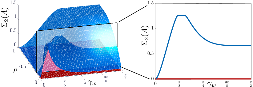
Figure 4: Computation of the second angular spectrum for the non-resonant case $\varphi=1.25$. Left panel: For each $(\gamma_{w},\rho)$-pair we obtain point spectrum only (red plane at $0$ and blue surface). Right panel: Point spectrum for fixed $\rho=0.2$.

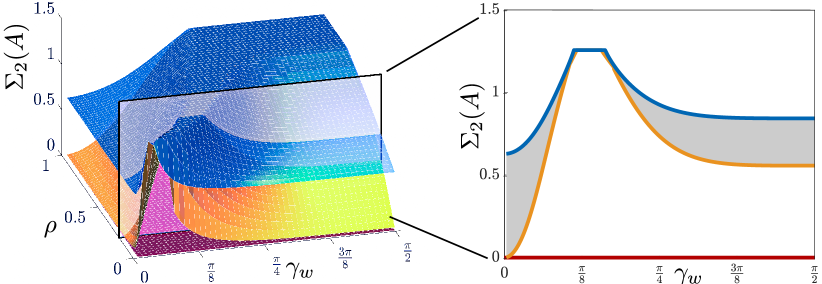
Figure 5: Computation of the second angular spectrum for the resonant case $\varphi=\frac{2}{5}\pi$. Left panel: For each $(\gamma_{w},\rho)$-pair the spectrum consists of the point spectrum $0$ (red plane) and of the interval between the orange and the blue surface. Note that in certain areas, both surfaces coincide and the spectral intervals degenerate to a point. In the intersection of this figure with the plane at $\rho=0.2$ (right panel) the spectrum consists of the curves and the grey area between them.

3 Perturbation theory and invariance of the outer angular spectrum

In this section we present some of the main theoretical results of the paper. We first show that two dynamical systems have the same outer angular spectrum if they are kinematically similar by a transformation which becomes orthogonal at infinity. In the second step we consider dynamical systems which have a rather strict dichotomy structure called complete exponential dichotomy (CED). This notion may be considered as a generalization of an autonomous system with a matrix having only semi-simple eigenvalues. Such systems do not only have a dichotomy point spectrum which is invariant under $\ell^{1}$-perturbations (a property that holds more generally [24]), but also their outer angular spectra persist under these perturbations.

3.1 Kinematic similarity and invariance

Consider a system which is kinematically similar to (1), i.e. we transform variables by $v_{n}=Q_{n}u_{n}$ with $Q_{n}\in\mathrm{GL}(\mathbbm{R}^{d})$ to obtain

(33) $$v_{n+1}=\tilde{A}_{n}v_{n},\quad\tilde{A}_{n}=Q_{n+1}A_{n}Q_{n}^{-1},\quad n\in J.$$

The corresponding solution operators $\tilde{\Phi}(n,m)$ and $\Phi(n,m)$ are related by

(34) $$\tilde{\Phi}(n,m)Q_{m}=Q_{n}\Phi(n,m),\quad n,m\in J.$$

We show that the outer angular spectrum is invariant under two types of similarity transformation.

Proposition 3.1

(Invariance of angular spectrum) The outer angular spectrum of the systems (1) and (33) coincide in the following two cases:

• $Q_{n}=q_{n}I_{d}$ holds with $q_{n}\neq 0$ for all $n\in\mathbbm{N}_{0}$.

• The limit $\lim_{n\to\infty}Q_{n}=Q\in\mathbbm{R}^{d,d}$ exists and is orthogonal.

Proof 3.2

(i): From (34) we have $\tilde{\Phi}(n,0)=\frac{q_{n}}{q_{0}}\Phi(n,0)$, hence $\tilde{\Phi}(n,0)V$ and $\Phi(n,0)V$ agree and the assertion follows from Definition 2.3.

(ii): In [9, Proposition 4.3] we have shown that for any $\varepsilon>0$ there exists $N=N(\varepsilon)$ such that for all $n\geq N$ and for all $V\in\mathcal{G}(s,d)$

(35) $$\frac{1}{n}\sum_{j=1}^{n}|\measuredangle(\tilde{\Phi}(j-1,0)Q_{0}V,\tilde{\Phi}(j,0)Q_{0}V)-\measuredangle(\Phi(j-1,0)V,\Phi(j,0)V)|\leq\varepsilon.$$

From this estimate we infer that the averages

$$\tilde{\alpha}_{n}(V)=\frac{1}{n}\sum_{j=1}^{n}\measuredangle(\tilde{\Phi}(j-1,0)V,\tilde{\Phi}(j,0)V),\quad V\in\mathcal{G}(s,d)$$

satisfy

$$\varlimsup_{n\to\infty}\tilde{\alpha}_{n}(Q_{0}V)=\varlimsup_{n\to\infty}\alpha_{n}(V),\quad\varliminf_{n\to\infty}\tilde{\alpha}_{n}(Q_{0}V)=\varliminf_{n\to\infty}\alpha_{n}(V).$$

Hence the equality of the outer angular spectra and the outer angular values follows.

3.2 Complete exponential dichotomy (CED) and persistence of angular spectrum

The following definition will be essential for the subsequent perturbation theory.

Definition 3.3

The system (1) has a complete exponential dichotomy (CED) if there exist nontrivial projectors $\mathcal{P}_{n,k}$, $n\in J$, $k=1,\ldots,\varkappa$ and constants $K>0$ and $0<\sigma_{\varkappa}<\dots<\sigma_{1}<\infty$ such that the following properties hold for all $n,m\in J$ and $k,\ell=1,\ldots,\varkappa$:

(36) $$\mathcal{P}_{n,k}\mathcal{P}_{n,\ell} =\delta_{k\ell}\mathcal{P}_{n,k},\quad\sum_{j=1}^{\varkappa}\mathcal{P}_{n,j}=I,$$

(37) $$\Phi(n,m)\mathcal{P}_{m,k} =\mathcal{P}_{n,k}\Phi(n,m),$$

(38) $$\|\Phi(n,m)\mathcal{P}_{m,k}\| \leq K\sigma_{k}^{n-m}.$$

Note that there is no restriction $n\geq m$ in the estimate (38). As usual, we denote by $(K,\sigma_{k},\mathcal{P}_{n,k})_{n\in J}^{k=1,\ldots,\varkappa}$ the dichotomy data of the CED.

Proposition 3.4

If the system (1) has a CED with data $(K,\sigma_{k},\mathcal{P}_{n,k})_{n\in J}^{k=1,\ldots,\varkappa}$ then the following estimates hold:

(39) $$\frac{1}{K}\sigma_{k}^{n-m}\|x\|\leq\|\Phi(n,m)x\|\leq K\sigma_{k}^{n-m}\|x\|\quad\forall x\in\mathcal{R}(\mathcal{P}_{m,k}),\ n,m\in J,\ k=1,\ldots,\varkappa.$$

Proof 3.5

For $x=\mathcal{P}_{m,k}x$ the estimate (38) implies the upper estimate in (39) and also the lower one as follows:

$$\|x\| =\|\mathcal{P}_{m,k}x\|=\|\Phi(m,n)\Phi(n,m)\mathcal{P}_{m,k}x\|\leq\|\Phi(m,n)\mathcal{P}_{n,k}\|\|\Phi(n,m)x\|$$

$$\leq K\sigma_{k}^{m-n}\|\Phi(n,m)x\|.$$

By this proposition the elements of $\mathcal{R}(\mathcal{P}_{m,k})$ evolve at the exact rate $\sigma_{k}$ and the rates are uniquely determined. In fact, they form the dichotomy spectrum; see Theorem 3.7 below. Nevertheless, the projectors need not be unique, as the following example shows.

Example 3.6

Consider the autonomous system $u_{n+1}=Au_{n}$ with

$$A=\mathrm{diag}(\sigma_{1},\sigma_{2},\sigma_{3})\in\mathbbm{R}^{3},\quad 0<\sigma_{3}<\sigma_{2}=1<\sigma_{1}.$$

Obviously, the system has a CED with $\varkappa=3$ and projectors $\mathcal{P}_{n,k}=e^{k}(e^{k})^{\top}$, $k=1,2,3$. However, we can also set

$$\tilde{\mathcal{P}}_{0,3} =e^{3}(e^{3}-e^{2})^{\top},\quad\tilde{\mathcal{P}}_{n,3}=A^{n}\tilde{\mathcal{P}}_{0,3}A^{-n}=e^{3}(e^{3}-\sigma_{3}^{n}e^{2})^{\top},$$

$$\tilde{\mathcal{P}}_{0,2} =(e^{3}+e^{2})(e^{2})^{\top},\quad\tilde{\mathcal{P}}_{n,2}=A^{n}\tilde{\mathcal{P}}_{0,2}A^{-n}=(\sigma_{3}^{n}e^{3}+e^{2})(e^{2})^{\top},$$

$$\tilde{\mathcal{P}}_{n,1} =P_{n,1}.$$

Since we have $\|uv^{\top}\|=\|u\|\|v\|$ for the spectral norm of a rank $1$ matrix we find for $n,m\in\mathbbm{N}_{0}$

$$\|A^{n-m}\tilde{\mathcal{P}}_{m,3}\| =\|(\sigma_{3}^{n-m}e^{3})(e^{3}-\sigma_{3}^{m}e^{2})^{\top}\|=\sigma_{3}^{n-m}\sqrt{1+\sigma_{3}^{2m}}\leq\sqrt{2}\sigma_{3}^{n-m},$$

$$\|A^{n-m}\tilde{\mathcal{P}}_{m,2}\| =\|(\sigma_{3}^{n}e^{3}+e^{2})(e^{2})^{\top}\|=\sqrt{1+\sigma_{3}^{2n}}\leq\sqrt{2}=\sqrt{2}\sigma_{2}^{n-m},$$

$$\|A^{n-m}\tilde{\mathcal{P}}_{m,1}\| =\sigma_{1}^{n-m}.$$

Thus the system also has a CED with data $(\sqrt{2},\sigma_{k},\tilde{\mathcal{P}}_{n}^{k})_{n\in\mathbbm{N}_{0}}^{k=1,2,3}$.

In the following we consider a perturbed system

(40) $$v_{n+1}=\tilde{A}_{n}v_{n},\quad\tilde{A}_{n}=A_{n}+E_{n},\quad n\in J$$

with solution operator $\tilde{\Phi}$ and state our main result.

Theorem 3.7

Let the system (1) have a CED with data $(K,\sigma_{k},\mathcal{P}_{n,k})_{n\in J}^{k=1,\ldots,\varkappa}$ and let the perturbations $E_{J}=(E_{n})_{n\in J}$ be such that $A_{n}+E_{n}$ is invertible for all $n\in J$ and

(41) $$\|E_{J}\|_{\ell^{1}}=\sum_{n\in J}\|E_{n}\|<\infty.$$

Then the perturbed system (40) has a CED with data $(\tilde{K},\sigma_{k},\tilde{\mathcal{P}}_{n,k})_{n\in J}^{k=1,\ldots,\varkappa}$ and there exists a constant $C>0$ such that

(42) $$\sup_{n\in J}\|\mathcal{P}_{n,k}-\tilde{\mathcal{P}}_{n,k}\|\leq C\sum_{n\in J}\|E_{n}\|,\quad\lim_{n\to\infty}\mathcal{P}_{n,k}-\tilde{\mathcal{P}}_{n,k}=0,\quad k=1,\ldots,\varkappa.$$

Moreover, both systems have the same dichotomy spectrum and the same outer angular spectrum

(43) $$\Sigma_{\mathrm{ED}}(\Phi)=\{\sigma_{1},\ldots,\sigma_{\varkappa}\}=\Sigma_{\mathrm{ED}}(\tilde{\Phi}),\quad\Sigma_{s}(\Phi)=\Sigma_{s}(\tilde{\Phi}).$$

Remark 3.8

From (41) and the uniform invertibility of $A_{n}$ we conclude that $A_{n}+E_{n}$ is uniformly invertible for $n$ sufficiently large. Therefore, it suffices to assume invertibility of $A_{n}+E_{n}$ for finitely many $n\in J$. Likewise, one may shrink $J$ to $\{n\in\mathbbm{Z}:n\geq N\}$ so that this assumption is not needed at all.

The proof of this theorem will take several steps in this and the next section. The final goal is to show that the system (40) is kinematically similar to the original one (1) so that Proposition 3.1 applies.

Before proceeding we consider the autonomous case.

Example 3.9

In the autonomous case $A_{n}\equiv A$ the system (1) has a CED if $A$ is invertible and (complex) diagonalizable. To see this, transform $A$ into real block-diagonal form where each block collects eigenvalues of the same absolute value, i.e.

(44) $$S^{-1}AS =\mathrm{diag}(A_{1},\ldots,A_{\varkappa}),\;A_{k}\in\mathbbm{R}^{d_{k},d_{k}},$$

$$A_{k} =\sigma_{k}\mathrm{diag}(T_{\varphi_{1}},\ldots,T_{\varphi_{\ell_{k}}},s_{1},\ldots,s_{d_{k}-2\ell_{k}}),$$

where $T_{\varphi}$ is the rotation matrix from (7) and $s_{j}\in\{-1,1\}$. For the spectral norm $\|\cdot\|_{2}$ we obtain $\|A_{k}\|_{2}^{\nu}=\sigma_{k}^{\nu}$ for all $\nu\in\mathbbm{Z}$. Further the projectors are given for $k=1,\ldots,\varkappa$, $n\in\mathbbm{N}_{0}$ by $\mathcal{P}_{n,k}=S\mathrm{diag}(0,\ldots,0,I_{d_{k}},0,\ldots,0)S^{-1}$, and they commute with $A$. Finally, the norm is defined by

$$\|x\|_{S}^{2}=\sum_{k=1}^{\varkappa}\|\mathrm{diag}(0,\ldots,0,I_{d_{k}},0,\ldots,0)S^{-1}x\|_{2}^{2},\quad x\in\mathbbm{R}^{d}.$$

A computation shows that $\|A^{\nu}\mathcal{P}_{n,k}x\|_{S}=\sigma_{k}^{\nu}\|x\|_{S}$ holds for all $x$ and $\nu\in\mathbbm{Z}$ so that conditions (36)-(38) are satisfied. Conversely, let $A$ have an eigenvalue $\lambda_{k}\in\mathbbm{C}$ of absolute value $\sigma_{k}=|\lambda_{k}|$ which is not semi-simple. Then there exists a vector $x\in\mathbbm{R}^{d}$ with $\|A^{n}x\|\asymp n\sigma_{k}^{n}\|x\|$ which violates the rate estimate (39). Hence the semi-simplicity of eigenvalues is also a necessary condition for a CED to hold.

Remark 3.10

According to Theorem 3.7, a CED implies pure point spectrum. However, the converse is not necessarily true as shown by Example 3.9. Therefore, the CED is rather a generalization of semi-simple eigenvalues than of an isolated spectrum to nonautonomous linear dynamical systems.

The following proposition relates the GED and the CED notion to each other.

Proposition 3.11

Let the system (1) and $\sigma_{\varkappa+1}=0<\sigma_{\varkappa}<\cdots<\sigma_{1}<\sigma_{0}=\infty$ be given. Then the following holds.

• If the system (1) has a CED with data $(K,\sigma_{k},\mathcal{P}_{n,k})_{n\in J}^{k=1,\ldots,\varkappa}$ then it has a GED with data $(\varkappa K,\sigma_{k+1},\sigma_{k},P_{n,k}^{+}=\sum_{\ell=k+1}^{\varkappa}\mathcal{P}_{n,\ell},P_{n,k}^{-}=\sum_{\ell=1}^{k}\mathcal{P}_{n,\ell})_{n\in J}$ for each $k=0,\ldots,\varkappa$.

• If the system (1) has a GED with data $(K,\sigma_{k+1},\sigma_{k},P_{n,k}^{+},P_{n,k}^{-})_{n\in J}$ for $k=0,\ldots,\varkappa$ then it has a CED with data $(K^{\varkappa+1},\sigma_{k},\mathcal{P}_{n,k})_{n\in J}^{k=1,\ldots,\varkappa}$ where for $n\in J$

  (45) $$\mathcal{P}_{n,k}=P_{n,k}^{-}P_{n,k-1}^{+}\cdots P_{n,0}^{+}=(I-P_{n,k}^{+})P_{n,k-1}^{+}\cdots P_{n,0}^{+},\quad k=1,\ldots,\varkappa.$$

Remark 3.12

In assertion (i) we set $\sum_{\emptyset}=0$ so that we have projectors $P_{n,\varkappa}^{+}=0$ and $P_{n,0}^{-}=0$. Similarly, note that $P_{n,0}^{+}=I$ and $P_{n,\varkappa}^{-}=I$ are used in (45).

Proof 3.13

(i)
Because of the relations (36)- (38) the matrices $P_{n,k}^{+}=\sum_{\ell=k+1}^{\varkappa}\mathcal{P}_{n,\ell}$ and $P_{n,k}^{-}=\sum_{\ell=1}^{k}\mathcal{P}_{n,\ell}$ satisfy the invariance condition (i) in Definition 2.11 and moreover

$$\|\Phi(n,m)P_{m,k}^{+}\| \leq\sum_{\ell=k+1}^{\varkappa}\|\Phi(n,m)\mathcal{P}_{m,\ell}\|\leq K\sum_{\ell=k+1}^{\varkappa}\sigma_{\ell}^{n-m}\leq(\varkappa-k)K\sigma_{k+1}^{n-m},\quad n\geq m,$$

$$\|\Phi(n,m)P_{m,k}^{-}\| \leq\sum_{\ell=1}^{k}\|\Phi(n,m)\mathcal{P}_{m,\ell}\|\leq K\sum_{\ell=1}^{k}\sigma_{\ell}^{n-m}\leq kK\sigma_{k}^{n-m},\quad n<m.$$

(ii)
From the ordering $\sigma_{k+1}<\sigma_{k}$ and the characterization (14) we obtain

(46) $$\mathcal{R}(P_{m,k}^{+})\subseteq\mathcal{R}(P_{m,\ell}^{+})\text{ , equivalently, }\quad P_{m,\ell}^{+}P_{m,k}^{+}=P_{m,k}^{+}\;\text{for}\;\ell\leq k,$$

i.e. projectors with a larger index annihilate those with smaller index from the right. We verify the properties (36)-(38) for the operators $\mathcal{P}_{n}^{k}$ from (45):

$$\sum_{k=1}^{\varkappa}\mathcal{P}_{m,k} =\sum_{k=1}^{\varkappa}P_{m,k-1}^{+}\cdots P_{m,0}^{+}-\sum_{k=1}^{\varkappa}P_{m,k}^{+}\cdots P_{m,0}^{+}$$

$$=P_{m,0}^{+}-P_{m,\varkappa}^{+}\cdots P_{m,0}^{+}=I-0=I.$$

Further, we have $\Phi(n,m)\mathcal{P}_{m,k}=\mathcal{P}_{n,k}\Phi(n,m)$ since all factors in the definition (45) have this property. Now we use (46) to show the orthogonality relations (36). For $k>\ell$ we find with $P_{m,\ell}^{-}=I-P_{m,\ell}^{+}$

$$\mathcal{P}_{m,k}\mathcal{P}_{m,\ell} =P_{m,k}^{-}P_{m,k-1}^{+}\cdots P_{m,0}^{+}P_{m,\ell-1}^{+}\cdots P_{m,0}^{+}-P_{m,k}^{-}P_{m,k-1}^{+}\cdots P_{m,0}^{+}P_{m,\ell}^{+}\cdots P_{m,0}^{+}$$

$$=P_{m,k}^{-}P_{m,k-1}^{+}\cdots P_{m,\ell}^{+}P_{m,\ell-1}^{+}\cdots P_{m,0}^{+}-P_{m,k}^{-}P_{m,k-1}^{+}\cdots P_{m,\ell}^{+}\cdots P_{m,0}^{+}=0.$$

For $k=\ell$ the first term reproduces $\mathcal{P}_{m,k}$ while the second term vanishes

$$\mathcal{P}_{m,k}\mathcal{P}_{m,k} =P_{m,k}^{-}P_{m,k-1}^{+}\cdots P_{m,0}^{+}P_{m,k-1}^{+}\cdots P_{m,0}^{+}-P_{m,k}^{-}P_{m,k-1}^{+}\cdots P_{m,0}^{+}P_{m,k}^{+}\cdots P_{m,0}^{+}$$

$$=P_{m,k}^{-}P_{m,k-1}^{+}\cdots P_{m,0}^{+}-P_{m,k}^{-}P_{m,k}^{+}\cdots P_{m,0}^{+}=\mathcal{P}_{m,k}.$$

For $k<\ell$ both terms vanish due to $P_{m,k}^{-}P_{m,j}^{+}=0$ for $j=\ell-1,\ell$:

$$\mathcal{P}_{m,k}\mathcal{P}_{m,\ell} =P_{m,k}^{-}P_{m,k-1}^{+}\cdots P_{m,0}^{+}P_{m,\ell-1}^{+}\cdots P_{m,0}^{+}-P_{m,k}^{-}P_{m,k-1}^{+}\cdots P_{m,0}^{+}P_{m,\ell}^{+}\cdots P_{m,0}^{+}$$

$$=P_{m,k}^{-}P_{m,\ell-1}^{+}\cdots P_{m,0}^{+}-P_{m,k}^{-}P_{m,\ell}^{+}\cdots P_{m,0}^{+}=0-0.$$

Finally, we use the bounds $\|P_{m,k}^{+}\|,\|P_{m,k}^{-}\|\leq K$ of projectors and the dichotomy estimates

$$\|\Phi(n,m)\mathcal{P}_{m,k}\| =\|P_{n,k}^{-}\Phi(n,m)P_{m,k-1}^{+}\cdots P_{m,0}^{+}\|\leq K^{2}\sigma_{k}^{n-m}\|P_{m,k-2}^{+}\cdots P_{m,0}^{+}\|$$

$$\leq K^{k+1}\sigma_{k}^{n-m}\quad\text{for}\quad n\geq m,$$

$$\|\Phi(n,m)\mathcal{P}_{m,k}\| =\|\Phi(n,m)P_{m,k}^{-}P_{m,k-1}^{+}P_{m}^{k,1}\cdots P_{m,0}^{+}\|\leq K\sigma_{k}^{n-m}\|P_{m,k-1}^{+}\cdots P_{m,0}^{+}\|$$

$$\leq K^{k+1}\sigma_{k}^{n-m}\quad\text{for}\quad n<m.$$

Remark 3.14

Note that the construction (45) of the fiber projectors as a product is more involved than (20) since only the first flag (17) holds automatically by (46) but not necessarily the second one (18).

Proof of Theorem 3.7 (Step 1): The system (1) has pure point dichotomy spectrum $\Sigma_{\mathrm{ED}}=\{\sigma_{1},\ldots,\sigma_{\varkappa}\}$ with associated fiber bundle $\mathcal{W}_{n}^{k}=\mathcal{R}(\mathcal{P}_{n}^{k})$, $k=1,\ldots,\varkappa$. By Proposition 3.11(i) the intervals $(\sigma_{k+1},\sigma_{k})$, $k=0,\ldots,\varkappa$ belong to the resolvent set $R_{\mathrm{ED}}$ in (16). Hence we have $\Sigma_{\mathrm{ED}}\subseteq\{\sigma_{1},\ldots,\sigma_{\varkappa}\}$. In fact, each value $\sigma_{k}$ belongs to the spectrum since the projectors $\mathcal{P}_{n,k}$ are nontrivial and the rate estimate (39) shows that $\sigma_{k}$ cannot lie in the interior of a GED interval.

3.3 Perturbation theory for CEDs

Results on perturbations of an exponential dichotomy have a long tradition, beginning with the classical roughness theorems by Coppel [11, Lecture 4] for ODEs. If the perturbations are small in $L^{\infty}$ then one obtains an exponential dichotomy with slightly weaker exponents (resp. rates) while $L^{1}$ perturbations allow to keep the exponents (resp. rates) for the perturbed system [11, Propositions 1 & 2]. The roughness theorem below transfers this principle to GEDs for systems in discrete time. From this a roughness theorem for CEDs will then follow via Proposition 3.11. Several roughness theorems for EDs in discrete time and even in noninvertible systems are well-known in the literature; see e.g. [2],[14, Theorem 7.6.7], [7, 24, 26, 25]. However, they all vary in one detail or another from the version with $\ell^{1}$-perturbations below. For example, preservation of the spectrum follows under the weaker condition of an $\ell^{0}$-perturbation [24, Cor. 3.26], while we need preservation of rates and convergence of projectors at infinity in the resolvent set. For completeness we therefore provide a proof in Appendix II.

Theorem 3.15 (Roughness of a GED)

Assume that the system (1) has a GED on $J=\{n\in\mathbbm{Z}:n\geq n_{-}\}$ with data $(K,\lambda_{\pm},P_{n}^{\pm})_{n\in J}$. Let $E_{n}\in\mathbbm{R}^{d,d}$, $n\in J$ be perturbations satisfying

(47) $$q \coloneqq K\lambda_{\star}\|E\|_{\ell^{1}(J)}<1,\text{ where}$$

$$\|E\|_{\ell^{1}(J)} =\sum_{n\in J}\|E_{n}\|,\quad\lambda_{\star}=\begin{cases}\lambda_{+}^{-1},&0<\lambda_{+}<\lambda_{-}\leq\infty,\\ \lambda_{-}^{-1},&0=\lambda_{+}<\lambda_{-}<\infty.\end{cases}$$

Then the perturbed equation (40) has a GED on $J$ with data $(\tilde{K},\lambda_{\pm},\tilde{P}_{n}^{\pm})_{n\in J}$, where

(48) $$\sup_{n\in J}\|P_{n}^{\pm}-\tilde{P}_{n}^{\pm}\|\leq\frac{qK}{1-q},\quad\tilde{K}=\frac{K}{1-q}.$$

The following corollary holds for bounded rather than small $\ell^{1}$-perturbations.

Corollary 3.16

Let the system (1) have a GED on $J$ with data $(K,\lambda_{\pm},P_{n}^{\pm})_{n\in J}$. Further assume that the perturbation satisfies $\|E_{J}\|_{\ell^{1}(J)}=\sum_{n\in J}\|E_{n}\|<\infty$, and let $A_{n}+E_{n}$ be invertible for all $n\in\mathbbm{N}_{0}$. Then there exist constants $\tilde{K},C>0$ such that the perturbed system (40) has a GED on $\mathbbm{N}_{0}$ with data $(\tilde{K},\lambda_{\pm},\tilde{P}_{n}^{\pm})_{n\in J}$. The perturbed projectors satisfy

(49) $$\sup_{n\in J}\|P_{n}^{\pm}-\tilde{P}_{n}^{\pm}\|\leq C\sum_{n\in J}\|E_{n}\|,\quad P_{n}^{\pm}-\tilde{P}_{n}^{\pm}\to 0\text{ as }n\to\infty.$$

Proof 3.17

Since $\|E_{J}\|_{\ell^{1}(J)}<\infty$ there exists $n_{+}\in J$ such that $q_{+}=K\lambda_{\star}\|E_{J_{+}}\|_{\ell^{1}(J_{+})}<1$. Then Theorem 3.15 applies to (40) on $J_{+}=\{n\in\mathbbm{N}:n\geq n_{+}\}$ and we obtain a GED on $J_{+}$ with data $(K_{+},\lambda_{\pm},\tilde{P}_{n}^{\pm})_{n\in J_{+}}$ which satisfies the estimate

(50) $$\sup_{n\in J_{+}}\|P_{n}^{\pm}-\tilde{P}_{n}^{\pm}\|\leq C_{+}\sum_{n\in J_{+}}\|E_{n}\|,\quad C_{+}=\frac{K\lambda_{\star}}{1-q_{+}}.$$

Then we extend the GED over a finite distance from $J_{+}$ to $J$ in a standard way by setting $\tilde{P}_{n}^{+}=\tilde{\Phi}(n,n_{+})\tilde{P}_{n_{+}}\tilde{\Phi}(n_{+},n)$ and by adapting the constant $K_{+}$ to some $\tilde{K}$. This yields a GED on $J$ with data $(\tilde{K},\lambda_{\pm},\tilde{P}_{n}^{\pm})_{n\in J}$. The estimate (49) on $J$ follows from (50) since the difference

$$\tilde{P}_{n}^{+}-P_{n}^{+}=\tilde{\Phi}(n,n_{+})\tilde{P}_{n_{+}}^{+}\tilde{\Phi}(n_{+},n)-\Phi(n,n_{+})P_{n^{+}}^{+}\Phi(n_{+},n),\quad n_{-}\leq n<n_{+}$$

can be bounded in terms of $\|E_{n}\|$, $n=n_{-},\ldots,n_{+}$ and $\|\tilde{P}_{n_{+}}^{+}-P_{n_{+}}^{+}\|$.

It remains to show $P_{n}^{\pm}-\tilde{P}_{n}^{\pm}\to 0$ as $n\to\infty$. For that purpose let us apply Theorem 3.15 again for arbitrary $N\geq n_{+}$ to $J_{N}=\{n\in J:n\geq N\}$ with $q_{N}=K\lambda_{\star}\|E_{J_{N}}\|_{\ell_{1}(J_{N})}\leq q_{+}<1$. Then we we find another GED of (40) with data $(K_{N},\lambda_{\pm},P(N)_{n}^{\pm})_{n\in J_{N}}$ where the constant $K_{N}=\frac{K}{1-q_{N}}\leq\frac{K}{1-q_{+}}$ is uniformly bounded w.r.t. $N$ and the estimate

$$\sup_{n\geq N}\|P_{n}^{+}-P(N)_{n}^{+}\|\leq\frac{K^{2}\lambda_{\star}}{1-q_{+}}\sum_{n\geq N}\|E_{n}\|$$

holds. Now recall that (15) implies

$$\|\tilde{P}_{n}^{+}-P(N)_{n}^{+}\|\leq\tilde{K}^{2}\left(\frac{\lambda_{+}}{\lambda_{-}}\right)^{n-N}\|\tilde{P}_{N}^{+}-P(N)_{N}^{+}\|,\quad n\geq N.$$

By the triangle inequality we have for $n\geq N$

$$\|P_{n}^{+}-\tilde{P}_{n}^{+}\|\leq\frac{K^{2}\lambda_{\star}}{1-q_{+}}\sum_{j\geq N}\|E_{j}\|+\tilde{K}^{2}\left(\frac{\lambda_{+}}{\lambda_{-}}\right)^{n-N}\|\tilde{P}_{N}^{+}-P(N)_{N}^{+}\|.$$

For a given $\varepsilon>0$ take $N=N_{1}$ so large that the first term is below $\frac{\varepsilon}{2}$ and then $n\geq N_{1}$ so large that the second term is below $\frac{\varepsilon}{2}$. This finishes the proof.

Theorem 3.18 (Roughness of a CED)

Assume that the difference equation (1) has a CED with data $(K,\sigma_{k},\mathcal{P}_{n}^{k})_{n\in J}^{k=1,\ldots,\varkappa}$ on a one-sided interval $J=\{n\in\mathbbm{Z}:n\geq n_{-}\}$. Let $(E_{n})_{n\in J}$ be a perturbation such that $A_{n}+E_{n}$ is invertible for all $n\in J$ and such that $\|E\|_{\ell^{1}}<\infty$. Then there exist constants $\tilde{K},C>0$ such that the perturbed system (40) has a CED with data $(\tilde{K},\sigma_{k},\tilde{\mathcal{P}}_{n,k})_{n\in J}^{k=1,\ldots,\varkappa}$ and such that for all $k=1,\ldots,\varkappa$

(51) $$\sup_{n\in J}\|\mathcal{P}_{n,k}-\tilde{\mathcal{P}}_{n,k}\| \leq C\sum_{\ell\in J}\|E_{\ell}\|,\quad\lim_{n\to\infty}\mathcal{P}_{n,k}-\tilde{\mathcal{P}}_{n,k}=0.$$

Proof 3.19

By Proposition 3.11(i), system (1) has GEDs with data $(K,\sigma_{k+1},\sigma_{k},P_{n,k}^{\pm})_{n\in J}$ where $P_{n,k}^{+}=\sum_{\ell=k+1}^{\varkappa}\mathcal{P}_{n,\ell}$, $P_{n,k}^{-}=I-P_{n,k}^{+}=\sum_{\ell=1}^{k}\mathcal{P}_{n}^{\ell}$ for $k=0,\ldots,\varkappa$ and $\sigma_{0}=0$, $\sigma_{\varkappa+1}=\infty$. The Roughness Theorem 3.15 for GEDs and Corollary 3.16 ensure that the perturbed system (40) has GEDs with data $(\tilde{K},\sigma_{k+1},\sigma_{k},\tilde{P}_{n,k}^{\pm})_{n\in J}$ for $k=0,\ldots,\varkappa$. Moreover, by (49) we have

(52) $$\sup_{n\in J}\|P_{n,k}^{+}-\tilde{P}_{n,k}^{+}\|\leq\tilde{C}\sum_{n\in J}\|E_{\ell}\|,\quad\lim_{n\to\infty}P_{n,k}^{+}-\tilde{P}_{n,k}^{+}=0,\quad k=1,\ldots,\varkappa.$$

Now we apply Proposition 3.11 (ii) to the perturbed system and obtain that (40) has a CED on $J$ with data $(\tilde{K},\sigma_{k},\tilde{\mathcal{P}}_{n,k})_{n\in J}^{k=1,\ldots,\varkappa}$ and fiber projectors given by (45)

$$\tilde{\mathcal{P}}_{n,k}=\tilde{P}_{n,k}^{-}\tilde{P}_{n,k-1}^{+}\cdots\tilde{P}_{n,0}^{+},\quad k=1,\ldots,\varkappa.$$

Next we observe that the unperturbed fiber projectors satisfy the same relations due to the orthogonality conditions (36):

$$P_{n,k}^{-}P_{n,k-1}^{+}\cdots P_{n,0}^{+} =\Big{(}\sum_{\ell=1}^{k}\mathcal{P}_{n,\ell}\Big{)}\Big{(}\sum_{\ell=k}^{\varkappa}\mathcal{P}_{n,\ell}\Big{)}P_{n,k-2}^{+}\cdots P_{n,0}^{+}$$

$$=\mathcal{P}_{n,k}\Big{(}\sum_{\ell=k-1}^{\varkappa}\mathcal{P}_{n,\ell}\Big{)}\cdots P_{n,0}^{+}=\cdots=\mathcal{P}_{n,k},\quad k=1,\ldots,\varkappa.$$

Using (52) and the boundedness of projectors, a telescope sum then leads to

$$\sup_{n\in J}\|\mathcal{P}_{n,k}-\tilde{\mathcal{P}}_{n,k}\|\leq C\sum_{n\in J}\|E_{\ell}\|,\quad\lim_{n\to\infty}\mathcal{P}_{n,k}-\tilde{\mathcal{P}}_{n,k}=0\text{ for }k=1,\ldots,\varkappa.$$

Proof of Theorem 3.7 (Step 2): By Theorem 3.18 we have proved (42) and the statement about the unperturbed dichotomy spectrum follows as in Step 1.

For the final step we relate CEDs and kinematic transformations:

Theorem 3.20

Assume that the systems (1) resp. (40) have CEDs with data
$(K,\sigma_{k},\mathcal{P}_{n}^{k})_{n\in J}^{k=1,\ldots,\varkappa}$ resp. $(\tilde{K},\sigma_{k},\tilde{\mathcal{P}}_{n}^{k})_{n\in J}^{k=1,\ldots,\varkappa}$ and that the following properties hold:

(53) $$\lim_{n\to\infty}\mathcal{P}_{n,k}-\tilde{\mathcal{P}}_{n.k}=0,\quad k=1,\ldots,\varkappa,$$

(54) $$\|E_{J}\|_{\ell^{1}}=\sum_{n\in J}\|E_{n}\|<\infty.$$

Then the systems (1) and (40) are kinematically similar with transformations $Q_{n}\in\mathrm{GL}(\mathbbm{R}^{d})$, $n\in J$ satisfying $\lim_{n\to\infty}Q_{n}=I$.

Proof 3.21

For every fixed $N\in J$ we define the transformations

(55) $$Q^{N}_{j}=\tilde{\Phi}(j,N)\Big{(}\sum_{k=1}^{\varkappa}\tilde{\mathcal{P}}_{N,k}\mathcal{P}_{N,k}\Big{)}\Phi(N,j),\quad j\in J.$$

They satisfy the relations (34), hence form a kinematic transformation

(56) $$\tilde{\Phi}(n,m)Q_{m}^{N} =\tilde{\Phi}(n,m)\tilde{\Phi}(m,N)\Big{(}\sum_{k=1}^{\varkappa}\tilde{\mathcal{P}}_{N,k}\mathcal{P}_{N,k}\Big{)}\Phi(N,m)$$

$$=\tilde{\Phi}(n,N)\Big{(}\sum_{k=1}^{\varkappa}\tilde{\mathcal{P}}_{N,k}\mathcal{P}_{N,k}\Big{)}\Phi(N,n)\Phi(n,m)=Q_{n}^{N}\Phi(n,m).$$

Next we show that $Q_{j}^{N}$ converges as $N\to\infty$ to some $Q_{j}$ uniformly in $j$. We verify the Cauchy property for indices $N\geq M$ using a telescope sum:

$$Q_{j}^{N}-Q_{j}^{M} =\tilde{\Phi}(j,M)\Big{[}\tilde{\Phi}(M,N)\sum_{k=1}^{\varkappa}\tilde{\mathcal{P}}_{N,k}\mathcal{P}_{N,k}\Phi(N,M)-\sum_{k=1}^{\varkappa}\tilde{\mathcal{P}}_{M,k}\mathcal{P}_{M,k}\Big{]}\Phi(M,j)$$

$$=\sum_{k=1}^{\varkappa}\tilde{\Phi}(j,M)\tilde{\mathcal{P}}_{M,k}\big{[}\tilde{\Phi}(M,N)\Phi(N,M)-I\big{]}\mathcal{P}_{M,k}\Phi(M,j)$$

$$=\sum_{k=1}^{\varkappa}\tilde{\Phi}(j,M)\tilde{\mathcal{P}}_{M,k}T(N,M)\mathcal{P}_{M,k}\Phi(M,j),\quad{where}$$

$$T(N,M) =\sum_{\ell=M+1}^{N}\tilde{\mathcal{P}}_{M,k}\tilde{\Phi}(M,\ell)\big{[}\Phi(\ell,\ell-1)-\tilde{\Phi}(\ell,\ell-1)\big{]}\Phi(\ell-1,M)\mathcal{P}_{M,k}$$

$$=\sum_{\ell=M+1}^{N}\tilde{\mathcal{P}}_{M,k}\tilde{\Phi}(M,\ell)(-E_{\ell-1})\Phi(\ell-1,M)\mathcal{P}_{M,k}.$$

With the CED-estimates we arrive at

$$\|Q_{j}^{N}-Q_{j}^{M}\| \leq\sum_{k=1}^{\varkappa}\tilde{K}\sigma_{k}^{j-M}\sum_{\ell=M+1}^{N}\tilde{K}\sigma_{k}^{M-\ell}\|E_{\ell-1}\|K\sigma_{k}^{\ell-1-M}K\sigma_{k}^{M-j}$$

$$=\tilde{K}^{2}K^{2}\sum_{k=1}^{\varkappa}\sigma_{k}^{-1}\sum_{\ell=M+1}^{N}\|E_{\ell-1}\|,$$

which by (54) is below a given $\varepsilon>0$ uniformly in $j$ for $M$ sufficiently large. Define $Q_{j}=\lim_{N\to\infty}Q_{j}^{N}$, $j\in J$. Taking the limit $N\to\infty$ in (56) leads to

(57) $$\tilde{\Phi}(n,m)Q_{m}=Q_{n}\Phi(n,m),\quad n,m\in J.$$

Further, we obtain from (55) the bound

$$\|Q_{j}^{N}\|\leq\sum_{k=1}^{\varkappa}\tilde{K}\sigma_{k}^{j-N}K\sigma_{k}^{N-j}=\tilde{K}K\varkappa,$$

so that $Q_{j}$ has the same bound. Next we show $Q_{j}\to I$ as $j\to\infty$. From (55) and (36), (38) we find

$$\|Q_{N}^{N}-I\| =\|\sum_{k=1}^{\varkappa}\tilde{\mathcal{P}}_{N,k}\mathcal{P}_{N,k}-\sum_{k=1}^{\varkappa}\mathcal{P}_{N,k}\mathcal{P}_{N,k}\|\leq K\sum_{k=1}^{\varkappa}\|\tilde{\mathcal{P}}_{N,k}-\mathcal{P}_{N,k}\|,$$

which converges to zero by (53). Given $\varepsilon>0$ take $N(\varepsilon)$ such that for all $N\geq N(\varepsilon)$

$$\|Q_{N}^{N}-I\|\leq\frac{\varepsilon}{2},\quad\sup_{j\in J}\|Q_{j}^{N}-Q_{j}\|\leq\frac{\varepsilon}{2}.$$

Then we obtain for $N\geq N(\varepsilon)$

$$\|Q_{N}-I\| \leq\|Q_{N}-Q_{N}^{N}\|+\|Q_{N}^{N}-I\|\leq\frac{\varepsilon}{2}+\frac{\varepsilon}{2}=\varepsilon.$$

In particular, $Q_{N}$ is invertible and its inverse is bounded for $N\geq N_{0}$. By the relation (57) the invertibility and boundedness extends to finite indices $N\leq N_{0}$. Thus $(Q_{j})_{j\in J}$ is a kinematic similarity transformation of the systems (1) and (40) as claimed.

Proof of Theorem 3.7 (Step 3): By Theorem 3.18 the assumptions on the projectors $\mathcal{P}_{n,k}$ in Theorem 3.20 are satisfied. Thus we conclude that the systems (1) and (40) are kinematically similar. Then Proposition 3.1 applies and yields the persistence of the outer angular spectrum. This finishes the proof of Theorem 3.7.

The following simple example shows that the summability condition of the perturbations is rather sharp.

Example 3.22

Consider for $a>0$ the scalar systems

(58) $$u_{n+1}=au_{n},\quad v_{n+1}=a(1+\frac{1}{n})v_{n}.$$

We claim that they are not kinematically similar with transformations $Q_{n}$, for which $Q_{n}$ and $Q_{n}^{-1}$ are uniformly bounded. Assuming the converse, there exists a subsequence $\mathbbm{N}^{\prime}\subseteq\mathbbm{N}$ such that $\lim_{\mathbbm{N}^{\prime}\ni n\to\infty}Q_{n}\neq 0$. From the similarity property we infer

$$Q_{n-1} =a^{-1}Q_{n}\frac{an}{n-1}=\frac{n}{n-1}Q_{n},$$

$$|Q_{1}| =|nQ_{n}|\to\infty\text{ as }\mathbbm{N}^{\prime}\ni n\to\infty,$$

a contradiction. It is not difficult to extend this example to hyperbolic matrices of higher dimension.

Example 3.23

We consider a three-dimensional variant of Hénon’s map

(59) $$F:\begin{array}[]{rcl}\mathbbm{R}^{3}&\to&\mathbbm{R}^{3}\\ x&\mapsto&\begin{pmatrix}-x_{1}^{2}-\frac{9}{10}x_{3}+\frac{7}{5}\\ x_{1}\cos(\omega)-x_{2}\sin(\omega)\\ x_{2}\cos(\omega)+x_{1}\sin(\omega)\end{pmatrix}\end{array}\quad\text{with}\quad\omega=0.2.$$

The map $F$ has the fixed point $\xi\approx\begin{pmatrix}0.5674&0.4639&0.5674\end{pmatrix}^{\top}$ and the Jacobian $DF(\xi)$ possesses the unstable eigenvalue $-1.4736$ and the stable pair $0.0701\pm 0.7784i$.

Of particular interest are homoclinic orbits $(\bar{x}_{n})_{n\in\mathbbm{Z}}$ w.r.t. the fixed point $\xi$, i.e. $\bar{x}_{n+1}=F(\bar{x}_{n})$, $n\in\mathbbm{Z}$, $\lim_{n\to\pm\infty}\bar{x}_{n}=\xi$. On the finite interval $[-10^{3},10^{3}]\cap\mathbbm{Z}$ we compute a numerical approximation by solving a periodic boundary value problem. The center part $(\bar{x}_{n})_{n\in[-20,20]\cap\mathbbm{Z}}$ is shown in the left panel of Figure 6. In addition, the right panel shows approximations of the one-dimensional unstable manifold (red) and of the two-dimensional stable manifold that is computed using the contour algorithm from [16].

For the half-sided variational equation

(60) $$u_{n+1}=DF(\bar{x}_{n})u_{n},\quad n\in\mathbbm{N}$$

we aim for its angular spectrum. Exploiting the results from above, we start with the autonomous system

(61) $$u_{n+1}=DF(\xi)u_{n},\quad n\in\mathbbm{N}$$

and analyze its first angular spectrum. Trace spaces of (61) are the unstable eigenspace and each one-dimensional subspace of the two-dimensional stable eigenspace. The unstable eigenspace results in the spectral value $0$. For getting the whole spectrum, we separate the dynamics within the two-dimensional stable eigenspace, using a reordered Schur decomposition, see [6, Algorithm 6.1] and apply Example 2.10. It turns out that $\mathrm{sk}(\rho,\varphi)\approx 1.062>1$ and $\frac{\varphi}{\pi}\notin\mathbbm{Q}$, thus the explicit representation (9) gives the first outer angular spectrum

(62) $$\Sigma_{1}=\{0,1.33566342\}.$$

For the second angular spectrum we can employ Example 2.21 since $DF(\xi)$ has a stable complex eigenvalue and a real unstable eigenvalue. We transform $DF(\xi)$ into (28) with $A=\left(\begin{smallmatrix}-0.08965&-1.42890&-0.70779\\ 0.69421&-0.08965&-0.33648\\ 0&0&1.88559\end{smallmatrix}\right)$ using a reordered Schur decomposition, scaling and an orthogonal similarity tranformation. The second outer angular spectrum is then computed from formula (32) via numerical integration

(63) $$\Sigma_{2}=\{0,1.32818438\}.$$

In the following we show that the angular spectra of (60) and of (61) coincide. By Example 3.9 we observe that (61) has a CED on $\mathbbm{N}$. Furthermore, $DF(\bar{x}_{n})$ is invertible for all $n\in\mathbbm{N}$ and the perturbation $E_{\mathbbm{N}}=(DF(\bar{x}_{n})-DF(\xi))_{n\in\mathbbm{N}}$ satisfies the summability condition (41) due to the exponentially fast convergence of the orbit $(\bar{x}_{n})_{n\in\mathbbm{N}}$ towards the fixed point $\xi$. Thus, Theorem 3.7 yields the claim.

Note that in the numerical experiments in Section 4, we apply our algorithm to both systems (61) and (60) and compare the results.

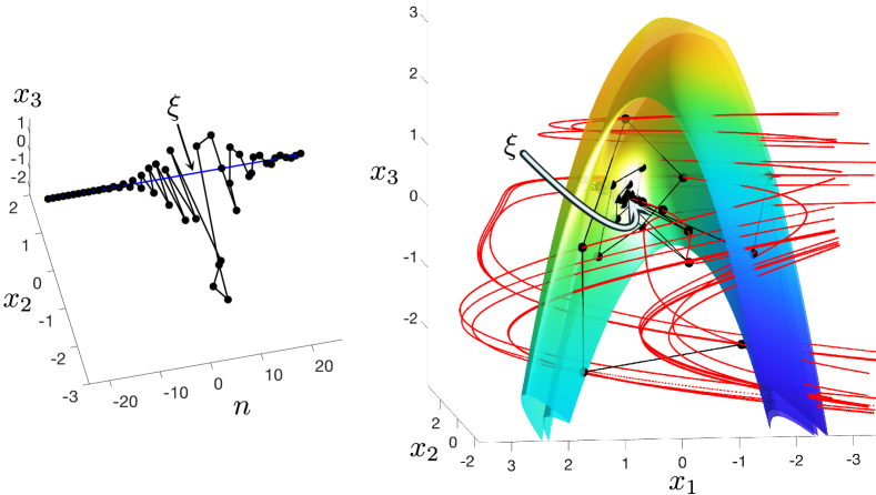
Figure 6: Center part of a homoclinic orbit of (59) (left). The same orbit in phase space (right) with approximations of unstable (red) and stable manifolds of $\xi$.

3.4 Almost periodicity and outer angular spectrum

The property of almost periodicity is a well-known concept to analyze the long time behavior of sequences which converge to some periodic orbit or to some ergodic motion on a circle; see [23, Ch.4.1] for the general theory. In [6] we have used this property to establish the existence and the equality of various angular values from Definition 2.6. In the following we study the sequence of maps

(64) $$b_{n}\colon\mathcal{G}(s,d)\to\mathbbm{R},\quad b_{n}(V)=\measuredangle(\Phi(n-1,0)V,\Phi(n,0)V),$$

from which the averages $\alpha_{n}=\frac{1}{n}\sum_{j=1}^{n}b_{j}(V)$ in (4) are derived. For example, we have shown in [6, Lemma 3.6, Proposition 3.7] that uniform almost periodicity (Uap) of the sequence $b_{n}$ implies the Cauchy property for $\alpha_{n}$ uniformly in $V$. The Uap notion is slightly weaker than in [23, Ch.4.1] and is further weakened in the following definition.

Definition 3.24

Given a set $\mathcal{V}$ and a metric space $(\mathcal{W},d)$. A sequence of mappings $b_{n}:\mathcal{V}\to\mathcal{W}$, $n\in\mathbbm{N}$ is called

• asymptotically uniformly almost periodic (AUap) if

  (65) $$\forall\varepsilon>0\ \exists P\in\mathbbm{N}\ \exists L\in\mathbbm{N}:\forall V\in\mathcal{V}\ \forall\ell\in\mathbbm{N}\ \exists p\in\{\ell,\dots,\ell+P\}:$$

  $$\forall n\geq L:d(b_{n}(V),b_{n+p}(V))\leq\varepsilon.$$

• uniformly almost periodic (Uap) if it is AUap with $L=1$.

Remark 3.25

Recall from [23, Ch.4.1] the standard definition of uniform almost periodicity for $b_{n}$: for every $\varepsilon>0$ there exists a relatively dense set $\mathcal{P}\subset\mathbbm{N}$ such that $|b_{n}(V)-b_{n+p}(V)|\leq\varepsilon$ for all $n\in\mathbbm{N},p\in\mathcal{P},V\in\mathcal{V}$; the set $\mathcal{P}$ is relatively dense iff there exists $P>0$ such that $\mathcal{P}\cap\{\ell,\ldots,\ell+P\}\neq\emptyset$ for all $\ell\in\mathbbm{N}$. Recall from [6, Remark 3.5] that Uap is weaker since we allow $p\in\{\ell,\ldots,\ell+P\}$ to depend on $V\in\mathcal{V}$, and note that AUap is still weaker since the estimate holds for $n\geq L$ only.

Definition 3.24 applies to dynamical systems of the form (1) with the setting $\mathcal{V}=\mathcal{W}=\mathcal{G}(s,d)$, $b_{n}(V)=\Phi(n,0)V$ and the metric $\measuredangle(\cdot,\cdot)$, but likewise to $\mathcal{V}=\mathcal{G}(s,d)$, $W=\mathbbm{R}$ and $b_{n}(V)=\measuredangle(\Phi(n,0)V,\Phi(n-1,0)V)$ for $n\geq 1$.

First note that (A)Uap carries over from subspaces to angles of successive subspaces.

Lemma 3.26

If $\varphi_{n}:\mathcal{G}(s,d)\to\mathcal{G}(s,d)$, $\varphi_{n}(V)=\Phi(n,0)V$ ($n\in\mathbbm{N}_{0}$) is (A)Uap in the metric space $(\mathcal{G}(s,d),\measuredangle(\cdot,\cdot))$, then the sequence of mappings

$$b_{n}:\mathcal{G}(s,d)\to\mathbbm{R},\quad b_{n}(V)=\measuredangle(\Phi(n-1,0)V,\Phi(n,0)V),\quad n\in\mathbbm{N}$$

is (A)Uap.

Proof 3.27

Given $\varepsilon>0$, choose $P$ and $L$ as in (65) w.r.t. $\frac{\varepsilon}{2}$. For $n\geq L$ then use the triangular inequality for the angle:

$$\big{|}\measuredangle(\Phi(n-1,0)V,\Phi(n,0)V)-\measuredangle(\Phi(n+p-1,0)V,\Phi(n+p,0)V)\big{|}$$

$$\leq\measuredangle(\Phi(n-1,0)V,\Phi(n+p-1,0)V)+\measuredangle(\Phi(n,0)V,\Phi(n+p,0)V)$$

$$\leq\tfrac{\varepsilon}{2}+\tfrac{\varepsilon}{2}=\varepsilon,$$

and the proof is complete. The case Uap follows by setting $L=1$.

Next we observe that the (A)Uap-property is invariant under kinematic transformations.

Proposition 3.28

Assume that the system (1) is AUap resp. Uap.
Then the kinematically equivalent system (33) is also AUap resp. Uap provided the transformations $Q_{n},Q_{n}^{-1}$ are uniformly bounded.

Proof 3.29

Let $\|Q_{m}\|\|Q_{n}^{-1}\|\leq\kappa$ for $n,m\in\mathbbm{N}$ and recall the constants $C=\pi\kappa(1+\kappa)$ from (82) and $C_{\pi}$ from (83). Given $\varepsilon>0$, choose $P$ and $L$ such that (65) holds with $\varepsilon^{\prime}=\frac{\varepsilon}{2CC_{\pi}(1+\kappa)}$ for $n-1\geq L$. By (34) the quantities $\tilde{b}_{n}$ which belong to $\tilde{\Phi}$ satisfy

$$\tilde{b}_{n}(Q_{0}V)=\measuredangle(\tilde{\Phi}(n-1,0)Q_{0}V,\tilde{\Phi}(n,0)Q_{0}V)=\measuredangle(Q_{n-1}\Phi(n-1,0)V,Q_{n}\Phi(n,0)V).$$

With Lemmas I.1, I.2 we then obtain from (65) for all $V\in\mathcal{G}(s,d)$, $\ell\in\mathbbm{N}$, $n\geq L$ and some $p\in\{\ell,\ldots,\ell+P\}$

$$|\tilde{b}_{n}(Q_{0}V)-\tilde{b}_{n+p}(Q_{0}V)|$$

$$=|\measuredangle(Q_{n-1}\Phi(n-1,0)V,Q_{n}\Phi(n,0)V)-\measuredangle(Q_{n+p-1}\Phi(n+p-1,0)V,Q_{n+p}\Phi(n+p,0)V)|$$

$$\leq\measuredangle(Q_{n-1}\Phi(n-1,0)V,Q_{n+p-1}\Phi(n+p-1,0)V)+\measuredangle(Q_{n}\Phi(n,0)V,Q_{n+p}\Phi(n+p,0)V)$$

$$\leq C\left[\measuredangle(Q_{n+p-1}^{-1}Q_{n-1}\Phi(n-1,0)V,\Phi(n+p-1,0)V)+\|Q_{n+p}^{-1}Q_{n}\Phi(n,0)V,\Phi(n+p,0)V)\right]$$

$$\leq CC_{\pi}\left[\|Q_{n+p-1}^{-1}Q_{n-1}-I\|\measuredangle(\Phi(n-1,0)V,\Phi(n+p-1,0)V)\right.$$

$$\left.\qquad\quad+\|Q_{n+p}^{-1}Q_{n}-I\|\measuredangle(\Phi(n,0)V,\Phi(n+p-1,0)V)\right]$$

$$\leq CC_{\pi}(1+\kappa)2\varepsilon^{\prime}=\varepsilon.$$

Note that this property allows us to obtain the AUap property for the $\ell^{1}$-perturbation of a system which has the AUap and the CED property; see Theorems 3.18 and 3.20.

The following Lemma 3.30 shows that the partial sums formed from an AUap sequence $b_{n}:\mathcal{V}\to\mathcal{W}$, $n\in\mathbbm{N}$ have the uniform Cauchy property. This extends [6, Lemma 3.6] where Uap was assumed. The property will be useful for deriving convergence of the numerical methods in Section 4. The proof is given in Appendix III.

Lemma 3.30

Let $b_{n}:\mathcal{V}\to\mathcal{W}$, $n\in\mathbbm{N}$ be a sequence of AUap and uniformly bounded functions. Then for all $\varepsilon>0$ there exists $N\in\mathbbm{N}$ such that for all $n\geq m\geq N$, $k\in\mathbbm{N}$, $V\in\mathcal{V}$

$$\Big{\|}\frac{1}{n}\sum_{j=1}^{n}b_{j}(V)-\frac{1}{m}\sum_{j=1}^{m}b_{j+k}(V)\Big{\|}\leq\varepsilon.$$

Example 3.31

(Example 3.9 revisited)
Consider the autonomous case $A_{n}\equiv A$ where $A$ is invertible and (complex) diagonalizable. Let $\lambda_{j}=\sigma_{j}e^{i\varphi_{j}}$, $\sigma_{j}>0$, $\varphi_{j}\in(0,\pi)$, $j=1,\ldots,k$ be the complex eigenvalues and let $\lambda_{j+k}\neq 0$, $j=1,\ldots\ell$ be the real ones (hence $d=2k+\ell$). We claim that the sequence

$$b_{n}:\mathcal{D}(s,d)\to\mathbbm{R},\quad b_{n}(V)=\measuredangle(A^{n-1}V,A^{n}V),\;n\in\mathbbm{N}$$

is Uap if the angles $\varphi_{j}$, $j=1,\ldots,k$ and $\pi$ are rationally independent, i.e.  $\sum_{j=1}^{k}n_{j}\varphi_{j}=n_{0}\pi$ for some $n_{j}\in\mathbbm{Z}$, $j=0,\ldots,k$ implies $n_{0}=n_{1}=\cdots=n_{k}=0$. Recall the Definition 2.17 of the trace space and note that $\mathcal{D}_{n}(s,d)\equiv\mathcal{D}(s,d)$ for all $n\in\mathbbm{N}$ in the autonomous case. By assumption there exists a decomposition $\mathbbm{R}^{d}=\bigoplus_{j=1}^{k+\ell}W_{j}$ into invariant subspaces of $A$ where $W_{j}=\mathcal{R}(Q_{j})$, $j=1,\ldots,k+\ell$ for matrices of full rank $Q_{j}\in\mathbbm{R}^{d,2},j=1,\ldots,k$ and $Q_{j+k}\in\mathbbm{R}^{d,1},j=1,\ldots,\ell$. Further, we have

(66) $$AQ_{j}=\sigma_{j}Q_{j}T_{\varphi_{j}},\ j=1,\ldots,k,\quad AQ_{j+k}=\lambda_{j+k}Q_{j+k},\ j=1,\ldots,\ell.$$

For every trace space $V\in\mathcal{D}(s,d)$ there exist subspaces $V_{j}$ of $W_{j}$, $j=1,\ldots,k+\ell$ (possibly trivial $V_{j}=\{0\}$) such that

$$V=\bigoplus_{j=1}^{k+\ell}V_{j},\quad\sum_{j=1}^{k+\ell}\dim(V_{j})=s.$$

The index set $J=\{j\in\{1,\ldots,k\}:\dim(V_{j})=1\}$ singles out the one-dimensional parts of $V$ in two-dimensional spaces so that $V_{j}=\mathrm{span}(v_{j})$ for some $v_{j}=Q_{j}u_{j}$, $\|u_{j}\|=1$, $j\in J$. For $j\notin J$ either $V_{j}=W_{j}$ or $V_{j}=\{0\}$ holds and, therefore, $AV_{j}=V_{j}$ follows from (66). On the other hand, equation (66) implies

$$AV_{j}=\mathrm{span}(Av_{j})=\mathrm{span}(Q_{j}T_{\varphi_{j}}u_{j}),\quad\text{ for }j\in J.$$

Next, consider the $|J|$-dimensional torus $\mathbbm{T}^{J}=\{u_{J}=(u_{j})_{j\in J}:u_{j}\in\mathbbm{R}^{2},\|u_{j}\|=1,j\in J\}$ and the maps

$$F_{J} :\mathbbm{T}^{J}\to\mathbbm{T}^{J},\quad F_{J}(u_{J})=(T_{\varphi_{j}}u_{j})_{j\in J},$$

$$g :\mathbbm{T}^{J}\to\mathbbm{R},\qquad\,g(u_{J})=\measuredangle\Big{(}\bigoplus_{j\in J}\mathrm{span}(Q_{j}u_{j})\oplus\bigoplus_{j\notin J}V_{j},\bigoplus_{j\in J}\mathrm{span}(Q_{j}T_{\varphi_{j}}u_{j})\oplus\bigoplus_{j\notin J}V_{j}\Big{)}.$$

With these settings we find $g(u_{J})=\measuredangle(V,AV)$, $g(F_{J}(u_{J}))=\measuredangle(AV,A^{2}V)$, and thus

$$b_{n}(V)=g(F_{J}^{n-1}(u_{J})),\quad\alpha_{n}(V)=\frac{1}{n}\sum_{j=1}^{n}b_{j}(V)=\frac{1}{n}\sum_{j=1}^{n}g(F_{J}^{j-1}(u_{J})).$$

Due to the rational independence of $\pi$ and $\varphi_{j}$, $j=1,\ldots,k$ the map $F_{J}$ is ergodic w.r.t. Lebesgue measure; see [19, Prop.1.4.1]. Moreover, $F_{J}$ is an isometry w.r.t. the metric $d(u_{J},v_{J})=\max_{j\in J}\measuredangle(u_{j},v_{j})$ on $\mathbbm{T}^{J}$. The result in [23, Ch. 4, Remark 1.3] then shows that the map $F_{J}$ is uniformly almost periodic i.e. for every $\varepsilon>0$ there exists a relatively dense set $\mathcal{P}\subset\mathbbm{N}_{0}$ with $d(u_{J},F_{J}^{p}(u_{J}))\leq\varepsilon$ for all $u_{J}\in\mathbbm{T}^{J}$, $p\in\mathcal{P}$. We prove that $b_{n}$ is then Uap on the set $\mathcal{D}_{J}(s,d)=\{V\in\mathcal{D}(s,d):\dim(V_{j})=1\text{ for }j\in J\}$ as follows (cf. the proof of [6, Proposition 5.2]): by the uniform continuity of $g$ on $\mathbbm{T}^{J}$ there exists for every $\varepsilon^{\prime}>0$ some $\varepsilon>0$ such that $|g(u_{J})-g(v_{J})|\leq\varepsilon^{\prime}$ whenever $d(u_{J},v_{J})\leq\varepsilon$, $u_{J},v_{J}\in\mathbbm{T}^{J}$. For the relatively dense set $\mathcal{P}$ which belongs to $\varepsilon$ we then obtain

$$|b_{n}(V)-b_{n+p}(V)|=|g(F_{J}^{n-1}(u_{J}))-g(F_{J}^{p}(F_{J}^{n-1}(u_{J})))|\leq\varepsilon^{\prime}\quad\forall n\in\mathbbm{N},p\in\mathcal{P},u_{J}\in\mathbbm{T}^{J}.$$

Thus $b_{n}$ is Uap on $\mathcal{D}_{J}(s,d)$ and also on $\mathcal{D}(s,d)=\bigcup_{J}\mathcal{D}_{J}(s,d)$, since there are only finitely many index sets $J\subseteq\{1,\ldots,k\}$.

The following example shows that the AUap property does not hold for matrices $A$ which have generalized eigenvectors.

Example 3.32

For the Jordan matrix $A=\left(\begin{smallmatrix}1&1\\ 0&1\end{smallmatrix}\right)$ the sequence $b_{n}(V)=\measuredangle(A^{n-1}V,A^{n}V)$, $V\in\mathcal{G}(1,2)$ is not AUap. Suppose the contrary and let $P,L$, $p=p(\ell,V)\in\{\ell,\ldots,\ell+P\}$ be the data from (65) with $\varepsilon=\frac{\pi}{8}$. For the vectors $v_{n}=\begin{pmatrix}-n+1&1\end{pmatrix}^{\top}$, $n\geq L$ we obtain

$$A^{n-1}v_{n}=\begin{pmatrix}0\\ 1\end{pmatrix},\quad A^{n}v_{n}=\begin{pmatrix}1\\ 1\end{pmatrix},\quad A^{n+p-1}v_{n}=\begin{pmatrix}p\\ 1\end{pmatrix},\quad A^{n+p}v_{n}=\begin{pmatrix}p+1\\ 1\end{pmatrix}.$$

Then we have $b_{n}(v_{n})=\measuredangle(A^{n-1}v_{n},A^{n}v_{n})=\frac{\pi}{4}$ and

$$b_{n+p(\ell,V_{n})}(v_{n})=\measuredangle\left(\begin{pmatrix}p(\ell,v_{n})\\ 1\end{pmatrix},\begin{pmatrix}p(\ell,v_{n})+1\\ 1\end{pmatrix}\right)\rightarrow 0\text{ as }\ell\to\infty$$

since $p(\ell,v_{n})\to\infty$ as $\ell\to\infty$. Thus $|b_{n}(v_{n})-b_{n+p(\ell,v_{n})}(v_{n})|\leq\frac{\pi}{8}$ is violated for $\ell$ sufficiently large.

Contrary to the (A)Uap-property, the uniform Cauchy (70) property is generally not invariant w.r.t. an autonomous similarity transformation as the following Example 3.33 shows.

Example 3.33

Let

$$D=\begin{pmatrix}J&0\\ 0&J\end{pmatrix},\quad J=\begin{pmatrix}0&-1\\ 1&0\end{pmatrix},\quad X=\begin{pmatrix}0&I_{2}\\ I_{2}&0\end{pmatrix}$$

and let $A_{n}$ be defined in Table 2. Denote by $\Phi$ the corresponding solution operator.

$n$	0	1	2	3	4	5	6	7	8	…	15	16	17	…	32	33
$A_{n}$	$D$	$D$	$X$	$D$	$D$	$D$	$D$	$X$	$D$	$\dots$	$D$	$X$	$D$	…	$D$	$X$

Table 2: Construction of $(A_{n})_{n\in\mathbbm{N}_{0}}$.

We analyze the case $s=1$. Since $\measuredangle(v,Dv)=\frac{\pi}{2}$ for each $0\neq v\in\mathbbm{R}^{4}$ we observe, that the system $u_{n+1}=A_{n}u_{n}$, $n\in\mathbbm{N}_{0}$ satisfies the uniformly Cauchy condition (70).

Let

$$B_{n}=SA_{n}S^{-1}\quad\text{with}\quad S=\begin{pmatrix}1&0&0&0\\ 0&1&0&0\\ 0&0&1&1\\ 0&0&0&1\end{pmatrix}.$$

Denote by $e_{i}$ the $i$-th unit vector. We get

$$\measuredangle(Sv,SDv)=\begin{cases}\tfrac{\pi}{2},&\text{for }v\in\{e_{1},e_{2}\},\\ \tfrac{\pi}{4},&\text{for }v\in\{e_{3},e_{4}\}.\end{cases}$$

For $v=e_{1}$, the sequence $\frac{1}{n}\sum_{j=1}^{n}\measuredangle(S\Phi(j-1,0)v,S\Phi(j,0)v)$, $n\in\mathbbm{N}$ does not converge and thus, the transformed system does not satisfy (70).

4 Numerical approximation

In [8, Section 4.1] we developed an algorithm for the approximation of outer angular values. In Section 4.2 we extend these ideas and obtain an algorithm that approximates the outer angular spectrum $\Sigma_{s}$. In Section 4.1 we introduce finite time outer angular spectra and investigate their lower and upper semi-continuity.

4.1 Convergence of finite time angular spectra

For the numerical calculation of $\Sigma_{s}$, we introduce the finite time outer angular $N$-spectrum

$$\Sigma_{s}^{N}\coloneqq\{\alpha_{N}(V):V\in\mathcal{D}_{0}(s,d)\}.$$

This spectrum is numerically accessible by computing the dichotomy spectrum and its spectral bundles first, and then by solving optimization problems. For the simple Example 2.20, finite time and infinite outer angular spectra coincide, i.e. $\Sigma_{s}=\Sigma_{s}^{N}$ for $s\in\{1,2\}$ and all $N\in\mathbbm{N}$.

We observe the following (modest) connection between these spectra.

Lemma 4.1

For every $\varepsilon>0$ and $\theta\in\Sigma_{s}$ there exists some $N\in\mathbbm{N}$ sucht that

$${\rm{dist}}(\theta,\Sigma_{s}^{N})\leq\varepsilon.$$

Proof 4.2

Let $\varepsilon>0$ and $\theta\in\Sigma_{s}$. Then, there exists a $V\in\mathcal{D}_{0}(s,d)$ such that

$$\theta\in[\varliminf_{n\to\infty}\alpha_{n}(V)-\tfrac{\varepsilon}{2},\varlimsup_{n\to\infty}\alpha_{n}(V)+\tfrac{\varepsilon}{2}].$$

By Lemma 2.4, each angle in $[\varliminf_{n\to\infty}\alpha_{n}(V),\varlimsup_{n\to\infty}\alpha_{n}(V)]$ is an accumulation point of $(\alpha_{n}(V))_{n\in\mathbbm{N}}$. Thus, we find an $N\in\mathbbm{N}$ such that $|\alpha_{N}(V)-\theta|\leq\varepsilon$.

However, finite and infinite spectra do not conicide in general. We revisit the key examples from [6, Section 3.2]. These examples show that one can generally not expect a sharper result than Lemma 4.1. The well known notions of upper semi-continuity and lower semi-continuity do not hold true.

Example 4.3

For given $0\leq\varphi_{0}<\varphi_{1}\leq\frac{\pi}{2}$ we define

(67) $$A_{n}=\begin{cases}T_{\varphi_{0}},&\text{ for }n=0\lor n\in\bigcup_{\ell=1}^{\infty}[2^{2\ell-1},2^{2\ell}-1]\cap\mathbbm{N},\\[8.53581pt] T_{\varphi_{1}},&\text{ otherwise.}\end{cases}$$

Following the computation of the extremal values in [6, Example 3.10] we obtain the outer angular spectra

$$\Sigma_{1}=\big{[}\tfrac{2}{3}\varphi_{0}+\tfrac{1}{3}\varphi_{1},\tfrac{1}{3}\varphi_{0}+\tfrac{2}{3}\varphi_{1}\big{]},\quad\Sigma_{1}^{N}=\{\alpha_{N}(V):V\in\mathcal{G}(1,2)\}.$$

Note that the dichotomy spectrum $\{1\}$ provides no spectral separation, i.e. $\mathcal{W}_{0}^{1}=\mathbbm{R}^{2}$. Thus we find $\mathcal{D}_{0}(1,2)=\mathcal{G}(1,2)$. All one-dimensional subspaces lead to the same angular value w.r.t. (67). For every fixed $V\in\mathcal{G}(1,2)$ we get

$$\Sigma_{1}^{N} =\{\alpha_{N}(V)\}=\Big{\{}\frac{1}{N}\sum_{j=1}^{N}\measuredangle(\Phi(j-1,0)V,\Phi(j,0)V)\Big{\}}=\Big{\{}\frac{1}{N}\sum_{j=1}^{N}g(j)\Big{\}}$$

where

$$g(j)=\begin{cases}\varphi_{0},&\text{ for }j=0\lor j\in\bigcup_{\ell=1}^{\infty}[2^{2\ell-1},2^{2\ell}-1]\cap\mathbbm{N},\\[8.53581pt] \varphi_{1},&\text{ otherwise.}\end{cases}$$

The finite time outer angular spectrum $\Sigma_{1}^{N}$ consists of one element only for each $N\in\mathbbm{N}$ and, therefore, cannot approximate the interval $\Sigma_{1}$.

This example shows that Lemma 4.1 does not imply lower semi-continuity, i.e.

$${\rm{dist}}(\Sigma_{1},\Sigma_{1}^{N})=\sup_{\theta\in\Sigma_{1}}\inf_{\vartheta\in\Sigma_{1}^{N}}|\theta-\vartheta|\to 0\text{ as }N\to\infty.$$

However, lower semi-continuity can be achieved for the union of finite time spectral sets. For $N,M\in\mathbbm{N}$, $N<M$ we define

(68) $$\Sigma_{s}^{N,M}\coloneqq\bigcup_{j=N}^{M}\Sigma_{s}^{j}$$

and get lower semi-continuity in the following sense:

Lemma 4.4

For any $N\in\mathbbm{N}$ the following holds:

$$\lim_{M\to\infty}{\rm{dist}}\left(\Sigma_{s},\Sigma_{s}^{N,M}\right)=0.$$

Proof 4.5

Let us denote by $B_{\varepsilon}(X)=\{y\in\mathbbm{R}:{\rm{dist}}(y,X)\leq\varepsilon\}$ the $\varepsilon$-neighborhood of a set $X\subseteq\mathbbm{R}$ . Fix $N\in\mathbbm{N}$ and $\varepsilon>0$. Similar to the proof of Lemma 4.1, we find for each $\theta\in\Sigma_{s}$ an element $V\in\mathcal{D}_{0}(s,d)$ such that

$$B_{\frac{\varepsilon}{4}}(\theta)\subset[\varliminf_{n\to\infty}\alpha_{n}(V)-\tfrac{\varepsilon}{2},\varlimsup_{n\to\infty}\alpha_{n}(V)+\tfrac{\varepsilon}{2}].$$

Since $\lim_{n\to\infty}\alpha_{n}(V)-\alpha_{n+1}(V)=0$, we obtain a number $L=L(\theta)\geq N$ such that $B_{\frac{\varepsilon}{4}}(\theta)\subset B_{\varepsilon}(\alpha_{L(\theta)}(V))$ and thus $B_{\frac{\varepsilon}{4}}(\theta)\subset B_{\varepsilon}(\Sigma_{s}^{L(\theta)})$.

Since $\Sigma_{s}$ is compact there exist some $\ell\in\mathbbm{N}$ and $\theta_{1},\dots,\theta_{\ell}\in\Sigma_{s}$ such that $\Sigma_{s}\subseteq\bigcup_{j=1}^{\ell}B_{\frac{\varepsilon}{4}}(\theta_{j})$. Let $M=\max_{j=1,\dots,\ell}L(\theta_{j})$. Then we get for all $\theta\in\Sigma_{s}$:

$$\theta\in\bigcup_{j=N}^{M}B_{\varepsilon}\left(\Sigma_{s}^{j}\right)=B_{\varepsilon}\Big{(}\bigcup_{j=N}^{M}\Sigma_{s}^{j}\Big{)}=B_{\varepsilon}\left(\Sigma_{s}^{N,M}\right)$$

and

$${\rm{dist}}\left(\Sigma_{s},\Sigma_{s}^{N,M}\right)=\sup_{\theta\in\Sigma_{s}}\inf_{\vartheta\in\Sigma_{s}^{N,M}}|\theta-\vartheta|\leq\varepsilon.$$

The next example shows that the finite time outer angular spectra can be much larger than the infinite ones.

Example 4.6

Consider the system (1) with the following setting:

(69) $$A_{n}\coloneqq\begin{cases}\left(\begin{smallmatrix}-1&0\\ 0&1\end{smallmatrix}\right),&\text{ for }n\in\bigcup_{\ell=1}^{\infty}[2\cdot 2^{\ell}-4,3\cdot 2^{\ell}-5],\\ \left(\begin{smallmatrix}1&0\\ 0&\frac{1}{2}\end{smallmatrix}\right),&\text{ otherwise.}\end{cases}$$

It turns out that $\Sigma_{1}=\{0\}$ and we determine $\Sigma_{1}^{N}=\{\alpha_{1}(V):V\in\mathcal{G}(1,d)\}$. For a fixed $N\in\mathbbm{N}$ there exists $\varepsilon>0$ such that

$$\alpha_{N}\left({\mathrm{span}}\begin{pmatrix}0\\ 1\end{pmatrix}\right)=0,\quad\alpha_{N}\left({\mathrm{span}}\begin{pmatrix}\varepsilon\\ 1\end{pmatrix}\right)\geq\frac{\pi}{12}.$$

By the continuity of $\alpha_{N}$ we obtain $\Sigma_{1}^{N}\supseteq[0,\frac{\pi}{12}]$ which is much larger than the outer angular spectrum $\Sigma_{1}$. In particular, there seems to be no easy relation between $\Sigma_{s}$ and $\Sigma_{s}^{N}$.

Example 4.6 shows that Lemma 4.1 does not imply upper semi-continuity, i.e.

$${\rm{dist}}(\Sigma_{1}^{N},\Sigma_{1})=\sup_{\theta\in\Sigma_{1}^{N}}\inf_{\vartheta\in\Sigma_{1}}|\theta-\vartheta|\to 0\text{ as }N\to\infty.$$

For each $N\in\mathbbm{N}$ we find ${\rm{dist}}(\Sigma_{1}^{N},\Sigma_{1})=\sup_{\theta\in\Sigma_{1}^{N}}|\theta|\geq\tfrac{\pi}{12}$. We also do not get upper semi-continuity when replacing $\Sigma_{1}^{N}$ by $\Sigma_{1}^{N,M}$. In the following we look for stronger assumptions which guarantee upper semi-continuity. Recall from Lemma 3.30 the uniform Cauchy property, i.e. the sequence $\alpha_{N}(V)$ satisfies

(70) $$\forall\varepsilon>0\ \exists N=N(\varepsilon)\in\mathbbm{N}:\forall n,m\geq N:\forall V\in\mathcal{D}_{0}(s,d):|\alpha_{n}(V)-\alpha_{m}(V)|\leq\varepsilon.$$

Lemma 4.7

If the sequence $\alpha_{N}(V)$, $V\in\mathcal{G}(s,d)$, $N\in\mathbbm{N}$ is uniformly Cauchy then upper semi-continuity holds true in the following sense:

(71) $$\forall\varepsilon>0\ \exists N\in\mathbbm{N}:\forall M\geq N:{\rm{dist}}(\Sigma_{s}^{N,M},\Sigma_{s})\leq\varepsilon.$$

Proof 4.8

The uniform Cauchy property implies

(72) $$\forall\varepsilon>0\ \exists\bar{N}\in\mathbbm{N}:\forall N\geq\bar{N}\ \forall V\in\mathcal{D}_{0}(s,d):\alpha_{N}(V)\in B_{\varepsilon}\left(\lim_{n\to\infty}\alpha_{n}(V)\right).$$

Thus, if we fix $N=\bar{N}(\varepsilon)$ as in (72) and let $M\geq N$, then for every $\theta\in\Sigma_{s}^{N,M}$ there exist a $V\in\mathcal{D}_{0}(s,d)$ and an index $j\in[N,M]\cap\mathbbm{N}$ such that $\theta=\alpha_{j}(V)$, hence

$$\theta\in B_{\varepsilon}(\lim_{n\to\infty}\alpha_{n}(V))\subset B_{\varepsilon}(\Sigma_{s}).$$

This proves our assertion.

Remark 4.9

Note that lower semi-continuity requires only the index $M$ in $\Sigma_{s}^{N,M}$ to be large while upper semi-continuity also needs $N$ to be sufficiently large.

The uniform Cauchy property even guarantees that the finite time angular spectra converge in the Hausdorff distance without forming the union (68).

Proposition 4.10

If the uniform Cauchy condition (70) is satisfied then convergence holds w.r.t. the Hausdorff distance, i.e.

(73) $$\forall\varepsilon>0\ \exists N\in\mathbbm{N}:\forall n\geq N:d_{H}(\Sigma_{s},\Sigma_{s}^{n})\leq\varepsilon,$$

where $d_{H}(U,V)\coloneqq\max\{{\rm{dist}}(U,V),{\rm{dist}}(V,U)\}$.

Proof 4.11

Given $\varepsilon>0$ choose $N\in\mathbbm{N}$ such that

(74) $$|\alpha_{n}(V)-\lim_{\ell\to\infty}\alpha_{\ell}(V)|\leq\frac{\varepsilon}{2}\quad\forall n\geq N,\ \forall V\in\mathcal{D}_{0}(s,d).$$

Consider now $n\geq N$:

• For $\theta\in\Sigma_{s}^{n}$ we find some $V\in\mathcal{D}_{0}(s,d)$ such that $\alpha_{n}(V)=\theta$. Since $\lim_{\ell\to\infty}\alpha_{\ell}(V)\in\Sigma_{s}$ the property (74) shows ${\rm{dist}}(\Sigma_{s}^{n},\Sigma_{s})\leq\frac{\varepsilon}{2}$.

• For $\theta\in\Sigma_{s}$ we find a $V\in\mathcal{D}_{0}(s,d)$ such that $|\theta-\lim_{\ell\to\infty}\alpha_{\ell}(V)|\leq\frac{\varepsilon}{2}$. With our choice of $N$ and $n$ in (74) we obtain

  $$|\theta-\alpha_{n}(V)|\leq|\theta-\lim_{\ell\to\infty}\alpha_{\ell}(V)|+|\lim_{\ell\to\infty}\alpha_{\ell}(V)-\alpha_{n}(V)|\leq\frac{\varepsilon}{2}+\frac{\varepsilon}{2}=\varepsilon.$$

  Thus we have shown that ${\rm{dist}}(\Sigma_{s},\Sigma_{s}^{n})\leq\varepsilon$ follows.

Combining both results proves (73).

According to this result we can determine the outer angular spectrum of a system (1) in an efficient way if it is uniformly Cauchy. It suffices to calculate $\Sigma_{s}^{n}$ for $n$ sufficiently large, while systems without this property require to compute the union of several sets $\Sigma_{s}^{N,M}$ with $M\geq N$.

Let us recall from Section 3 that the uniform Cauchy property is implied by uniform almost periodicity of the sequence $b_{n}(V)=\measuredangle(\Phi(n-1,0)V,\Phi(n,0)V)$ (Lemma 3.30). The last property, in turn, holds for autonomous systems where the matrix $A$ has semi-simple eigenvalues and the frequencies satisfy a nonresonance condition (Example 3.31). Moreover, this property is inherited by kinematically similar systems (Proposition 3.28). Among these kinematically similar systems are those for which the system matrices $A_{n}$ are $\ell^{1}$-perturbations of $A$ (Theorem 3.7). This theorem needs the CED property which follows if the matrix $A$ has only semi-simple eigenvalues; see Example 3.9. Summing all up, we find that the approximation result in Proposition 4.10 applies to the $3$D-Hénon system from Example 3.23 for which the nonresonance condition is trivially satisfied.

4.2 An algorithm for computing the finite time outer angular $N$-spectrum

We know turn the definition of the finite time outer angular spectrum into an algorithm, having in mind our main application – the $3$D-Hénon map from Example 3.23. By Proposition 4.10 it suffices to compute the finite time outer angular $N$-spectrum for sufficiently large $N$ in case $s\in\{1,2\}$ since $\Sigma_{s}^{N}$ converges to $\Sigma_{s}$ w.r.t. the Hausdorff distance. In particular, all limits exist.

We assume that $\dim(\mathcal{W}_{0}^{k})\in\{1,2\}$ for all $k=1,\dots,\varkappa$, cf. Definition 2.17. Fix $N\in\mathbbm{N}$ and for $V\in\mathcal{G}(s,d)$ we abbreviate

$$\theta_{s}(V)=\alpha_{N}(V)=\frac{1}{N}\sum_{j=1}^{N}\measuredangle(\Phi(j-1,0)V,\Phi(j,0)V),\quad\theta_{s}(v)=\theta_{s}(\mathrm{span}(v))$$

and define

$$\mathcal{B}_{0}^{k}=\{v\in\mathcal{W}_{0}^{k}:\|v\|=1\}\quad\text{for }k\in\{1,\dots,\varkappa\}.$$

Step 1: Computation of the dichotomy spectrum and of the spectral bundles

The computation of the dichotomy spectrum $\Sigma_{\mathrm{ED}}^{\mathrm{approx}}$ and of the corresponding spectral bundles is described in detail in [8, Section 4.1, Step 1 and 2]. In the following we use these techniques for approximating the fibers $\mathcal{W}_{0}^{k}$, $k=1,\dots,\varkappa$.

Step 2: Computation of the first finite time outer angular $N$-spectrum $\Sigma_{1}^{N}$

initialize $\Sigma_{1}^{N}=\emptyset$

for $k=1,\dots,\varkappa$ do

     if $\dim(\mathcal{W}_{0}^{k})=1$ then

         $\Sigma_{1}^{N}=\Sigma_{1}^{N}\cup\theta_{1}(\mathcal{W}_{0}^{k})$

     else

         $\displaystyle\Sigma_{1}^{N}=\Sigma_{1}^{N}\cup\left[\min_{v\in\mathcal{B}_{0}^{k}}\theta_{1}(v),\max_{v\in\mathcal{B}_{0}^{k}}\theta_{1}(v)\right]$

     end if

end for

Note that we solve one-dimensional optimization problems in case $\dim(\mathcal{W}_{0}^{k})=2$ with the MATLAB-routine fminbnd.

Step 3: Computation of the second finite time outer angular $N$-spectrum $\Sigma_{2}^{N}$

initialize $\Sigma_{2}^{N}=\emptyset$

for $k=1,\dots,\varkappa$ do

     if $\dim(\mathcal{W}_{0}^{k})=2$ then

         $\Sigma_{2}^{N}=\Sigma_{2}^{N}\cup\theta_{2}(\mathcal{W}_{0}^{k})$

     end if

end for

for $k_{1}=1,\dots,\varkappa-1$ do

     for $k_{2}=k_{1}+1,\dots,\varkappa$ do

         $\displaystyle\Sigma_{2}^{N}=\Sigma_{2}^{N}\cup\left[\min_{x\in\mathcal{B}_{0}^{k_{1}},y\in\mathcal{B}_{0}^{k_{2}}}\theta_{2}({\mathrm{span}}(x,y)),\max_{x\in\mathcal{B}_{0}^{k_{1}},y\in\mathcal{B}_{0}^{k_{2}}}\theta_{2}({\mathrm{span}}(x,y))\right]$

     end for

end for

The optimization problems that we solve in the last step have dimension $\dim(\mathcal{W}_{0}^{k_{1}})+\dim(\mathcal{W}_{0}^{k_{2}})-2$. For two-dimensional optimization problems, we apply the MATLAB-routine fminsearch.

4.3 Numerical results for the 3D-Hénon system

For $N\in\{50,100,1000,2000\}$, we apply the algorithm from above to the $3$D-Hénon systems (60), see Table 3 and to (61), cf. Table 4. Note that we shift the index in (60) such that the main excursion of the homoclinic orbit $\bar{x}_{0}$ lies at $\frac{N}{2}$.

Errors that occur while computing homoclinic orbits and the corresponding fiber bundles decay exponentially fast towards the midpoint of the finite interval, see [17, Section 2.6]. These errors can be neglected, if the orbit and the fibers are computed on sufficiently large intervals, while only the center part of length $N$ is used. For this task, we introduce left and right buffer intervals of length $500$, which are skipped in the final output.

$N$	$\Sigma_{\mathrm{ED}}^{\mathrm{approx}}$	$\Sigma_{1}^{N}$	$\Sigma_{2}^{N}$
$50$	$[0.775,0.787]\cup[1.467,1.482]$	$\{0.358\}\cup[1.108,1,264]$	$\{0.487\}\cup[1.211,1.275]$
$100$	$[0.776,0.785]\cup[1.468,1.482]$	$\{0.178\}\cup[1.222,1,307]$	$\{0.242\}\cup[1.289,1.296]$
$1000$	$[0.779,0.784]\cup[1.470,1.478]$	$\{0.018\}\cup[1.325,1,333]$	$\{0.024\}\cup[1.324,1.325]$
$2000$	$[0.779,0.784]\cup[1.471,1.477]$	$\{0.009\}\cup[1.330,1,331]$	$\{0.012\}\cup[1.326,1.327]$

Table 3: Numerical computation of the dichotomy spectrum and of outer angular spectra for the nonautonomous $3$D-Hénon system (60).

Note that for the autonomous system (61), trace spaces are eigenspaces. For a fair comparison however, we compute the trace spaces also in the autonomous setting with the more general nonautonomous algorithm.

$N$	$\Sigma_{\mathrm{ED}}^{\mathrm{approx}}$	$\Sigma_{1}^{N}$	$\Sigma_{2}^{N}$
$50$	$[0.781,0.782]\cup[1.473,1.474]$	$\{10^{-16}\}\cup[1.328,1,344]$	$\{10^{-16}\}\cup[1.320,1.337]$
$100$	$[0.781,0.782]\cup[1.473,1.474]$	$\{10^{-16}\}\cup[1.328,1,341]$	$\{10^{-16}\}\cup[1.321,1.334]$
$1000$	$[0.781,0.782]\cup[1.473,1.474]$	$\{10^{-16}\}\cup[1.335,1,336]$	$\{10^{-15}\}\cup[1.328,1.328]$
$2000$	$[0.781,0.782]\cup[1.473,1.474]$	$\{10^{-16}\}\cup[1.335,1,336]$	$\{10^{-15}\}\cup[1.328,1.328]$

Table 4: Numerical computation of the dichotomy spectrum and of outer angular spectra for the autonomous $3$D-Hénon system (61).

The data in Table 4 show that the finite time outer angular $N$-spectra depend on $N$. This causes $\rho\approx 0.697\neq 1$ in the normal form (8) that belongs to the two-dimensional eigenspace of $Df(\xi)$. However, these spectra converge quickly in $N$ towards the infinite time spectra (62) and (63), respectively.

Next, we discuss the results for the variational equation along the homoclinic orbit in Table 3. On the one hand, the center part of the homoclinic orbit, see Figure 2, has for small $N$ a strong influence on the finite time outer angular $N$-spectra. For sufficiently large $N$, on the other hand, $Df(\bar{x}_{n})$ is exponentially close to $Df(\xi)$, if $n$ lies at the boundaries of the finite interval $[0,N]\cap\mathbbm{N}_{0}$. Hence, the finite time outer angular $N$-spectra of both systems (61) and (60) converge for increasing $N$ towards each other. These observations are in line with the theoretical results from Section 4.1.

Figure 7: Distance of a homoclinic orbit$(\bar{x}_{n})_{n\in\{0,1,\dots,2000\}}$ of the $3$D-Hénon system (59) to the fixed point $\xi$ in a semilogarithmic scale.

4.4 Multi-humped homoclinic orbits for the 3D-Hénon system

While outer angular spectra of the variational equation along a homoclinic $3$D-Hénon orbit essentially depend only on the limit matrix $DF(\xi)$, the situation changes when we consider so called multi-humped homoclinic orbits, see [10]. We construct these orbits by copying the center part of length $M$ of the primary homoclinic orbit repeatedly, see Figure 8. Then Newton’s method, applied to this pseudo-orbit results in an $F$-orbit $(\bar{x}^{M}_{n})_{n\in J}$ on the finite interval $J=[0,2000]\cap\mathbbm{N}_{0}$.

Figure 8: Construction of multi-humped orbits.

For large $M$, the dynamics at the fixed point essentially determines the outer angular spectra. However, for small values of $M$, the multiple center parts of the primary homoclinic orbit alter the outer angular spectra, see Table 5. For $M\in\{50,100,200\}$ we observe that the dichotomy spectrum consists of three intervals, resulting in one-dimensional trace spaces. For $M=400$, the algorithm from [8, Section 4.1] no longer separates the values of the dichotomy spectrum and finds the interval $[0.773,0.788]$. This interval leads to a two-dimensional trace space and, as a consequence, intervals also occur in the outer angular spectra for $M=400$.

Passing from $M$ to $2M$, we further observe that any value within the outer angular spectrum $\Sigma_{1}^{2001}$ or $\Sigma_{2}^{2001}$ for $2M$ is roughly the arithmetic mean of the corresponding value for $M$ and the respective value from (62) and (63). In other words, the distance to the values from (62) and (63) is halved when $M$ is doubled. Such a behavior is suggested by the fact that orbits stay twice as long near the fixed point.

$M$ $\Sigma_{\mathrm{ED}}^{\mathrm{approx}}$ $50$ $[0.7230,0.7234]\cup[0.8298,0.8302]\cup[1.4992,1.4994]$ $100$ $[0.7492,0.7494]\cup[0.8077,0.8079]\cup[1.4868,1.4870]$ $200$ $[0.7634,0.7662]\cup[0.7935,0.7966]\cup[1.4775,1.4827]$ $400$ $[0.7733,0.7884]\cup[1.4741,1.4791]$

$M$ $\Sigma_{1}^{2001}$ $\Sigma_{2}^{2001}$ $50$ $\{0.353,1.135,1.260\}$ $\{0.480,1.248,1.264\}$ $100$ $\{0.177,1.229,1.300\}$ $\{0.239,1.295,1.296\}$ $200$ $\{0.088,1.281,1.318\}$ $\{0.120,1.312,1.313\}$ $400$ $\{0.044\}\cup[1.311,1.314]$ $\{0.060\}\cup[1.320,1.321]$

Table 5: Numerical computation of the dichotomy spectrum and of outer angular spectra for the $3$D-Hénon system w.r.t. multi-humped homoclinic orbits with center parts of length $M$.

4.5 Angular spectra for the Lorenz system

The famous Lorenz system [20] is given by the ODE

(75) $$\begin{pmatrix}y_{1}\\ y_{2}\\ y_{3}\end{pmatrix}^{\prime}=\begin{pmatrix}\sigma(y_{2}-y_{1})\\ \rho y_{1}-y_{2}-y_{1}y_{3}\\ y_{1}y_{2}-\beta y_{3}\end{pmatrix}\quad\text{with parameters}\quad\sigma=10,\ \rho=28,\ \beta=\tfrac{8}{3}.$$

In order to apply our results, we discretize this ODE and compute the $h$-step map $F_{h}$ for $h\in\{0.05,0.1,0.2\}$. For this task, we apply the classical Runge-Kutta scheme with step size $10^{-4}$. For the resulting discrete time system

(76) $$x_{n+1}=F_{h}(x_{n}),\quad n\in\mathbbm{N}_{0}$$

we calculate an orbit $(\bar{x}_{n})_{n\in\{0,\dots,11000\}}$ w.r.t. the initial value $\bar{x}_{0}=\begin{pmatrix}10&10&10\end{pmatrix}^{\top}$ that converges towards the Lorenz attractor. To the resulting variational equation

$$u_{n+1}=DF_{h}(\bar{x}_{n})u_{n},\quad n=0,\dots,11000$$

we apply the algorithm from Section 4.2 with left and right buffer intervals of length $500$. Here, the Jacobians $DF_{h}(\bar{x}_{n})$ are computed numerically using the central difference quotient. Table 6 gives the resulting spectra for $h\in\{0.05,0.1,0.2\}$.

$h$ $\Sigma_{\mathrm{ED}}^{\mathrm{approx}}$ $0.05$ $[0.4821,0.4833]\cup[0.9995,1.0005]\cup[1.0445,1.0478]$ $0.1$ $[0.2325,0.2332]\cup[0.9995,1.0007]\cup[1.0928,1.0971]$ $0.2$ $[0.0542,0.0544]\cup[0.9994,1.0006]\cup[1.1956,1.2004]$

$h$ $\Sigma_{1}^{10001}$ $\Sigma_{2}^{10001}$ $0.05$ $\{0.2039,0.3803,0.4234\}$ $\{0.0689,0.3604,0.4188\}$ $0.1$ $\{0.3925,0.7282,0.8268\}$ $\{0.1356,0.7021,0.8197\}$ $0.2$ $\{0.6552,0.7334,0.9727\}$ $\{0.2475,0.7934,0.9752\}$

Table 6: Dichotomy spectrum and angular spectra for the $h$-step Lorenz map w.r.t. an orbit on the Lorenz attractor.

We observe that spectral values of the dichotomy spectrum are squared when passing from $h$ to $2h$. For the corresponding values of the outer angular spectrum, we expect them to double for sufficient small $h$, while this doubling cannot be expected for larger values of $h$. This interpretation is in line with the numerical data in Table 6.

We shift the orbit outside the buffer intervals to $(\bar{x}_{n})_{n\in\{0,\dots,10^{4}\}}$ and illustrate the trace spaces $\mathcal{D}_{n}(1,3)=\{\mathcal{W}_{n}^{1},\mathcal{W}_{n}^{2},\mathcal{W}_{n}^{3}\}$ for $n=2400$ and $h=0.05$ in Figure 9.

Figure 9: Part of an $F_{0.05}$-orbit $(\bar{x}_{n})_{n\in\{2300,\dots,2500\}}$ (connected with lines) of the Lorenz system (76). For $n=2400$ the three trace spaces $\mathcal{W}_{n}^{1,2,3}$ are shown.

The trace space $\mathcal{W}_{n}^{2}$ lies in the direction of the flow of the ODE (75) and belongs to the spectral interval around $1$ of the dichotomy spectrum. Here the maximal value of the outer angular spectrum $0.4234$ is achieved. The trace space $\mathcal{W}_{n}^{1}$ also lies in the ‘plane’ of the attractor and leads to the spectral value $0.3803$. Finally, $\mathcal{W}_{n}^{3}$ points outside of the ‘plane’ of the attractor and gives the smallest value $0.2039$ of the outer angular spectrum.

The outer angular spectrum of dimension $s=2$ is calculated w.r.t. the trace spaces $\mathcal{D}_{n}(2,3)=\{\mathcal{W}_{n}^{1}\oplus\mathcal{W}_{n}^{2},\mathcal{W}_{n}^{1}\oplus\mathcal{W}_{n}^{3},\mathcal{W}_{n}^{2}\oplus\mathcal{W}_{n}^{3}\}$. The largest value $0.4188$ of $\Sigma_{2}$ is attained in $\mathcal{W}_{n}^{2}\oplus\mathcal{W}_{n}^{3}$ while $\mathcal{W}_{n}^{1}\oplus\mathcal{W}_{n}^{3}$ results in the angular value $0.3604$. The smallest value $0.0689$ is attained in the ‘plane’ of the attractor $\mathcal{W}_{n}^{1}\oplus\mathcal{W}_{n}^{2}$.

The angle between successive iterates of the $h$-step Lorenz map on average, as indicated in the upper right of Figure 9, is an alternative way to measure the rotation of a trajectory. The resulting values are given in Table 7. For sufficiently small $h$, these values turn out to be close to the largest spectral value of $\Sigma_{1}^{10001}$.

$h$	$0.05$	$0.1$	$0.2$
angle on average	$0.4227$	$0.8322$	$1.0993$

Table 7: Angle between successive iterates on average for the $h$-step Lorenz map (76).

Angular values for continuous time systems have been introduced in [9, Definition 4.3]. These normalized values are defined as

(77) $$\theta_{s,h,T}^{\mathrm{cont}}=\sup_{V\in\mathcal{D}_{0}(s,d)}\frac{1}{T}\sum_{j=1}^{N}\measuredangle(\Phi_{h}(j,0)V,\Phi_{h}(j-1,0)V),\quad N=\tfrac{T}{h},$$

where $T$ denotes the length of the time interval, $h$ the step size and $\Phi_{h}$ is the solution operator of the $h$-step Lorenz map. In the limit $h\to 0$, $\theta_{s,h,T}^{\mathrm{cont}}$ measures the average rotation of an $s$-dimensional subspace per unit time interval when observed during $T$ time units. When the time $T$ of observation tends to infinity we obtain an angular value of the continuous time system. Note that $\theta_{s,h,T}^{\mathrm{cont}}$ is not restricted to $[0,\frac{\pi}{2}]$, since a subspace may rotate multiple times on a time interval of length $1$. For the Lorenz system, the supremum in (77) is attained in $\mathcal{W}_{0}^{2}$ for $s=1$ and in $\mathcal{W}_{0}^{2}\oplus\mathcal{W}_{0}^{3}$ for $s=2$. In Table 8, we compute $\theta_{s,h,T}^{\mathrm{cont}}$ for $s\in\{1,2\}$, $T=500$ and $h\in\{0.025,0.05,0.1,0.2\}$. To ensure accurate results, additional left and right buffer intervals (in time) of length $T_{\mathrm{buffer}}=25$ are added. The data in Table 8 illustrate the convergence of $\theta_{s,h,T}^{\mathrm{cont}}$ as $h\to 0$ towards the angular value of the continuous system in finite time $T=500$.

$h$	$0.025$	$0.05$	$0.1$	$0.2$
$\theta_{1,h,T}^{\mathrm{cont}}$	$8.4798$	$8.4672$	$8.2896$	$4.8752$
$\theta_{2,h,T}^{\mathrm{cont}}$	$8.3816$	$8.3753$	$8.2209$	$4.8941$

Table 8: Normalized angular values $\theta_{1,h,T}^{\mathrm{cont}}$ and $\theta_{2,h,T}^{\mathrm{cont}}$ for the $h$-step Lorenz map (76).

5 Further types of angular spectrum

In [6, Section 3] we defined further types of angular values, such as inner or uniform angular values. The inner versions take the supremum and the limit as $n\to\infty$ in Defintion 2.3 in reverse order while the uniform versions measure averages of angles starting at an arbitrary time and lasting for sufficiently long time. In this section we briefly discuss how angular spectra associated to these modified angular values should be defined and we mention some of their basic properties. Moreover, we suggest how the numerical methods for outer angular values from Section 4 should be modified.

5.1 Inner angular spectrum

The inner angular values of dimension $s$ are defined as follows (cf. [9, Definition 4.1])

$$\theta_{s}^{\varlimsup,\sup} =\varlimsup_{n\to\infty}\sup_{V\in\mathcal{G}(s,d)}\alpha_{n}(V),\quad\theta_{s}^{\varliminf,\sup} =\varliminf_{n\to\infty}\sup_{V\in\mathcal{G}(s,d)}\alpha_{n}(V),$$

$$\theta_{s}^{\varlimsup,\inf} =\varlimsup_{n\to\infty}\inf_{V\in\mathcal{G}(s,d)}\alpha_{n}(V),\quad\theta_{s}^{\varliminf,\inf} =\varliminf_{n\to\infty}\inf_{V\in\mathcal{G}(s,d)}\alpha_{n}(V).$$

This suggests the following definition of the inner angular spectrum

(78) $$\Sigma^{\mathrm{in}}_{s}\coloneqq\mathrm{cl}\big{\{}\theta\in[0,\tfrac{\pi}{2}]:\exists(V_{n})_{n\in\mathbbm{N}}\in\mathcal{G}(s,d)^{\mathbbm{N}}:\varliminf_{n\to\infty}\alpha_{n}(V_{n})\leq\theta\leq\varlimsup_{n\to\infty}\alpha_{n}(V_{n})\big{\}}.$$

In order to distinguish this from the outer angular spectrum in Definition 2.3 we now write $\Sigma_{s}^{\mathrm{out}}$ instead of $\Sigma_{s}$. Some properties of $\Sigma_{s}^{\mathrm{in}}$ are collected in the following proposition.

Proposition 5.1

The inner angular values and the inner angular spectrum satisfy

$$\begin{matrix}\theta_{s}^{\varliminf,\inf}&\leq&\theta_{s}^{\varlimsup,\inf}\\ \rotatebox[origin={c}]{-90.0}{$\leq$}&&\rotatebox[origin={c}]{-90.0}{$\leq$}\\ \theta_{s}^{\varliminf,\sup}&\leq&\theta_{s}^{\varlimsup,\sup}.\end{matrix}$$

(79) $$\Sigma_{s}^{\mathrm{out}},\{\theta_{s}^{\varliminf,\inf},\theta_{s}^{\varlimsup,\inf},\theta_{s}^{\varliminf,\sup},\theta_{s}^{\varlimsup,\sup}\}\subseteq\Sigma_{s}^{\mathrm{in}}\subseteq[\theta_{s}^{\varliminf,\inf},\theta_{s}^{\varlimsup,\sup}].$$

If $\varliminf$ and $\varlimsup$ coincide, i.e. $\theta_{s}^{\varliminf,\inf}=\theta_{s}^{\varlimsup,\inf}$ and $\theta_{s}^{\varliminf,\sup}=\theta_{s}^{\varlimsup,\sup}$ then $\Sigma_{s}^{\mathrm{in}}$ equals its maximal interval, i.e.

(80) $$\Sigma_{s}^{\mathrm{in}}=[\theta_{s}^{\varliminf,\inf},\theta_{s}^{\varlimsup,\sup}].$$

Proof 5.2

The proof of the first assertions is very similar to [6, (3.10)] and to Proposition 2.7. Therefore, we only prove (80). Recall that the function $\alpha_{n}:\mathcal{G}(s,d)\to\mathbbm{R}$ is continuous on the connected manifold $\mathcal{G}(s,d)$. Let $\theta_{s}^{\varliminf,\inf}<\theta<\theta_{s}^{\varlimsup,\sup}$ and let $0<\varepsilon<\min(\theta-\theta_{s}^{\varliminf,\inf},\theta_{s}^{\varlimsup,\sup}-\theta)$. By our assumption there exists an $N\in\mathbbm{N}$ such that for each $n\geq N$ we find subspaces $V_{n}^{\pm}\in\mathcal{G}(s,d)$ with

$$|\theta_{s}^{\varliminf,\inf}-\alpha_{n}(V_{n}^{-})|\leq\varepsilon,\quad|\theta_{s}^{\varlimsup,\sup}-\alpha_{n}(V_{n}^{+})|\leq\varepsilon.$$

Then the intermediate value theorem applies to $\alpha_{n}$ on a path from $V_{n}^{-}$ ot $V_{n}^{+}$. Hence, there exists some $V_{n}^{\theta}\in\mathcal{G}(s,d)$ such that

$$\alpha_{n}(V_{n}^{\theta})=\theta.$$

As a consequence

$$\lim_{n\to\infty}\alpha_{n}(V_{n}^{\theta})=\lim_{n\to\infty}\theta=\theta\in\Sigma_{s}^{\mathrm{in}}.$$

Note that the existence of the limits $\theta_{s}^{\varliminf,\inf}=\theta_{s}^{\varlimsup,\inf}$, $\theta_{s}^{\varliminf,\sup}=\theta_{s}^{\varlimsup,\sup}$ is satisfied in the setting of random dynamical systems, see [6, Section 4].

5.2 Uniform outer angular spectrum

We introduce a uniform variant of the outer angular spectrum. Uniform outer angular values of dimension $s$ are defined in analogy to the construction of Bohl exponents see [4], [12, Ch.III.4]. Let

$$\alpha_{n,k}(V):\begin{array}[]{rcl}\mathcal{D}_{0}(s,d)&\to&[0,\tfrac{\pi}{2}]\\[2.84526pt] V&\mapsto&\displaystyle\frac{1}{n}\sum_{j=k+1}^{k+n}\measuredangle(\Phi(j-1,0)V,\Phi(j,0)V)\end{array}$$

and

(81) $$\theta_{s}^{\inf,\lim,\inf}=\inf_{V\in\mathcal{D}_{0}(s,d)}\lim_{n\to\infty}\inf_{k\in\mathbbm{N}_{0}}\alpha_{n,k}(V),\quad\theta_{s}^{\sup,\lim,\sup}=\sup_{V\in\mathcal{D}_{0}(s,d)}\lim_{n\to\infty}\sup_{k\in\mathbbm{N}_{0}}\alpha_{n,k}(V).$$

We refer to [6, Lemma 3.3] for the existence of the limits in (81). The uniform outer angular spectrum is given by

$$\Sigma_{s}^{\mathrm{out,unif}}\coloneqq\mathrm{cl}\big{\{}\theta\in[0,\tfrac{\pi}{2}]:\exists V\in\mathcal{G}(s,d):\lim_{n\to\infty}\inf_{k\in\mathbbm{N}_{0}}\alpha_{n,k}(V)\leq\theta\leq\lim_{n\to\infty}\sup_{k\in\mathbbm{N}_{0}}\alpha_{n,k}(V)\big{\}}.$$

For autonomous systems we observe that $\Sigma_{s}^{\mathrm{out}}=\Sigma_{s}^{\mathrm{out,unif}}$ and in general, we obtain the relation

$$\Sigma_{s}^{\mathrm{out}},\{\theta_{s}^{\inf,\lim,\inf},\theta_{s}^{\sup,\lim,\sup}\}\subset\Sigma_{s}^{\mathrm{out,unif}}.$$

5.3 Relations between angular spectra

Revisiting the motivating Example 2.9,which is autonomous, we observe for $s\in\{1,2\}$ that

$$\Sigma_{s}^{\mathrm{out}}=\Sigma_{s}^{\mathrm{out,unif}}=\{0,\varphi\}\subset\Sigma_{1}^{\mathrm{in}}=[0,\varphi].$$

For Example 4.6 we obtain

$$\{0\}=\Sigma_{1}^{\mathrm{out}}=\Sigma_{1}^{\mathrm{out,unif}}\subset[0,\tfrac{\pi}{12}]\subseteq\Sigma^{\mathrm{in}}_{1}.$$

Finally, for Example 4.3 note that all subspaces $V\in\mathcal{G}(s,d)$ have the same angular value, hence outer and inner spectra coincide. However, the uniform outer spectrum is larger, more precisely

$$\Sigma_{1}^{\mathrm{out}}=[\tfrac{2}{3}\varphi_{0}+\tfrac{1}{3}\varphi_{1},\tfrac{1}{3}\varphi_{0}+\tfrac{2}{3}\varphi_{1}]=\Sigma_{1}^{\mathrm{in}}\subset[\varphi_{0},\varphi_{1}]=\Sigma_{1}^{\mathrm{out,unif}}.$$

In conclusion, the outer angular spectrum provides the angular values that may occur in the limit on average. The uniform outer angular spectrum allows to start at arbitrary positions (in $n$) to determine the angular values. However, a reliable approximation is much harder to achieve numerically than for the outer angular spectrum. The inner angular spectrum provides a less refined spectral separation and often consists of a single interval; see Proposition 5.1. Furthermore, a reliable numerical computation seems to be extremely costly due to the repeated search for suitable subspaces $V_{n}\in\mathcal{G}(s,d)$ at each $n\in\mathbbm{N}$. Summarizing, we believe that the notion of the outer angular spectrum is the most fruitful one, both theoretically and numerically.

Supplementary materials

I Estimates of principal angles

When a linear map is applied to two subspaces their principal angles can be estimated as follows; see [6, Lemma 2.8].

Lemma I.1

Let $V,W\in\mathcal{G}(s,d)$ and $S\in\mathrm{GL}(\mathbbm{R}^{d})$. Then we have

(82) $$d(SV,SW)\leq Cd(V,W)\quad\text{with}\quad C=\pi\kappa(1+\kappa),\ \kappa=\|S^{-1}\|\|S\|.$$

The second estimate compares the principal angle of subspaces when only one space is mapped; see [9, Lemma 3.3].

Lemma I.2

For all $V,W\in\mathcal{G}(s,d)$ and $S\in\mathbbm{R}^{d,d}$ with $SV\in\mathcal{G}(s,d)$ one has

(83) $$|\measuredangle(SV,W)-\measuredangle(V,W)|\leq C_{\pi}\|S-I_{d}\|,\quad C_{\pi}=\tfrac{\pi}{2}+\left(\tfrac{\pi^{2}}{4}+1\right)^{1/2}.$$

II Proof of Theorem 3.15

The proof mixes various techniques from [7, 15, 21]. For every fixed $m\in J$ we consider an inhomogenous system for matrices $U_{n}\in\mathbbm{R}^{d,d}$, $n\in J$

(84) $$U_{n+1} =A_{n}U_{n}+R_{n},\quad n\in J,$$

$$P_{n_{-}}^{+}U_{n_{-}} =\delta_{n_{-},m}P_{n_{-}}^{+},$$

where $R_{n}\in\mathbbm{R}^{d,d}$, $n\in J$ are given. Let us further introduce $m$-dependent weighted norms and spaces for $U_{J}=(U_{n})_{n\in J}$:

$$\|U_{J}\|_{m,1} =\sum_{\ell\in J}\Lambda_{\ell,m}\|U_{\ell}\|,\quad\Lambda_{\ell,m} =\begin{cases}\lambda_{+}^{m-\ell},&\ell\geq m,\\ \lambda_{-}^{m-\ell},&\ell<m,\end{cases}$$

$$\|U_{J}\|_{m,\infty} =\max_{\ell\in J}\Lambda_{\ell,m}\|U_{\ell}\|,\quad Z_{m} =\{U_{J}\in(\mathbbm{R}^{d,d})^{J}:\|U_{J}\|_{m,\infty}<\infty\},$$

where we set $\Lambda_{\ell,m}=0$ if $(\lambda_{+}=0,\ell\geq m)$ or if $(\lambda_{-}=\infty,\ell<m)$. The Green’s function of the unperturbed system (1) is given by

(85) $$G(n,m)=\begin{cases}\Phi(n,m)P_{m}^{+},&n\geq m\in J,\\ -\Phi(n,m)P_{m}^{-},&m>n\in J.\end{cases}$$

The GED shows that $\|G(\cdot,m)\|_{m,\infty}\leq K$ holds and one verifies that $G(\cdot,m)$ satisfies

(86) $$G(n+1,m) =A_{n}G(n,m)+\delta_{n,m-1}I,\quad n\in J,$$

$$P_{n_{-}}^{+}G(n_{-},m) =\delta_{n_{-},m}P_{n_{-}}^{+}.$$

Proposition II.1

For every $R_{J}\in(\mathbbm{R}^{d,d})^{J}$ with $\|R_{J}\|_{m,1}<\infty$ there exists a unique solution $U_{J}\in Z_{m}$ of (84). Further, the following estimate holds:

(87) $$\|U_{J}\|_{m,\infty}\leq K\lambda_{\star}\left(\|R_{J}\|_{m,1}+|\delta_{n_{-},m}|\right).$$

Proof II.2

First, we prove uniqueness. If $U_{J}$ solves the homogenous system (84), then we have $P_{n_{-}}^{+}U_{n_{-}}=0$ and for $n\geq m$

$$\|P_{n_{-}}^{-}U_{n_{-}}\| =\|\Phi(n_{-},n)P_{n}^{-}U_{n}\|\leq K\lambda_{-}^{n_{-}-n}\Lambda_{n,m}^{-1}\Lambda_{n,m}\|P_{n}^{-}U_{n}\|$$

$$\leq K^{2}\lambda_{-}^{n_{-}}\Big{(}\tfrac{\lambda_{+}}{\lambda_{-}}\Big{)}^{n}\lambda_{+}^{-m}\|U_{J}\|_{m,\infty}\to 0\text{ as }n\to\infty.$$

Therefore, $U_{n_{-}}=P_{n_{-}}^{-}U_{n_{-}}+P_{n_{-}}^{+}U_{n_{-}}=0$ and $U_{J}=0$ follows. Next we show that

(88) $$U_{n}=(G_{[m]}R_{J})_{n}\coloneqq\sum_{\ell\in J}G(n,\ell+1)R_{\ell}+\delta_{n_{-},m}G(n,n_{-}),\quad n\in J$$

solves (84) and satisfies (87) (we keep the dependence of the map $G_{[m]}$ on $m$ but suppress it for $U_{n}$). From the definition of $G$ we have

$$P_{n_{-}}^{+}U_{n_{-}}=P_{n_{-}}^{+}\sum_{\ell\in J}(-P_{n_{-}}^{-})\Phi(n_{-},\ell+1)R_{\ell}+\delta_{n_{-},m}P_{n_{-}}^{+}G(n_{-},n_{-})=\delta_{n_{-},m}P_{n_{-}}^{+}.$$

Further, the properties of the transition operator $\Phi$ yield for $n\in J$

$$U_{n+1} =\sum_{\ell+1\leq n+1}\Phi(n+1,\ell+1)P_{\ell+1}^{+}R_{\ell}-\sum_{\ell+1>n+1}\Phi(n+1,\ell+1)P_{\ell+1}^{-}R_{\ell}$$

$$+\delta_{n_{-},m}\Phi(n+1,n_{-})=A_{n}\Big{(}\sum_{\ell+1\leq n}\Phi(n,\ell+1)P_{\ell+1}^{+}R_{\ell}+\delta_{n_{-},m}\Phi(n,n_{-})\Big{)}$$

$$+P_{n+1}^{+}R_{n}-A_{n}\Big{(}\sum_{\ell+1>n}\Phi(n,\ell+1)P_{\ell+1}^{-}R_{\ell}\Big{)}+P_{n+1}^{-}R_{n}=A_{n}U_{n}+R_{n}.$$

Finally, we prove the estimate (87). For $n\geq m>n_{-}$ and $0<\lambda_{+}<\lambda_{-}$ we obtain

$$\lambda_{+}^{m-n}\|U_{n}\| \leq\lambda_{+}^{m-n}\Big{(}\sum_{\ell+1\leq m}\|\Phi(n,\ell+1)P_{\ell+1}^{+}R_{\ell}\|+\sum_{m<\ell+1\leq n}\|\Phi(n,\ell+1)P_{\ell+1}^{+}R_{\ell}\|\Big{.}$$

$$\qquad\qquad+\Big{.}\sum_{n<\ell+1}\|\Phi(n,\ell+1)P_{\ell+1}^{-}R_{\ell}\|\Big{)}$$

$$\leq K\Big{(}\sum_{\ell+1\leq m}\Big{(}\tfrac{\lambda_{+}}{\lambda_{-}}\Big{)}^{m-\ell-1}\lambda_{-}^{-1}\lambda_{-}^{\ell-m}\|R_{\ell}\|+\sum_{m<\ell+1\leq n}\lambda_{+}^{-1}\lambda_{+}^{m-\ell}\|R_{\ell}\|\Big{.}$$

$$\qquad\qquad\Big{.}+\sum_{n<\ell+1}\Big{(}\tfrac{\lambda_{+}}{\lambda_{-}}\Big{)}^{\ell-n}\lambda_{-}^{-1}\lambda_{-}^{m-\ell}\|R_{\ell}\|\Big{)}$$

$$\leq K\lambda_{+}^{-1}\sum_{\ell\in J}\Lambda_{\ell,m}\|R_{\ell}\|=K\lambda_{+}^{-1}\|R_{J}\|_{m,1}.$$

Note that in case $m=n_{-}$ this estimate holds for the first term in (88). For the second term we have for $n\geq n_{-}$

$$\lambda_{+}^{n_{-}-n}\|G(n,n_{-})\| =\lambda_{+}^{n_{-}-n}\|\Phi(n,n_{-})P_{n_{-}}^{+}\|\leq K.$$

Similarly, we find for $n_{-}\leq n<m$ and $\lambda_{+}<\lambda_{-}<\infty$:

$$\lambda_{-}^{m-n}\|U_{n}\| \leq\lambda_{-}^{m-n}\Big{(}\sum_{\ell+1\leq n}\|\Phi(n,\ell+1)P_{\ell+1}^{+}R_{\ell}\|+\sum_{n<\ell+1\leq m}\|\Phi(n,\ell+1)P_{\ell+1}^{-}R_{\ell}\|\Big{.}$$

$$\qquad\qquad\Big{.}+\sum_{m<\ell+1}\|\Phi(n,\ell+1)P_{\ell+1}^{-}R_{\ell}\|\Big{)}$$

$$\leq K\Big{(}\sum_{\ell+1\leq n}\Big{(}\tfrac{\lambda_{+}}{\lambda_{-}}\Big{)}^{n-\ell-1}\lambda_{-}^{-1}\lambda_{-}^{m-\ell}\|R_{\ell}\|+\sum_{n<\ell+1\leq m}\lambda_{-}^{-1}\lambda_{-}^{m-\ell}\|R_{\ell}\|\Big{.}$$

$$\qquad\quad+\Big{.}\sum_{m<\ell+1}\Big{(}\tfrac{\lambda_{+}}{\lambda_{-}}\Big{)}^{\ell-m}\lambda_{-}^{-1}\lambda_{+}^{m-\ell}\|R_{\ell}\|\Big{)}$$

$$\leq K\lambda_{-}^{-1}\sum_{\ell\in J}\Lambda_{\ell,m}\|R_{\ell}\|=K\lambda_{-}^{-1}\|R_{J}\|_{m,1}.$$

Collecting the estimates shows the assertion (87).

Next we show that the perturbed system

(89) $$X(n+1,m) =(A_{n}+E_{n})X(n,m)+\delta_{n,m-1}I,\quad n\in J,$$

$$P_{n_{-}}^{+}X(n_{-},m) =\delta_{n_{-},m}P_{n_{-}}^{+},$$

has a unique solution $X(\cdot,m)\in Z_{m}$ for every $m\in J$. By Proposition II.1 and (88) this system is equivalent to the fixed point problem

(90) $$X(\cdot,m)=G_{[m]}(E_{J}X(\cdot,m)+\delta_{\cdot,m-1}I).$$

Note that $\|\delta_{\cdot,m-1}I\|_{m,1}<\infty$ and $\|E_{J}X(\cdot,m)\|_{m,1}<\infty$ hold for $X_{J}\in Z_{m}$ as the following estimate shows. From the derivation of (87) we obtain for $X_{1},X_{2}\in Z_{m}$

$$\|\big{[}G_{[m]}(E_{J}X_{1})-G_{[m]}(E_{J}X_{2})\big{]}(\cdot,m)\|_{m,\infty} \leq K\lambda_{\star}\sum_{\ell\in J}\Lambda_{\ell,m}\|E_{\ell}(X_{1}(\ell,m)-X_{2}(\ell,m))\|$$

$$\leq q\|(X_{1}-X_{2})(\cdot,m)\|_{m,\infty},$$

where $q=K\lambda_{\star}\|E_{J}\|_{\ell^{1}(J)}<1$ by (47). Hence, the contraction mapping theorem applies to the system (90) which then has a unique solution $\tilde{G}(\cdot,m)\coloneqq X(\cdot,m)\in Z_{m}$. Since $G(\cdot,m)$ solves (90) with $E_{J}\equiv 0$ we obtain the estimates

$$\|G(\cdot,m)-\tilde{G}(\cdot,m)\|_{m,\infty} \leq\frac{1}{1-q}\|G_{[m]}(E_{J}G(\cdot,m))-G_{[m]}(0)\|_{m,\infty}$$

$$\leq\frac{q}{1-q}\|G(\cdot,m)\|_{m,\infty}\leq\frac{qK}{1-q},$$

$$\|\tilde{G}(\cdot,m)\|_{m,\infty} \leq\frac{qK}{1-q}+K=\frac{K}{1-q}=\tilde{K}.$$

This yields (48) provided we have shown that $\tilde{G}(n,m)$ has the representation (85) with projectors $\tilde{P}_{m}^{+}\coloneqq\tilde{G}(m,m)$, $\tilde{P}_{m}^{-}=I-\tilde{P}_{m}^{+}$ and solution operator $\tilde{\Phi}$ of the perturbed system (40). Indeed, this representation holds since $\tilde{G}$ solves (89):

$$n\geq m: \;\tilde{G}(n,m)=\tilde{\Phi}(n,m)\tilde{G}(m,m)=\tilde{\Phi}(n,m)\tilde{P}_{m}^{+},$$

$$n=m-1: \;\tilde{P}_{m}^{+}=\tilde{\Phi}(m,m-1)\tilde{G}(m,m-1)+I,\quad\tilde{G}(m,m-1)=\tilde{\Phi}(m-1,m)(\tilde{P}_{m}^{+}-I),$$

$$n<m: \;-\tilde{P}_{m}^{-}=\tilde{\Phi}(m,m-1)\tilde{G}(m-1,m)=\tilde{\Phi}(m,m-1)\tilde{\Phi}(m-1,n)\tilde{G}(n,m),$$

$$\;\tilde{G}(n,m)=-\tilde{\Phi}(n,m)\tilde{P}_{m}^{-}.$$

To show that $\tilde{P}_{m}^{+}$ is a projector we prove that

$$Y(n,m)=\begin{cases}\tilde{\Phi}(n,m)\big{(}\tilde{P}_{m}^{+}\big{)}^{2}=\tilde{G}(n,m)\tilde{P}_{m}^{+},&n\geq m,\\ \tilde{\Phi}(n,m)\big{(}\big{(}\tilde{P}_{n}^{+}\big{)}^{2}-I\big{)}=\tilde{G}(n,m)(I+\tilde{P}_{m}^{+}),&n<m\end{cases}$$

is another solution of (89) in $Z_{m}$, so that $\tilde{P}_{m}^{+}=\tilde{G}(m,m)=\tilde{G}(m,m)\tilde{P}_{m}^{+}=\big{(}\tilde{P}_{m}^{+})^{2}$ follows by uniqueness. First, note that $\tilde{G}(\cdot,m)\in Z_{m}$ and the bound $\|\tilde{P}_{m}^{+}\|\leq\tilde{K}$ imply $Y(\cdot,m)\in Z_{m}$. Then $Y(\cdot,m)$ solves (89) for $n>m-1$ resp. $n<m-1$ as follows by multiplication with $\tilde{P}_{m}^{+}$ resp. $I+\tilde{P}_{m}^{+}$ from the right. At $n=m-1$ we have

$$Y(n+1,m) =Y(m,m)=\tilde{\Phi}(m,m-1)\tilde{\Phi}(m-1,m)\big{(}\big{(}\tilde{P}_{m}^{+}\big{)}^{2}-I\big{)}+I$$

$$=\tilde{\Phi}(m,m-1)Y(m-1,m)+I.$$

The proof is finished by using that $\tilde{G}$ is a solution of (89):

$$P_{n_{-}}^{+}Y(n_{-},m)=\begin{cases}P_{n_{-}}^{+}\tilde{G}(n_{-},m)(I+\tilde{P}_{m}^{+})=0,&m>n_{-},\\ P_{n_{-}}^{+}\tilde{G}(n_{-},n_{-})^{2}=P_{n_{-}}^{+},&m=n_{-}.\end{cases}$$

As a last step we verify the invariance condition (i) of Definition 2.11. An induction shows that it suffices to prove invariance for one step, i.e.

(91) $$\tilde{\Phi}(m+1,m)\tilde{P}_{m}^{+} =\tilde{P}_{m+1}^{+}\tilde{\Phi}(m+1,m),\quad m\in J.$$

Similar to the previous argument we consider, for $m\in J$ fixed,

$$Y(n,m+1)=\begin{cases}\tilde{\Phi}(n,m)\tilde{P}_{m}^{+}\tilde{\Phi}(m,m+1)=\tilde{G}(n,m)\tilde{\Phi}(m,m+1),&n\geq m+1,\\ -\tilde{\Phi}(n,m)\tilde{P}^{-}_{m}\tilde{\Phi}(m,m+1)=\tilde{G}(n,m)\tilde{\Phi}(m,m+1),&n<m+1,\end{cases}$$

and show that $Y$ solves (89) for $m+1$ instead of $m$. The unique solvability then yields

$$\tilde{\Phi}(m+1,m)\tilde{P}_{m}^{+}\tilde{\Phi}(m,m+1)=Y(m+1,m+1)=\tilde{G}(m+1,m+1)=\tilde{P}_{m+1}^{+},$$

hence the assertion (91). First note that $Y(\cdot,m+1)\in Z_{m+1}$ follows from $\tilde{G}(\cdot,m)\in Z_{m}$ and the boundedness of $\tilde{\Phi}(m,m+1)$. Then the equation (89) holds for $n\neq m$ as can be seen by multiplying with $\tilde{\Phi}(m,m+1)$ from the right. At $n=m$ we find

$$Y(m+1,m+1) =\tilde{\Phi}(m+1,m)\tilde{P}_{m}^{+}\tilde{\Phi}(m,m+1)$$

$$=\tilde{\Phi}(m+1,m)(I-\tilde{P}_{m}^{-})\tilde{\Phi}(m,m+1)=I+\tilde{\Phi}(m+1,m)Y(m,m+1).$$

Finally, we conclude from (89) for $n_{-}<m$

$$P_{n_{-}}^{+}Y(n_{-},m+1) =P_{n_{-}}^{+}\tilde{G}(n_{-},m)\tilde{\Phi}(m,m+1)=0=\delta_{n_{-},m+1}P_{n_{-}}^{+}$$

and for $n_{-}=m$

$$P_{n_{-}}^{+}Y(n_{-},n_{-}+1) =P_{n_{-}}^{+}(\tilde{P}_{n_{-}}^{+}-I)\tilde{\Phi}(n_{-},n_{-}+1)$$

$$=P_{n_{-}}^{+}(\tilde{G}(n_{-},n_{-})-I)\tilde{\Phi}(n_{-},n_{-}+1)=0=\delta_{n_{-},n_{-}+1}P_{n_{-}}^{+}.$$

This finishes the proof.

III Proof of Lemma 3.30

Let $\varepsilon>0$. By AUap there exists a $P\in\mathbbm{N}$ and $L\in\mathbbm{N}$ such that for every $V\in\mathcal{V}$ and each $k\in\mathbbm{N}_{0}$ we find a $p_{k}\in\{k,\dots,P+k\}$ (which may depend on $V$) with

(92) $$\|b_{n}(V)-b_{n+p_{k}}(V)\|\leq\frac{\varepsilon}{8}\quad\forall n\geq L.$$

Let $b_{\infty}=2\sup_{n,V}\|b_{n}(V)\|$ and $M=\lceil\frac{8}{\varepsilon}b_{\infty}(L+P)\rceil$. It follows for each $k\in\mathbbm{N}_{0}$ that

(93) $$\Big{\|}\sum_{j=1}^{M}b_{j}(V)-\sum_{j=1}^{M}b_{j+k}(V)\Big{\|} \leq\sum_{j=1}^{M}\|b_{j}(V)-b_{j+p_{k}}(V)\|+\Big{\|}\sum_{j=1}^{M}b_{j+p_{k}}(V)-\sum_{j=1}^{M}b_{j+k}(V)\Big{\|}$$

$$\leq\sum_{j=1}^{L-1}\|b_{j}(V)-b_{j+p_{k}}(V)\|+\sum_{j=L}^{M}\|b_{j}(V)-b_{j+p_{k}}(V)\|$$

$$\phantom{\leq}+\Big{\|}\sum_{j=1}^{M}b_{j+p_{k}}(V)-\sum_{j=1}^{M}b_{j+k}(V)\Big{\|}$$

$$\leq Lb_{\infty}+M\frac{\varepsilon}{8}+Pb_{\infty}\leq M\frac{\varepsilon}{4}.$$

Let $N=\lceil\frac{4}{\varepsilon}Mb_{\infty}\rceil$ and decompose $n\geq m\geq N$ modulo $M$, i.e.

$$m=\ell_{m}M+r_{m},\ 0\leq r_{m}<M,\quad n=\ell_{n}M+r_{n},\ 0\leq r_{n}<M.$$

For $c(V)\coloneqq\sum_{j=1}^{M}b_{j}(V)$ we obtain from (93) for each $k\in\mathbbm{N}_{0}$ the estimates

$$\Big{\|}\sum_{j=1}^{M\ell_{n}}b_{j}(V)-\ell_{n}c(V)\Big{\|} \leq\sum_{i=1}^{\ell_{n}}\Big{\|}\sum_{j=1}^{M}b_{j+(i-1)M}(V)-c(V)\Big{\|}\leq\ell_{n}M\frac{\varepsilon}{4},$$

$$\Big{\|}\frac{\ell_{n}}{n}c(V)-\frac{\ell_{m}}{m}c(V)\Big{\|} =\Big{|}\frac{\ell_{n}r_{m}-\ell_{m}r_{n}}{nm}\Big{|}\|c(V)\|\leq\frac{\ell_{n}M}{nm}\|c(V)\|\leq\frac{1}{m}\|c(V)\|\leq\frac{M}{N}b_{\infty}\leq\frac{\varepsilon}{4}.$$

Combining these estimates, we find for every $k\in\mathbbm{N}_{0}$

$$\Big{\|}\frac{1}{n}\sum_{j=1}^{n}b_{j}(V)-\frac{1}{m}\sum_{j=1}^{m}b_{j+k}(V)\Big{\|}$$

$$\leq\Big{\|}\frac{1}{n}\sum_{j=1}^{M\ell_{n}}b_{j}(V)-\frac{1}{m}\sum_{j=1}^{M\ell_{m}}b_{j+k}(V)\Big{\|}+\Big{\|}\frac{1}{n}\sum_{j=M\ell_{n}+1}^{M\ell_{n}+r_{n}}b_{j}(V)-\frac{1}{m}\sum_{j=M\ell_{m}+1}^{M\ell_{m}+r_{m}}b_{j+k}(V)\Big{\|}$$

$$\leq\Big{\|}\frac{1}{n}\sum_{j=1}^{M\ell_{n}}b_{j}(V)-\frac{\ell_{n}}{n}c(V)\Big{\|}+\Big{\|}\frac{\ell_{n}}{n}c(V)-\frac{\ell_{m}}{m}c(V)\Big{\|}$$

$$+\Big{\|}\frac{\ell_{m}}{m}c(V)-\frac{1}{m}\sum_{j=1}^{M\ell_{m}}b_{j+k}(V)\Big{\|}+\Big{\|}\frac{1}{n}\sum_{j=M\ell_{n}+1}^{M\ell_{n}+r_{n}}b_{j}(V)-\frac{1}{m}\sum_{j=M\ell_{m}+1}^{M\ell_{m}+r_{m}}b_{j+k}(V)\Big{\|}$$

$$\leq\frac{\ell_{n}M}{n}\frac{\varepsilon}{4}+\frac{\varepsilon}{4}+\frac{\ell_{m}M}{m}\frac{\varepsilon}{4}+\frac{M}{N}b_{\infty}\leq\varepsilon.$$

References

- [1] L. Arnold. Random dynamical systems. Springer Monographs in Mathematics. Springer-Verlag, Berlin, 1998.
- [2] B. Aulbach and J. Kalkbrenner. Exponential forward splitting for noninvertible difference equations. Comput. Math. Appl., 42(3-5):743–754, 2001.
- [3] B. Aulbach and S. Siegmund. The dichotomy spectrum for noninvertible systems of linear difference equations. J. Differ. Equations Appl., 7:895–913, 2001.
- [4] A. Babiarz, A. Czornik, M. Niezabitowski, E. Barabanov, A. Vaidzelevich, and A. Konyukh. Relations between Bohl and general exponents. Discrete Contin. Dyn. Syst., 37(10):5319–5335, 2017.
- [5] T. Bendokat, R. Zimmermann, and P.-A. Absil. A Grassmann manifold handbook: basic geometry and computational aspects. Adv. Comput. Math., 50(1):Paper No. 6, 51, 2024.
- [6] W.-J. Beyn, G. Froyland, and T. Hüls. Angular values of nonautonomous and random linear dynamical systems: Part I—Fundamentals. SIAM J. Appl. Dyn. Syst., 21(2):1245–1286, 2022.
- [7] W.-J. Beyn and T. Hüls. Error estimates for approximating non-hyperbolic heteroclinic orbits of maps. Numer. Math., 99(2):289–323, 2004.
- [8] W.-J. Beyn and T. Hüls. Angular values of nonautonomous linear dynamical systems: Part II – Reduction theory and algorithm. SIAM J. Appl. Dyn. Syst., 22(1):162–198, 2023.
- [9] W.-J. Beyn and T. Hüls. On the smoothness of principal angles between subspaces and their application to angular values of dynamical systems. Dyn. Syst., 2024. https://doi.org/10.1080/14689367.2024.2322156.
- [10] W.-J. Beyn, T. Hüls, and A. Schenke. Symbolic coding for noninvertible systems: uniform approximation and numerical computation. Nonlinearity, 29(11):3346–3384, 2016.
- [11] W. A. Coppel. Dichotomies in Stability Theory. Springer, Berlin, 1978. Lecture Notes in Mathematics, Vol. 629.
- [12] J. L. Daleckiĭ and M. G. Kreĭn. Stability of Solutions of Differential Equations in Banach Space. American Mathematical Society, Providence, R.I., 1974.
- [13] G. H. Golub and C. F. Van Loan. Matrix computations. Johns Hopkins Studies in the Mathematical Sciences. Johns Hopkins University Press, Baltimore, MD, fourth edition, 2013.
- [14] D. Henry. Geometric Theory of Semilinear Parabolic Equations. Springer, Berlin, 1981.
- [15] T. Hüls. Numerische Approximation nicht-hyperbolischer heterokliner Orbits. PhD thesis, Bielefeld University, 2003. Shaker-Verlag, Aachen.
- [16] T. Hüls. A contour algorithm for computing stable fiber bundles of nonautonomous, noninvertible maps. SIAM J. Appl. Dyn. Syst., 15(2):923–951, 2016.
- [17] T. Hüls. Computing stable hierarchies of fiber bundles. Discrete Contin. Dyn. Syst. Ser. B, 22(9):3341–3367, 2017.
- [18] J. Kalkbrenner. Exponentielle Dichotomie und chaotische Dynamik nichtinvertierbarer Differenzengleichungen, volume 1 of Augsburger Mathematisch-Naturwissenschaftliche Schriften. Dr. Bernd Wißner, Augsburg, 1994.
- [19] A. B. Katok and B. Hasselblatt. Introduction to the modern theory of dynamical systems. Encyclopedia of mathematics and its applications, vol. 54. Cambridge University Press, Cambridge, 1995.
- [20] E. N. Lorenz. Deterministic nonperiodic flow. J. Atmospheric Sci., 20(2):130–141, 1963.
- [21] K. J. Palmer. Exponential dichotomies, the shadowing lemma and transversal homoclinic points. In Dynamics reported, Vol. 1, volume 1 of Dynam. Report. Ser. Dynam. Systems Appl., pages 265–306. Wiley, Chichester, 1988.
- [22] O. Perron. Die Stabilitätsfrage bei Differentialgleichungen. Math. Z., 32(1):703–728, 1930.
- [23] K. Petersen. Ergodic theory, volume 2 of Cambridge Studies in Advanced Mathematics. Cambridge University Press, Cambridge, 1989.
- [24] C. Pötzsche. Fine structure of the dichotomy spectrum. Integral Equations Operator Theory, 73(1):107–151, 2012.
- [25] C. Pötzsche. Continuity of the Sacker-Sell spectrum on the half line. Dyn. Syst., 33(1):27–53, 2018.
- [26] C. Pötzsche and E. Russ. Continuity and invariance of the Sacker-Sell spectrum. J. Dynam. Differential Equations, 28(2):533–566, 2016.
- [27] R. J. Sacker and G. R. Sell. A spectral theory for linear differential systems. J. Differential Equations, 27(3):320–358, 1978.