Stable patterns in the Lugiato-Lefever equation with a confined vortex pump

Abstract

We introduce a model of a passive optical cavity based on a novel variety of the two-dimensional Lugiato-Lefever equation, with a localized pump carrying intrinsic vorticity $S$, and the cubic or cubic-quintic nonlinearity. Up to $S=5$, stable confined vortex-ring states (vortex pixels) are produced by means of a variational approximation and in a numerical form. Surprisingly, vast stability areas of the vortex states are found, for both the self-focusing and defocusing signs of the nonlinearity, in the plane of the pump and loss parameters. When the vortex-rings are unstable, they are destroyed by azimuthal perturbations which break the axial symmetry. The results suggest new possibilities for mode manipulations in passive nonlinear photonic media by means of appropriately designed pump beams.

I Introduction and the model

Optical solitons are a broad class of self-trapped states maintained by the interplay of nonlinearity and dispersion or diffraction in diverse photonic media [1, 2]. In addition to that, dissipative optical solitons are supported by the equilibrium of loss and gain or pump, concomitant to the nonlinearity-dispersion/diffraction balance [3, 4]. Dissipative solitons have been studied in detail, theoretically and experimentally, in active setups, with the loss compensated by local gain (essentially, provided by lasing), being modelled by one- and two-dimensional (1D and 2D) equations of the complex Ginzburg-Landau (CGL) type [5, 6].

In passive nonlinear optical cavities, the losses are balanced by the pump field supplied by external laser beams, with the appropriate models provided by the Lugiato-Lefever (LL) equations [7]. This setting was also studied in the 1D and 2D forms [8, 9, 10, 11]. Widely applied in nonlinear optics, equations of the LL type play a crucial role in understanding fundamental phenomena such as the modulation instability (MI) and pattern formation in dissipative environments [8]-[24]. The relevance of these models extends to the exploration of complex dynamics of various nonlinear photonic modes, tremendously important applications being the generation of Kerr solitons and frequency combs in passive cavities [12]-[24], as well as the generation of terahertz radiation [25]. In addition to rectilinear cavity resonators, circular ones can be used too [26]. In many cases, they operate in the whispering-gallery regime [27]-[32].

In most cases, solutions of the one- and two-dimensional LL equations are looked for under the action of the spatially uniform pump, which approximately corresponds to the usual experimental setup. However, the use of localized (focused) pump beams is possible too, which makes it relevant to consider LL equations with the respective shape of the pump terms. In fact, truly localized optical modes in the cavities can be created only in this case, otherwise the uniform pump supports nonzero background of the optical field. In particular, exact analytical solutions of the LL equations with the 1D pump represented by the delta-function, and approximate solutions maintained by the 2D pump in the form of a Gaussian were reported in Ref. [33]. In Ref. [26], the LL equation for the ring resonator with localized pump and loss terms produced nonlinear resonances leading to multistability of nonlinear modes and coexisting solitons, that are associated with spectrally distinct frequency combs.

Further, solutions for fully localized robust pixels with zero background were produced by the 2D LL equation, incorporating the spatially uniform pump, self-focusing or defocusing cubic nonlinearity, and a tight confining harmonic-oscillator potential [34]. Additionally, this model with a vorticity-carrying pump gives rise to stable vortex pixels. In particular, in the case of the self-defocusing sign of the nonlinear term, the pixels with zero vorticity and ones with vorticity $S=1$ were predicted analytically by means of the Thomas-Fermi (TF) approximation.

In this work, we introduce the 2D LL equation for complex amplitude field $u\left(x,y,t\right)$ of the light field, with the cubic or cubic-quintic nonlinearity:

$$\frac{\partial u}{\partial t}=-\alpha u+\frac{i}{2}\nabla^{2}u+i\sigma\left(\left|u\right|^{2}-\eta^{2}\right)u-ig\left(\left|u\right|^{4}-\eta^{4}\right)u+f(r)e^{iS\theta},$$ (1)

and a confined pump beam represented by factor $f(r)$. Here $i$ is the imaginary unit, $\alpha>0$ is the loss parameter, $\sigma=+1$ and $-1$ corresponds, respectively, to the self-focusing and defocusing Kerr (cubic) nonlinearity, $g>0$ or $g<0$ represents the self-defocusing or focusing quintic nonlinearity (which often occurs in optical media [35, 36, 37], in addition to the cubic term), parameter $\eta$ defines the cavity mismatch, which is $\sigma\eta^{2}-g\eta^{4}$ (the coefficient multiplying the linear term $\sim iu$), in terms of the linearized LL equation, and

$$f(r)=f_{0}r^{S}\exp\left(-r^{2}/W^{2}\right)$$ (2)

written in terms of polar coordinates $\left(r,\theta\right)$, corresponds to the confined pump beam with real amplitude $f_{0}$, radial width $W$, and integer vorticity $S\geq 1$. Vortex beams, shaped by the passage of the usual laser beam through an appropriate phase mask, are available in the experiment [37].

Equation (1) is written in the scaled form. All figures are plotted below in the same notation. In physical units, $r=1$ and $t=1$ normally correspond to $\char 126\relax 50$ $\mathrm{\mu}$m and $\sim 50$ ps, respectively. Then, the typical width $W=2$, considered below, corresponds to the pump beam with diameter $\sim 100$ $\mathrm{\mu}$m, which an experimentally relevant value. Accordingly, the characteristic evolution time in simulations presented below, $\grave{t}\sim 100$, corresponds to times $\char 126\relax 5$ ns.

Stationary solutions of Eq. (1) are characterized by values of the total power (alias norm),

$$P=\int_{-\infty}^{+\infty}dx\int_{-\infty}^{+\infty}dy~{}\left|u\left(x,y\right)\right|^{2}\equiv 2\pi\int_{0}^{\infty}\left|u(r,t)\right|^{2}rdr,$$ (3)

and angular momentum,

$$M=i\int_{-\infty}^{+\infty}dx\int_{-\infty}^{+\infty}dyu^{\ast}\left(y\partial_{x}u-x\partial_{y}u\right)dxdy$$ (4)

(with $\ast$ standing for the complex conjugate), even if the power and angular momentum are not dynamical invariants of the dissipative equation (1). In the case of the axisymmetric solutions with vorticity $S$, i.e., $u\left(x,y\right)=u(r)e^{iS\theta}$ [38, 39, 40], the expressions for the power and angular momentum are simplified:

$$P=2\pi\int_{0}^{\infty}\left|u(r)\right|^{2}rdr,~{}M=SP.$$ (5)

Our objective is to construct stable ring-shaped vortex solitons (representing vortex pixels, in terms of plausible applications), as localized solutions of Eq. (1) with the same $S$ as in the pump term (2). The stability is a challenging problem, as it is well known from the work with models based on the nonlinear Schrödinger and CGL equations that (in the absence of a tight confining potential) vortex-ring solitons are normally vulnerable to the splitting instability. In the case of a narrow ring shape, the splitting instability may be considered as quasi-one-dimensional MI of the ring against azimuthal perturbations which break its axial symmetry [40, 2]. The azimuthal MI is driven by the self-focusing nonlinearity, and inhibited by the self-defocusing.

To produce stationary solutions for the vortex solitons in an approximate analytical form (parallel to the numerical solution), we employ a variational approximation (VA). Our results identify regions of the existence and stability of the vortex solitons with $1\leq S\leq 4$ in the space of parameters of Eqs. (1) and (2) (in particular, in the plane of $\left(f_{0},\alpha\right)$) for both signs of the cubic nonlinearity, $\sigma=\pm 1$, while the mismatch parameter is fixed to be $\eta=1$ by dint of scaling. The stability areas are vast, provided that the loss coefficient $\alpha$ is, roughly speaking, not too small. A majority of the results are produced for the pure cubic model, with $g=0$, but the effect of the quintic term, with $g\neq 0$, is considered too. Quite surprisingly, a stability area for the vortices with $S\leq 3$ is found even in the case of $\sigma=+1,g<0$, when both the cubic and quintic terms are self-focusing, which usually implies strong propensity to the azimuthal instability of the vortex rings [40].

The rest of the paper is structured as follows. The analytical approach, based on the appropriate VA, is presented in Sec. II. An asymptotic expression for the tail of the vortex solitons, decaying at $r\rightarrow\infty$, is found too in that section. Systematically produced numerical results for the shape and stability of the vortex solitons are collected (and compared to the VA predictions) in Sec. III. The paper is concluded by Sec. IV.

II Analytical considerations

This section summarizes the analytical part of the work and results produced by this part. Two directions of the analytical considerations for the present model are possible: the investigation of the decaying “tails" of the localized stationary states, in the framework of the linearized model, and detailed development of VA for the full model, including the nonlinear terms.

II.1 Asymptotic forms of the vortex solitons

Direct consideration of the linearized version of Eqs. (1) and (2) readily produces an explicit result for the soliton’s tail decaying at $r\rightarrow\infty$:

$$u(r,\theta)\approx(i/2)W^{4}r^{S-2}\exp\left(-r^{2}/W^{2}+iS\theta\right),$$ (6)

with the power of the pre-Gaussian factor, $r^{S-2}$, which is lower than that in the pump term, $r^{S}$. Due to this feature, the asymptotic expression (6) formally predicts a maximum of local power $\left|u(r)\right|^{2}$ at $S>2$, at

$$r^{2}=r_{\max}^{2}\equiv\sqrt{(S/2-1)}W.$$ (7)

A local maximum is indeed observed in numerically found radial profiles of all vortex solitons (see Figs. 2, 4, 7(b), 9(b), 10, and 11 below, for $S=1$, $4$, $2$, $2$, $1$, and $3$, respectively). In fact, for these cases Eq. (7) predicts values of $r_{\max}$ which are smaller by a factor $\simeq 0.6$ than the actually observed positions of the maxima. The discrepancy is explained by the fact that the asymptotic expression (6) is valid at values of $r$ which are essentially larger than $r_{\max}$.

In a looser form, one can try to construct an asymptotic approximation for the solution at moderately large $r$, by adopting the ansatz which follows the functional form of the pump term (2), viz.,

$$u(r,\theta)\approx\mathrm{u}(r)r^{S}\exp\left(-r^{2}/W^{2}+iS\theta\right),$$ (8)

where $\mathrm{u}(r)$ is a complex slowly varying function, in comparison with those which are explicitly present in ansatz (8). Substituting the ansatz in Eq. (1) and omitting derivatives of the slowly varying function, one can develop an approach which is akin to the TF approximation applied to the model with the tight trapping potential in Ref. [33]. The result for the linearized version of Eq. (1), which implies a small amplitude of the mode pinned to the pump beam, is

$$\mathrm{u}(r)=f_{0}\left[\alpha-i\left(\frac{2r^{2}}{W^{4}}-\frac{2(S+1)}{W^{2}}-\sigma+g\right)\right]^{-1},$$ (9)

where, as said above, $\eta=1$ is substituted. In the limit of $r\rightarrow\infty$, Eqs. (9) and (8) carry over into the asymptotically rigorous expression (6). On the other hand, Eq. (9) predicts a maximum of the local power at

$$r^{2}=\left(r_{\max}^{2}\right)_{\mathrm{TF}}=\left(S+1\right)W^{2}+\frac{\sigma-g}{2}W^{4},$$ (10)

cf. Eq. (7). One may expect that the prediction of the local maximum of the vortex soliton at point (10) is valid when it yields values of $\left(r_{\max}^{2}\right)_{\mathrm{TF}}$ which are large enough, i.e., if $S$ and $W$ are relatively large. Indeed, the comparison with the numerically produced profiles of the vortex solitons, displayed below in Figs. 6 and 10, demonstrates that Eq. (10) predicts, relatively accurately, $\left(r_{\max}\right)_{\mathrm{TF}}=4$ for $S=5$, $W=2$, $\sigma=-1$, and $g=0$. However, the prediction given by Eq. (10) is not accurate for $S=1$ and $2$.

Finally, in the limit of $r\rightarrow 0$, the asymptotic form of the solution is simple, $u(r,\theta)\approx u_{0}r^{S}$, but constant $u_{0}$ cannot be found explicitly, as it depends on the global structure of the vortex-soliton solution. In particular, the crude TF approximation given by Eq. (9) yields $u_{0}=f_{0}\left[\alpha+i\left(\frac{2(S+1)}{W^{2}}+\sigma-g\right)\right]^{-1}$.

II.2 The variational approximation (VA)

A consistent global analytical fit for the vortex solitons may be provided by VA, based on the Lagrangian of the underlying equation [2]. While Eq. (1), which includes the linear dissipative term, does not have a Lagrangian structure, it can be converted into an appropriate form by the substitution suggested by Ref. [41], which absorbs the dissipative term:

$$u\left(r,\theta,t\right)=U(r,t)e^{iS\theta-\alpha t},$$ (11)

producing the following time-dependent equation for complex function $U(r,t)$, where, as said above, we set $\eta=1$ by means of scaling:

$$\frac{\partial U}{\partial t}=\frac{i}{2}\left(\frac{\partial^{2}}{\partial r^{2}}+\frac{1}{r}\frac{\partial}{\partial r}-\frac{S^{2}}{r^{2}}\right)U+i\sigma\left(\left|U\right|^{2}e^{-2\alpha t}-1\right)U-ig\left(\left|U\right|^{4}e^{-4\alpha t}-1\right)U+f(r)e^{\alpha t}.$$ (12)

The real Lagrangian which precisely produces the time-dependent equation (12) is

$$L=\int_{0}^{\infty}\left[\frac{i}{2}\left(\frac{\partial U^{\ast}}{\partial t}U-U^{\ast}\frac{\partial U}{\partial t}\right)+\frac{1}{2}\left|\frac{\partial U}{\partial r}\right|^{2}+\left(\frac{S^{2}}{2r^{2}}+\sigma-g\right)|U|^{2}\right.$$

$$-\left.\frac{\sigma}{2}e^{-2\alpha t}|U|^{4}+\frac{g}{3}e^{-4\alpha t}|U|^{6}+if(r)e^{\alpha t}\left(U^{\ast}-U\right)\right]rdr.$$ (13)

The simplest ansatz which may be used as the basis for VA follows the form of the pump term (2):

$$U(r,t)=U_{0}e^{i\phi}r^{S}\exp\left(-\frac{r^{2}}{W^{2}}+\alpha t\right),$$ (14)

where variational parameters $U_{0}$ and $\phi$ are the real amplitude and phase shift of the solution with respect to the pump. Power (3) for this ansatz is

$$P_{S}=\pi\Gamma(S+1)\left(\frac{W^{2}}{2}\right)^{S+1}U_{0}^{2},$$ (15)

where $\Gamma(S+1)\equiv S!$ is the Gamma-function, and the time-dependent factors, $\exp\left(\pm\alpha t\right)$, mutually cancel when relations (11) and (14) are substituted in expression (3). Note that the local power $|U(r)|^{2}$, corresponding to ansatz (14), attains it maximum at $r^{2}=SW^{2}/2$.

The substitution of ansatz (14) in Lagrangian (13) and straightforward integration yields the respective VA Lagrangian,

$$L_{\mathrm{VA}} = U_{0}e^{2\alpha t}\left\{\left[6^{-(3S+2)}\Gamma\left(3S+1\right)gW^{2(3S+1)}\right]U_{0}^{5}-\left[2^{-4(S+1)}\Gamma\left(2S+1\right)\sigma W^{2(2S+1)}\right]U_{0}^{3}\right.$$ (16)

$$+ \left.2^{-(S+2)}\Gamma\left(S+1\right)W^{2S}\left[\left(\frac{d\phi}{dt}+(\sigma-g)\right)W^{2}+\left(S+1\right)\right]U_{0}\right.$$

$$+ \left.2^{-(S+1)}\Gamma\left(S+1\right)W^{2(S+1)}f_{0}\sin\phi\right\}.$$

Then, the Euler-Lagrange equations for $U_{0}$ and $\phi$ are obtained as

$$\partial L_{\mathrm{VA}}/\partial U_{0}=\delta L_{\mathrm{VA}}/\delta\phi=0,$$ (17)

where $\delta/\delta\phi$ stands for the variational derivative. Taking into regard that Lagrangian (16) must be substituted in the respective action, $\int L_{\mathrm{VA}}dt$, and then the action must be actually subjected to the variation, one should apply the time differentiation to factor $e^{2\alpha t}$ in Lagrangian (16), while deducing the appropriate form of $\delta L_{\mathrm{VA}}/\delta\phi$ in Eq. (17). Once the Euler-Lagrange equations (17) have been derived , we consider their stationary (fixed-point) solutions by setting $dU_{0}/dt=d\phi/dt=0$, which yields

$$U_{0}\alpha-f_{0}\cos(\phi)=0,$$ (18)

$$6^{-(3S+1)}\Gamma\left(3S+1\right)gW^{2(2S+1)}U_{0}^{5}-2^{-2(2S+1)}\Gamma\left(2S+1\right)\sigma W^{2S+2}U_{0}^{3} +$$

$$+2^{-(S+1)}\Gamma\left(S+1\right)\left\{f_{0}W^{2}\sin\phi+\left[(\sigma-g)W^{2}+\left(S+1\right)\right]U_{0}\right\} = 0.$$ (19)

It is relevant to mention that the evolution  equation for the power (3), which follows from Eq. (12), is

$$\frac{dP}{dt}=-2\alpha P+4\pi\int_{0}^{\infty}f(r)\text{Re}\left\{U(r,t)\right\}e^{-\alpha t}rdr.$$ (20)

The stationary states must satisfy the balance condition, $dP/dt=0$. Then, the substitution of ansatz (14) and expression (2) for the pump in this condition yields a simple relation,

$$\cos\phi=\frac{\alpha U_{0}}{f_{0}},$$ (21)

which is identical to Eq. (18). In particular, Eq. (21) implies that, for the fixed pump’s amplitude $f_{0}$, the amplitude of the established localized pattern cannot exceed the maximum value, which corresponds to $\phi=0$ in Eq. (21):

$$U_{0}\leq\left(U_{0}\right)_{\max}=f_{0}/\alpha.$$ (22)

II.3 VA for the cubic ($g=0$) and quintic ($g\rightarrow\infty$) models

First, we aim to predict stationary states, as solutions of Eqs. (18) and (19), for the model with cubic-only nonlinearity, i.e., $g=0$, under the assumption that the loss and pump terms in Eq. (1) may be considered as small perturbations. In the lowest approximation, i.e., dropping the small term $\sim f_{0}$ in Eq. (19), one obtains a relatively simple expression which predicts the squared amplitude of the vortex soliton,

$$\left(U_{0}^{2}\right)_{\mathrm{VA}}^{(g=0)}=\frac{2^{2S+1}}{(2S-1)!!}W^{-2S}\left[1+\sigma\left(S+1\right)W^{-2}\right],$$ (23)

the respective power (15) of the underlying ansatz (14) being

$$P_{\mathrm{VA}}^{(g=0)}=\frac{2^{S}S!\pi}{(2S-1)!!}\left[W^{2}+\sigma\left(S+1\right)\right].$$ (24)

Note that expressions (23) and (24) are always meaningful for the self-focusing sign of the cubic nonlinearity, $\sigma=+1$, while in the case of defocusing, $\sigma=-1$, the expressions are meaningful if they are positive, which imposes a restriction on the width of the Gaussian pump: it must be broad enough, viz.,

$$W^{2}>S+1.$$ (25)

The dependence of the power given by Eq. (24) on the pump’s squared width $W^{2}$ for three different values of the vorticity, $S=1,2,3$, is plotted in Figs. 1(a) and (b) for the self-focusing and defocusing signs of the cubic term, i.e., $\sigma=+1$ and $-1$, respectively. Note that in Fig. 1(b) for $\sigma=-1$, there is no solution in the region in which condition (25) does not hold, hence the VA solution does not exist.

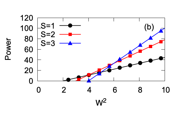
Figure 1: The power of the VA solution, in the case of $g=0$ (no quintic nonlinearity), vs. the pump’s squared width, as given by Eq. (24), which neglects weak effects of the pump and loss (small $f_{0}$ and $\alpha$), for the self-focusing ($\sigma=+1$) in (a) and defocusing ($\sigma=-1$) in (b) signs of the cubic term. The black curve with circles, the red one with squares, and the blue one with triangles pertain to vorticities $S=1$, $2$, and $3$, respectively.

In the limit of the dominant quintic nonlinearity, i.e., $g\rightarrow\pm\infty$, opposite to the pure cubic model considered above, the asymptotic solution of Eq. (19) is

$$\left(U_{0}^{2}\right)_{\mathrm{VA}}^{(g\rightarrow\pm\infty)}\approx 2^{S}\sqrt{3^{3S+1}\frac{S!}{(3S)!}}W^{-2S}$$ (26)

(in which the large coefficient $g$ cancels out), the respective expression for power (15) being

$$P_{\mathrm{VA}}^{(g\rightarrow\pm\infty)}=\frac{3^{(3S+1)/2}\pi\left(S!\right)^{3/2}}{2\sqrt{(3S)!}}W^{2},$$ (27)

cf. Eqs. (23) and (24).

In the following section, we report results of numerical solution of Eq. (1), comparing them to solutions of the full system of the VA equations (18) and (19), which include effects of the pump and loss terms.

III Numerical results

Simulations of Eq. (1) were conducted by means of the split-step pseudo-spectral algorithm. The solution procedure started from the zero input, and was running until convergence to an apparently stable stationary profile (if this outcome of the evolution was possible). This profile was then compared to its VA counterpart, produced by a numerical solution of Eqs. (18) and (19) with the same values of parameters $\alpha$, $\sigma=\pm 1$, $g$, and $f_{0}$, $W$, $S$ (see Eq. (2)). The results are presented below by varying, severally, loss $\alpha$, vorticity $S$, the pump’s width $W$ and strength $f_{0}$, and, eventually, the quintic coefficient $g$. The findings are eventually summarized in the form of stability charts plotted in Fig. 12.

III.1 Variation of the loss parameter $\alpha$

In Fig. 2(a) we display the cross-section (drawn through $y=0$) of the variational and numerical solutions for the stable vortex solitons obtained with $\alpha=0.5$, $1.0$, and $2.0$, while the other parameter are fixed as $\sigma=+1$ (the self-focusing cubic nonlinearity), $g=0$, $f_{0}=1$, $W=2$, and $S=1$. The accuracy of the VA-predicted solutions presented in Fig. 2(a) is characterized by the relative power difference from their numerically found counterparts, which is $5.1\%$, $3.1\%$, and $0.5\%$ for

$$\alpha=0.5,1.0,\mathrm{~{}}2.0,$$ (28)

respectively. Thus, the VA accuracy improves with the increase of $\alpha$.

Similar results for the self-defocusing nonlinearity, $\sigma=-1$, are presented in Fig. 2(b), which shows an essentially larger discrepancy between the VA and numerical solutions, viz., $18.9\%$, $17.4\%$, and $3.4\%$ for the same set (28) of values of the loss parameter, other coefficients being the same as in Fig. 2(a). The larger discrepancy is explained by the fact that localized (bright-soliton) modes are not naturally maintained by the self-defocusing, hence the ansatz (14), which is natural for the self-trapped solitons in the case of the self-focusing, is not accurate enough for $\sigma=-1$. In the same vein, it is natural that, in the latter case, the discrepancy is more salient for stronger nonlinearity, i.e., smaller $\alpha$, which makes the respective amplitude higher.

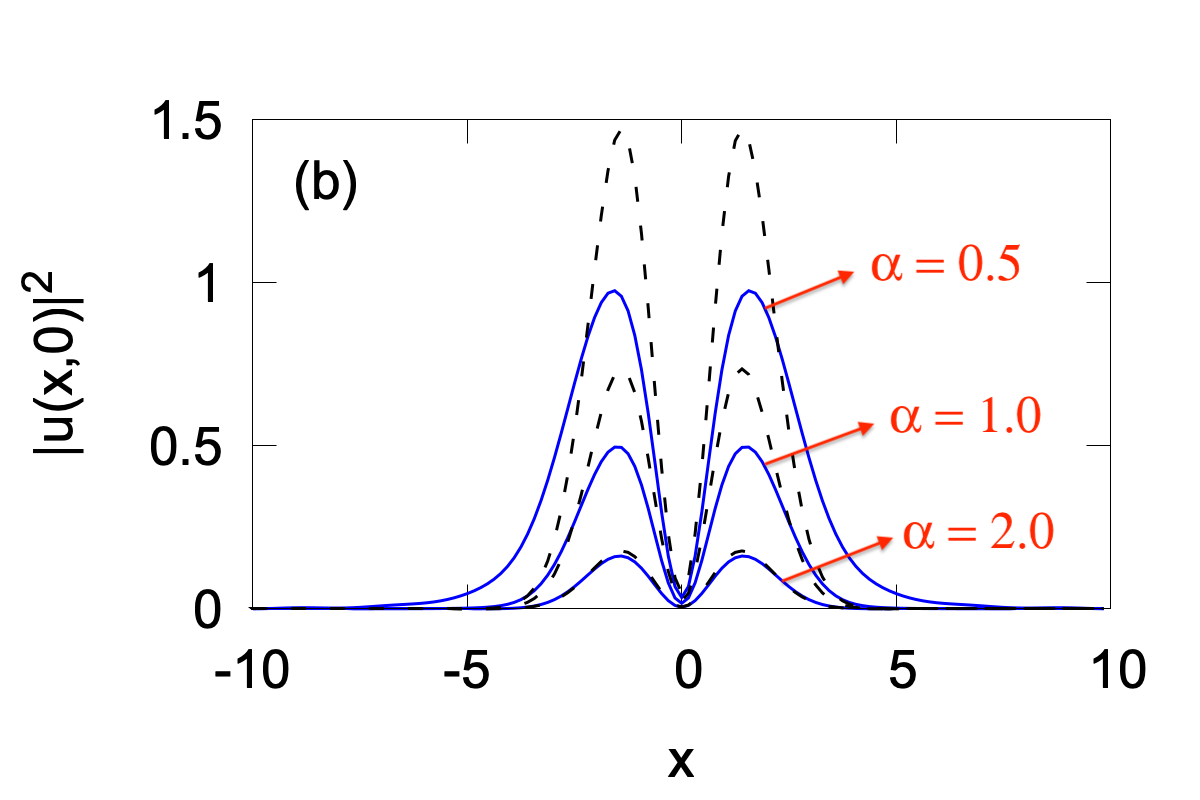
Figure 2: The comparison between cross sections (drawn through $y=0$) of the VA solutions and their numerically found counterparts (dashed black and solid blue lines, respectively) for different values of the loss parameter $\alpha$ in Eq. (1), taken from set (28). Panels (a) and (b) pertain to the self-focusing ($\sigma=+1$) and defocusing ($\sigma=-1$) signs of the cubic nonlinearity, respectively. The other parameters in Eqs. (1) and ( 2) are fixed as $g=0$, $\eta=1$, $f_{0}=1$, $W=2$, and $S=1$.

There is a critical value of $\alpha$ below which the vortex solitons are unstable. As an example, Fig. 3 shows the VA-predicted and numerically produced solutions for $\alpha=0.2$ and $\sigma=+1$ (the self-focusing nonlinearity). The observed picture may be understood as a result of the above-mentioned azimuthal MI which breaks the axial symmetry of the vortex soliton. More examples of the instability of this type are displayed below. For the values of other parameters fixed as in Fig. 3, the instability boundary is $\alpha_{\mathrm{crit}}\approx 0.35$. The stabilizing effect of the loss at $\alpha>\alpha_{\mathrm{crit}}$ is a natural feature. On the other hand, the increase of $\alpha$ leads to decrease of the soliton’s amplitude, as seen in Fig. 2.

In the case of the self-defocusing ($\sigma=-1$), all the numerically found vortex modes are stable, at least, at $\alpha\geq 0.1$, although the discrepancy in the values of the power between these solutions and their VA counterparts is very large at small $\alpha$, exceeding $75\%$ at $\alpha=0.1$. As mentioned above, the growing discrepancy is explained by the increase of the soliton’s amplitude with the decrease of $\alpha$. At still smaller values of $\alpha$, the relaxation of the evolving numerical solution toward the stationary state is very slow, which makes it difficult to identify the stability.

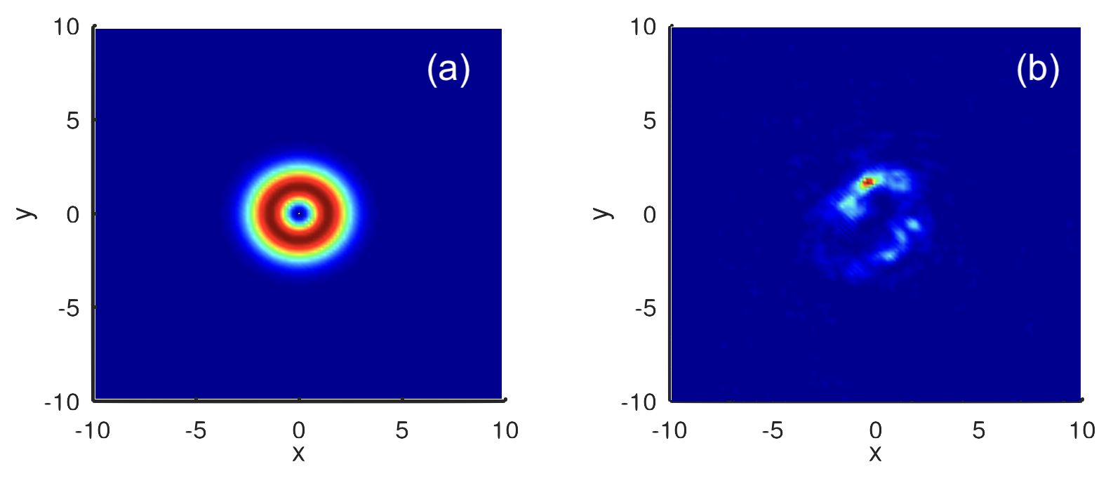
Figure 3: Profiles of $|u|^{2}$ produced by VA (a) and numerical solution at $t=100$ (b) in the case of the self-focusing ($\sigma=+1$) for $\alpha=0.2$. Other parameter are the same as in Fig. 2(a).

III.2 Variation of the pump’s vorticity $S$

To analyze effects of the winding number (vorticity) $S$, we here fix $g=0$ (the pure cubic nonlinearity) and set $\alpha=1$, $f_{0}=1$, $W=2$ in Eqs. (1) and (2). In the self-focusing case ($\sigma=+1$), the numerically produced solutions are stable for $S=1$ and $2$, and unstable for $S\geq 3$. In the former case, the power difference between the VA and numerical solutions is $3.1\%$ and $4.9\%$ for $S=1$ and $2$, respectively, i.e., the VA remains a relatively accurate approximation in this case.

In the self-defocusing case ($\sigma=-1$), considering the same values of the other parameters as used above, the numerical solution produces stable vortex solitons at least until $S=5$. For the same reason as mentioned above, the accuracy of VA is much lower for $\sigma=-1$ than for the self-focusing case ($\sigma=+1$), with the respective discrepancies in the power values being $17.4\%$, $6.7\%$, $24.1\%$, $29.0\%$, and $29.6\%$ for $S=1$, $2$, $3$, $4$, and $5$, respectively.

For the cogent verification of the stability of the localized vortices in the case of the self-defocusing, we have also checked it for smallest value of the loss parameter considered in this work, viz., $\alpha=0.1$, again for $S=1$, $2$, $3$, $4$, and $5$, and the above-mentioned values of the other coefficients, i.e., $f_{0}=1$ and $W=2$. Naturally, the discrepancy between the VA and numerical findings is still higher in this case, being $75\%$, $72.5\%$, $65.7\%$, $55.2\%$, and $41.1\%$ for $S=1$, $2$, $3$, $4$, and $5$, respectively. The result is illustrated by Fig. 4 for a relatively large vorticity, $S=4$. In particular, the pattern of $|u(x,y)|^{2}$ and the corresponding cross section, displayed in Figs. 4(b) and (c), respectively, exhibit the established vortex structure and background “garbage" produced by the evolution.

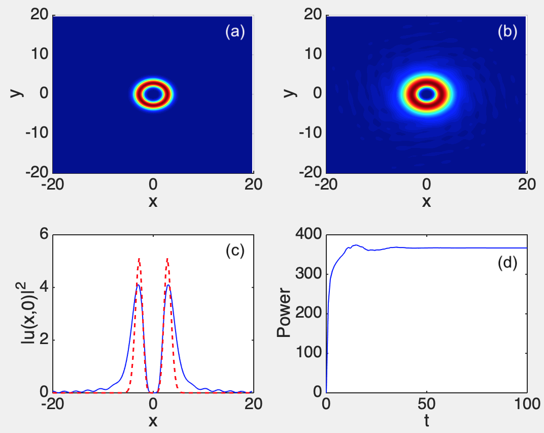
Figure 4: (a) The VA-predicted pattern and (b) the corresponding result of the direct simulation of Eq. (1) with $\sigma=-1$ and $g=0$ (cubic self-defocusing) at $t=100$, initiated by the zero input at $t=0$, for $\alpha=0.1$, $f_{0}=1$, $W=2$, and vorticity $S=4$ in the pump term (2). (c) The respective cross sections drawn through $y=0$. (d) The evolution of the total power $P$ (see Eq. (3) of the numerical solution in the course of the simulation.

III.3 Variation of the pump’s width $W$

To address the effects of the variation of parameter $W$ in Eq. (2), we here fix $g=0$, $\alpha=1$, $f_{0}=1$, and $S=1$. In Fig. 5(a), the power of the VA-predicted and numerically found stable vortex-soliton solutions is plotted as a function of $W$ for both the self-focusing and defocusing cases, i.e., $\sigma=+1$ and $\sigma=-1$, respectively. In the former case, the azimuthal MI sets in at $W\geq 2.7$, see an example in Fig. 5(b) for $W=2.75$.

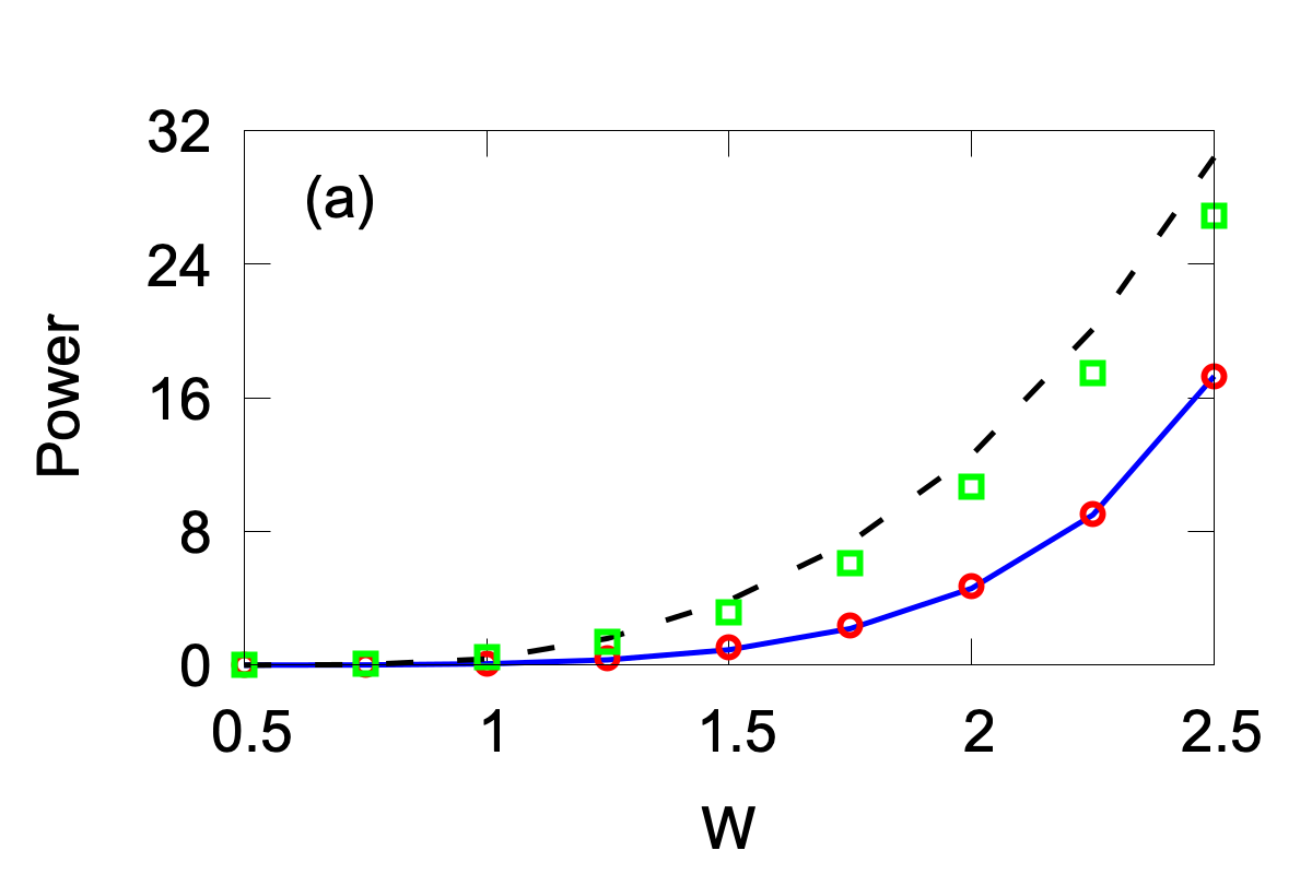
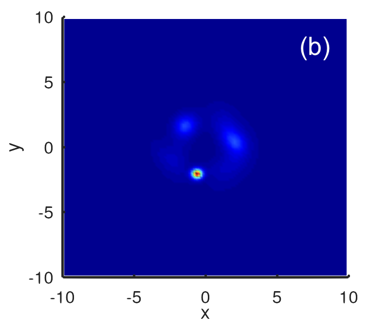
Figure 5: (a) The power of the VA-predicted vortex-soliton solutions (solid blue and dashed black lines, pertaining to the self-focusing, $\sigma=+1$, and self-defocusing, $\sigma=-1$, cubic nonlinearitry, respectively) and their numerically found counterparts (red circles and green squares pertaining to the self-focusing and self-defocusing nonlinearitry, respectively) vs. the pump’s width $W$. Other parameters are $g=0$, $\alpha=1$, $f_{0}=1$, and $S=1$. (b) The profile produced, at $t=100$, by the numerically generated unstable solution in the case of the self-focusing, $\sigma=+1$, with $W=2.75$.

In the self-focusing case, $\sigma=+1$, the azimuthal MI for the solitons with higher vorticities, $S=2$, $3$, $4$, or $5$, sets in at $W\geq 2.1$, $1.7$, $1.6$, and $1.4$, respectively. In the self-defocusing case, no existence/stability boundary was found for the vortex modes with $S=1$, $S=2$, and $S=3$ (at least, up to $W=5$). At higher values of the vorticity, the localized vortices do not exist, in the defocusing case, at $W>3.5$ and $W>2.5$, for $S=4$, and $S=5$, respectively.

III.4 Variation of the pump’s strength $f_{0}$

Effects of the variation of $f_{0}$ are reported here, fixing other parameters as $g=0$, $\alpha=1$, and $W=2$. In the case of the cubic self-focusing, $\sigma=+1$, the vortex soliton with $S=1$ are subject to MI at $f_{0}\geq 1.6$. As a typical example, in Fig. 6 we display the VA-predicted solution alongside the result of the numerical simulations for $f_{0}=1.7$. For higher vorticities, $S=2$, $3$, $4$, and $5$, the azimuthal instability sets in at $f_{0}\geq 1.1$, $0.6$, $0.3$, and $0.08$, respectively. Naturally, the narrow vortex rings with large values of $S$ are much more vulnerable to the quasi-one-dimensional azimuthal MI.

The power of the vortex solitons with $S=1$ and $2$, as produced by the VA and numerical solution, is plotted vs. the pump amplitude $f_{0}$ in Fig. 7(a). As an example, Fig. 7(b) showcases an example of the cross-section profile of the vortex soliton with $S=2$, demonstrating the reliability of the VA prediction. In the range of $f_{0}\leq 1$, the highest relative difference in the power between the numerical and variational solutions cases is $5.5\%$ and $7.5\%$ for $S=1$ and $S=2$, respectively.

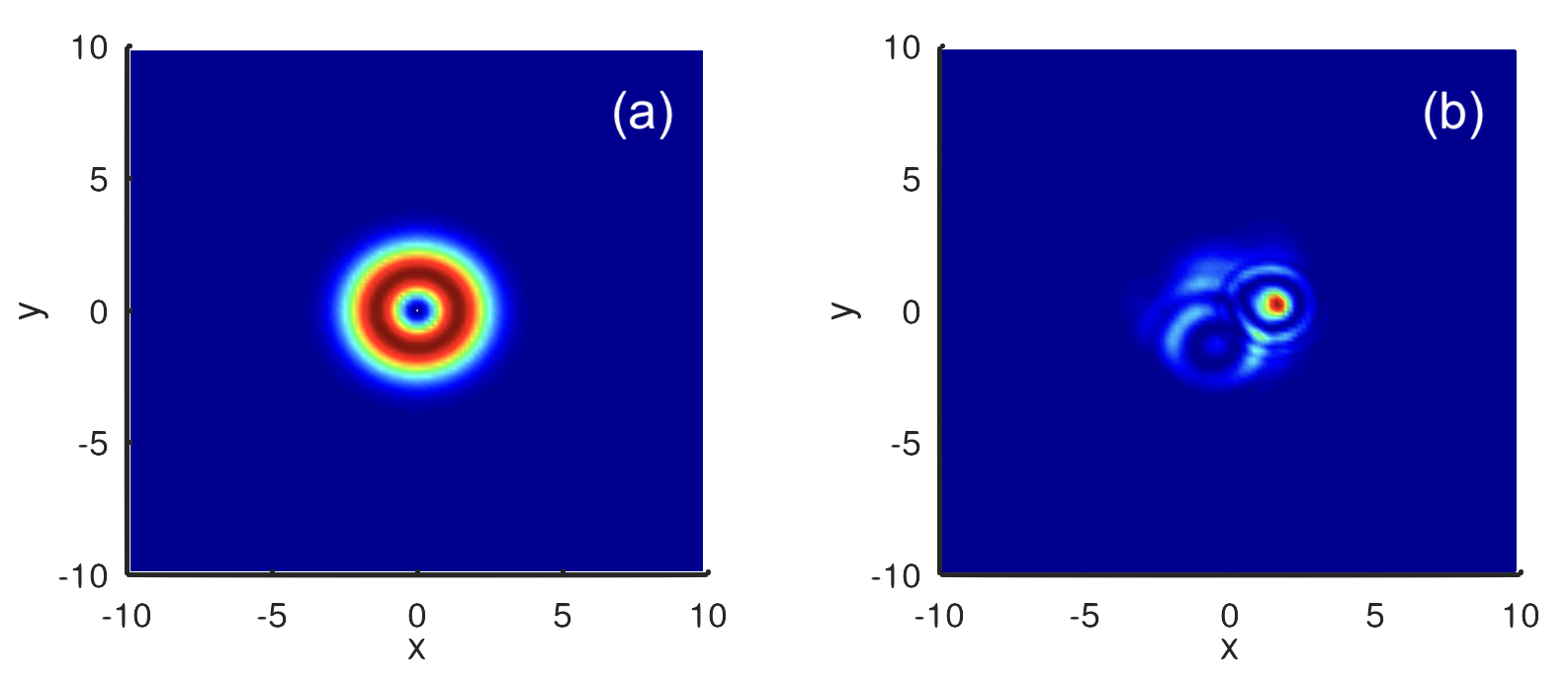
Figure 6: (a) The VA-predicted profile of $|u|^{2}$ in the self-focusing case, with parameters $g=0$, $\sigma=+1$, $\alpha=1$, $f_{0}=1.7$, $W=2$, and $S=1$. (b) The unstable solution, produced, at $t=100$, by the simulations of Eq. (1) for the same parameters.

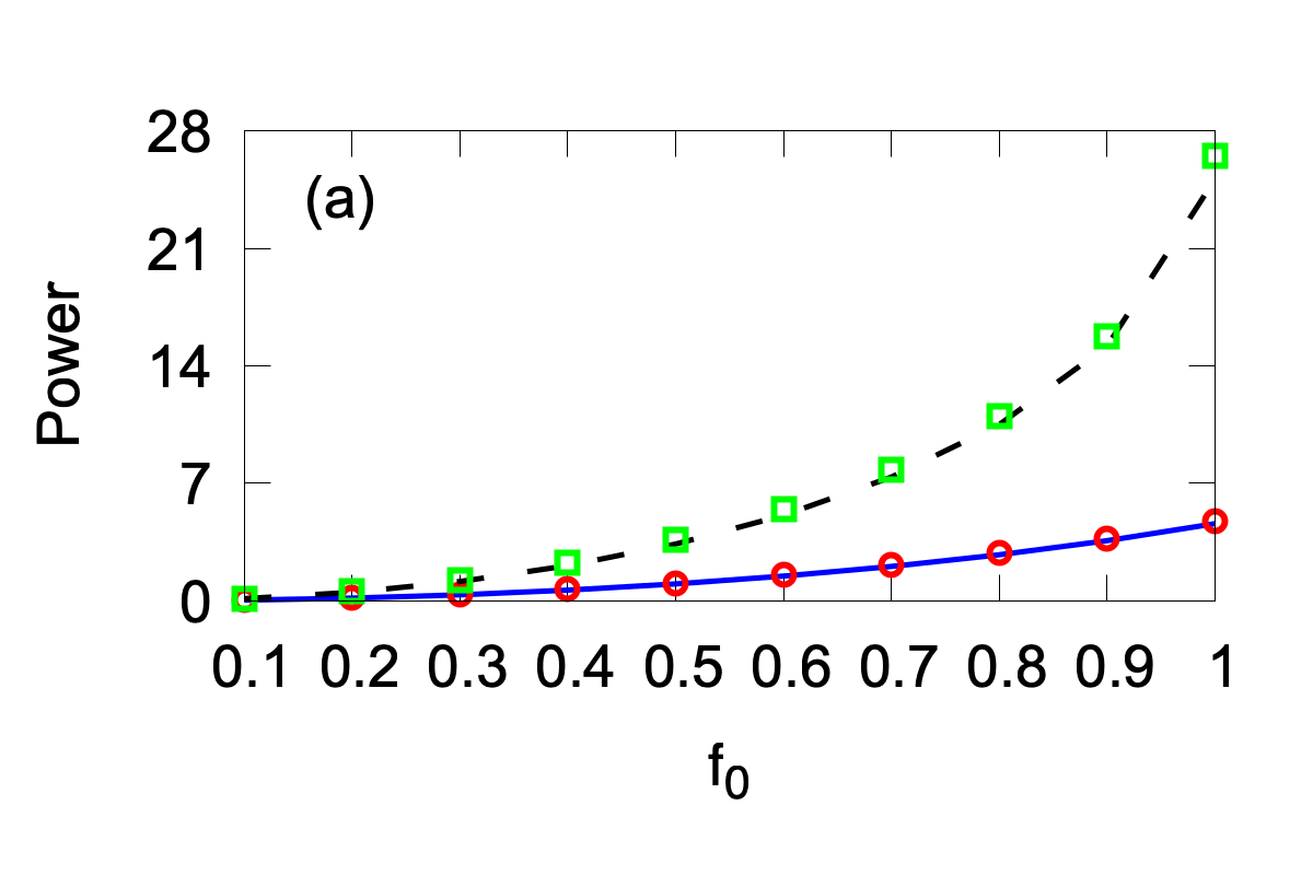
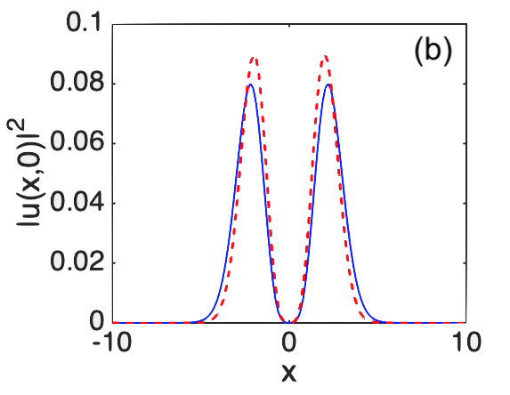
Figure 7: (a) The power versus $f_{0}$ for the confined vortex modes in the self-focusing case ($\sigma=+1$). The VA solutions for $S=1$ and $2$ are shown by solid blue and dashed black lines, respectively. The corresponding numerical solutions are represented by red circles and green squares, respectively. Recall that the numerical solutions are stable, in this case, at $f_{0}<1.6$ and $f_{0}<1.1$, for $S=1$ and $2$, respectively. (b) The VA-predicted and numerically obtained (the dashed red and solid blue lines, respectively) profiles of the stable solution with $S=2$ and $f_{0}=0.4$, drawn as cross sections through $y=0$ . The other parameters are $g=0$, $\sigma=+1$, $\alpha=1$, $W=2$.

It is relevant to mention that the “traditional” azimuthal instability of vortex-ring solitons with winding number $S$ demonstrates fission of the original axially symmetric shape into a set consisting of a large number $N\geq S$ of symmetrically placed localized fragments [40, 2], while the above examples, displayed in Figs. 3(b), 5(b), and 6(b), demonstrate the appearance of a single bright fragment and a “garbage cloud” distributed along the original ring. At larger values of $f_{0}$, our simulations produce examples of the “clean” fragmentation, viz., with $N=4$ produced by the unstable vortex rings with $S=1$ in Fig. 8(a), $N=5$ produced by $S=2$ and $3$ in (b) and (d), $N=7$ by $S=2$ and $3$ in (c) and (e), and $N=8$ by $S=3$ in (f). These outcomes of the instability development are observed at the same evolution time $t=100$ as in Figs. 3(b), 5(b), and 6(b). The gradual increase of the number of the fragments on  $S$ is explained by the dependence of the azimuthal index of the fastest growing eigenmode of the breaking instability on the underlying winding number $S$, which is a generic property of vortex solitons [40, 2].

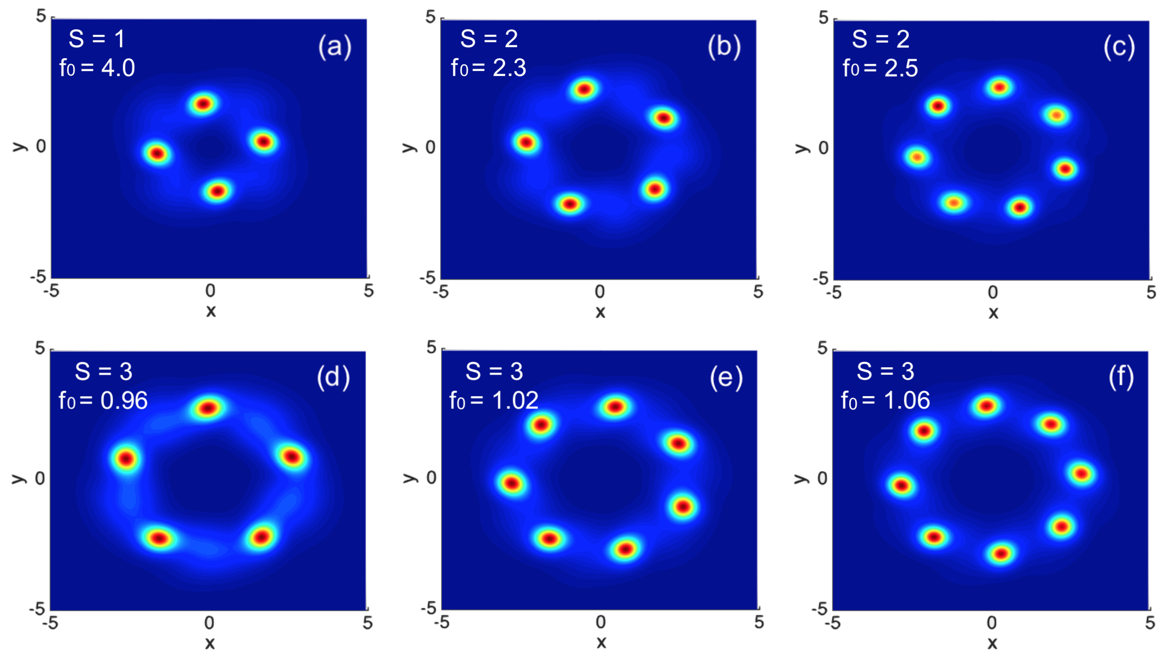
Figure 8: Examples of the fission of unstable vortex-ring solitons produced by simulations of the LL equation (1) with $\sigma=+1$ (cubic self-focusing), $g=0$ (no quintic nonlinearity), $\alpha=2$, $W=2$, and $\eta=1$. Each plot displays the result of the numerical simulations at time $t=100$. Values of the initial vorticity and pump’s strength are indicated in panels.

In self-defocusing case, $\sigma=-1$, a summary of the results produced by the VA and numerical solution for the stable vortex solitons with $S=1$ and $2$, in the form of the dependence of their power on $f_{0}$, is produced in Fig. 9(a) (cf. Fig. 7(a) for $\sigma=+1$). Naturally, the VA-numerical discrepancy increases with the growth of the pump’s strength, $f_{0}$, see an example in Fig. 9(b). Unlike the case of $\sigma=+1$, in the case of the self-defocusing the vortex modes with $S\leq 5$ remain stable, at least, up to $f_{0}=5$ (here, we do not consider the case of $S>5$).

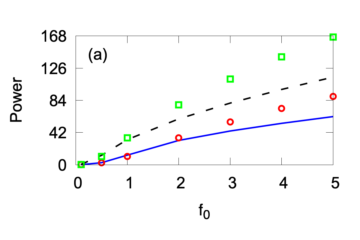
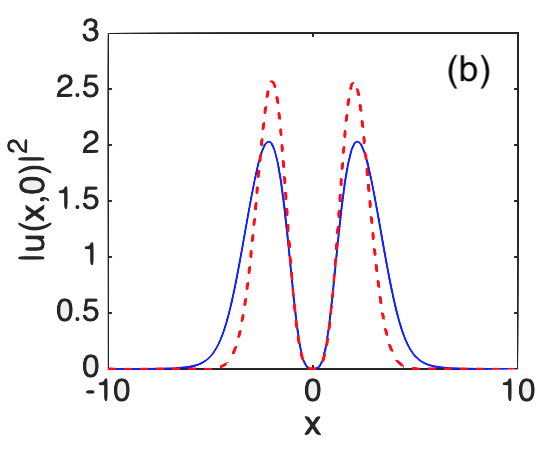
Figure 9: (a) The power versus $f_{0}$ for the vortex modes in the self-defocusing case ($\sigma=-1$). The VA solutions for $S=1$ and $2$ are shown by solid blue and dashed black lines, respectively. The corresponding numerical solutions are presented by red circles and green squares, respectively. (b) The VA-predicted and numerically obtained (the dashed red and solid blue lines, respectively) profiles of the solution with $S=2$ and $f_{0}=2$, drawn as the cross sections through $y=0$ . The other parameters are $g=0$, $\sigma=-1$, $\alpha=1$, $W=2$.

III.5 Influence of the quintic coefficient $g$

In the above analysis, the quintic term was dropped in the LL equation (1), setting $g=0$. To examine the impact of this term, we first address the case shown above in Fig. 3, which demonstrated that the vortex soliton with $S=1$, as a solution to Eqs. (1) and (2) with $g=0$, $\sigma=+1$ and $f_{0}=1$, $W=2$, was unstable if the loss parameter fell below the critical value, $\alpha=0.35$. We have found that, adding to Eq. (1) the quintic term with either $g=-1$ or $g=+1$ (the self-focusing or defocusing quintic nonlinearity, respectively) leads to the stabilization of the vortex mode displayed in Fig. 3, which was unstable in the absence of the quintic term. The stabilization of the soliton by the quintic self-defocusing is a natural fact. More surprising is the possibility to provide the stabilization by the self-focusing quintic nonlinearity because, in most cases, the inclusion of such a term gives rise to the supercritical collapse in 2D, making all solitons strongly unstable [40, 2]. However, it is concluded from the stability charts displayed below in Fig. 12 that the stabilizing effect of the quintic self-focusing occurs only at moderately small powers, for which the the quintic term is not a clearly dominant one. In the general case, solitons stability regions naturally shrink in Figs. 12 under the action of the quintic self-focusing quintic term, with $g<0$.

In the presence of the quintic term, the comparison of the numerically found stabilized vortex-soliton profiles with their VA counterparts, whose parameters are produced by a numerical solution of Eqs. (18) and (19), is presented in Fig. 10. Similar to the results for the LL equation with the cubic-only nonlinearity, the VA is essentially more accurate in the case of the self-focusing sign of the quintic term ($g<0$) than in the opposite case, $g>0$. In particular, in the case shown in Fig. 10, the power-measured discrepancy for $g=-1$ and $+1$ is, respectively, $4\%$ and $64\%$. An explanation for this observation is provided by the fact that the soliton’s amplitude is much higher in the latter case.

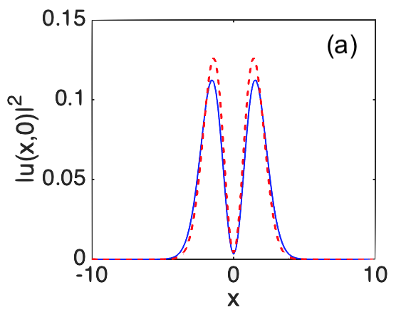
Figure 10: Cross-section profiles (drawn through $y=0$) for stable vortex solitns with $S=1$, produced by Eq. (1) with the quintic self-focusing, $g=-1$ (a) or defocusing, $g=+1$ (b) term. In both cases, the cubic self-focusing cubic term, with $\sigma=+1$, is present. The numerically found profiles and their VA-produced counterparts are displayed, respectively, by the solid blue and dashed lines. Other parameter are $\alpha=0.2$, $\eta=1$, and $f_{0}=1$, $W=2$.

Another noteworthy finding is the stabilization of higher-vorticity solitons by the quintic term. For instance, it was shown above that, for parameters $\alpha=1$, $\eta=1$, $f_{0}=1$, $W=2$, and $\sigma=+1$ (the cubic self-focusing) all vortex solitons with $S\geq 3$, produced by Eq. (1), were unstable. Now, we demonstrate that the soliton with $S=3$ is stabilized by adding the self-defocusing quintic term with a small coefficient, just $g=0.1$, see Fig. 11(b). As a counter-intuitive effect, the stabilization of the same soliton by the self-focusing quintic term is possible too, but the necessary coefficient is large, $g=-6$, see Fig. 11(a) (recall that $g=-1$ is sufficient for the stabilization of the vortex soliton with $S=1$ and $\alpha=0.2$ in Fig. 10(a)). Nevertheless, similar to what is said above, the set of Figs. 12(c,f,i) demonstrates the natural shrinkage of the stability area under the action of the quintic self-focusing. For the stabilized vortex modes shown in Fig. 11(a), in the case when both the cubic and quintic terms are self-focusing, the relative power-measured discrepancy between the numerical and VA-predicted solutions is very small, $\approx 0.7\%$, while in the presence of the weak quintic self-defocusing in Fig. 11(b) the discrepancy is $6.6\%$.

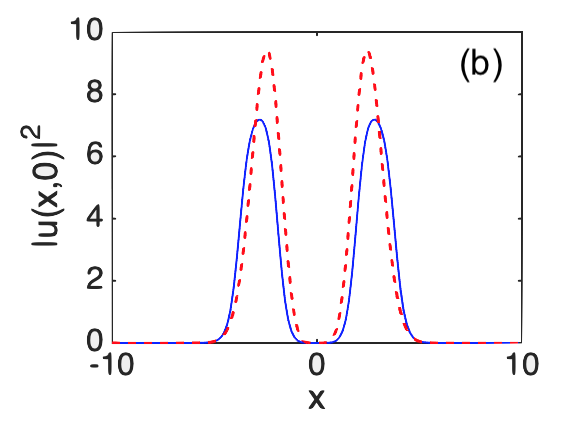
Figure 11: Cross-section profiles (drawn through $y=0$) of vortex solitons with $S=3$, stabilized by the self-focusing (a) or defocusing (b) quintic tterm in Eq. (1), with the respective coefficient $g=-6$ or $g=0.1$, other parameters being $\sigma=-1$ (cubic self-focusing), $\alpha=1$, $\eta=1$, and $f_{0}=1$, $W=2$ in Eq.( 2). The numerically found solutions and their VA-predicted counterparts are plotted by the solid blue and dashed red lines, respectively.

III.6 Stability charts in the parameter space

The numerical results produced in this work are summarized in the form of stability areas plotted in Fig. 12 in the parameter plane $\left(f_{0},\alpha\right)$, for the vortex-soliton families with winding numbers $S=1$, $2$, $3$, and three values of the quintic coefficient, $g=-1$, $0$, $+1$, while the cubic term is self-focusing, $\sigma=+1$, and the width of the pump beam is fixed, $W=2$. In addition to that, stability charts corresponding to the combination of the cubic self-defocusing ($\sigma=-1$) and quintic focusing ($g=-1$), also for $S=1,2,3$, are plotted in Fig. 13.

The choice of the parameter plane $\left(f_{0},\alpha\right)$ in the stability diagrams displayed in Fig. 12 is relevant, as the strength of the pump beam, $f_{0}$, and loss coefficient, $\alpha$,are amenable to accurate adjustment in the experiment (in particular, $\alpha$ may be tuned by partially compensating the background loss of the optical cavity by a spatially uniform pump, taken separately from the confined pump beam). As seen in all panels of Figs. 12 and 13, the increase of $\alpha$ naturally provides effective stabilization of the vortex modes, while none of them may be stable at $\alpha=0$, in agreement with the known properties of vortex-soliton solutions of the 2D nonlinear Schrödinger equation with the cubic and/or cubic-quintic nonlinearity [40, 2]. The apparent destabilization of the vortices with the increase of the pump’s amplitude $f_{0}$ is explained by the ensuing enhancement of the destabilizing nonlinearity. Other natural features exhibited by Figs. 12 are the general stabilizing/destabilizing effect of the quintic self-defocusing/focusing (as discussed above), and expansion of the splitting-instability area with the increase of $S$ (the latter feature is also exhibited by Fig. 13). The latter finding is natural too, as larger $S$ makes the ring-shaped mode closer to the quasi-1D shape (see, in particular, Fig. 8), which facilitates the onset of the above-mentioned azimuthal MI (modulational instability).

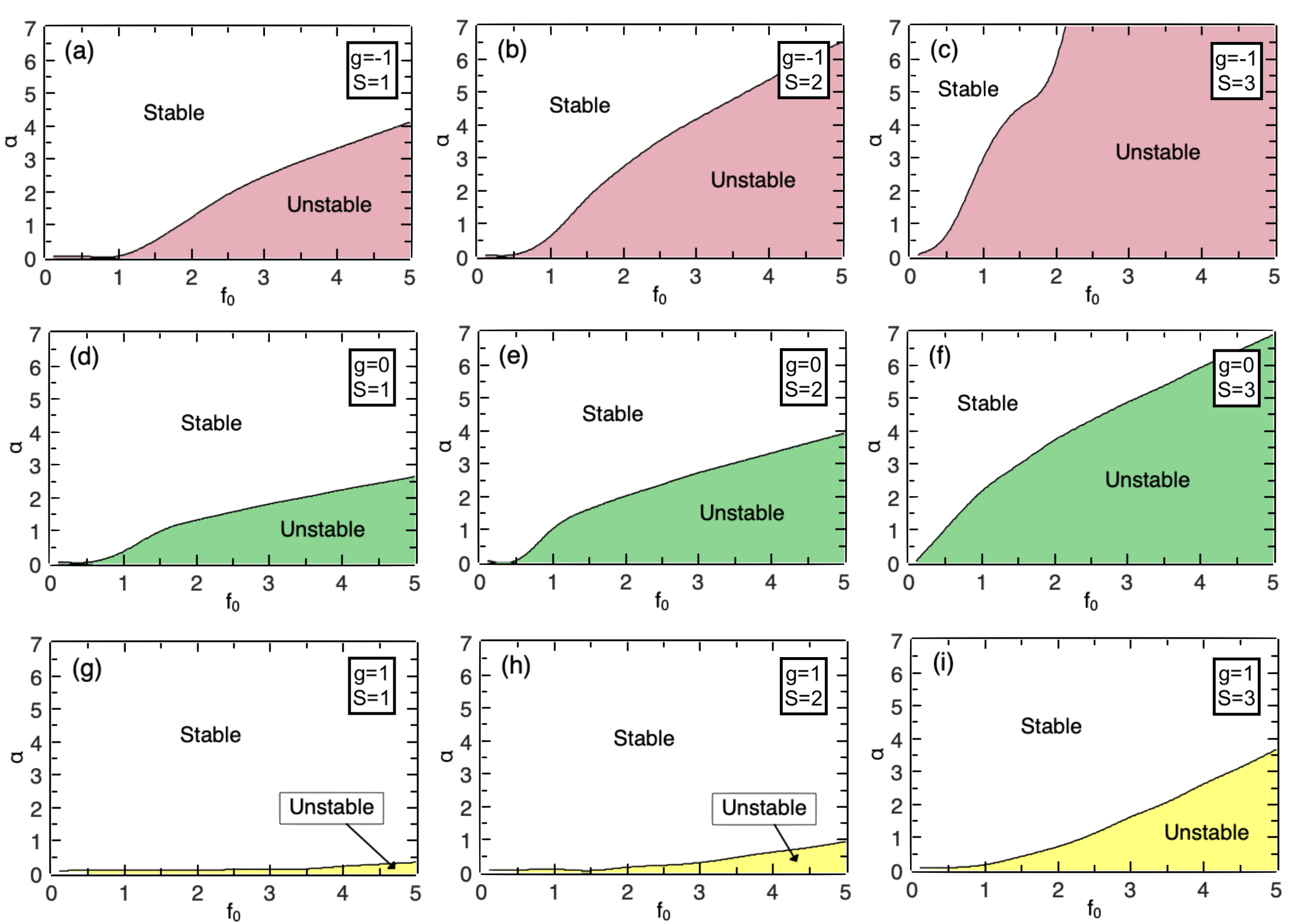
Figure 12: Stability areas for families of the vortex solitons with winding numbers $S=1$, $2,$ and $3$, in the plain of the loss coefficient ($\alpha$) and amplitude of the pump beam ($f_{0}$), for three different values of the quintic coefficient, $g=-1,0,+1$ (recall that $g<0$ and $g>0$ correspond, respectively, to the self-focusing and defocusing). Other parameters of Eqs. (1) and (2) are $\sigma=+1$ (the self-focusing cubic term), $\eta=1$, and $W=2$.

Figure 13: The same as in Figs. 12(a-c), but for $\sigma=-1$ and $g=-1$ (the cubic self-defocusing and quintic focusing terms).

Thus, the inference is that the instability mode which determines the boundary of the stability areas in Figs. 12 and 13 is the breaking of the axial symmetry of the vortex rings by azimuthal perturbations, as shown above, in particular, in Figs. 3(b), 5(b), and 6(b). The destabilization through the spontaneous splitting of the rings into symmetric sets of fragments (see Fig. 8) occurs deeply inside the instability area, i.e., at larger values of $f_{0}$.

IV Conclusion

We have introduced the two-dimensional LL (Lugiato-Lefever) equation including the self-focusing or defocusing cubic or cubic-quintic nonlinearity and the confined pump with embedded vorticity (winding number), $S\leq 5$. Stable states in the form of vortex solitons (rings) for these values of $S$ are obtained, in parallel, in the semi-analytical form by means of the VA (variational approximation) and numerically, by means of systematic simulations of the LL equation starting from the zero input. The VA provides much more accurate results in the case of the self-focusing nonlinearity than for the defocusing system. Stability areas of the vortex solitons with $S=1,2,3$ are identified in the plane of experimentally relevant parameters, viz., the pump amplitude and loss coefficient, for the self-focusing and defocusing signs of the cubic and quintic terms. Stability boundaries for the vortex rings are determined by the onset of the azimuthal instability which breaks their axial symmetry. These findings suggest new possibilities for the design of tightly confined robust optical modes, such as vortex pixels.

As an extension of this work, it may be interesting to construct solutions pinned to a symmetric pair of pump beams with or without intrinsic vorticity. In this context, it is possible to consider the beam pair with identical or opposite vorticities. In the case of the self-focusing sign of the nonlinearity, one may expect onset of spontaneous breaking of the symmetry in the dual-pump configuration. Results for this setup will be reported elsewhere.

References

- [1] Y. S. Kivshar and G. Agrawal, Optical Solitons: From Fibers to Photonic Crystals (Elsevier Science, 2003).
- [2] B. A. Malomed, Multidimensional Solitons (American Institute of Physics Publishing, Melville, NY, 2022).
- [3] N. N. Rosanov, Spatial Hysteresis and Optical Patterns (Springer: Berlin, 2002).
- [4] Dissipative Optical Solitons, ed. by M. F. S. Ferreira (Springer Nature Switzerland AG, Cham, Switzerland, 2022).
- [5] P. Grelu and N. Akhmediev, Dissipative solitons for mode-locked lasers, Nature Phot. 6, 84-92 (2012).
- [6] M. X. Jiang, X. N. Wang, Q. Ouyang, and H. Zhang, Spatiotemporal chaos control with a target wave in the complex Ginzburg-Landau equation system, Phys. Rev. E 69, 56202 (2004).
- [7] L. A. Lugiato and R. Lefever, Spatial Dissipative Structures in Passive Optical Systems, Phys. Rev. Lett. 58, 2209 (1987).
- [8] M. Tlidi and K. Panajotov, Two-dimensional dissipative rogue waves due to time-delayed feedback in cavity nonlinear optics, Chaos 27, 013119 (2017).
- [9] K. Panajotov, M. G. Clerc, and M. Tlidi, Spatiotemporal chaos and two-dimensional dissipative rogue waves in Lugiato-Lefever model, Eur. Phys. J. B 71, 176 (2017).
- [10] M. Tlidi and M. Taki, Rogue waves in nonlinear optics, Adv. Opt. Photon. 14, 87-147 (2022).
- [11] Y. Sun, P. Parra-Rivas, F. Mangini, and S. Wabnitz, Multidimensional localized states in externally driven Kerr cavities with a parabolic spatiotemporal potential: a dimensional connection, arXiv:2401.15689.
- [12] G. J. de Valcárcel and K. Staliunas, Phase-bistable Kerr cavity solitons and patterns, Phys. Rev. A 87, 043802 (2013).
- [13] S. Coen, H. G. Randle, T. Sylvestre, and M. Erkintalo, Modeling of octave-spanning Kerr frequency combs using a generalized mean-field Lugiato-Lefever model, Opt. Lett. 38, 37-39 (2013).
- [14] M. R. E. Lamont, Y. Okawachi, and A. L. Gaeta, Route to stabilized ultrabroadband microresonator-based frequency combs, Opt. Lett. 38, 3478-3481 (2013).
- [15] C. Godey, I. V. Balakireva, A. Coillet, and Y. K. Chembo, Stability analysis of the spatiotemporal Lugiato-Lefever model for Kerr optical frequency combs in the anomalous and normal dispersion regimes, Phys. Rev. A 89, 063814 (2014).
- [16] V. E. Lobanov, G. Lihachev, T. J. Kippenberg, and M. L. Gorodetsky, Frequency combs and platicons in optical microresonators with normal GVD, Opt. Exp. 23, 7713-7721 (2015).
- [17] M. Karpov, H. Guo, A. Kordts, V. Brasch, M. H. P. Pfeiffer, M. Zervas, M. Geiselmann, and T. J. Kippenberg, Raman Self-Frequency Shift of Dissipative Kerr Solitons in an Optical Microresonator, Phys. Rev. Lett. 116, 103902 (2016).
- [18] F. Copie, M. Conforti, A. Kudlinski, A. Mussot, and S. Trillo, Competing Turing and Faraday Instabilities in longitudinally modulated passive resonators, Phys. Rev. Lett. 116, 143901 (2016).
- [19] P. Parra-Rivas, D. Gomila, P. Colet, and L. Gelens, Interaction of solitons and the formation of bound states in the generalized Lugiato-Lefever equation, Eur. Phys. J. D 71, 198 (2017).
- [20] M. G. Clerc, M. A. Ferré, S. Coulibaly, R. G. Rojas, and M. Tlidi, Chimera-like states in an array of coupled-waveguide resonators, Opt. Lett. 42, 2906-2909 (2017).
- [21] B. Garbin, Y. Wang, S. G. Murdoch, G.-L. Oppo, S. Coen, and M. Erkintalo, Experimental and numerical investigations of switching wave dynamics in a normally dispersive fibre ring resonator, Eur. Phys. J. D 71, 240 (2017).
- [22] Q. Li, T. C. Briles, D. A. Westly, T. E. Drake, J. R. Stone, B. R. Ilic, S. A. Diddams, S. B. Papp, and K. Srinivasan, Stably accessing octave-spanning microresonator frequency combs in the soliton regime, Optica 4, 193-203 (2017).
- [23] L. A. Lugiato, F. Prati, M. L. Gorodetsky, and T. J. Kippenberg, From the Lugiato–Lefever equation to microresonator-based soliton Kerr frequency combs, Phil. Trans. R. Soc. A. 376, 20180113 (2018).
- [24] X. Dong, C. Spiess, V. G. Bucklew, and W. H. Renninger, Chirped-pulsed Kerr solitons in the Lugiato-Lefever equation with spectral filtering, Phys. Rev. Research 3, 033252 (2021).
- [25] S.-W. Huang, J. Yang, S.-H. Yang, M. Yu, D.-L. Kwong, T. Zelevinsky, M. Jarrahi, and C. W. Wong, Globally stable microresonator Turing pattern formation for coherent high-power THz radiation on-chip, Phys. Rev. X 7, 041002 (2017).
- [26] Y. V. Kartashov, O. Alexander, and D. V. Skryabin, Multistability and coexisting soliton combs in ring resonators: the Lugiato-Lefever approach, Opt. Express 25, 11550-11555 (2017).
- [27] A. Coillet, I. Balakireva, R. Henriet, K. Saleh, L. Larger, J. M. Dudley, C. R. Menyuk, Y. K. Chembo, Azimuthal Turing patterns, bright and dark cavity solitons in Kerr combs generated with whispering-gallery-mode resonators, IEEE Photon. J. 5, 6100409-6100409 (2013).
- [28] Y. K. Chembo and C. R. Menyuk, Spatiotemporal Lugiato-Lefever formalism for Kerr-comb generation in whispering-gallery-mode resonators, Phys. Rev. A 87, 053852 (2013).
- [29] H. Taheri, A. A. Eftekhar, K. Wiesenfeld, and A. Adibi, Soliton Formation in Whispering-Gallery-Mode Resonators via Input Phase Modulation, IEEE Photon. J. 7, 2200309 (2015).
- [30] Y.-Y. Wang, M.-M. Li, G.-Q. Zhou, Y. Fan, and X.-J. Lai, Rotating vortex-like soliton in a whispering gallery mode microresonator, Eur. Phys. J. Plus 134, 161 (2019).
- [31] T. Daugey, C. Billet, J. Dudley, J.-M. Merolla, and Y. K. Chembo, Kerr optical frequency comb generation using whispering-gallery-mode resonators in the pulsed-pump regime, Phys. Rev. A 103, 023521 (2021).
- [32] Q.-H. Cao, K.-L. Geng, B-W. Zhu, Y.-Y. Wang, and C.-Q. Dai, Scalar vortex solitons and vector dipole solitons in whispering gallery mode optical microresonators, Chaos, Sol. & Fract. 166, 112895 (2023).
- [33] W. B. Cardoso, L. Salasnich, and B. A. Malomed, Localized solutions of Lugiato-Lefever equations with focused pump, Sci. Rep. 7, 16876 (2017).
- [34] W. B. Cardoso, L. Salasnich, and B. A. Malomed, Zero-dimensional limit of the two-dimensional Lugiato-Lefever equation. Eur. Phys. J. D 71, 112 (2017).
- [35] M. Quiroga-Teixeiro and H. Michinel, Stable azimuthal stationary state in quintic nonlinear optical media, J. Opt. Soc. Am. B 14, 2004-2009 (1997).
- [36] G. Boudebs, S. Cherukulappurath, H. Leblond, J. Troles, F. Smektala, and F. Sanchez, Experimental and theoretical study of higher-order nonlinearities in chalcogenide glasses, Opt. Commun. 219, 427-432 (2003).
- [37] A. S. Reyna and C. B. de Araújo, High-order optical nonlinearities in plasmonic nanocomposites – a review, Adv. Opt. Phot. 9, 720-774 (2017).
- [38] D. L. Andrews, symmetry and quantum features in optical vortices, Symmetry 13, 1368 (2021).
- [39] A. Ramaniuk, N. V. Hung, M. Giersig, K. Kempa, V. V. Konotop, and M. Trippenbach, Vortex creation without stirring in coupled ring resonators with gain and loss, Symmetry 10, 195 (2018).
- [40] B. A. Malomed, (INVITED) Vortex solitons: Old results and new perspectives, Physica D 399, 108-137 (2019).
- [41] R. K. Bullough, A. P. Fordy, and S. V. Manakov, Adiabatic invariants theory of near-integrable systems with damping, Phys. Lett. A 91, 98-100 (1982).