Semi-Supervised Unconstrained Head Pose Estimation in the Wild

Abstract

Existing head pose estimation datasets are either composed of numerous samples by non-realistic synthesis or lab collection, or limited images by labor-intensive annotating. This makes deep supervised learning based solutions compromised due to the reliance on generous labeled data. To alleviate it, we propose the first semi-supervised unconstrained head pose estimation (SemiUHPE) method, which can leverage a large amount of unlabeled wild head images. Specifically, we follow the recent semi-supervised rotation regression, and focus on the diverse and complex head pose domain. Firstly, we claim that the aspect-ratio invariant cropping of heads is superior to the previous landmark-based affine alignment, which does not fit unlabeled natural heads or practical applications where landmarks are often unavailable. Then, instead of using an empirically fixed threshold to filter out pseudo labels, we propose the dynamic entropy-based filtering by updating thresholds for adaptively removing unlabeled outliers. Moreover, we revisit the design of weak-strong augmentations, and further exploit its superiority by devising two novel head-oriented strong augmentations named pose-irrelevant cut-occlusion and pose-altering rotation consistency. Extensive experiments show that SemiUHPE can surpass SOTAs with remarkable improvements on public benchmarks under both front-range and full-range. Our code is released in https://github.com/hnuzhy/SemiUHPE.

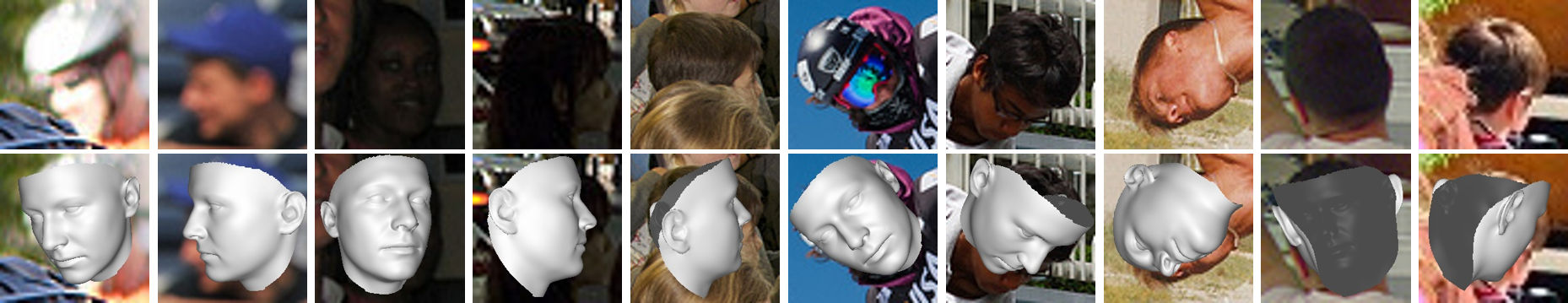
Figure 1: Our unconstrained head pose estimation results on wild challenging heads (e.g., heavy blur, extreme illumination, severe occlusion, atypical pose, and invisible face).

1 Introduction

Human head pose estimation (HPE) from a single RGB image in the wild is a long-standing yet still challenging problem [36, 1]. It has numerous applications such as driver monitoring [37], classroom observation [2], and eye-gaze proxy [3, 40]. Meanwhile, HPE can also serve as a crucial auxiliary to facilitate other face or head related multi-tasks (e.g., landmark localization [43, 56], face alignment [76, 18, 51, 4] and face shape reconstruction [66, 34]).

In the era of deep supervised learning, many HPE methods [46, 64, 75, 20] need a large amount of labeled data to train. However, existing HPE datasets such as 300W-LP [76], BIWI [15] and DAD-3DHeads [34] have their incompatible limitations for real applications. They are either artificially collected or synthesized [76, 15, 17, 27] so that having huge domain gaps and scarce diversities compared to natural heads, or manually annotated by experts [34, 55] at a significant time and economic cost with a small scale. Some samples are shown in Fig. 2. To this end, we turn to semi-supervised learning (SSL) [50, 5, 49, 58], and propose a semi-supervised unconstrained head pose estimation (SemiUHPE) method, that can leverage extensive easier obtainable yet unlabeled wild heads [31, 63, 48] in addition to partially labeled data to improve performance and generalization. Our method can not only avoid the laborious annotation of 3D head pose on 2D images which itself is ill-posed, but also greatly promote the estimation accuracy of challenging cases in real environments.

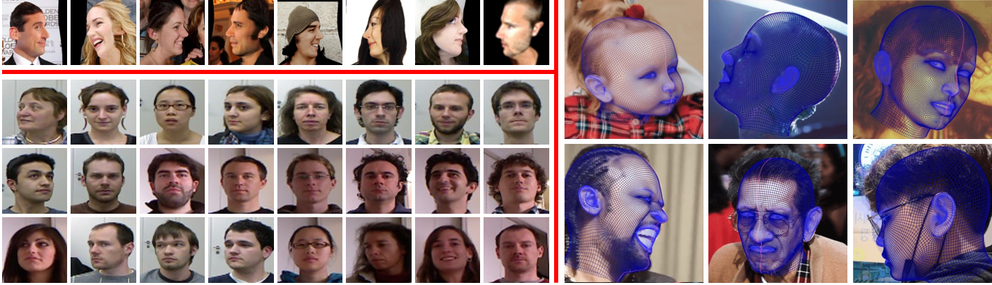
Figure 2: Examples of front-range datasets 300W-LP (left-up) having synthesized profile faces with many artifacts and BIWI (left-down) collected in lab with only 24 sequences, and full-range DAD-3DHeads (right) with head mesh labels on 2D images.

Specifically, our work is inspired by the recent proposed semi-supervised rotation regression method FisherMatch [65] of generic objects. FisherMatch inherits two widely used paradigms in semi-supervised classification: the Mean-Teacher framework [50] and the pseudo label filtering devised by FixMatch [49]. Its main contribution is to use the entropy of prediction with the matrix Fisher distribution [29, 35] as a measure for filtering pseudo labels, which resembles the classification confidence and enables it to handle semi-supervised rotation regression similar to FixMatch. Following this, we focus on the head pose estimation, which is a typical case of the general object rotation regression. This is a quite non-trivial problem that cannot be well-solved by FisherMatch due to many less-touched challenging heads. Beyond that, we aim to address unconstrained head pose estimation (UHPE) of omnidirectionality, including heads with common front-range angles and face-invisible back-range angles.

To tackle the semi-supervised UHPE task, we mainly propose the following three strategies for improvement: (1) Aspect-Ratio Invariant Cropping. We observe that previous methods [46, 64, 75, 20] require aligned faces as inputs, which relies on pre-annotated landmarks. However, this does not apply to our task as back-range heads cannot be aligned and unlabeled data has no landmark labels. Moreover, face alignment during training can cause the affine deformation, thereby hindering the inference on natural heads. Therefore, we recommend using the landmark-free pre-processing of head cropping to maintain aspect-ratio invariant and enhance practical generalization ability. (2) Dynamic Entropy-based Filtering. A key design of FixMatch is the confidence-based pseudo label filtering. FisherMatch develops the prediction entropy-based version for rotation regression. Although a pre-fixed threshold has been validated to be effective, dynamic thresholds also make sense. Such as the curriculum pseudo labeling [68], label grouping [39] and adaptive threshold [57]. For our task, due to the intermixing of hard and noisy samples in unlabeled wild heads, we consider that gradually updating the threshold as the training converges is a better and more general choice. (3) Head-Oriented Strong Augmentations. Another key idea of FixMatch is the weak-strong paired augmentations, which feeds the teacher model by weakly augmented unlabeled inputs to guide the student model fed by the same unlabeled yet strongly augmented inputs. Based on it, some SSL methods for detection [26], segmentation [61] and keypoints [59, 23] found that an advanced strong augmentation is quite important. Similarly, we re-examine the properties of unlabeled heads and invent two novel superior augmentations: pose-irrelevant cut-occlusion and pose-altering rotation consistency. In method section, we will provide more details of above-mentioned strategies.

In experiments, we demonstrate the effectiveness and versatility of our proposed strategies by extensive ablation studies. In addition, our method provides impressive qualitative estimation results on wild challenging heads, which is promising for downstream applications. To sum up, we have four contributions: (1) The semi-supervised unrestricted head pose estimation (SemiUHPE) for wild RGB images is proposed for the first time. (2) A well-performed framework including novel customized strategies for tackling the SemiUHPE task is proposed. (3) Benchmarks for the SemiUHPE are constructed. (4) New SOTA results are achieved under both front-range and full-range HPE settings.

2 Related Work

RGB-based Head Pose Estimation Human head pose estimation (HPE) using monocular RGB images is a widely researched field [36, 1]. Benefiting from deep CNN, data-driven supervised learning methods tend to dominate this field. Basically, we can divide them into four categories based on landmarks [25, 6, 76, 11, 7], Euler angles [46, 64, 75, 70, 16, 55, 73], vectors [21, 8, 32, 10, 4, 20, 69] or 3D Morphable Model (3DMM) [76, 18, 45, 56, 34, 24, 30]. Euler angles-based methods are essentially hindered by the gimbal lock. Vectors-based methods using representations such as unit quaternion [21], rotation vector [4] and rotation matrix [32, 20, 69] can alleviate this drawback and allow full-range predictions. The 3DMM-based methods treat HPE as a subtask with optimizing multi-tasks when doing 3D face reconstruction, which currently keep SOTA on both front-range [56, 30] and full-range [34] HPE. In this paper, we focus on full-range unconstrained HPE and choose rotation matrix as the pose representation.

Semi-Supervised Learning (SSL) The SSL aims to improve models by exploiting a small-scale labeled data and a large-scale unlabeled data. It can be categorized into pseudo-label (PL) based [42, 41, 49, 39, 57, 38] and consistency-based [28, 50, 5, 58, 68, 22]. The PL-based method iteratively selects unlabeled images into the training data by utilizing suitable thresholds to filter out uncertain samples with low-confidence. While, the consistency-based method enforces outputs or intermediate features to be consistent when the input is randomly perturbed. For example, MixMatch [5] combines consistency regularization with entropy minimization to obtain confident predictions. Based on MixMatch, SimPLE [22] proposes to exploit similar high confidence pseudo labels. FixMatch [49] integrates both pseudo label filtering and weak-to-strong augmentation consistency. FlexMatch [68], CCSSL [60] and FullMatch [9] extend FixMatch by adopting the curriculum pseudo labeling, contrastive learning and usage of all unlabeled data, respectively. We follow the empirically powerful FixMatch family [68, 60, 9, 57] to propose novel solutions for tackling HPE.

Semi-Supervised Rotation Regression This is a less-studied field compared with other popular SSL tasks such as classification and detection. For the 6D pose estimation, Self6D [54, 53] establishes self-supervision for 6D pose by enforcing visual and geometric consistencies on top of unlabeled RGB-D images. NVSM [52] builds a category-level 3D cuboid mesh for estimating pose of rigid object in a synthesis-and-matching way. Recently, based on FixMatch [49], FisherMatch [65] firstly proposes the semi-supervised rotation regression for generic objects. It can automatically learn uncertainties along with predictions by introducing the matrix Fisher distribution [29, 35] to build a probabilistic model of rotation. The entropy of this distribution has been validated to be an efficient indicator of prediction for pseudo label filtering. Essentially, the human HPE is subordinate to the rotation regression problem. MFDNet [32] also utilizes the matrix Fisher distribution to model head rotation uncertainty. We follow [65, 32] and adopt this distribution to tackle the SemiUHPE task.

3 Method

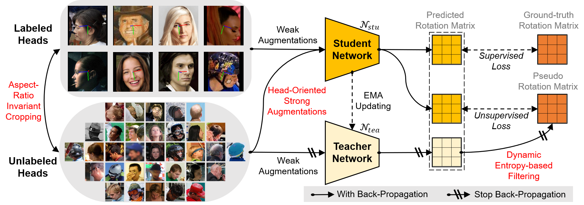
Figure 3: The illustration of our SemiUHPE. We leverage small-scale labeled heads and large-scale unlabeled wild heads to optimize the teacher-student mutual learning Mean-Teacher framework. Three customized strategies are marked with red color. We finally keep the student model which is more efficient and robust for HPE evaluation.

3.1 Problem Definition

Our SemiUHPE aims to utilize a small set of head images with pose labels $\mathcal{D}^{l}\!=\!\{(\mathbf{x}^{l}_{i},\mathbf{y}^{l}_{i})\}_{i=1}^{N_{l}}$ and fully explore a large set of unlabeled head images $\mathcal{D}^{u}\!=\!\{\mathbf{x}^{u}_{i}\}_{i=1}^{N_{u}}$. Here, $\mathbf{x}^{l}$ and $\mathbf{x}^{u}$ represent labeled and unlabeled RGB images respectively, and $\mathbf{y}^{l}_{i}$ is the ground-truth head pose label of $\mathbf{x}^{l}$ such as a rotation matrix or three Euler angles. The $N_{l}$ and $N_{u}$ are the number of labeled and unlabeled head images, respectively. Usually, the labeled set $\mathcal{D}^{l}$ contains either many accurate annotations yet non-photorealistic images (e.g. 300W-LP [76]), or laboriously hand-annotated labels but limited images (e.g. DAD-3DHeads [34]). The unlabeled set $\mathcal{D}^{u}$ has much more realistic wild heads with spontaneous expressions and diversified properties. Such as COCO [31]. For those challenging heads, we need to exploit the in-distribution valuable portion $\mathcal{D}^{u}_{id}$ that is less-explored, and avoid negative impact of the noisy out-of-distribution portion $\mathcal{D}^{u}_{ood}$.

3.2 Framework Overview

As shown in Fig. 3, we adopt the Mean-Teacher [50]. The teacher model $\mathcal{N}_{tea}$ is the exponential moving average (EMA) of the student model $\mathcal{N}_{stu}$. While, the $\mathcal{N}_{stu}$ is supervisedly trained by labeled data, and also unsupervisedly guided by pseudo labels of unlabeled data predicted by the $\mathcal{N}_{tea}$. In this way, two models are enforced by the history consistency. Then, FixMatch [49] extends it by combining weak-strong augmentations and pseudo label filtering for classification. For rotation regression, FisherMatch [65] follows FixMatch and utilizes the entropy of predicted matrix Fisher distribution as a measure for pseudo label filtering. We briefly review this probabilistic rotation distribution below.

Matrix Fisher Distribution $\mathcal{MF}(\mathbf{R};\mathbf{A})$ This is a favorable probabilistic modeling of deep rotation estimation, which has a bounded gradient [35, 32] and intrinsic advantage than its counterpart Bingham distribution [29]. Specifically, it is a distribution over $\mathcal{SO}$(3) with probability density function as:

$$\small p(\mathbf{R})=\mathcal{MF}(\mathbf{R};\mathbf{A})=\frac{1}{F(\mathbf{A})}\exp(\text{tr}(\mathbf{A}^{T}\mathbf{R}))$$ (1)

where $\mathbf{A}\!\in\!\mathbb{R}^{3\times 3}$ is an arbitrary $3\!\times\!3$ matrix and $F(\mathbf{A})$ is the normalizing constant. Then, the mode $\mathbf{R}$ and dispersion $\mathbf{S}$ of the distribution are computed as:

$$\small\mathbf{R}=\mathbf{U}\left[\begin{array}[]{ccc}1&\quad 0&\quad 0\\ 0&\quad 1&\quad 0\\ 0&\quad 0&\quad\det(\mathbf{U}\mathbf{V})\end{array}\right]\mathbf{V}^{T}$$ (2)

where $\mathbf{U}$ and $\mathbf{V}$ are from the singular value decomposition (SVD) of $\mathbf{A}\!=\!\mathbf{U}\mathbf{S}\mathbf{V}^{T}$. Each singular value $s_{i}$ in $\mathbf{S}\!=\!\text{diag}(s_{1},s_{2},s_{3})$ is sorted in descending order, and indicates the concentration strength.

Entropy-based Confidence Measure During training, the network regressor $\mathcal{N}$ takes a single RGB image $\mathbf{x}$ as input and outputs a $3\!\times\!3$ matrix $\mathbf{A}_{f}\!=\!\mathcal{N}(\mathbf{x})$. The predicted $\mathbf{A}_{f}$ is a matrix Fisher distribution $f\!\sim\!\mathcal{MF}(\mathbf{A}_{f})$. It contains a predicted rotation and the information of concentration by computing mode $\mathbf{R}_{f}$ and dispersion $\mathbf{S}_{f}$ as in Eq. 2, respectively. The entropy of this prediction, used as confidence measure of uncertainty, can be computed as:

$$\small H(f)=\log{F_{f}}-\sum\nolimits^{4}_{i=1}\left({z_{f_{i}}\frac{1}{F_{f}}\frac{\partial{F_{f}}}{\partial{z_{f_{i}}}}}\right)$$ (3)

where $F_{f}$ is constant wrt. parameter $\mathbf{Z}\!=\!\text{diag}(0,z_{1},z_{2},z_{3})$. And $\mathbf{Z}$ is a $4\!\times\!4$ diagonal matrix with $0\!\geq\!z_{1}\!\geq\!z_{2}\!\geq\!z_{3}$. The element $z_{i}$ is from the corresponding unit quaternion $\mathbf{q}\!\in\!\mathcal{S}^{3}$. Assume $\mathbf{A}_{f}\!=\!\mathbf{U}_{f}\mathbf{S}_{f}\mathbf{V}_{f}^{T}$, $\gamma$ is the standard transform from unit quaternion to rotation matrix, $\mathbf{e}_{i}$ is the $i$-th column of $\mathbf{I}_{4}$, and $\mathbf{E}_{i}\!=\!\gamma(\mathbf{e}_{i})$, then $z_{f_{i}}$ is the trace of $\mathbf{E}_{i}^{T}\mathbf{S}_{i}$. More details of the derivation are in [35, 65]. Generally, a lower entropy indicates a more peaked distribution that means less uncertainty and higher confidence.

3.3 Aspect-Ratio Invariant Cropping

For input preprocessing, we call for keeping the aspect-ratio invariant by loosely cropping head-centered images with bounding boxes and padding the out-of-plane area with zero. The reasons are two-fold. Firstly, the naive cropping-resizing may lead to scaling-related flaws [35] such as perceived orientation change. Secondly, existing HPE methods [46, 64, 75, 20] take it for grant that aligning face with landmarks will bring better results like face recognition [33, 12]. However, this often introduces severe affine deformation that disrupts the natural face. See Fig. 5 for reference. Moreover, face landmarks are not applicable to back-range or wild-collected heads. We will verify the necessity and advantages of aspect-ratio invariant cropping in experiments.

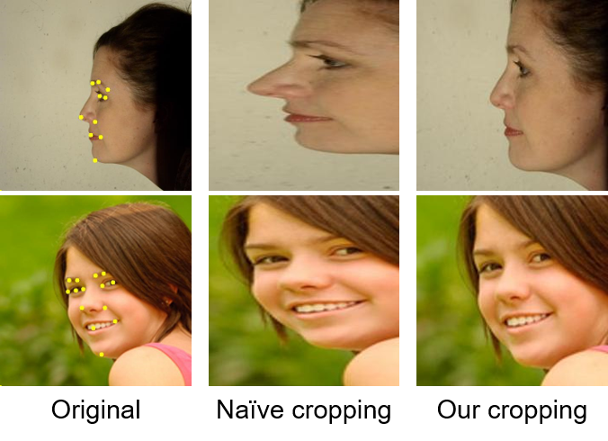
Figure 4: The illustration of how a naive cropping-resizing leads to perceived orientation and affine deformation.

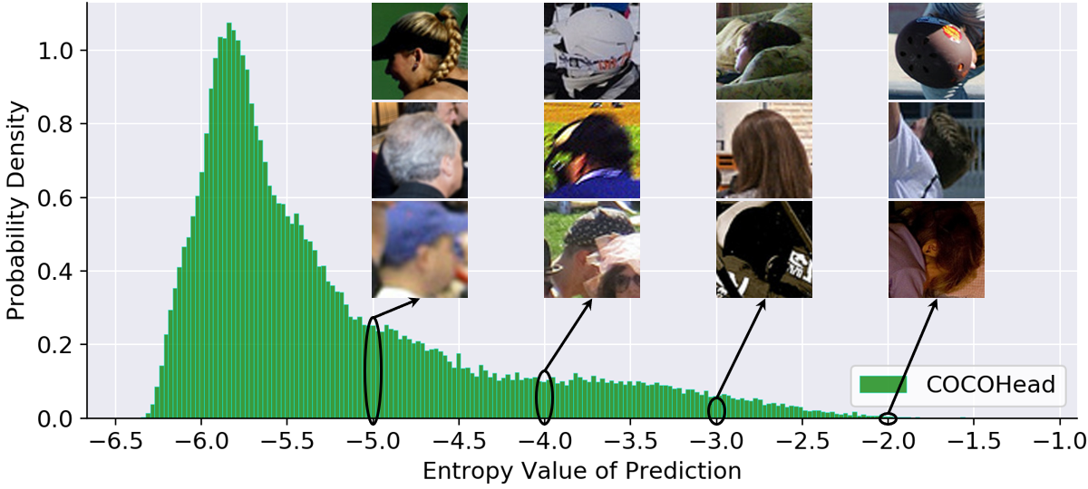
Figure 5: The illustration of prediction entropies corresponding to their head samples in the unlabeled dataset (e.g. COCOHead).

3.4 Dynamic Entropy-based Filtering

In original FisherMatch, it adopts a trivial entropy-based filtering rule on unlabeled data which keeps the prediction as a pseudo label when its entropy is lower than a pre-fixed threshold $\tau$. The obtained unsupervised loss is:

$$\small\mathcal{L}_{unsup}(\mathbf{x}^{u})=\mathds{1}_{(H(p_{tea})\leq\tau)}\mathcal{L}^{CE}(p_{tea},p_{stu})$$ (4)

where $\mathds{1}_{(\cdot)}$ is the indicator function, being 1 if the condition holds and 0 otherwise. $H(p_{tea})$ is the prediction entropy computed as in Eq. 3. $\mathcal{L}^{CE}(\cdot,\cdot)$ is the cross entropy loss to enforce consistency between two continuous matrix Fisher distributions [35]. The $p_{tea}$ and $p_{stu}$ are denoted as $p_{tea}\!=\!\mathcal{MF}(\mathbf{A}^{u}_{tea})$ and $p_{stu}\!=\!\mathcal{MF}(\mathbf{A}^{u}_{stu})$ which are outputted by the teacher model $\mathbf{A}^{u}_{tea}\!=\!\mathcal{N}_{tea}(\mathbf{x}^{u})$ and the student model $\mathbf{A}^{u}_{stu}\!=\!\mathcal{N}_{stu}(\mathbf{x}^{u})$, respectively.

For our task, the unlabeled set $\mathcal{D}^{u}$ has many challenging heads. It is quite difficult to distinguish whether a sample in $\mathcal{D}^{u}$ belongs to $\mathcal{D}^{u}_{id}$ or $\mathcal{D}^{u}_{ood}$ for the teacher model through a fixed threshold. For example, as shown in Fig. 5, we calculated the predicted entropies of the teacher model $\mathcal{N}_{tea}$ for all samples in $\mathcal{D}^{u}$. The $\mathcal{N}_{tea}$ has quite certain predictions for most samples (lower entropies). While, samples with high uncertainty (higher entropies) are divided into two types: hard heads still in $\mathcal{D}^{u}_{id}$ or noisy heads in $\mathcal{D}^{u}_{ood}$. The former includes cases with severe occlusion or atypical pose which are infrequent in $\mathcal{D}^{l}$ yet possible to be correctly predicted. The latter contains extreme noisy cases with unrecognizable pose due to insufficient context or incorrect category. Moreover, the predictive ability of $\mathcal{N}_{tea}$ improves with the deepening of training, which means the difficulty and uncertainty of the same sample for $\mathcal{N}_{tea}$ is also changing.

Therefore, we propose the dynamic entropy-based filtering to improve the pseudo-label quality and enhance the model’s robustness in real-world. Specifically, with the assumption that $\mathcal{D}^{u}\!=\!\{\mathcal{D}^{u}_{id}\bigcup\mathcal{D}^{u}_{ood}\}$, we choose to retain a portion of unlabeled data in $\mathcal{D}^{u}$ for unsupervised training. For each mini-batch inputs, we still need a concrete threshold $\tau_{k}$ to filter predictions, where $\tau_{k}$ is progressively updated throughout $K$ stages. The $\tau_{t}$ is calculated as:

$$\small\tau_{k}=\mathsf{percentile}\langle H(\mathcal{MF}(\mathcal{N}_{tea}^{k}(\mathbf{x}^{u}_{i})))|_{i=1}^{N_{u}},\delta\rangle$$ (5)

where $\delta$ is the percentage of remained unlabeled data, and closely related to the unknown $\mathcal{D}^{u}_{ood}$ in $\mathcal{D}^{u}$. $\mathsf{percentile\langle\cdot,\cdot\rangle}$ returns the value of $\delta^{th}$ percentile. $\mathcal{N}_{tea}^{k}$ is the teacher model in $k$-th stage ($k\in\{1,2,...,K\}$). Then, we revise Eq. 4 as:

$$\small\mathcal{L^{\prime}}_{unsup}(\mathbf{x}^{u})=\mathds{1}_{(H(p^{k}_{tea})\leq\tau_{k})}\mathcal{L}^{CE}(p^{k}_{tea},p_{stu})$$ (6)

where $p^{k}_{tea}\!=\!\mathcal{MF}(\mathcal{N}_{tea}^{k}(\mathbf{x}^{u}))$. Usually, with a given percentage $\delta$, the dynamic entropy threshold $\tau_{k}$ will decrease as the stage $k$ increases. And the optimal value of $\delta$ is inversely proportional to the images number of $\mathcal{D}^{u}_{ood}$ in $\mathcal{D}^{u}$.

3.5 Head-Oriented Strong Augmentations

FisherMatch follows the original weak-strong augmentations in FixMatch, and defines both the weak augmentation $T_{\mathsf{weak}}$ and strong augmentation $T_{\mathsf{strong}}$ as random cropping-resizing only with different scale factors. Empirically, many SSL methods [58, 59, 23] have found that the core of weak-strong augmentations paradigm in FixMatch is a more advanced strong augmentation than $T_{\mathsf{strong}}$. We thus propose two novel strong augmentations for unlabeled heads.

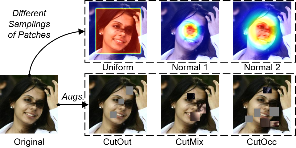
Figure 6: The illustration of patches sampling with different distributions, and the novel pose-irrelevant cut-occlusion (CutOcc) augmentation.

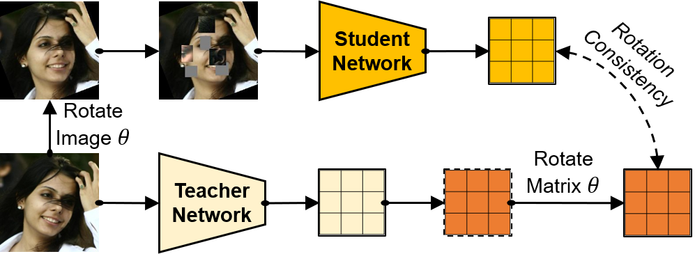
Figure 7: The illustration of proposed pose-altering rotation consistency (RotCons) augmentation. CutMix-related patches are fetched from other samples in the same mini-batch.

Pose-Irrelevant Cut-Occlusion Firstly, we explore pose-irrelevant augmentations such as popular CutOut [13], Mixup [71] and CutMix [67]. CutOut simulates random occlusion. Mixup combines global features in different samples. CutMix balances both occlusion and crossed features. Considering that self- or emerged-occlusion is common in wild heads, we extend the CutOut and CutMix by sampling target patches with head-centered distributions. Heuristically, we provide three proposals of sampling distribution $\mathcal{S}$: Uniform distribution with a small distance from the boundary ($\mathcal{S}_{\mathsf{Uniform}}$), Normal distribution with a smaller variance ($\mathcal{S}_{\mathsf{Normal1}}$) and a larger variance ($\mathcal{S}_{\mathsf{Normal2}}$). Among them, we verified in experiments that the $\mathcal{S}_{\mathsf{Normal2}}$ is superior for its stronger head-centered concentration of noise addition. Then, we propose to conduct CutOut and CutMix in sequence to obtain an advanced combination named Cut-Occlusion (CutOcc). The motivation is to leverage the synergistic effect between two existing components. As shown in Fig. 7, CutOcc is also visually understandable.

Pose-Altering Rotation Consistency Although HPE is sensitive to rotation, we can still perform in-plane rotation augmentation in $\mathcal{SO}$(3) similar to SSL keypoints detection [44, 59, 23]. For a batch of unlabeled heads $\{\mathbf{x}^{u}_{i}\}^{B_{u}}_{i=1}$, we present unsupervised rotation consistency augmentation as shown in Fig. 7. On one hand, we rotate each $\mathbf{x}^{u}_{i}$ with a random angle $\theta$ from $(-30^{\circ},30^{\circ})$, with selectively conducting the subsequent pose-irrelevant operation CutOcc. The strongly augmented $\overline{\mathbf{x}^{u}}$ are then fed into the student model $\mathcal{N}_{stu}$, which outputs parameters in the form of matrix $\overline{p^{i}_{stu}}\in\mathbb{R}^{3\times 3}$. On the other hand, we directly feed weakly augmented $\widetilde{\mathbf{x}^{u}}$ into the teacher model $\mathcal{N}_{tea}$, and obtain the predicted matrix $\widetilde{p^{i}_{tea}}$. Then, we need to rotate $\widetilde{p^{i}_{tea}}$ around the Z-axis with corresponding degree for consistency training. We summarize these steps as follows.

$$\overline{p^{i}_{stu}}=\mathcal{MF}(\mathcal{N}_{stu}(\overline{\mathbf{x}^{u}_{i}})),\quad\overline{\mathbf{x}^{u}_{i}}=T_{\mathsf{CutOcc}}(T_{\mathsf{Rot}_{\theta}}(\mathbf{x}^{u}_{i}))$$ (7)

$$\widetilde{p^{i}_{tea}}=\mathcal{MF}(\mathcal{N}_{tea}(\widetilde{\mathbf{x}^{u}_{i}})),\quad\widetilde{\mathbf{x}^{u}_{i}}=T_{\mathsf{weak}}(\mathbf{x}^{u}_{i})$$

$$\widehat{p^{i}_{tea}}=\mathbf{M_{\theta}}\widetilde{p^{i}_{tea}},\quad\mathbf{M_{\theta}}=\small{\left[\begin{array}[]{ccc}\cos(\theta)&\sin(\theta)&0\\ -\sin(\theta)&\cos(\theta)&0\\ 0&0&1\end{array}\right]}$$

where $T_{\mathsf{CutOcc}}$ and $T_{\mathsf{Rot}_{\theta}}$ means our proposed strong augmentations CutOcc and in-plane rotation, respectively. $\mathbf{M_{\theta}}$ represents the in-plane rotation matrix corresponding to $\theta$. And $\widehat{p^{i}_{tea}}$ is the aligned prediction. We finally enforce consistency between distributions $\widehat{p^{i}_{tea}}$ and $\overline{p^{i}_{stu}}$.

3.6 Training Protocol

Our training has two consecutive phases. Phase1: We train the student model $\mathcal{N}_{stu}$ to learn a rotation regressor on labeled set $\mathcal{D}^{l}$ with a supervised loss:

$$\small\mathcal{L}_{sup}(\mathbf{x}^{l},\mathbf{y}^{l})=-\log(\mathcal{MF}(\mathbf{y}^{l};\mathcal{N}_{stu}(\mathbf{x}^{l}))$$ (8)

where $-\log(\cdot)$ means the negative log likelihood (NLL) of the mode predicted by $\mathcal{N}_{stu}$ in the distribution of ground-truth label $\mathbf{y}^{l}$. We save the best performed student model for cloning an identical teacher model for the next phase.

Phase2: After supervised training, we obtain a pair of teacher and student networks with the same initialization. Now, we begin the semi-supervised phase on both labeled set $\mathcal{D}^{l}$ and unlabeled set $\mathcal{D}^{u}$. The total loss is:

$$\small\mathcal{L}=\mathcal{L}_{sup}(\mathbf{x}^{l},\mathbf{y}^{l})+\lambda\mathcal{L^{\prime}}_{unsup}(\mathbf{x}^{u})$$ (9)

where $\mathcal{L}_{sup}$ and $\mathcal{L^{\prime}}_{unsup}$ are calculated as in Eq. 8 and Eq. 6, respectively. The $\lambda$ is a weight of unsupervised loss, which is set to 1 in all experiments. Besides, we usually allocate different iterations for two phases based on the complexity of labeled $\mathcal{D}^{l}$ and unlabeled $\mathcal{D}^{u}$ datasets.

4 Experiment

4.1 Datasets and Implementation Details

We introduce two kinds of datasets. Labeled: we adopt the popular benchmark 300W-LP [76] which has 122,450 samples with half flipping as the train-set and AFLW2000 [76] as the val-set for comparing with the mainstream front-range HPE methods. We also utilize dataset DAD-3DHeads [34] with three subsets (37,840 images in train-set, 4,312 images in val-set, and 2,746 images in test-set) for implementing the full-range unconstrained HPE. Unlabeled: we utilize COCO [31] with wild human heads as the unlabeled set for boosting both the front-range and full-range HPE. COCO does not have the head box label. We utilize its variation COCO-HumanParts [62] with labeled head boxes, and preprocess it as in BPJDet [72, 74] to generate COCOHead, which has about 74K samples after removing heads smaller than 30 pixels. These left heads cover diverse scenarios and cases. Examples can be found in Fig. 1 and Fig. 2.

Then, we implemented all experiments using PyTorch on 4 RTX 3090 GPUs. Adam optimizer is used. The learning rate in Phase1 is 1e-4, and reduced to 1e-5 in Phase2. The network backbone is either ResNet50 [19] or RepVGG [14]. Then, we designed following three SSL settings:

Setting1: 300W-Self In this setting, we use partially labeled 300W-LP and the left part as the unlabeled set. The labeled ratio is from (2%, 5%, 10%, 20%). In addition to training SemiUHPE with proposed strategies, we also implement the supervised version using only labeled data and the baseline FisherMatch [65]. The Phase1 and Phase2 has 20K and 40K iterations, respectively. The number of threshold updating stages $K$ in Phase2 is 4. Batch size for the labeled set $B_{l}$ and unlabeled set $B_{u}$ is 32 and 128, respectively. The remained percentage $\delta$ of unlabeled data is 0.95. The test-set is AFLW2000. For a fair comparison, we keep samples with Euler angles within $\pm 90^{\circ}$ following the previous front-range HPE methods. The evaluation metric is Mean Absolute Error (MAE) of Euler angles. We thus convert predictions into Euler angles for comparing.

Setting2: 300W-COCO Still for the front-range HPE, we combine all labeled 300W-LP with additional unlabeled faces in WiderFace for further performance boosting. We set Phase1 and Phase2 with 180K and 60K iterations, respectively. Parameters $K$, $B_{l}$, $B_{u}$ and $\delta$ are set to 6, 16, 128 and 0.75, respectively. The test-set is AFLW2000. The others are the same as Setting1.

Setting3: DAD-COCO This is for the full-range HPE task. We use the train-set of DAD-3DHeads as the labeled set, and COCOHead as the unlabeled set. We set Phase1 and Phase2 with 100K and 100K iterations, respectively. And parameters $K$, $B_{l}$, $B_{u}$ and $\delta$ are set to 5, 16, 128 and 0.75, respectively. We report testing results on both val-set and test-set of DAD-3DHeads. Following [34], measures of the ground-truth matrix $\mathbf{R}_{1}$ and predicted $\mathbf{R}_{2}$ are (1) Frobenius norm of the matrix $\mathbf{I}\!-\!\mathbf{R}_{1}\mathbf{R}_{2}^{T}$, and (2) the angle in axis-angle representation of $\mathbf{R}_{1}\mathbf{R}_{2}^{T}$ (a.k.a the geodesic distance between two rotation matrices).

4.2 Quantitative Comparison

Below, we report results with above-defined settings. The supervised and baseline are implemented with using the proposed aspect-ratio invariant cropping.

Setting1 As shown in Table 1, our SemiUHPE can surpass both the supervised methods and baseline FisherMatch [65] with either backbone. Meanwhile, the smaller the ratio of labeled samples used (from 20% to 2%), the more significant the reduction in MAE errors. Moreover, with using 20% labeled 300W-LP, the performance of semi-supervised baseline and SemiUHPE can exceed the supervised method using all labeled 300W-LP. We attribute this to the stronger robustness brought about by partially integrated unsupervised training. It also indicates that pure supervised learning may cause model overfitting on the train-set, while SSL can improve the generalization to a certain extent.

Setting2 As shown in Table 2, with supporting of SSL, our method based on the ordinary ResNet50 can achieve a low MAE result 3.37, which is comparable to other supervised SOTA front-range HPE methods such as DAD-3DNet [34] with MAE 3.66, SynergyNet [56] with MAE 3.35 and DSFNet-f [30] with MAE 3.25. Please note that all of them are 3DMM-based which require dense face landmark labels and complex 3D face reconstruction. While, our SemiUHPE only requires reasonable excavation of unlabeled wild heads, which is more practical and scalable in real applications. When using a stronger backbone RepVGG as in 6DRepNet [20], our method can obtain a lower result with MAE 3.35, which further explains its generality and advantage.

Setting3 As shown in Table 3, results of Img2Pose [4] and DAD-3DNet [34] are from the paper [34], except for results of DAD-3DNet on the val-set which are evaluated by us using its official model. The supervised method is trained on DAD-3DHeads train-set by us. Generally, our SemiUHPE significantly surpasses the compared method DAD-3DNet and retrained baselines without using any 3D information of face or head, which again proves its superiority and versatility. Moreover, we give detailed comparison under different challenging conditions in Table 4. Our method is still clearly ahead. Without bells and whistles, we achieved SOTA full-range HPE results on DAD-3DHeads.

Table 1: Euler angles errors on AFLW2000. Models are trained on 300W-LP with different ratios of label. The best result is in red color.

Method	Backbone	2%	5%	10%	20%	All
Supervised	ResNet50	4.347	3.987	3.831	3.619	3.578
Supervised	RepVGG	4.252	3.817	3.724	3.579	3.498
Baseline [65]	ResNet50	4.190	3.798	3.609	3.492	—
Baseline [65]	RepVGG	4.023	3.730	3.489	3.445	—
SemiUHPE	ResNet50	3.956	3.629	3.487	3.463	—
SemiUHPE	RepVGG	3.953	3.607	3.510	3.424	—

Table 2: Euler angles errors on AFLW2000. Models are all trained on 300W-LP. Extra means using other annotations such as face Landmarks (LMs) or 3D Morphable Model (3DMM). The best and second-best result is in red and blue color, respectively.

Method	Reference	Extra	Pitch	Yaw	Roll	MAE
3DDFA [76]	CVPR’16	3DMM	5.98	4.33	4.30	4.87
HopeNet [46]	CVPRW’18	No	6.56	6.47	5.44	6.16
QuatNet [21]	TMM’18	No	5.62	3.97	3.92	4.50
FSA-Net [64]	CVPR’19	No	6.08	4.50	4.64	5.07
WHENet-V [75]	BMVC’20	No	5.75	4.44	4.31	4.83
FDN [70]	AAAI’20	No	5.61	3.78	3.88	4.42
3DDFA-V2 [18]	ECCV’20	3DMM	5.26	4.06	3.48	4.27
MNN [51]	TPAMI’20	LMs	4.69	3.34	3.48	3.83
Rankpose [10]	BMVC’20	No	4.75	2.99	3.25	3.66
TriNet [8]	WACV’21	No	5.77	4.20	4.04	4.67
MFDNet [32]	TMM’21	No	5.16	4.30	3.69	4.38
Img2Pose [4]	CVPR’21	LMs	5.03	3.43	3.28	3.91
SADRNet [45]	TIP’21	3DMM	5.00	2.93	3.54	3.82
SynergyNet [56]	3DV’21	3DMM	4.09	3.42	2.55	3.35
6DRepNet [20]	ICIP’22	No	4.91	3.63	3.37	3.97
DAD-3DNet [34]	CVPR’22	3DMM	4.76	3.08	3.15	3.66
TokenHPE [69]	CVPR’23	No	5.54	4.36	4.08	4.66
DSFNet-f [30]	CVPR’23	3DMM	4.28	2.65	2.82	3.25
Baseline [65] (ResNet50)	CVPR’22	No	4.61	2.99	3.00	3.53
Baseline [65] (RepVGG)	CVPR’22	No	4.46	2.84	2.77	3.36
Ours (ResNet50)	—	No	4.52	2.89	2.71	3.37
Ours (RepVGG)	—	No	4.43	2.86	2.75	3.35

Table 3: HPE results on the val-set and test-set of challenging DAD-3DHeads dataset.

Method	$\|\mathbf{I}\!-\!\mathbf{R}_{1}\mathbf{R}_{2}^{T}\|_{F}\!\downarrow$		Angle error (degree)$\downarrow$
	val-set	test-set	val-set	test-set
Img2Pose [4]	—	0.226	—	9.122
DAD-3DNet [34]	0.130	0.138	5.456	5.360
Supervised (ResNet50)	0.133	0.138	5.543	5.234
Supervised (RepVGG)	0.128	0.134	5.321	5.020
Baseline [65] (ResNet50)	0.139	0.145	5.859	5.312
Baseline [65] (RepVGG)	0.129	0.137	5.369	5.182
Ours (ResNet50)	0.116	0.127	4.800	4.810
Ours (RepVGG)	0.116	0.126	4.778	4.760

Table 4: Detailed HPE errors ($\|\mathbf{I}\!-\!\mathbf{R}_{1}\mathbf{R}_{2}^{T}\|_{F}\!\downarrow$ / Angle error (degree)$\downarrow$) on DAD-3DHeads test-set with three subsets: challenging atypical poses (Pose), compound expressions (Expr.) and heavy occlusions (Occl.).

Method	Overall	Pose	Expr.	Occl.
3DDFA-V2 [18]	0.527 /   —–	0.790 /   —–	0.455 /   —–	0.542 /   —–
RingNet [47]	0.438 /   —–	1.076 /   —–	0.294 /   —–	0.551 /   —–
DAD-3DNet [34]	0.138 / 5.360	0.343 /   —–	0.112 /   —–	0.203 /   —–
Supervised (ResNet50)	0.138 / 5.234	0.327 / 10.782	0.111 / 4.351	0.181 / 7.134
Supervised (RepVGG)	0.134 / 5.020	0.325 /   9.961	0.108 / 4.233	0.179 / 6.880
Baseline [65] (ResNet50)	0.145 / 5.312	0.400 / 11.109	0.111 / 4.356	0.194 / 7.583
Baseline [65] (RepVGG)	0.137 / 5.182	0.349 / 10.932	0.110 / 4.305	0.176 / 7.175
Ours (ResNet50)	0.127 / 4.810	0.322 /   9.581	0.103 / 4.106	0.159 / 6.463
Ours (RepVGG)	0.126 / 4.760	0.307 /   9.110	0.105 / 4.180	0.149 / 6.041

4.3 Performance Improvement Analysis

To systematically understand the source of improvement after boosting the baseline FisherMatch with our proposed various strategies, we further calculate and plot the head pose error gains on datasets AFLW2000 for front-range HPE and DAD-3DHeads for full-range HPE. As shown in Fig. 8, we split all the testing images into different groups according to their GT yaw angles and calculate the improved error degree within each group. We can find that the improvement by our SemiUHPE gets more obvious as the head pose gets more challenging.

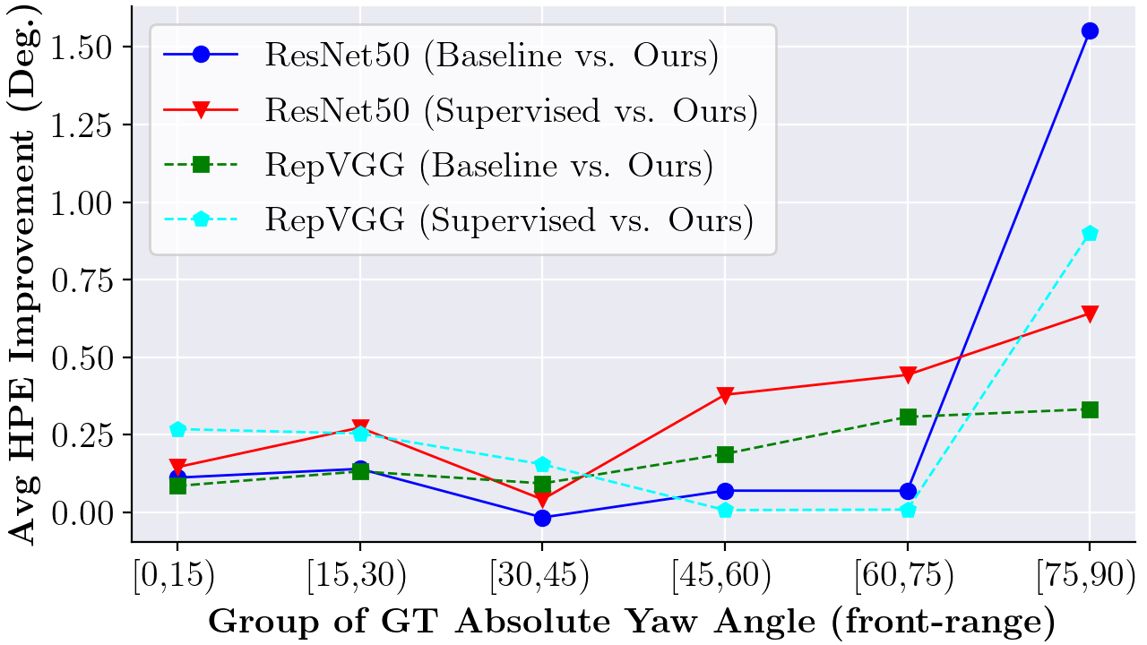
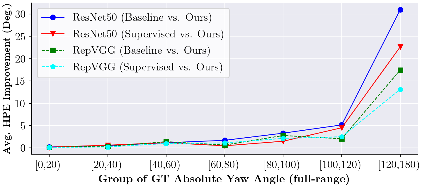
Figure 8: The HPE improvement on AFLW2000 (left) and DAD-3DHeads val-set (right).

4.4 Ablation Studies

We give detailed studies for explaining the effect of our proposed strategies.

Aspect-Ratio Invariant Cropping We took FSA-Net [64] and 6DRepNet [20] using the naive cropping-resizing for comparing. Then, we replaced them with our aspect-ratio invariant cropping, and retrained new versions FSA-Net${\dagger}$ and 6DRepNet${\dagger}$. We also listed results of the trivial supervised method. As shown in Table 5, both the original FSA-Net and 6DRepNet are significantly improved. When using RepVGG and new cropping, 6DRepNet${\dagger}$ can even compete with the supervised method using an advanced matrix Fisher representation. These prove the superiority of using this simple yet efficient size-invariant preprocessing.

Dynamic Entropy-based Filtering We designed three groups of experiments for explaining the effectiveness of dynamic filtering strategy. In Fig. 9(a), we searched for the optimal pre-fixed threshold $\tau$ used by FisherMatch. Nonetheless, our dynamic threshold $\tau_{k}$ with $\delta\!=\!0.95$ got the best result. We also searched for the optimal $\delta$ for different unlabeled datasets. In Fig. 9(b), we got the optimal $\delta\!=\!0.95$, which is a large ratio due to that both labeled and unlabeled data are in 300W-LP. In Fig. 9(d), we got a lower optimal $\delta\!=\!0.75$, which is caused by more difficult and noisy heads in the unlabeled COCOHead. Usually, an ideal $\delta$ should equal to $1\!-\!\|\mathcal{D}^{u}_{ood}\|/\|\mathcal{D}^{u}\|$. But we cannot obtain the accurate ratio of $\mathcal{D}^{u}_{ood}$ in $\mathcal{D}^{u}$. We thus estimated a suitable $\delta$ by ablation studies. For example, the optimal $\delta$ of COCOHead is 0.75 in Setting2 and Setting3, which means $\delta$ may be dataset-related yet not sensitive to task settings.

Head-Oriented Strong Augmentations We conducted two groups of experiments for showing the effectiveness of new strong augmentations. In Fig. 9(c), we can see that CutMix is always better than CutOut. The best sampling distribution is $\mathcal{S}_{\mathsf{Normal2}}$ for its reasonable concentration of occlusion generation. Keep using $\mathcal{S}_{\mathsf{Normal2}}$, in Fig. 9(e), we observed the same effect of CutOut and CutMix. When combining them together, the new $T_{\mathsf{CutOcc}}$ can further reduce HPE errors. Independently, the proposed rotation consistency augmentation $T_{\mathsf{Rot}_{\theta}}$ can also improve performance. Finally, when applying both $T_{\mathsf{CutOcc}}$ and $T_{\mathsf{Rot}_{\theta}}$, we achieved the best result with a remarkable promotion.

Influence of Unsupervised Loss Weight As shown in Fig. 9(f), we selected the unsupervised loss weight $\lambda$ from (0.1, 0.2, 0.5, 1.0, 1.5, 2.0). Our method performed best when $\lambda\!=\!1.0$, which indicates that it does not require careful adjustments of the unsupervised part weight.

Table 5: MAE results of Euler angles on the AFLW2000. Models are trained on 300W-LP with different input copping ways and rotation representations.

Method	Backbone	Cropping	Rot-Rep	Pitch	Yaw	Roll	MAE
FSA-Net [64]	ResNet50	Naive	Euler angles	6.08	4.50	4.64	5.07
FSA-Net${\dagger}$ [64]	ResNet50	Ours	Euler angles	5.42	4.01	3.75	4.39
6DRepNet [20]	RepVGG	Naive	trivial matrix	4.91	3.63	3.37	3.97
6DRepNet${\dagger}$ [20]	RepVGG	Ours	trivial matrix	4.58	3.04	2.86	3.49
Supervised	ResNet50	Ours	matrix Fisher	4.58	3.20	2.95	3.58
Supervised	RepVGG	Ours	matrix Fisher	4.50	3.18	2.81	3.50

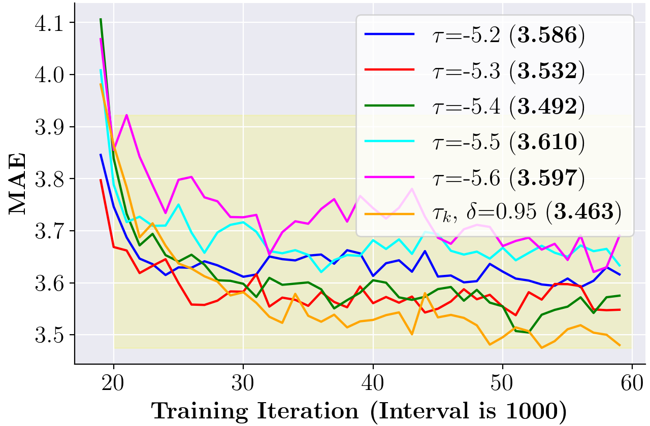
(a)  

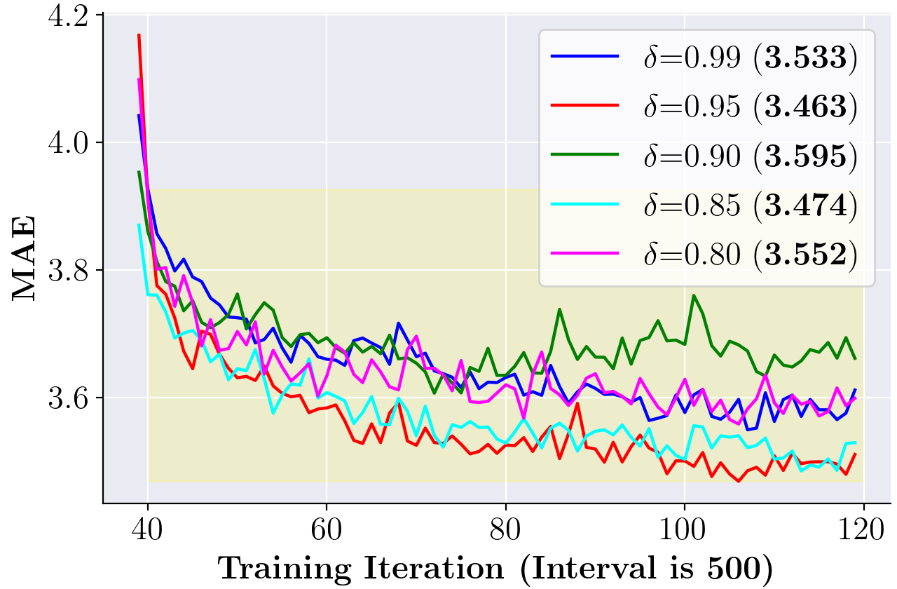
(b)  

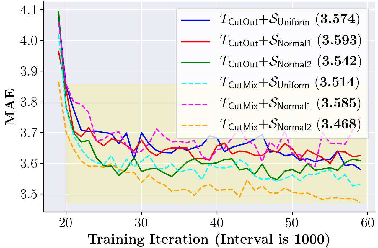
(c)  

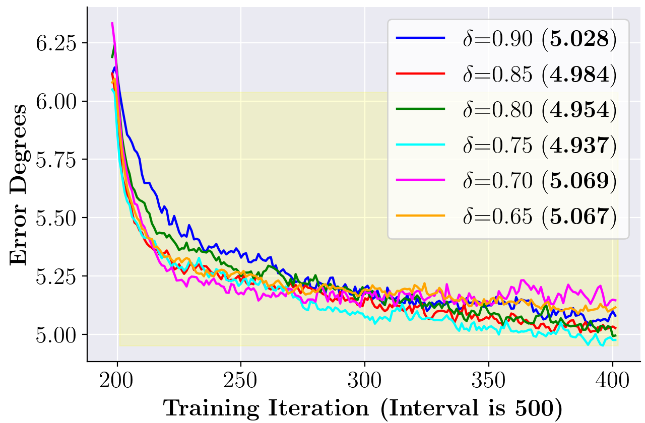
(d)  

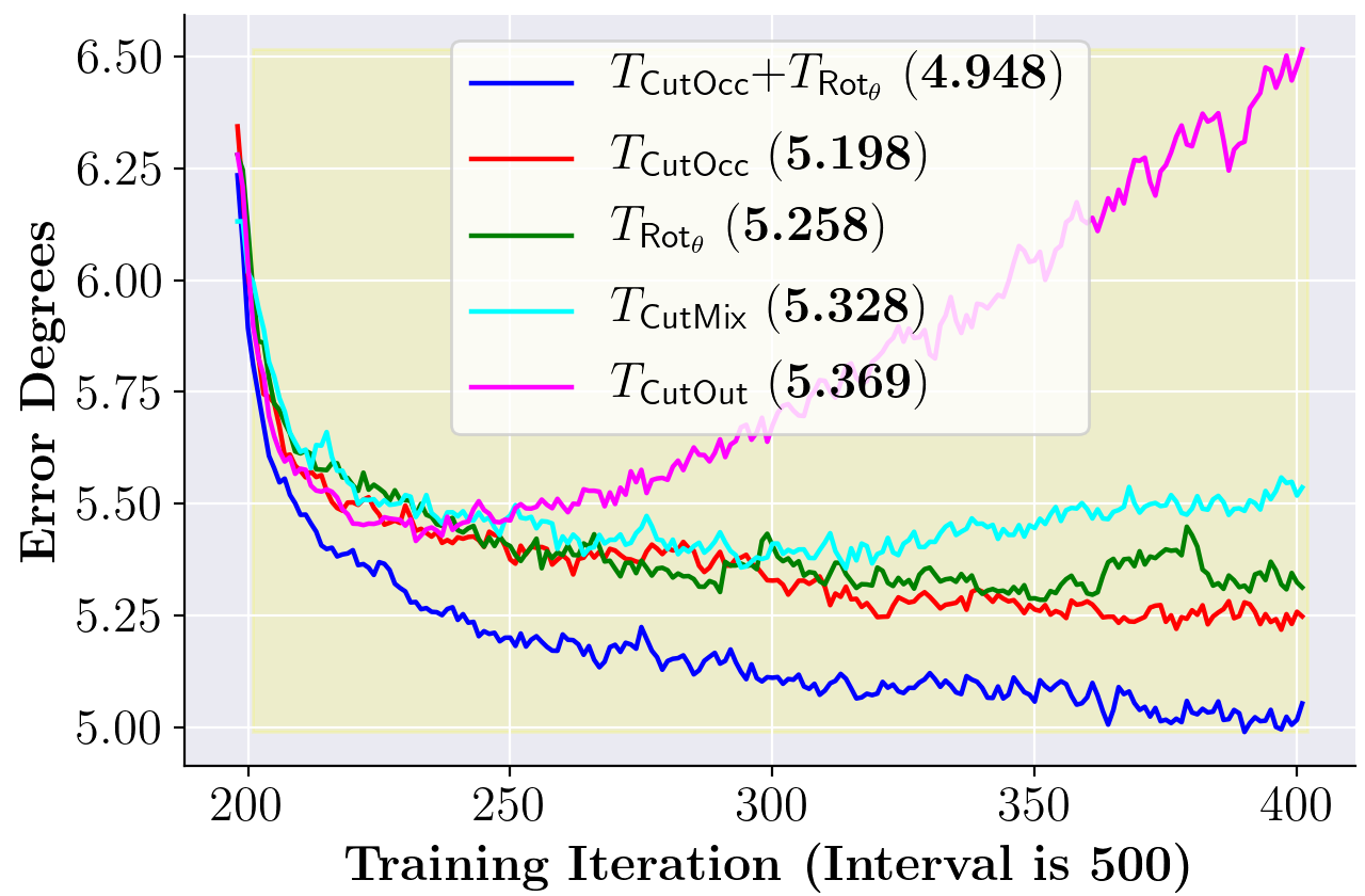
(e)  

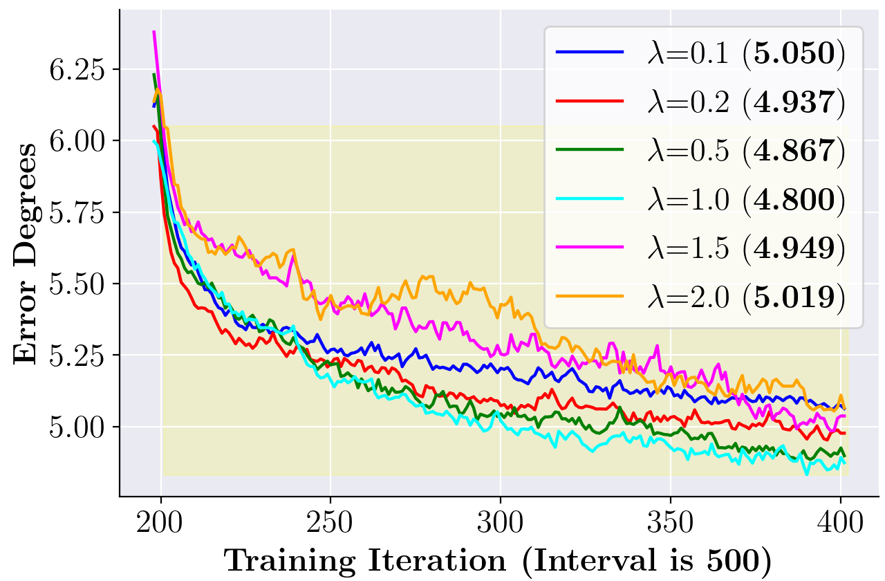
(f)  

Figure 9: The backbone of each model is ResNet50. The bold number within parentheses is the best result. We mainly show results in Phase2. Top: Setting1 with 20% labels. (a) The comparison of using a dynamic threshold $\tau_{k}$ with $\delta\!=\!0.95$ or pre-fixed threshold $\tau$. (b) The influence of $\delta$. (c) The effect of different sampling ways. Bottom: Setting3. (d) The influence of $\delta$ with $\lambda\!=\!0.2$. (e) The effect of different augmentations with $\lambda\!=\!0.2$ and $\delta\!=\!0.75$. (f) The influence of $\lambda$ with $\delta\!=\!0.75$.

4.5 Qualitative Comparison

To further explain the superiority of our SemiUHPE, we present the qualitative comparison with SOTA counterparts including SynergyNet [56], DAD-3DNet [34] and DSFNet-f [30]. As shown in Fig. 10, our method can obtain impressive HPE results on wild challenging heads. Moreover, we present comparison on never-before-experienced yet challenging samples from the test-set of DAD-3DHeads. As shown in Fig. 11, although these images have high-definition, DAD-3DNet may make significant mistakes, leading to disordered results of head reconstruction. While, our method usually gives a satisfactory estimation. More convincing qualitative results are in our supplementary paper.

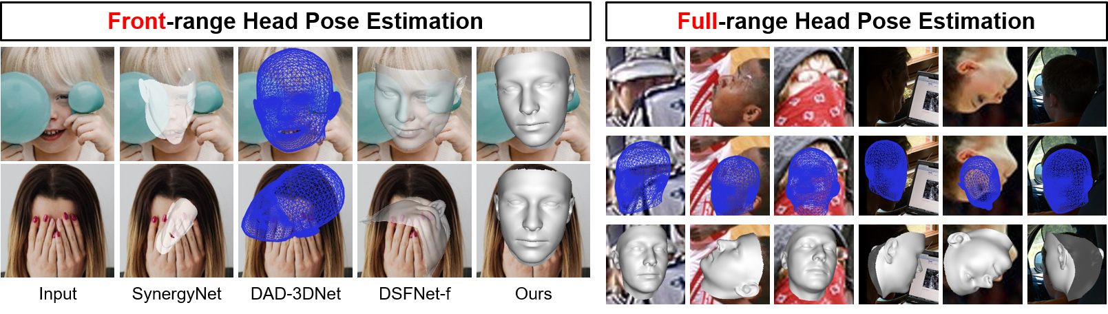
Figure 10: Visualizations of front-range or full-range head pose estimation (HPE). Our method is more robust to severe occlusion, atypical pose and invisible face.

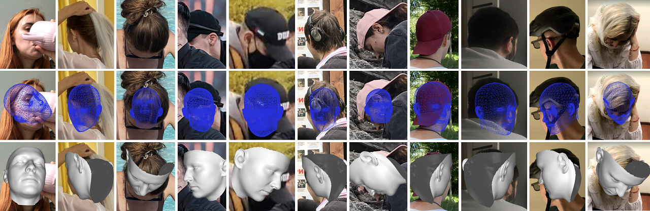
Figure 11: Qualitative results of our method (1st line) and DAD-3DNet [34] (2nd line) on heads from DAD-3DHeads test-set, which never appeared during SSL training.

5 Conclusion

In this paper, we aim to address the unconstrained head pose estimation task on less-touched wild head images. Due to the lack of corresponding labels, we turn to semi-supervised learning techniques. Based on empirically effective frameworks, we propose the dynamic entropy-based filtering for gradually updating thresholds and head-oriented strong augmentations for better enforcing consistency training. By combining the aspect-ratio invariant cropping, our proposed method SemiUHPE can achieve optimal HPE performance quantitatively and qualitatively on omnidirectional wild heads. We expect that our work will greatly inspire and promote related downstream applications.

References

- [1] Abate, A.F., Bisogni, C., Castiglione, A., Nappi, M.: Head pose estimation: An extensive survey on recent techniques and applications. PR 127, 108591 (2022)
- [2] Ahuja, K., Kim, D., Xhakaj, F., Varga, V., Xie, A., Zhang, S., Townsend, J.E., Harrison, C., Ogan, A., Agarwal, Y.: Edusense: Practical classroom sensing at scale. UbiComp 3(3), 1–26 (2019)
- [3] Ahuja, K., Shah, D., Pareddy, S., Xhakaj, F., Ogan, A., Agarwal, Y., Harrison, C.: Classroom digital twins with instrumentation-free gaze tracking. In: CHI. pp. 1–9 (2021)
- [4] Albiero, V., Chen, X., Yin, X., Pang, G., Hassner, T.: img2pose: Face alignment and detection via 6dof, face pose estimation. In: CVPR. pp. 7617–7627 (2021)
- [5] Berthelot, D., Carlini, N., Goodfellow, I., Papernot, N., Oliver, A., Raffel, C.A.: Mixmatch: A holistic approach to semi-supervised learning. NeurIPS 32 (2019)
- [6] Bulat, A., Tzimiropoulos, G.: How far are we from solving the 2d & 3d face alignment problem?(and a dataset of 230,000 3d facial landmarks). In: ICCV. pp. 1021–1030 (2017)
- [7] Cantarini, G., Tomenotti, F.F., Noceti, N., Odone, F.: Hhp-net: A light heteroscedastic neural network for head pose estimation with uncertainty. In: WACV. pp. 3521–3530 (2022)
- [8] Cao, Z., Chu, Z., Liu, D., Chen, Y.: A vector-based representation to enhance head pose estimation. In: WACV. pp. 1188–1197 (2021)
- [9] Chen, Y., Tan, X., Zhao, B., Chen, Z., Song, R., Liang, J., Lu, X.: Boosting semi-supervised learning by exploiting all unlabeled data. In: CVPR. pp. 7548–7557 (2023)
- [10] Dai, D., Wong, W., Chen, Z.: Rankpose: Learning generalised feature with rank supervision for head pose estimation. In: BMVC (2020)
- [11] Deng, J., Guo, J., Ververas, E., Kotsia, I., Zafeiriou, S.: Retinaface: Single-shot multi-level face localisation in the wild. In: CVPR. pp. 5203–5212 (2020)
- [12] Deng, J., Guo, J., Xue, N., Zafeiriou, S.: Arcface: Additive angular margin loss for deep face recognition. In: CVPR. pp. 4690–4699 (2019)
- [13] DeVries, T., Taylor, G.W.: Improved regularization of convolutional neural networks with cutout. arXiv preprint arXiv:1708.04552 (2017)
- [14] Ding, X., Zhang, X., Ma, N., Han, J., Ding, G., Sun, J.: Repvgg: Making vgg-style convnets great again. In: CVPR. pp. 13733–13742 (2021)
- [15] Fanelli, G., Dantone, M., Gall, J., Fossati, A., Van Gool, L.: Random forests for real time 3d face analysis. IJCV 101, 437–458 (2013)
- [16] Geng, X., Qian, X., Huo, Z., Zhang, Y.: Head pose estimation based on multivariate label distribution. TPAMI 44(4), 1974–1991 (2020)
- [17] Gu, J., Yang, X., De Mello, S., Kautz, J.: Dynamic facial analysis: From bayesian filtering to recurrent neural network. In: CVPR. pp. 1548–1557 (2017)
- [18] Guo, J., Zhu, X., Yang, Y., Yang, F., Lei, Z., Li, S.Z.: Towards fast, accurate and stable 3d dense face alignment. In: ECCV. pp. 152–168. Springer (2020)
- [19] He, K., Zhang, X., Ren, S., Sun, J.: Deep residual learning for image recognition. In: CVPR. pp. 770–778 (2016)
- [20] Hempel, T., Abdelrahman, A.A., Al-Hamadi, A.: 6d rotation representation for unconstrained head pose estimation. In: ICIP. pp. 2496–2500. IEEE (2022)
- [21] Hsu, H.W., Wu, T.Y., Wan, S., Wong, W.H., Lee, C.Y.: Quatnet: Quaternion-based head pose estimation with multiregression loss. TMM 21(4), 1035–1046 (2018)
- [22] Hu, Z., Yang, Z., Hu, X., Nevatia, R.: Simple: Similar pseudo label exploitation for semi-supervised classification. In: CVPR. pp. 15099–15108 (2021)
- [23] Huang, L., Li, Y., Tian, H., Yang, Y., Li, X., Deng, W., Ye, J.: Semi-supervised 2d human pose estimation driven by position inconsistency pseudo label correction module. In: CVPR. pp. 693–703 (2023)
- [24] Kao, Y., Pan, B., Xu, M., Lyu, J., Zhu, X., Chang, Y., Li, X., Lei, Z.: Towards 3d face reconstruction in perspective projection: Estimating 6dof face pose from monocular image. TIP (2023)
- [25] Kazemi, V., Sullivan, J.: One millisecond face alignment with an ensemble of regression trees. In: CVPR. pp. 1867–1874 (2014)
- [26] Kim, J., Jang, J., Seo, S., Jeong, J., Na, J., Kwak, N.: Mum: Mix image tiles and unmix feature tiles for semi-supervised object detection. In: CVPR. pp. 14512–14521 (2022)
- [27] Kuhnke, F., Ostermann, J.: Deep head pose estimation using synthetic images and partial adversarial domain adaption for continuous label spaces. In: CVPR. pp. 10164–10173 (2019)
- [28] Laine, S., Aila, T.: Temporal ensembling for semi-supervised learning. In: ICLR (2016)
- [29] Levinson, J., Esteves, C., Chen, K., Snavely, N., Kanazawa, A., Rostamizadeh, A., Makadia, A.: An analysis of svd for deep rotation estimation. NeurIPS 33, 22554–22565 (2020)
- [30] Li, H., Wang, B., Cheng, Y., Kankanhalli, M., Tan, R.T.: Dsfnet: Dual space fusion network for occlusion-robust 3d dense face alignment. In: CVPR. pp. 4531–4540 (2023)
- [31] Lin, T.Y., Maire, M., Belongie, S., Hays, J., Perona, P., Ramanan, D., Dollár, P., Zitnick, C.L.: Microsoft coco: Common objects in context. In: ECCV. pp. 740–755. Springer (2014)
- [32] Liu, H., Fang, S., Zhang, Z., Li, D., Lin, K., Wang, J.: Mfdnet: Collaborative poses perception and matrix fisher distribution for head pose estimation. TMM 24, 2449–2460 (2021)
- [33] Liu, W., Wen, Y., Yu, Z., Li, M., Raj, B., Song, L.: Sphereface: Deep hypersphere embedding for face recognition. In: CVPR. pp. 212–220 (2017)
- [34] Martyniuk, T., Kupyn, O., Kurlyak, Y., Krashenyi, I., Matas, J., Sharmanska, V.: Dad-3dheads: A large-scale dense, accurate and diverse dataset for 3d head alignment from a single image. In: CVPR. pp. 20942–20952 (2022)
- [35] Mohlin, D., Sullivan, J., Bianchi, G.: Probabilistic orientation estimation with matrix fisher distributions. NeurIPS 33, 4884–4893 (2020)
- [36] Murphy-Chutorian, E., Trivedi, M.M.: Head pose estimation in computer vision: A survey. TPAMI 31(4), 607–626 (2008)
- [37] Murphy-Chutorian, E., Trivedi, M.M.: Head pose estimation and augmented reality tracking: An integrated system and evaluation for monitoring driver awareness. TITS 11(2), 300–311 (2010)
- [38] Nassar, I., Hayat, M., Abbasnejad, E., Rezatofighi, H., Haffari, G.: Protocon: Pseudo-label refinement via online clustering and prototypical consistency for efficient semi-supervised learning. In: CVPR. pp. 11641–11650 (2023)
- [39] Nassar, I., Herath, S., Abbasnejad, E., Buntine, W., Haffari, G.: All labels are not created equal: Enhancing semi-supervision via label grouping and co-training. In: CVPR. pp. 7241–7250 (2021)
- [40] Nonaka, S., Nobuhara, S., Nishino, K.: Dynamic 3d gaze from afar: Deep gaze estimation from temporal eye-head-body coordination. In: CVPR. pp. 2192–2201 (2022)
- [41] Oliver, A., Odena, A., Raffel, C.A., Cubuk, E.D., Goodfellow, I.: Realistic evaluation of deep semi-supervised learning algorithms. NeurIPS 31 (2018)
- [42] Radosavovic, I., Dollár, P., Girshick, R., Gkioxari, G., He, K.: Data distillation: Towards omni-supervised learning. In: CVPR. pp. 4119–4128 (2018)
- [43] Ranjan, R., Patel, V.M., Chellappa, R.: Hyperface: A deep multi-task learning framework for face detection, landmark localization, pose estimation, and gender recognition. TPAMI 41(1), 121–135 (2017)
- [44] Rhodin, H., Salzmann, M., Fua, P.: Unsupervised geometry-aware representation for 3d human pose estimation. In: ECCV. pp. 750–767 (2018)
- [45] Ruan, Z., Zou, C., Wu, L., Wu, G., Wang, L.: Sadrnet: Self-aligned dual face regression networks for robust 3d dense face alignment and reconstruction. TIP 30, 5793–5806 (2021)
- [46] Ruiz, N., Chong, E., Rehg, J.M.: Fine-grained head pose estimation without keypoints. In: CVPRW. pp. 2074–2083 (2018)
- [47] Sanyal, S., Bolkart, T., Feng, H., Black, M.J.: Learning to regress 3d face shape and expression from an image without 3d supervision. In: CVPR. pp. 7763–7772 (2019)
- [48] Shao, S., Zhao, Z., Li, B., Xiao, T., Yu, G., Zhang, X., Sun, J.: Crowdhuman: A benchmark for detecting human in a crowd. arXiv preprint arXiv:1805.00123 (2018)
- [49] Sohn, K., Berthelot, D., Carlini, N., Zhang, Z., Zhang, H., Raffel, C.A., Cubuk, E.D., Kurakin, A., Li, C.L.: Fixmatch: Simplifying semi-supervised learning with consistency and confidence. NeurIPS 33, 596–608 (2020)
- [50] Tarvainen, A., Valpola, H.: Mean teachers are better role models: Weight-averaged consistency targets improve semi-supervised deep learning results. NeurIPS 30 (2017)
- [51] Valle, R., Buenaposada, J.M., Baumela, L.: Multi-task head pose estimation in-the-wild. TPAMI 43(8), 2874–2881 (2020)
- [52] Wang, A., Mei, S., Yuille, A.L., Kortylewski, A.: Neural view synthesis and matching for semi-supervised few-shot learning of 3d pose. NeurIPS 34, 7207–7219 (2021)
- [53] Wang, G., Manhardt, F., Liu, X., Ji, X., Tombari, F.: Occlusion-aware self-supervised monocular 6d object pose estimation. TPAMI (2021)
- [54] Wang, G., Manhardt, F., Shao, J., Ji, X., Navab, N., Tombari, F.: Self6d: Self-supervised monocular 6d object pose estimation. In: ECCV. pp. 108–125. Springer (2020)
- [55] Wang, Y., Zhou, W., Zhou, J.: 2dheadpose: A simple and effective annotation method for the head pose in rgb images and its dataset. NN 160, 50–62 (2023)
- [56] Wu, C.Y., Xu, Q., Neumann, U.: Synergy between 3dmm and 3d landmarks for accurate 3d facial geometry. In: 3DV. pp. 453–463. IEEE (2021)
- [57] Wu, J., Yang, H., Gan, T., Ding, N., Jiang, F., Nie, L.: Chmatch: Contrastive hierarchical matching and robust adaptive threshold boosted semi-supervised learning. In: CVPR. pp. 15762–15772 (2023)
- [58] Xie, Q., Dai, Z., Hovy, E., Luong, T., Le, Q.: Unsupervised data augmentation for consistency training. NeurIPS 33, 6256–6268 (2020)
- [59] Xie, R., Wang, C., Zeng, W., Wang, Y.: An empirical study of the collapsing problem in semi-supervised 2d human pose estimation. In: ICCV. pp. 11240–11249 (2021)
- [60] Yang, F., Wu, K., Zhang, S., Jiang, G., Liu, Y., Zheng, F., Zhang, W., Wang, C., Zeng, L.: Class-aware contrastive semi-supervised learning. In: CVPR. pp. 14421–14430 (2022)
- [61] Yang, L., Qi, L., Feng, L., Zhang, W., Shi, Y.: Revisiting weak-to-strong consistency in semi-supervised semantic segmentation. In: CVPR. pp. 7236–7246 (2023)
- [62] Yang, L., Song, Q., Wang, Z., Hu, M., Liu, C.: Hier r-cnn: Instance-level human parts detection and a new benchmark. TIP pp. 39–54 (2020)
- [63] Yang, S., Luo, P., Loy, C.C., Tang, X.: Wider face: A face detection benchmark. In: CVPR. pp. 5525–5533 (2016)
- [64] Yang, T.Y., Chen, Y.T., Lin, Y.Y., Chuang, Y.Y.: Fsa-net: Learning fine-grained structure aggregation for head pose estimation from a single image. In: CVPR. pp. 1087–1096 (2019)
- [65] Yin, Y., Cai, Y., Wang, H., Chen, B.: Fishermatch: Semi-supervised rotation regression via entropy-based filtering. In: CVPR. pp. 11164–11173 (2022)
- [66] Yu, Y., Mora, K.A.F., Odobez, J.M.: Headfusion: 360∘ head pose tracking combining 3d morphable model and 3d reconstruction. TPAMI 40(11), 2653–2667 (2018)
- [67] Yun, S., Han, D., Oh, S.J., Chun, S., Choe, J., Yoo, Y.: Cutmix: Regularization strategy to train strong classifiers with localizable features. In: ICCV. pp. 6023–6032 (2019)
- [68] Zhang, B., Wang, Y., Hou, W., Wu, H., Wang, J., Okumura, M., Shinozaki, T.: Flexmatch: Boosting semi-supervised learning with curriculum pseudo labeling. NeurIPS 34, 18408–18419 (2021)
- [69] Zhang, C., Liu, H., Deng, Y., Xie, B., Li, Y.: Tokenhpe: Learning orientation tokens for efficient head pose estimation via transformers. In: CVPR. pp. 8897–8906 (2023)
- [70] Zhang, H., Wang, M., Liu, Y., Yuan, Y.: Fdn: Feature decoupling network for head pose estimation. In: AAAI. vol. 34, pp. 12789–12796 (2020)
- [71] Zhang, H., Cisse, M., Dauphin, Y.N., Lopez-Paz, D.: mixup: Beyond empirical risk minimization. In: ICLR (2018)
- [72] Zhou, H., Jiang, F., Lu, H.: Body-part joint detection and association via extended object representation. In: ICME. pp. 168–173. IEEE (2023)
- [73] Zhou, H., Jiang, F., Lu, H.: Directmhp: Direct 2d multi-person head pose estimation with full-range angles. arXiv preprint arXiv:2302.01110 (2023)
- [74] Zhou, H., Jiang, F., Si, J., Ding, Y., Lu, H.: Bpjdet: Extended object representation for generic body-part joint detection. TPAMI (2024)
- [75] Zhou, Y., Gregson, J.: Whenet: Real-time fine-grained estimation for wide range head pose. In: BMVC (2020)
- [76] Zhu, X., Lei, Z., Liu, X., Shi, H., Li, S.Z.: Face alignment across large poses: A 3d solution. In: CVPR. pp. 146–155 (2016)