Grid-Mapping Pseudo-Count Constraint for Offline Reinforcement Learning
Abstract
Offline reinforcement learning learns from a static dataset without interacting with the environment, which ensures security and thus owns a good prospect of application. However, directly applying naive reinforcement learning methods usually fails in an offline environment due to function approximation errors caused by out-of-distribution(OOD) actions. To solve this problem, existing algorithms mainly penalize the Q-value of OOD actions, the quality of whose constraints also matter. Imprecise constraints may lead to suboptimal solutions, while precise constraints require significant computational costs. In this paper, we propose a novel count-based method for continuous domains, called Grid-Mapping Pseudo-Count method(GPC), to penalize the Q-value appropriately and reduce the computational cost. The proposed method maps the state and action space to discrete space and constrains their Q-values through the pseudo-count. It is theoretically proved that only a few conditions are needed to obtain accurate uncertainty constraints in the proposed method. Moreover, we develop a Grid-Mapping Pseudo-Count Soft Actor-Critic(GPC-SAC) algorithm using GPC under the Soft Actor-Critic(SAC) framework to demonstrate the effectiveness of GPC. The experimental results on D4RL benchmark datasets show that GPC-SAC has better performance and less computational cost compared to other algorithms.
1 Introduction
In 2023, the release of chatgpt4 and swift openai2023gpt4 ; kaufmann2023champion , once again pushed the achievement of deep reinforcement learning (DRL) to a new peak. In addition to chatbot and automatic operation, DRL has also made remarkable achievements in many other fields in recent years, such as games vinyals2019grandmaster and medical yu2021reinforcement . It is worth noting that the vast majority of them do not require interaction with the physical environment. Why the current achievements of RL in physical environments are still less? That is because DRL is learning what to do—how to map situations to actions—to maximize a numerical reward signal sutton2018reinforcement . In other words, the application of RL in a physical environment requires the interaction between agent and environment, which may cause great damage to the environment or the agent levine2020offline . To this end, offline reinforcement learning (offline RL) has rapidly become a hot research topic considering safety issues. Offline RL, also known as batch RL, only learns policy through static datasets without interacting with the environment, thus guaranteeing safety. Therefore, offline RL is more likely to be applied in physical environments than naive RL fujimoto2019off ; agarwal2020optimistic .
However, there exists a problem called distributional shift when directly applying offline RL in practice. It is mainly attributed to the existence of actions or states that are not covered by the static dataset during training. In offline RL, the Q-function approximator only makes reliable estimates of the data in the static dataset, but may give inaccurate Q-values estimations for the absent ones, which are called out-of-distribution(OOD) state-action pairs fujimoto2019off . In this way, the policy may utilize the suboptimal actions brought by inaccurate estimations, leading to poor performance. Common-used algorithms for dealing with OOD state-action pairs can be divided into policy constraint, uncertainty estimation, model-based, regularization, and importance sampling prudencio2023survey . All these methods do improve the performance of naive RL by solving the OOD problem, but we believe that it can be further advanced by mining more information in the static dataset. Since there is a large amount of valid prior information in the static dataset, it can be employed by the model-based methods to model the environment in offline RL.
However, few model-free algorithms make deeper use of such information. For example, most of the methods constrain the Q-value use the ensemble method, which takes advantage of the difference of the Q-networks to quantify uncertainty. While the additional multiple networks calculation will increase the computational costs. The count-based method is another method to constrain the Q-value. Although it has inefficient exploration in the field of general RL, it can effectively use the existing data in the dataset to calculate uncertainty osband2018randomized . Meanwhile, offline RL requires more learning from a static dataset than exploration, thus the count-based method is considered to have potential in this field.
In discrete space, the count-based method can directly count the number of state-action pairs selected, while in continuous space, intuitively counting becomes impossible due to the infinite possible action-state pairs. Thus, the pseudo-count method is used to approximate the real counting times. In offline RL, count-based methods are directly derived from naive RL. For continuous offline RL, it counts the binary state-action pairs processed by an auto-encoder too. Although using an auto-encoder can achieve good results, the reasonability of its uncertainty constraints can not be proved, and the computational cost would increase introduced by networks. To solve this problem, we put forward the idea of using the prior information in the static dataset which is known before training in offline RL, to accomplish the pseudo counting of state-action pairs. Hence, we propose Grid-Mapping Pseudo-Count method(GPC), which maps continuous state and action spaces to grid spaces using information from the static dataset, and uses the pseudo-count to constrain the Q-value of state-action pairs in the grid space. In theory, GPC is proven to approximate the true uncertainty with fewer assumptions compared to the existing methods. In practice, the Grid-Mapping Pseudo-Count Soft Actor-Critic(GPC-SAC) algorithm is developed by combining GPC with the Soft Actor-Critic(SAC) algorithm to demonstrate its effectiveness on the D4RL benchmark fu2020d4rl . GPC-SAC uses the learned policy to collect OOD state-action samples and constrain OOD state-actions by subtracting the uncertainty quantified by GPC from their Q-values. The results showed that the proposed algorithm has better performance and less computational cost compared to classical and state-of-the-art(SOTA) algorithms.
2 Preliminaries
Reinforcement learning: In RL, the environment is generally represented by an episodic Markov Decision Process(MDP) defined as fujimoto2019off , where is the state space, is the action space, is the reward function, is the transition dynamics. By , the agent takes action to transition to a new state in the current state, is the initial state distribution and is the discount factor, which is used to adjust the impact of state-actions over time.
In this context, RL discusses how an agent finds an optimal policy such that . One of the main ways to find the optimal policy is Q-learning haarnoja2018soft . Q-learning iteratively selects actions based on the current state to maximize the obtained rewards until the optimal policy is achieved. The Q-function corresponding to the optimal policy is learned by satisfying the following Bellman operator:
| (1) |
Where is the parameter of the Q-network. The Q-function is updated by minimizing the TD-error . The target Q is usually computed by a separate target network which is parameterized by mnih2015human .
Offline Reinforcement learning: In offline RL, the agent no longer interacts with the environment to learn a policy, but instead tries to learn an optimal policy from a static dataset , where the data can be heterogenous and suboptimal. In offline RL, the distribution shift phenomenon will occur when applying the naive RL algorithm, due to the different distribution of behavior policy and learning policy. Consequently, the Q-value of OOD state-action pairs will be overestimated and then the suboptimal ones will be wrongly selected. Moreover, this mistake cannot be corrected by interaction with the environment in offline RL, thus the error will be propagated through the Bellman operator, leading to a poor training result kumar2019stabilizing . A common way to deal with this problem is to estimate the uncertainty of the Q-function and use it to correct the overestimation. In this paper, we solve this problem by proposing a new uncertainty quantification method.
3 Related Work
In this part, the previous related work and their differences from the proposed method will be introduced. First of all, the common offline RL methods can be divided into policy constraint, uncertainty estimation, model-based, regularization and importance sampling. Our work is mainly related to count-based methods which can be obtained by combining three methods: uncertainty estimation, model-based, and regularization.
Count-based methods utilize the idea of uncertainty estimation to quantify uncertainty in RL gal2016improving ; kidambi2020morel , and the idea of Regulation to constrain the Q-function prudencio2023survey ; agarwal2020optimistic . Considering that the smaller the number of visits is to a state-action, the greater its uncertainty is, count-based methods use this uncertainty as a regularization term to constrain the value of the state-action pair. The correlation between count-based and model-based methods is because this constraint method was first applied to the field of model-based RL hoel2020reinforcement ; clements2019estimating . Count-based methods have been extensively studied in the field of off-policy RL. In count-based methods, the novelty of a state is measured by the number of visits, then a bonus is assigned accordingly. Count-based exploration bonus bellemare2016unifying refers to UCB, a traditional RL method for exploration to DRL, where the counting of states is regarded as an indicator of uncertainty and then is used as an intrinsic motivator to encourage exploration. DQN-PixelCNN ostrovski2017count first uses PixelCNN to measure the probability density of the current state, reconstruct the form of intrinsic motivation, and use multi-step updates to achieve better results. However, the method is computationally complex due to the use of an explicit probability model, and PixelCNN can only be used in images and cannot be used in continuous control. For these, Domain-dependent learned hash code tang2017exploration further simplifies the counting method and extends the count-based method to the continuous field by using an autoencoder to represent the hash function, mapping the state to a low dimensional feature space, and counting in the feature space. The current count-based methods in RL mainly refer to the structure in this article. The problem with this method is that it has a large number of hyperparameters and requires extensive parameter testing to achieve better results. In addition, A2C+CoEX choi2018contingency extracts action-related regions from original image observations and then uses the count of each action-state pair to calculate intrinsic motivation. Although the count-based method has a lot of research in the field of off-policy, The count-based method explores the next step based on the current exploration situation. However, in an off-policy RL, there may be significant differences between estimated state-actions and actual state-actions, leading to the problem of agents being unable to effectively explore osband2018randomized . Fortunately, in offline RL, we think this shortcoming is well-masked. Offline RL requires agents to learn and further explore information from static datasets, and the count-based method has a better effect when it has a better estimation of the Q-value. Therefore, we believe that count-based methods can perform better in offline RL. There are currently some research results on the use of count-based in offline RL. TD3-CVAE rezaeifar2022offline instantiated with a bonus based on the prediction error of a variational autoencoder and studied the problem of continuous fields. However, the hyperparameters increase due to the autoencoder, resulting in its difficulty to use. Moreover, it still gaped much from algorithms that use ensemble methods. The latest CCVL algorithm hong2022confidence in the discrete field achieves state-of-the-art, but it does not apply to continuous areas. Hence, the research of count-based methods in the field of offline RL is still valuable.
4 Grid-Mapping Uncertainty For Offline RL
This paper proposes a simple and accurate count-based method by utilizing the characteristics of offline RL, which is used to constrain Q-values in a model-free scenario, for a low computational cost and high-performance algorithm. At present, the main practice of using the count-based method in continuous space is to use an autoencoder to map state-action pairs to low-dimensional feature space and count in the feature space, while autoencoder networks introduce more the training time and the number of hyperparameters. Besides, it requires extremely strong assumptions in theory. Given this, we propose Grid-Mapping to discretize the state-action pairs according to the maximum and minimum values of states and actions in each dimension of the static dataset. Through Grid-Mapping, continuous RL is transformed into grid RL, in which the state-action pairs can be directly counted. After that, SAC bai2022pessimistic is employed as the baseline algorithm, and then the proposed count-based method is combined to constrain the Q-function, which has achieved excellent results in the experiment.
4.1 Grid-Mapping Pseudo-Count Method(GPC)
Our proposed GPC utilizes prior information from static datasets to gridding state-actions used in training. For high-dimensional state-action pairs in continuous space, we gridding each dimension of the state and action respectively, and map the state-action space into a grid space through the maximum and minimum values of each dimension in the state-action space. The operation of gridding the -th dimensional of the action or the -th dimensional of the state is formulated as follows:
| (2) |
where and are respectively the minimum and maximum values of the -th dimension of states in the static dataset; and are respectively the minimum and maximum values of the -th dimension of actions in the static dataset. In addition, to prevent the influence of the outside state-action pairs on the counting of the inside ones during training, and are respectively the number of partitions of the state space and action space in the static dataset. and can be used to adjust the influence of OOD state-actions. In Appendix A, we have provided a detailed discussion on parameters and . By Eq(2), is transformed into an integer vector using GPC. For the counting convenience, the is then converted into an integer as follows:
| (3) |
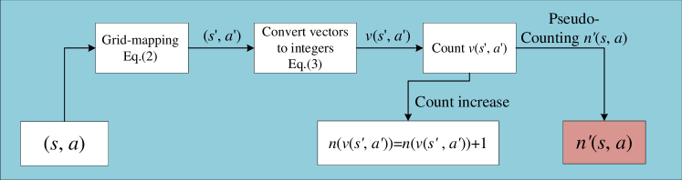
where and are respectively the dimensions of the action space and state space. In this way, counting is equivalent to counting the state-action pair corresponding to . The entire process of obtaining pseudo-counting through GPC can be seen in Figure 1.
Since GPC maintains the original data distribution to a certain extent, it can preserve the distribution characteristics of uncertainty in the state-action space and accurately quantify the uncertainty of different state-actions in various environments. Moreover, the approximation of the true state-action uncertainty in the case of continuous state-action space can be theoretically proven thanks to this characteristic. Notably, the states used in the training process are known due to the model-free method, thus it is feasible to directly count all possible states in the static dataset instead of gridding the state. Nevertheless, in this paper, the state is gridded to save computational space.
4.2 Connection Between Pseudo-Count And Uncertainty
In continuous space, it is impossible to directly count the selection times of a certain state-action to obtain the uncertainty constraint. Therefore, the pseudo-count is generally used to approximate the real count to obtain the uncertainty constraint. The current methods need to assume that can approximate , which is hard to confirm, to prove that the method approximates the real uncertainty. To this end, Grid-Mapping Pseudo-Count(GPC) is proposed in this paper to reduce the preconditions, as it can obtain a reasonable uncertainty constraint without preconditions. To prove that the GPC can obtain appropriate uncertainty constraints in continuous space, we first need to prove that the count-based method can obtain appropriate uncertainty constraints in discrete space.
Lemma 1 (Hoeffding’s inequality).
Let be independent random variables, and . The empirical mean of the random variable is expressed as:
Then Hoeffding’s theorem states that:
| (4) |
The proof is referred to hoeffding1994probability . Under the condition of Lemma 4 we can get:
Corollary 1.
is a suitable uncertain constraint in offline RL.
From the above corollary, it can be inferred that in discrete space, GPC can obtain appropriate uncertainty constraints. We extend the results of discrete spaces to continuous spaces. In the following part, the reasonability of the uncertainty constraint obtained by GPC for continuous spaces will be proved.
For continuous spaces, we consider the epistemic uncertainty. To prove that GPC can obtain an approximation of the epistemic uncertainty constraint. Firstly we attempt to obtain an approximation of the epistemic uncertainty constraint. Secondly, we prove that the uncertainty obtained by GPC is equivalent to the approximation of the epistemic uncertainty constraint.
Referring to the work of pioneers, an approximation of the uncertainty constraint can be obtained by the following process. First, the definition of the linear MDP is given wang2020reward and the corresponding assumptions about the considered MDP is made as follows.
Definition 1.
An MDP is linear if it satisfies that the state transition function and reward function are linear to the transition kernel function .
Although the linear hypothesis seems to be very strict, actually as the expression of the transition kernel of state and action is unlimited, the assumption of linear MDP has a very strong expression ability.
Definition 2.
is a suitable epistemic uncertainty function if it satisfies the following equation:
| (5) |
where is the Bellman equation, is the empirical Bellman equation estimated through the static datasets.
Definition 2 is just a common definition for determining whether uncertainty is appropriate. From Definition 1 and Definition 2, we can obtain a quantification of epistemic uncertainty.
Lemma 2.
In linear MDP, the reward function and transition kernel assumptions are linear to the representation of state-actions . When selecting appropriate , the following lower confidence limit penalty is an appropriate uncertainty quantification:
| (6) |
where .
The explanation of Eq(6) can be found in jin2020provably ; abbasi2011improved . By substituting Eq(6) into Eq(5) to get:
| (7) |
Under the above conditions, we give the corollary.
Corollary 2.
In linear MDPs, can be regarded as a continuous function. That is, the uncertainty in continuous offline RL can be approximated by a continuous function.
Although it is difficult to prove that is a continuous function for all , it is true for all the commonly used kernel functions. A detailed description is given in Appendix 5.
Based on the above conditions, Theorem 1 is inferred as follows:
Theorem 1.
In a continuous linear MDP, when the state space and action space are not unlimited. For the uncertainty constraint obtained by GPC, there exists a constant such that for any has:
Proof.
When the state-action space is gridded using the Grid-Mapping method, the number of times that all state-action pairs in the region are selected is exploited to approximate the uncertainty of any point in it, using to represent the uncertainty obtained by this method. From Corollary 1, it can be obtained that:
| (8) |
where
and because at any , then from the Mean value theorems for definite integrals, it can be obtained that :
| (9) |
where is a point in the interval . Then, by substituting Eq(8) into Eq(7), it can be inferred that
| (10) |
That is, the uncertainty is equal to the estimated uncertainty obtained by the interval where is located in. Since is continuous, when the interval is taken as small enough, it can be inferred that:
| (11) |
Therefore, for the uncertainty in any , it can be estimated using the corresponding . Finally, since is proved to be continuous and an appropriate uncertainty quantization, it can replace above. Substitute Eq(10) into Eq(6) to obtain:
| (12) |
That is, an appropriate uncertainty constraint can be obtained by GPC. ∎
4.3 Agent Learning With Uncertainty
Since the uncertainty is quantified, it is used to update the Q-function by constraint OOD samples. OOD samples that are sate-actions used in the training but are not covered by the static dataset and the Q-function approximator may give inaccurate Q-values estimations for these samples. Agents may utilize some sub-optimal samples brought by inaccurate estimations, leading to poor performance. Due to this, we use the quantified uncertainty to constrain them. we divide the loss function is divided into two parts: in-distribution loss and OOD loss. The OOD loss is the loss function of OOD actions obtained by the quantified uncertainty. The in-distribution loss is the conventional TD-error determined by the Bellman operator, which has the same form as the naive SAC and can be obtained as follows:
| (13) |
| (14) |
where is the -th target Q-network, is the corresponding result of the -th Q-network. For the OOD loss, the target Q-values of OOD samples are formulated as follows:
| (15) | ||||
In this equation, and are hyperparameters for adjusting the degree of constraint, is is represents an OOD state-action pair obtained by a sample in the dataset according to policy . Here and have the same state, but and may be different.
Since the Q-value of the OOD sample is generated by the Q-function, its pessimistic estimate is obtained by subtracting the uncertainty from itself. In addition, the Q-values of OOD samples are limited by in the proposed algorithm to make the training more stable. Similar to , the OOD loss is calculated as follows:
| (16) |
Finally, the loss function is expressed as the sum of the OOD loss and the in-distribution loss as follows:
| (17) |
Besides, the policy is then updated by the constrained rather than the usual Q-function for avoiding the overestimated state-actions being chosen, thus making it more inclined to learn a conservative policy. The updated expression is as follows:
| (18) |
Here, is a hyperparameter. The proposed algorithm is trained by updating the Q-function and the policy by the above methods. In the early stage of training, the large uncertainty makes the Q-function have a pessimistic estimate of the Q-value of the OOD sample, thus the agent tends to select the existing state-action pairs. In the middle and later stages of training, as the uncertainty decreases, the samples that are outside the dataset but may perform well are likely to be chosen by the policy, leading to a balance between conservatism and exploration.
Input: Initial policy parameter ; Q-function parameters ,; Target Q-function parameters, ; offline dataset ; The number of times the data is selected .
Output: Trained policy
4.4 Proposed Algorithm GPC-SAC
To demonstrate the effectiveness of the proposed method, SAC is employed as the benchmark algorithm in experiments and is combined with the proposed GPC as a novel algorithm called GPC-SAC. The differences between GPC-SAC and SAC are illustrated in Section 4.1 and 4.3. The specific implementation of the pseudo-code of GPC-SAC is shown as algorithm 1.
GPC-SAC uses the uncertainty obtained by GPC to constrain the Q-value and uses the constrained Q-value to guide the agent to improve its policy. This operation theoretically takes a short time and can improve the performance of SAC. In order to verify the effect of GPC-SAC, we carried out experiments on D4RL dataset.
5 Experiment
| Environment | IQL | UWAC | CQL | PBRL | TD3-CVAE | GPC-SAC |
|---|---|---|---|---|---|---|
| halfcheetah-medium | ||||||
| hopper-medium | ||||||
| walker2d-medium | ||||||
| halfcheetah-medium-replay | ||||||
| hopper-medium-replay | ||||||
| walker2d-medium-replay | ||||||
| halfcheetah-medium-expert | ||||||
| hopper-medium-expert | ||||||
| walker2d-medium-expert | ||||||
| halfcheetah-expert | — | |||||
| hopper-expert | — | |||||
| walker2d-expert | — | |||||
| Average |
5.1 Experiment Setting
To demonstrate the effectiveness and rationality of GPC-SAC, experiments are performed in the popular D4RL Benchmark fu2020d4rl for different continuous control tasks, compared with some extensively studied baseline algorithms and current SOTA algorithms. The D4RL dataset is composed of three types of environments: halfcheetah, hopper and walker2d. Each type of environment uses random, medium, medium-replay, medium-expert and expert five different policies to collect samples. Random means completely random sampling to obtain data. Medium means first training an algorithm online, stopping training in the middle, and then using this partially trained strategy to collect sample data. Medium-replay means training an algorithm online until the policy reaches a medium performance level and then collecting all samples saved in the buffer during training. Medium-expert means mixing the same amount of expert policy and data collected by medium policy. Expert means training a policy online to reach the expert performance level and collecting sample data using this expert policy. For halfcheetah and walker2d environments, we train 1000 episodes, and for the hopper environment, we train 3000 episodes. Each episode performs 1000 steps of training and uses 5 different random seeds for each test environment for testing. For more detailed parameter settings, please refer to Appendix A.3.
In environments of medium, medium-replay, medium-expert and expert, GPC-SAC is compared with several classic algorithms and SOTA algorithms. The involved algorithms are: IQL Kostrikov2021OfflineRL , which proposed an in-sample Q-learning algorithm that does not use OOD samples at all, UWAC wu2021uncertainty , an uncertainty estimation algorithm that improves bear through dropout, CQL kumar2020conservative , an algorithm that constrains the strategy by conservatively estimating the Q-value of OOD samples through regularization terms, TD3-CVAE rezaeifar2022offline , another model-free domain algorithm that uses the count-based method to subtract the predicted uncertainty from the reward for conservative learning, and PBRL bai2022pessimistic , an algorithm in the model-free field that quantifies uncertainty and constraints Q-values through the ensemble method.
5.2 Experiment Result
5.2.1 Result analysis
From Table 1, it can be seen that GPC-SAC has the best performance in most environments. Comparing GPC-SAC with other algorithms. In halfcheetah-medium and halfcheetah-expert, GPC-SAC outperforms the highest-performing algorithm 20%. In halcheetah-medium-expert, although GPC-SAC has a relatively poor performance, compared with the best-performing PBRL, the performance of GPC-SAC is only 5% lower than that of PBRL. In general, compared GPC-SAC with classic algorithms and SOTA algorithms, only PBRL has approximate performance, but the computational cost of PBRL is much larger than GPC-SAC, it can be seen in Table 2. The experiment shows the effectiveness of the uncertainty constraint method, and GPC can obtain reasonable uncertainty constraints through simple calculations.
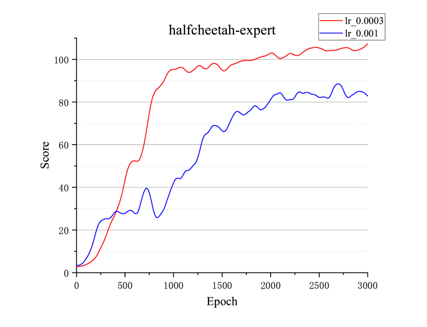
In addition to the experimental results in Table 1, we also compare the training curves of various algorithms, training curves of walker2d-medium-replay and halfcheetah-expert are shown in Figure 1. In halfcheetah-expert, CQL and PBRL that constrain the Q-value cannot find a not bad policy within 1500 epochs, both CQL and PBRL require 3000 epochs of training to find an optimal policy. While GPC-SAC can find a perform well policy within 1500 epochs. From the training curve of walker2d-medium-replay, it can be seen that GPC-SAC not only has the best performance but also the second-best in stability and training speed. The training curves of other environments can be seen in Appendix C.3.
5.2.2 Computational cost
In addition to comparing performance, we compared the computational time and computational space of GPC-SAC with PBRL, SAC and CQL which constrain Q-values. In the experiment, the number of ensembles used in PBRL is 10, which is consistent with the usage in the original paper. We ran a comparative experiment on a single NVIDIA GeForce RTX 3090, comparing the time and space of training for one epoch. The comparison results can be seen in Table 2.
| Algorithm | Runtime(s) | GPU Memory(GB) |
|---|---|---|
| SAC | 42.1 | 1.3 |
| CQL | 58.8 | 1.4 |
| PBRL | 178.9 | 1.8 |
| GPC-SAC | 47.7 | 1.3 |
From Table 2, it can be seen that GPC-SAC only increases a small amount of training time and operation space compared with SAC. Compared with PBRL using ensemble method quantization uncertainty and CQL using regularization constraints, GPC-SAC using GPC has shorter training time and lower computational space. This is because PBRL requires additional training of multiple networks; CQL requires multiple gradient computations brought by additional regularization. But GPC-SAC only needs the simple parallel operation of discretizing action space, so it has less computational cost.
6 Conclusions
In this paper, we first propose GPC, a method that utilizes pseudo-counting to quantify uncertainty in offline RL. We theoretically prove that GPC can obtain accurate uncertainty constraints under fewer conditions. Secondly, we propose GPC-SAC, a model-free offline RL algorithm for continuous environments by constraining the Q-value using GPC. In experiments, our experimental results on the D4RL dataset show that GPC-SAC has better performance and less computational costs than advanced model-free offline reinforcement learning algorithms. Both theoretical and experimental results show that our algorithm has the most advanced effect.
References
- (1) OpenAI, “Gpt-4 technical report,” 2023.
- (2) O. Vinyals, I. Babuschkin, W. M. Czarnecki, M. Mathieu, A. Dudzik, J. Chung, D. H. Choi, R. Powell, T. Ewalds, P. Georgiev, J. Oh, D. Horgan, M. Kroiss, I. Danihelka, A. Huang, L. Sifre, T. Cai, J. P. Agapiou, M. Jaderberg, A. S. Vezhnevets, R. Leblond, T. Pohlen, V. Dalibard, D. Budden, Y. Sulsky, J. Molloy, T. L. Paine, C. Gulcehre, Z. Wang, T. Pfaff, Y. Wu, R. Ring, D. Yogatama, D. Wünsch, K. McKinney, O. Smith, T. Schaul, T. Lillicrap, K. Kavukcuoglu, D. Hassabis, C. Apps, and D. Silver, “Grandmaster level in starcraft ii using multi-agent reinforcement learning,” Nature, vol. 575, no. 7782, pp. 350–354, 2019.
- (3) E. Kaufmann, L. Bauersfeld, A. Loquercio, M. Mller, V. Koltun, and D. Scaramuzza, “Champion-level drone racing using deep reinforcement learning,” Nature, vol. 620, no. 7976, pp. 982–987, 2023.
- (4) C. Yu, J. Liu, and S. Nemati, “Reinforcement learning in healthcare: A survey,” ACM Computing Surveys (CSUR), vol. 55, no. 1, pp. 1–36, 2021.
- (5) R. S. Sutton and A. G. Barto, Reinforcement learning: An introduction. MIT press, 2018.
- (6) S. Levine, A. Kumar, G. Tucker, and J. Fu, “Offline reinforcement learning: Tutorial, review, and perspectives on open problems,” arXiv preprint arXiv:2005.01643, 2020.
- (7) S. Fujimoto, D. Meger, and D. Precup, “Off-policy deep reinforcement learning without exploration,” in International conference on machine learning. PMLR, 2019, pp. 2052–2062.
- (8) R. Agarwal, D. Schuurmans, and M. Norouzi, “An optimistic perspective on offline reinforcement learning,” in International Conference on Machine Learning. PMLR, 2020, pp. 104–114.
- (9) R. F. Prudencio, M. R. O. A. Maximo, and E. L. Colombini, “A survey on offline reinforcement learning: Taxonomy, review, and open problems,” IEEE Transactions on Neural Networks and Learning Systems, 2023.
- (10) A. Kumar, J. Fu, M. Soh, G. Tucker, and S. Levine, “Stabilizing off-policy q-learning via bootstrapping error reduction,” Advances in Neural Information Processing Systems, vol. 32, 2019.
- (11) A. Kumar, A. Zhou, G. Tucker, and S. Levine, “Conservative q-learning for offline reinforcement learning,” Advances in Neural Information Processing Systems, vol. 33, pp. 1179–1191, 2020.
- (12) C. Bai, L. Wang, Z. Yang, Z. Deng, A. Garg, P. Liu, and Z. Wang, “Pessimistic bootstrapping for uncertainty-driven offline reinforcement learning,” arXiv preprint arXiv:2202.11566, 2022.
- (13) C. Gulcehre, Z. Wang, A. Novikov, T. L. Paine, S. G. Colmenarejo, K. Zolna, R. Agarwal, J. Merel, D. Mankowitz, C. Paduraru, G. Dulac-Arnold, J. Li, M. Norouzi, M. Hoffman, O. Nachum, G. Tucker, N. Heess, and N. de Freitas, “Rl unplugged: A suite of benchmarks for offline reinforcement learning,” Advances in Neural Information Processing Systems, vol. 33, pp. 7248–7259, 2020.
- (14) I. Osband, J. Aslanides, and A. Cassirer, “Randomized prior functions for deep reinforcement learning,” Advances in Neural Information Processing Systems, vol. 31, 2018.
- (15) S. Rezaeifar, R. Dadashi, N. Vieillard, L. Hussenot, O. Bachem, O. Pietquin, and M. Geist, “Offline reinforcement learning as anti-exploration,” in Proceedings of the AAAI Conference on Artificial Intelligence, vol. 36, no. 7, 2022, pp. 8106–8114.
- (16) J. Hong, A. Kumar, and S. Levine, “Confidence-conditioned value functions for offline reinforcement learning,” arXiv preprint arXiv:2212.04607, 2022.
- (17) J. Fu, A. Kumar, O. Nachum, G. Tucker, and S. Levine, “D4rl: Datasets for deep data-driven reinforcement learning,” arXiv preprint arXiv:2004.07219, 2020.
- (18) T. Haarnoja, A. Zhou, P. Abbeel, and S. Levine, “Soft actor-critic: Off-policy maximum entropy deep reinforcement learning with a stochastic actor,” in International conference on machine learning. PMLR, 2018, pp. 1861–1870.
- (19) V. Mnih, K. Kavukcuoglu, D. Silver, A. A. Rusu, J. Veness, M. G. Bellemare, A. Graves, M. Riedmiller, A. K. Fidjeland, G. Ostrovski, S. Petersen, C. Beattie, A. Sadik, I. Antonoglou, H. King, D. Kumaran, D. Wierstra, S. Legg, and D. Hassabis, “Human-level control through deep reinforcement learning,” nature, vol. 518, no. 7540, pp. 529–533, 2015.
- (20) C.-J. Hoel, T. Tram, and J. Sjöberg, “Reinforcement learning with uncertainty estimation for tactical decision-making in intersections,” in 2020 IEEE 23rd international conference on intelligent transportation systems (ITSC). IEEE, 2020, pp. 1–7.
- (21) W. R. Clements, B. V. Delft, B.-M. Robaglia, R. B. Slaoui, and S. Toth, “Estimating risk and uncertainty in deep reinforcement learning,” arXiv preprint arXiv:1905.09638, 2019.
- (22) M. Janner, J. Fu, M. Zhang, and S. Levine, “When to trust your model: Model-based policy optimization,” Advances in neural information processing systems, vol. 32, 2019.
- (23) T. Yu, G. Thomas, L. Yu, S. Ermon, J. Zou, S. Levine, C. Finn, and T. Ma, “Mopo: Model-based offline policy optimization,” Advances in Neural Information Processing Systems, vol. 33, pp. 14 129–14 142, 2020.
- (24) T. Yu, A. Kumar, R. Rafailov, A. Rajeswaran, S. Levine, and C. Fin, “Combo: Conservative offline model-based policy optimization,” Advances in neural information processing systems, vol. 34, pp. 28 954–28 967, 2021.
- (25) V. Mai, K. Mani, and L. Paull, “Sample efficient deep reinforcement learning via uncertainty estimation,” arXiv preprint arXiv:2201.01666, 2022.
- (26) M. G. Bellemare, S. Srinivasan, G. Ostrovski, T. Schaul, D. Saxton, and R. Munos, “Unifying count-based exploration and intrinsic motivation,” Advances in neural information processing systems, vol. 29, 2016.
- (27) A. Agarwal, S. Kakade, A. Krishnamurthy, and W. Sun, “Flambe: Structural complexity and representation learning of low rank mdps,” Advances in neural information processing systems, vol. 33, pp. 20 095–20 107, 2020.
- (28) R. T. McAllister and C. E. Rasmussen, “Improving pilco with bayesian neural network dynamics models,” in Data-efficient machine learning workshop, ICML, vol. 4, no. 34, 2016, p. 25.
- (29) Y. J. Ma, A. Shen, O. Bastani, and D. Jayaraman, “Conservative and adaptive penalty for model-based safe reinforcement learning,” in Proceedings of the AAAI conference on artificial intelligence, vol. 36, no. 5, 2022, pp. 5404–5412.
- (30) Z. Zhu, E. Bıyık, and D. Sadigh, “Multi-agent safe planning with gaussian processes,” in 2020 IEEE/RSJ International Conference on Intelligent Robots and Systems (IROS). IEEE, 2020, pp. 6260–6267.
- (31) R. Kidambi, A. Rajeswaran, P. Netrapalli, and T. Joachims, “Morel: Model-based offline reinforcement learning,” Advances in neural information processing systems, vol. 33, pp. 21 810–21 823, 2020.
- (32) Y. Wu, S. Zhai, N. Srivastava, J. Susskind, J. Zhang, R. Salakhutdinov, and H. Goh, “Uncertainty weighted actor-critic for offline reinforcement learning,” arXiv preprint arXiv:2105.08140, 2021.
- (33) G. An, S. Moon, J.-H. Kim, and H. O. Song, “Uncertainty-based offline reinforcement learning with diversified q-ensemble,” Advances in neural information processing systems, vol. 34, pp. 7436–7447, 2021.
- (34) G. Ostrovski, M. G. Bellemare, A. Oord, and R. Munos, “Count-based exploration with neural density models,” in International conference on machine learning. PMLR, 2017, pp. 2721–2730.
- (35) H. Tang, R. Houthooft, D. Foote, A. Stooke, X. Chen, Y. Duan, J. Schulman, F. D. Turck, and P. Abbeel, “# exploration: A study of count-based exploration for deep reinforcement learning,” Advances in neural information processing systems, vol. 30, 2017.
- (36) J. Choi, Y. Guo, M. Moczulski, J. Oh, N. Wu, M. Norouzi, and H. Lee, “Contingency-aware exploration in reinforcement learning,” arXiv preprint arXiv:1811.01483, 2018.
- (37) W. Hoeffding, “Probability inequalities for sums of bounded random variables,” The collected works of Wassily Hoeffding, pp. 409–426, 1994.
- (38) C. Jin, Z. Yang, Z. Wang, and M. I. Jordan, “Provably efficient reinforcement learning with linear function approximation,” in Conference on Learning Theory. PMLR, 2020, pp. 2137–2143.
- (39) R. Wang, S. S. Du, L. Yang, and R. R. Salakhutdinov, “On reward-free reinforcement learning with linear function approximation,” Advances in neural information processing systems, vol. 33, pp. 17 816–17 826, 2020.
- (40) Y. Abbasi-Yadkori, D. Pál, and C. Szepesvári, “Improved algorithms for linear stochastic bandits,” Advances in neural information processing systems, vol. 24, 2011.
- (41) I. Kostrikov, A. Nair, and S. Levine, “Offline reinforcement learning with implicit q-learning,” ArXiv, vol. abs/2110.06169, 2021.
- (42) Y. Gal, R. McAllister, and C. E. Rasmussen, “Improving pilco with bayesian neural network dynamics models,” in Data-efficient machine learning workshop, ICML, vol. 4, no. 34, 2016, p. 25.
7 Acknowledgments
This work was supported by the National Natural Science Foundation of China [grant numbers: 12201656], Science and Technology Projects in Guangzhou [grant numbers: SL2024A04J01579] and Key Laboratory of Information Systems Engineering (CN).
Appendix A Algorithm Implementation
A.1 Implementation Details
In the experiment, our handling of state space and action space is different. Since the selection of states in model-free offline RL is limited to the existing states in the static dataset, the selection of states is independent of the entire training process, so we do not need to gridding states in each training, but directly store the grid-mapped values corresponding to each state. Therefore, we only need to deal with the actions during each training session.
Our method maps each dimension of the state space and action space separately. In order to prevent algorithm failure caused by the non-existent of Eq(2) due to the static dataset having only one possible value in a certain dimension. For state, we first compute whether to map that dimension before training. This processing can also reduce the computational space used. For action, we use to prevent algorithm failure.
A.2 Grid-Mapping Implementation Details
For the use of grid-mapping, We propose Eq(2) and choose . Because during training, the integer corresponding to one state-action may be equivalent to the integer corresponding to another state-action. For example, for a two-dimensional state-action space, using , it can be seen from Eq(3) that
This means an OOD state-action corresponding to the vector (1,-1) is equivalent to another unrelated state-action in the dataset corresponding to vector (0,1). This relationship may lead to an overestimation of the Q-value of some OOD state-actions during training. As (0,1) has already accumulated enough visits, resulting in smaller uncertainty constraints for the state-action corresponding to (1,-1). When selecting the state-action corresponding to (1,-1) during training, it leads to an overestimation of the Q-value of (1,-1), which may hurt the training results.
To reduce the impact of such errors, Eq(2) can be used to consider OOD state-actions that are closer to the state-actions in the dataset. The use of Eq(2) ensures that the probability of the policy selecting an overestimated state-action is as small as possible. The specific proof can be seen in the theorem section, and the following is an example to illustrate this method.
Choosing a two-dimensional space with and as an example, where after gridding are the state-actions within the dataset. In this situation it has
| (19) |
So, for these , while , it have or . As the policy is learned from static datasets, the state-actions such as (2,6), (0,-4) that are far away from the static dataset will hardly be selected. The state-actions closer to the static dataset are more likely to be selected which have the same properties likes sate-actions in the dataset. This method can ensure that or the corresponding has a sufficiently low probability of being selected by the policy, so this method can effectively reduce the impact of error. The proof can be seen in Theorem B.4.
Although Grid-mapping with and theoretically has better performance than and , but some hyperparameters also need to be adjusted due to them. Therefore, we did not conduct too much testing on parameters and . Interested readers can conduct experiments on the code we provide.
A.3 Hyperparameter
The specific implementation of GPC-SAC can be found at https://github.com/lastTarnished/GPC-SAC. We conducted experiments on the latest v2 dataset of D4RL, which can be publicly used at https://github.com/Farama-Foundation/D4RL. The following are the implementations of the comparative algorithms in our experiment. (1)For CQL, we referred to https://github.com/aviralkumar2907/CQL/tree/master which is the official implementation of CQL. (2)For the implementation of IQL, we refer to IQL https://github.com/ikostrikov/implicit_q_learning this code has simplified the implementation of IQL compared to the official code, resulting in a slight decrease in performance in a few environments. (3)For the implementation of PBRL, we refer to https://github.com/Baichenjia/PBRL and no changes were made to the core code.
| Hyperparameter | value |
|---|---|
| discount | 0.99 |
| policy_rl | 3e-4 |
| qf_rl | 3e-4 |
| soft_target_tau | 5e-3 |
| train_pre_loop | 1000 |
| Q-network | FC(256,256,256) |
| Optimizer | Adam |
| activation_function | relu |
| 1 | |
| 0.1 |
| Environment | k | epoch | |
|---|---|---|---|
| halfcheetah-medium | 5 | 2 | 1000 |
| hopper-medium | 18 | 4 | 3000 |
| walker2d-medium | 7 | 4 | 1000 |
| halfcheetah-medium-replay | 5 | 3 | 1000 |
| hopper-medium-replay | 15 | 3 | 3000 |
| walker2d-medium-replay | 7 | 3 | 1000 |
| halfcheetah-medium-expert | 5 | 3 | 1000 |
| hopper-medium-expert | 25 | 5 | 3000 |
| walker2d-medium-expert | 7 | 5 | 1000 |
| halfcheetah-expert | 7 | 6 | 3000 |
| hopper-expert | 25 | 5 | 3000 |
| walker2d-expert | 7 | 5 | 1000 |
GPC-SAC is modified from SAC, and most of the hyperparameters selection of GPC-SAC are followed to SAC. Compared to SAC, we have additionally introduced the number of partitions and in the state-action space for each dimension, uncertainty constraint parameter and uncertainty coefficient for these three hyperparameters. Table 3 shows the selection of hyperparameters that remain unchanged in each environment.
, and are the key hyperparameters for GPC-SAC, for general environment, we generally choose and collectively referred to as . We combine the dimensionality of the state-action space to choose and . When the selected is too large, it will slow down the training speed. And when is too small, it may affect the training results. Therefore, the selection of is crucial. determines whether we can get appropriate uncertainty constraints. When selecting appropriate , the count-based constraint method can approximate epistemic uncertainty.
For the hopper environment, the effective dimension of action space is 3 and the effective dimension of state space is 6. Due to the low dimension, we can use a larger , which we choose from 15, 18, and 25. For environments halfcheetah and walker2d, the effective dimension of action space is 6, and the effective dimension of state space is 17. We use a smaller to deal with them, our is selected from 5 and 7. For , we select this parameter based on the rewards of state-actions in each static dataset. Generally, we choose around the average reward in the static dataset. Table 4 shows the hyperparameter combinations we used in the experiment, but it is not necessarily the optimal combination of hyperparameters.
For parameters and , in addition to the above analysis, we also provide direct reference formulas. Although using specific parameters in some environments may achieve better results, using the parameters we provide can achieve good results. For parameter n as follows. For parameter , choose can be suitable values, where expressed the dimension of action space. For parameter , we mostly choose the integer closest to and the average values of the dataset. Although special parameters may yield better results, using the parameter selection method we provide can already yield good results. The selection of parameters within a certain range is not too sensitive. In the experiment, when the value of is between several integers close to the mean and , good results can be obtained. For , when we select that falls within the range we provided, good results can also be obtained. To verify the effectiveness of the above parameter ranges, we conducted ablation experiments in the last part.
Appendix B Proofs
B.1 Count-based Uncertainty
In this section, we supplement the proof of Corollary 1, that is, the rationality of count-based method in discrete space.
Since is an independent random variable in offline RL, can be substituted into Lemma 4 to obtain:
| (20) |
Select a probability that allows, it can be obtained from the above equation that , and then, from we can get . In the application of offline RL, we hope that the estimation of the Q-value will become more accurate as the number of training times increases. Therefore, we hope that the value of gradually decreases as the training progresses. For example, when T is used to represent the current training epoch, meets the above requirements. Use this p, we can get .
B.2 Uncertainty and
In this part, we use to obtain an uncertainty constraint, and we demonstrate the rationality of using as an uncertainty constraint.
We discuss this problem in tabular cases and general cases.
For finite tabular MDPs, in , parameter represents all selected state-actions in the static dataset. In this situation, we can get Lemma 3:
Lemma 3.
In tabular MDPs, the uncertainty can be approximated by the counts of each state-action using the following method:
| (21) |
Proof.
In tabular MDPs, we can define
| (27) |
where , value 1 at -th, all other positions in the vector are value 0. Which means that is a count of -th state-action . So we can compute that
| (28) |
The diagonal of the matrix represents the count of all possible state-actions in the tabular MDP. Then we can compute that
| (29) |
For general situations, the epistemic uncertainty in a state-action can be considered as the difference between the true Q-value and the estimated Q-value , which is
| (31) |
Due to the assumption of linear MDP, , both have a linear relationship with , just like
| (32) |
Where is the estimated parameter and is the actual parameter. For the parameter, is used to estimate the Q-value, since Q can be expressed as r and V by Bellman Equation, the value of can be obtained by minimizing the empirical Mean-Square Bellman-Error (MSBE) and regularization term as follows:
| (33) |
The explicit solution of can be calculated as:
| (34) |
so the epistemic uncertainty can be represented by , that is
| (35) |
In addition to the above analysis, we need Assumption 1.
Assumption 1.
The prior parameter known from the dataset and epistemic uncertainty satisfies
| (36) |
Under the condition of Assumption 1, the following lemma can be drawn:
Lemma 4.
Under Assumption 1, can approximate real uncertainty.
Proof.
can approximate real uncertainty, which means that
| (37) |
where
so we want to prove that
| (38) |
So we need to obtain . From Eq(35) we know that
| (39) |
Since satisfies normally distributed, we can obtain
| (40) |
From we know that
| (41) |
When using to denote the probability density function of the distribution. Using Bayes rule it has
| (42) |
Here, according to the probability density function of normal distribution, we can get:
| (43) |
| (44) |
so
| (45) |
From this equation, we know that
| (46) |
so for all ,
∎
Although the above theorem requires that both and satisfy normal distribution, it can be inferred from the above proof process that for distributions with additivity, this conclusion holds, that is, Lemma 2 also applies to partial distributions.
B.3 Continuity of
In this section, we add the proof of Lemma 2, which is why we consider as a continuous function.
To illustrate the continuity of , we directly calculate . For this, we first represent in the following form
| (47) |
where . Since is an invertible matrix, the inverse of matrix can be directly calculated as
| (48) |
where , are polynomials related to , , …, . We represent as . Then can be represented as
| (49) |
Plugging Eq(48) into Eq(49) get
| (50) |
From this equation, we can see that for kernel functions with continuous components, such as Gaussian kernel and other common kernel functions. is continuous, and since is reversible, so , and the composition of continuous functions is also a continuous function, then is also a continuous function. And is the composite of and , therefore it is also a continuous function.
Therefore, based on the above proof, we can obtain the following Theorem, from which we can know that Lemma 2 holds.
Theorem 2.
When the components of each dimension of kernel function are continuous, is also continuous.
B.4 Rational of GPC
Theorem 3.
Set be the probability was selected in a discrete state-action space. , it has the probability of selecting a state-action with the same corresponding integer as .
Proof.
We prove this conclusion with in a two-dimensional state-action space, and for high-dimensional spaces, it can be obtained by analogy. Since the states used in the training are only the existing states in the dataset, we can know
| (51) |
Therefore, take any possible , there are only different possible outcomes less than m satisfy so, , we want to prove
| (52) |
Where ,. Due to that state-actions are obtained by agent learning from a static dataset, the lower the selection rate of actions that deviate from existing actions in the dataset, we can write it as:
| (53) |
B.5 Policy optimization guarantee
In this section, we will prove that GPC-SAC can ensure the effectiveness of the policy will not decrease after each training in any environment. Our proof section refers to SAC. To prove the conclusion, we first provide some relevant definitions of the section. Likes SAC, the relationship between V and Q in GPC-SAC is that
| (55) |
is updated by
| (56) | ||||
For the policy obtained from each update, we represent it as
| (57) |
In this equation, is the current policy, is used to standardize the entire distribution. Although is generally difficult to handle, it does not contribute to the gradient of the new policy , so it can be ignored. After representing as the above form, we can obtain the following theorem.
Theorem 4.
Let be the policy obtained from the current epoch training, is the new policy optimized by Eq(57), then it have for all . Here .
Proof.
In Eq(57)
| (58) | |||
so
| (59) | ||||
Because expanding the KL divergence can get
| (60) |
And since for , even in the worst case, we can choose . So it has
| (61) | |||
Since only depends on the state, we can simplify the above equation as
| (62) | |||
Substituting Eq(55) into the above equation we can know that
| (63) |
Appendix C Experiment
C.1 Experiment in Maze2d environemnts
One advantage of GPC-SAC is its ability to handle complex problems in low-dimensional situations. To demonstrate the advantage of GPC-SAC, we conducted experiments on mze2d environments. Maze2D is a maze navigation task, the purpose of maze2d is to test the ability of offline RL algorithm to connect suboptimal trajectories to find the shortest path to the target point. Maze2d includes three types of mazes, from easy to difficult: umaze, medium and large. Table 5 are the training results of GPC-SAC and some sota algorithms in maze2d. It can be seen that GPC-SAC performs astonishingly in all tasks of maze2d, especially in maze2d-large. All other algorithms we know can not reach 65 scores. GPC-SAC can achieve xxx points, which far exceeds the current sota algorithms.
| Environment | CQL | IQL | PBRL | GPC-SAC |
|---|---|---|---|---|
| maze2d-umaze | 56.3 | 46.9 | 86.7 | 141.0 |
| maze2d-medium | 24.8 | 32.0 | 71.1 | 103.7 |
| maze2d-large | 15.3 | 64.2 | 64.5 | 134.3 |
| pen-expert | 107.0 | 117.2 | 137.7 | 118.8 |
| hammer-expert | 86.7 | 124.1 | 127.5 | 95.6 |
| door-expert | 101.5 | 105.2 | 95.7 | 101.0 |
| average | 65.3 | 81.6 | 97.2 | 115.7 |
C.2 Experiment in adroit environments
The shortcoming of count-based methods is that as the state-action space increases, the possible state-actions exponentially increase. Currently, most count-based algorithms are unable to address this issue well. The advantage of GPC-SAC compared to other count-based algorithms is that it can consider state space and action space separately. For the problem of large action dimension, GPC-SAC is not affected by it as it only requires states within the dataset. For the problem of large state dimension, as the amount of data in static datasets is limited, it will not affect GPC-SAC. For the problem of large action dimension, We are currently solving this problem by reducing the number of action space partitions . The Adroit environment is a series of more complex environments compared to the Gym environment, and the action dimensions of the Adroit environment are all over 20 dimensions. Therefore, it is a huge challenge for count-based methods. So we conducted experiments in adroit environments to demonstrate that GPC-SAC can solve high-dimensional problems to a certain extent. We show the experiment results in Table 5. The hyperparameters of GPC-SAC in maze2d and adroit are shown in Table 6.
It can be seen that although the count-based methods have difficulty solving high-dimensional problems, GPC-SAC can also have good results in adroit environments. But we have to admit that GPC-SAC is difficult to deal with environments where the dimension of action space is larger than 30.
| Environment | (state) | (action) | |
|---|---|---|---|
| maze2d-umaze | 30 | 30 | 0.2 |
| maze2d-medium | 30 | 30 | 0.2 |
| maze2d-larger | 30 | 30 | 0.2 |
| pen-expert | 1 | 0.6 | 30 |
| door-expert | 1 | 0.5 | 70 |
| hammer-expert | 1 | 0.5 | 15 |
C.3 Algorithm Comparison Experiment
In each environment, we compare the training curves of GPC-SAC, IQL and CQL, as shown in Figure LABEL:exp.
C.4 Ablation Experiment
For some parameters, we conducted ablation experiments to demonstrate the effectiveness of these parameters. The setting of ablation experiments is similar to that of the comparative experiment. We keep the remaining parameters unchanged and only change the parameters that need to be compared. The following are the settings and results of the ablation experiment.
Learning rate: The implementation of CQL in SAC framework and SAC itself use two different sets of Q-function learning rates, policy function learning rate and soft update rate. We compare two different parameters to choose the appropriate one. The experimental results are in Figure 16.
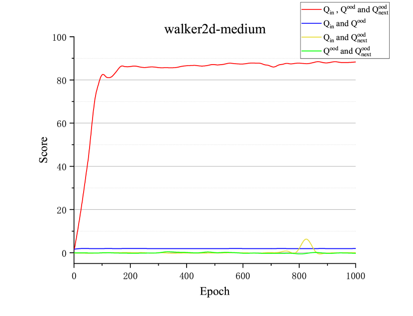
Application of OOD sample: We used , , and to update the Q-function together in the update. Theoretically, the use of each type of Q-value can be divided into seven types. We consider using three parts at the same time, using , using , and using four situations. The experimental results are in Figure 16. We have not conducted ablation experiments for the case of using only one type of Q, but the case of using only one type of Q can be obtained by analogy from the above results.
Uncertainty parameter for : The difference between and is that does not have known actions in the dataset to guide the agent’s actions. When using large uncertainty constraints on , the agent can still select in the static dataset, ensuring that the value of is not excessively underestimated. However, if the same uncertainty constraint is chosen for , it may lead to an excessive underestimation of the value of and , causing the agent misses some states and actions with high potentially, resulting in a decrease in algorithm performance. Therefore, we conducted ablation experiments on parameter , selecting from {0,0.1,1}, which respectively indicate not imposing constraints to at all, imposing smaller constraints to , and imposing equal constraints to and . The results of the experiment are shown in Figure LABEL:beta.
Sensitivity of parameters and : GPC-SAC introduces two key hyperparameters and . An important question is whether the selection of and will seriously affect the performance of GPC-SAC. Therefore, we conducted ablation experiments on and separately, we do ablation experiments on halfcheetah-medium for that medium-type environments may be more affected by parameters compared to others. We selected and with significant differences for comparison. It can be seen from FigureLABEL:beta_and_k that when using parameters within a certain range, good results can be obtained.