Heterogeneous Treatment Effects and
Causal Mechanisms

Abstract

The credibility revolution advances the use of research designs that permit identification and estimation of causal effects. However, understanding which mechanisms produce measured causal effects remains a challenge. A dominant current approach to the quantitative evaluation of mechanisms relies on the detection of heterogeneous treatment effects with respect to pre-treatment covariates. This paper develops a framework to understand when the existence of such heterogeneous treatment effects can support inferences about the activation of a mechanism. We show first that this design cannot provide evidence of mechanism activation without additional, generally implicit, assumptions. Further, even when these assumptions are satisfied, if a measured outcome is produced by a non-linear transformation of a directly-affected outcome of theoretical interest, heterogeneous treatment effects are not informative of mechanism activation. We provide novel guidance for interpretation and research design in light of these findings.

The credibility revolution in empirical social science has motivated the largescale adoption of research designs that facilitate unbiased estimation of causal effects (Samii, 2016; Angrist and Pischke, 2010). Such unbiased estimates allow for valid measurement of the effect of a treatment on an outcome. However, they do not generally provide evidence about why or how the treatment affected the outcome. These questions of why or how are ultimately questions about the activation and influence of causal mechanisms. Understanding the mechanisms that produce causal effects is central to our ability to use empirical evidence to understand social phenomena (Slough and Tyson, 2023a).

Applied researchers typically pursue a number of different approaches to ascertaining the mechanisms that generate causal effects. There exist at least four distinct approaches in the applied literature: (1) evaluation of the sign of treatment effects on a given outcome (e.g., Ashworth, Berry, and de Mesquita, 2023); (2) mediation analysis (Imai, Keele, and Tingley, 2010; Imai et al., 2011; Glynn, 2012; Imai and Yamamoto, 2013); (3) multimethod research involving some form of qualitative or quantitative triangulation of causal findings (Levy Paluck, 2010; Dunning, 2012); and (4) the estimation of heterogeneous treatment effects (HTEs). The last approach—HTEs—compares estimated treatment effects for various subgroups thought to be informative about mechanism activation. While this is currently the modal approach to (quantitative) mechanism-testing in political science, the theoretical properties of this enterprise are not well explored.

To examine the prevalence of the use of HTEs to learn about causal mechanisms, we survey the 2021 volumes of three leading journals in political science: the American Journal of Political Science (AJPS), the American Political Science Review (APSR), and the Journal of Politics (JoP). We first identify the subset of papers that analyze quantitative empirical data. We then report the proportion of those empirical papers that report HTEs or subgroup-specific treatment effects. Finally, we report the proportion of papers using HTEs that interpret these quantities as providing information about causal mechanisms(s). Table 1 shows that in each of the three leading journals, a majority of quantitative studies estimate HTEs. Moreover, conditional on reporting any HTEs, the vast majority of articles (82% across three journals) interpret these quantities as providing information about mechanisms. Collectively, these figures indicate that almost half (46%) of recent quantitative empirical articles in these journals use HTEs to assess mechanisms. Table A.1 further documents that the share of studies that use of HTE for mechanism detection is similar across all quantitative research designs/identification strategies in common usage.

	Number of articles:			Pr(Report HTEs $\mid$	Pr(Mechanism test $\mid$
Journal (Volume)	Total	Quant. empirical	Reporting HTEs	Quant. empirical)	Report HTE)
AJPS (65)	61	41	24	0.59	0.83
APSR (115)	102	75	42	0.56	0.90
JoP (83)	142	106	59	0.56	0.76
Total	305	222	125	0.56	0.82

Table 1: Authors’ classification of articles published in three leading political science journals in 2021.

Existing concerns about HTEs have largely focused on the statistical properties of relevant estimators and hypothesis tests. In particular, interaction effects are known to have low statistical power (e.g., McClelland and Judd, 1993). Moreover, estimation of HTEs with respect to many (pre-treatment) covariates risks multiple comparisons problems (Gerber and Green, 2012; Lee and Shaikh, 2014; Fink, McConnell, and Vollmer, 2014). While these criticisms are important, they are distinct from theoretical questions about how the presence or absence of HTEs links to causal mechanisms. We take on this challenge by asking: under what conditions do HTEs provide evidence of mechanism activation?

To answer this question, we develop a framework to formally link HTEs with respect to a covariate to the effect of a specific mechanism. To do so, we extend the workhorse causal mediation framework (Imai, Keele, and Tingley, 2010). Within our framework, a mechanism is an underlying process that influences experience in order to produce a (causal) effect if it is activated (Slough and Tyson, 2023a). A mediator, or mechanism representation, should thus be affected by treatment and have a non-zero (indirect) effect on the outcome if the mechanism is active for some unit. In order to use HTEs to detect mechanisms, empiricists rely on a measured moderator or pre-treatment covariate that is thought to predict the degree to which treatment activates a mechanism and/or the mechanism’s effect on an outcome of interest. Our results characterize the conditions under which heterogeneity in conditional average treatment effects (CATEs) with respect to a given moderator is a sufficient condition to show that the mechanism is active. A mechanism is active when its indirect effect is non-zero for some unit.

We first present two classes of exclusion assumptions that link HTEs to a specified mechanism. These assumptions hold that the moderator of interest is excluded with respect to (1) the average indirect effect of other mechanisms and (2) the average direct effect of the treatment on the outcome. The intuition for these assumptions is straightforward. The use of HTEs to assess the activation of a given mechanism relies on the additive separability of the effect of that mechanism from the effects of other mechanisms. These exclusion assumptions are needed to ensure that additive separability is possible. In their absence, the relationship between HTEs and the indirect effect of a mechanism is unspecified. In this sense, these assumptions are implicitly invoked by current practice, but are not explicitly stated or defended.

When these exclusion assumptions hold, what can we learn about a mechanism of interest from HTEs with respect to a given covariate? Our main results characterize what we can learn from the existence or non-existence of HTEs. We show that whether such learning is possible depends on the relationship between measured outcomes and the theory. We thus distinguish between outcome variables that are theorized to be directly affected by a mechanism versus (causally) subsequent outcomes that are indirectly affected.

First, consider the case in which a measured outcome is directly affected by the mechanism of interest. We show that when both exclusion assumptions hold, the existence of HTEs provides evidence of mechanism activation. This broadly conforms to current practices in applied research, albeit while making the underlying assumptions explicit. However, when there do not exist HTEs, there are two possible explanations: (1) the indirect effect of a mechanism is not moderated by any covariate; and/or (2) the theorized relationship between the covariate and the indirect effect of the mechanism was misspecified. Neither possibility distinguishes between an active or inactive mechanism. This means that a lack of HTEs cannot “rule out” a mechanism by showing that it is inactive. This finding contradicts standard interpretations of (the absence of) HTEs in the applied literature.

We further consider the common case in which we observe outcomes that are indirectly affected by a mechanism. For example, in a political economy model, a mechanism may change an actor’s utility, but researchers measure only the actor’s discrete choice/behavior. In political psychology, a treatment may affect a subject’s (latent) attitudes, but researchers measure their survey response on a Likert scale. When an outcome is generated by a non-linear mapping of the directly-affected outcome (as in both of these examples), the relationship between HTEs and mechanisms changes. In this case, the existence of HTEs with respect to a covariate no longer provides evidence of mechanism activation, even when both exclusion assumptions hold. The logic for this result is straightforward: the non-linear mapping of the mechanism’s influence into an observed outcome breaks the additive separability of the indirect effect of interest from other indirect and direct effects, which undermines our ability to link HTEs to the indirect effect of a mechanism.

This paper makes three principal contributions. First, we contribute to literature on varying uses of HTEs. Our focus, in line with most current empirical applications, is on the use of HTEs to learn about the mechanisms that produce treatment effects. It is crucial to distinguish this of HTEs from the use of HTEs for extrapolation, prediction, or targeting of treatment. The latter class of concerns—extrapolation, prediction, and targeting—that are more dominant in the recent methodological literature (Egami and Hartman, 2022; Devaux and Egami, 2022; Kitagawa and Tetenov, 2018; Athey and Wager, 2021). Whereas these applications are enhanced by the use of machine learning methods for the detection of heterogeneity (e.g., Grimmer, Messing, and Westwood, 2017; Athey, Tibshirani, and Wager, 2019), we show that using HTEs to learn about mechanisms instead relies on a deductive theoretical mapping of covariates to mechanisms, which is unlikely to be advanced by developments in machine learning.

Second, we expand a growing literature on the theoretical implications of empirical models (TIEM) (Bueno de Mesquita and Tyson, 2020; Ashworth, Berry, and Bueno de Mesquita, 2021; Ashworth, Berry, and de Mesquita, 2023; Abramson, Koçak, and Magazinnik, 2022; Slough, 2022). We make two central interventions to this literature. First, our framework makes explicit links between a causal mediation framework that is used more prominently by empiricists and (formal) theoretical models. Second, we introduce questions about how measured outcomes relate to theoretical constructs by distinguishing between directly- and indirectly-affected outcomes. While measurement is central to recent TIEM work on evidence accumulation in a cross-study environment (Slough and Tyson, 2023a, b, c), it has not been widely explored in the single-study environment.

Finally, we provide practical guidance for empirical researchers who want to learn about which mechanisms generate observed effects. Our assumptions and results reveal a minimal set of attributes of an applied theory that can support the use of HTEs to learn about mechanisms. Two of these attributes, the relationships between (1) a covariate of interest and other mechanisms and (2) measured outcomes and theoretical objects of interest, are generally not discussed in applied work. Second, we show how interpretation of HTEs can be improved, returning to the statistical problems that are well known in this literature. Third, we discuss how our analysis can be used to inform prospective research design. Last, we show that in order to infer mechanism activation from HTEs in the case of indirectly-observed outcomes, stronger theoretical assumptions about the mapping from directly-observed to indirectly-observed outcomes are necessary. Collectively, these suggestions allow practitioners to accurately use—or, when indicated, avoid—HTEs as a quantitative test of mechanisms.

1 Current Practice

As reported in Table 1, 82% of the articles that report HTEs interpret these quantities as tests of a mechanism. Two interpretations of HTEs are common. First, the presence of HTEs with respect to a specific covariate provides evidence that a mechanism is active. For example, Haim, Ravanilla, and Sexton (2021) report the results of a field experiment in a conflict-affect region of the Philippines that randomized provision of a program that connected villages to state services and sought to increase village leaders’ trust in the state. In the context of the COVID-19 pandemic, they show that the program increased village leaders’ probability of reporting COVID risk information to a government task force by $\approx 10$ percentage points. Haim, Ravanilla, and Sexton (2021) argue that the program increased reporting by increasing beliefs in government competence. They report HTEs that indicate the effect on reporting was significantly larger in communities in which village leaders initially believed that the government “[did] not have capacity to meet needs.” Here, the presence of HTEs with respect to perceived capacity is thought to provide evidence that leaders assigned to treatment updated their beliefs about government capacity (the mechanism), thereby increasing their willingness to report risk information to the government.

Second, the absence of HTEs with respect to a given covariate is frequently used to “rule out” the activation of a possible mechanism (often called an alternative explanation). For example, Moscowitz (2021) argues that the proportion of in-state residents in one’s local media market increases rates of voter political knowledge and split-ticket voting in the US, countering trends toward the nationalization of politics. The paper provides evidence that news coverage is the mechanism that drives this effect. However, it also seeks to rule out an alternative mechanism: campaign advertising. The logic for this alternative mechanism that holds that more in-state residents leads to more campaign advertising about in-state candidates, which in turn increases voter knowledge. Since advertisements air when during election season (when incumbents contest re-election), Moscowitz (2021) codes an indicator that takes the value of “1” when the survey was fielded during an election season and “0” otherwise. The effect of the share of in-state residents in a local media market does not change during election seasons. This lack of heterogeneity is used to provide evidence against the advertisement-based mechanism.

Both of the above examples are exceptionally clear in delineating the mechanisms under consideration using HTEs, and thereby serve as exemplars of current practice. We show how current practice with respect to HTEs and the detection of causal mechanisms can mislead. We proceed from these empirical examples to a purely theoretical motivating example to illustrate the concern.

2 Motivating Example: Exogenous Shocks and Voting

Consider a large class of natural experiments on the effect of some exogenous shock, denoted $\omega$, on voter beliefs and behavior in a democracy. This shock could be a natural disaster (e.g. Healy and Malhotra, 2010; Achen and Bartels, 2017), a disease outbreak (e.g., Baccini, Brodeur, and Weymouth, 2021), an economic crisis (e.g. Wolfers, 2002), or even a seemingly-irrelevant event (e.g. Healy, Malhotra, and Mo, 2010). In order to characterize the effect of the shock on voter beliefs and behavior, we adapt a formal model by Ashworth, Bueno de Mesquita, and Friedenberg (2018).

We will assume that an incumbent at the time of the shock is of type $\theta\in\{\underline{\theta},\overline{\theta}\}$, where $\overline{\theta}>\underline{\theta}$, such that a politician of type $\overline{\theta}$ is “good type” and a politician of type $\underline{\theta}$ is a “bad type.” Voters do not observe the politician’s type directly, but may be able to learn about their type from observed governance outcomes. The governance outcome is given by:

$$g=f(\theta,\omega)+\varepsilon.$$ (1)

In this formulation, higher values of $\omega$ correspond to a more adverse shock (e.g., a more intense natural disaster). Function $f$ is monotonically increasing in $\theta$ and decreasing in $\omega$. $\varepsilon$ is an idiosyncratic shock to the governance outcome that is drawn from a symmetric, continuously differentiable probability density function, $\phi$, that satisfies the monotone likelihood ratio property relative to $g$.

Each voter’s utility from a politician depends on the politician’s type, $\theta$, and a valence shock for the incumbent, $v_{i}$. Here, valence captures any attribute of the incumbent that does not depend on their type, including but not limited to bias toward a candidate or ideological closeness. Politician type and valence are additively separable, such that voter utility is given by:

$$u_{i}=\begin{cases}\theta^{I}+v_{i}&\text{ for the incumbent }(I)\\ \theta^{C}&\text{ for the challenger }(C)\end{cases}$$ (2)

In the population, $v_{i}\sim U(-1,1)$. Voters have heterogeneous prior beliefs about the probability that incumbent is of type $\overline{\theta}$, formally $\pi_{i}(\overline{\theta})\in[0,1]$, where $\pi_{i}(\overline{\theta})\sim F_{\pi}$. For simplicity, we assume that voters share a common prior $\pi^{C}\in(0,1)$ for the challenger. Voters vote either for the incumbent or challenger. The sequence is as follows:

1. Nature reveals shock $\omega$ and voters observe both the shock and the governance outcome.

2. Voters update their beliefs about the incumbent’s type.

3. Voters vote for either the incumbent or the challenger.

Posterior beliefs and voting behavior are straightforward to characterize. Given a shock, $\omega$ and a voter’s prior, $\pi_{i}$, a voter’s posterior belief about the incumbent’s type, $\theta^{I}$, is given by:

$$\beta(\overline{\theta}|\pi_{i},\omega) =\frac{\pi_{i}\phi(g-f(\overline{\theta},\omega))}{\pi_{i}\phi(g-f(\overline{\theta},\omega))+(1-\pi_{i})\phi(g-f(\underline{\theta},\omega))}=\frac{1}{1+\frac{1-\pi_{i}}{\pi_{i}}\frac{\phi(g-f(\underline{\theta},\omega))}{\phi(g-f(\overline{\theta},\omega))}}$$ (3)

A voter will vote for the incumbent if and only if:

$$\beta(\overline{\theta}|\pi_{i},\omega)+v_{i}\geq\pi^{C}$$ (4)

2.1 From Theory to Empirical Research Design

Mapping this model onto the empirical research design, we will assume that $\omega\in\{\omega^{\prime},\omega^{\prime\prime}\}$ denotes a binary treatment, where $\omega^{\prime}$ indicates no exposure to the shock and $\omega^{\prime\prime}$ denotes exposure to the shock. The first outcome, $y_{1}(\omega)$, measures voters’ expected utility from the incumbent. It is obviously difficult and rare to measure utility directly, though one could, in principle, elicit willingness-to-pay. A voter’s expected utility from a vote for the incumbent is given by:

$$y_{i1}(\omega) =\beta(\overline{\theta}|\pi_{i},\omega)+v_{i}$$ (5)

The second outcome, $y_{2}$, measures each voter’s vote choice for the incumbent. Vote choice is obviously a more standard outcome in literature on voter behavior. This outcome is given by:

$$y_{i2}(\omega) =\begin{cases}1&\text{ if }\beta(\overline{\theta}|\pi_{i},\omega)+v_{i}-\pi^{C}\geq 0\\ 0&\text{ else }\end{cases}$$ (6)

Our model can be represented as a directed acyclic graph (DAG), as depicted in Figure 1. This representation clarifies a number of assumptions of the model. First, the mechanism through which the shock affects voter preferences and behavior is through voter learning. This is evident because the only path from the shock ($\omega$) to the outcomes $y_{1}(\omega)$ and $y_{2}(\omega)$ passes through the voter’s posterior beliefs about the incumbent’s type. Voter learning is moderated by the voter’s prior belief about the incumbent, $\pi_{i}(\overline{\theta})$. Throughout this paper, we will indicate causal moderation through the arrow pointing to a path rather than a node, following the suggestion of Weinberg (2007). For the purposes of exposition, the mediator, posterior beliefs, is unobserved to researchers. We will assume, however, that researchers have a measure of $\pi_{i}$ and $v_{i}$ from a baseline survey.

Figure 1: Directed acyclic graph representation of the model of voter preferences and behavior. The arrow from the prior to the path between the shock and the posterior indicates that the prior moderates voter updating on the incumbent, as in (3).

Empirical researchers typically will not fully understand the causal structure represented in Figure 1. If this were the case, a researcher may mistakenly think that a shock affects assessments of valence, such that $v_{i}$ is a moderator. (For reference, we depict this alternative DAG that is inconsistent with our model in Figure A.1.) In the absence of measured mediators, the researcher could assess the mechanisms using by evaluating differences in conditional (or subgroup) treatment effects. Specifically, we will follow common practice by supposing that researchers estimate conditional average treatment effects (CATEs) at different levels of a moderator, $X$, as follows:

$$CATE(y,X)=E[y(\omega=\omega^{\prime\prime})-y(\omega=\omega^{\prime})|X=x]$$ (7)

We will say that treatment effects are heterogeneous if for some $x,x^{\prime}\in X$ where $x\neq x^{\prime}$, $CATE(y,X=x)-CATE(y,X=x^{\prime})\neq 0$. When used to detect mechanisms, researchers typically assert that this form of heterogeneity gives evidence of mechanism activation or presence. Indeed, this was the structure of the claims about HTEs and mechanisms in both empirical examples.

Under our model of voter updating and behavior, do heterogeneous treatment effects provide evidence that the relevant mechanism is voter learning? Ex-ante, the empiricists do not know that learning is the active (or operative) mechanism. To learn about mechanisms, many researchers will estimate HTEs, typically pointing to heterogeneity as evidence of mechanism activation. When is this approach valid? When does it yield invalid substantive inferences about mechanisms? To develop intuitions, we evaluate four HTE combinations using moderators $\textbf{X}=\{\Pi,V\}$, where $\Pi$ is the set of all possible values of $\pi_{i}$ and $V$ is the set of all possible values of $v_{i}$, and outcomes $y\in\{y_{1},y_{2}\}$. Remark 1 shows that for the outcome measuring a voter’s expected utility from a vote for the incumbent ($y_{1})$, detecting heterogeneity in CATEs correctly provides evidence that the mechanism is voter learning about the incumbent’s type.

Remark 1.

For the outcome measuring voter preferences, $y_{1}$,

(a) Given $\pi\neq\pi^{\prime}\in\Pi$, $CATE(y_{1},X=\pi)-CATE(y_{1},X=\pi^{\prime})\neq 0$.

(b) Given $v\neq v^{\prime}\in V$, $CATE(y_{1},X=v)-CATE(y_{1},X=v^{\prime})=0$.

(c) If $CATE(y_{1},X=x)-CATE(y_{1},X^{\prime}=x^{\prime})\neq 0$, then $x,x^{\prime}\in\Pi$.

(All proofs in appendix.)

Researchers will detect heterogeneity with moderator $\pi$ (by a). This occurs because the effect of the shock on a voter’s posterior belief is moderated by her prior in our model. Moreover, they will only detect heterogeneity in $\pi$, not in $v$, (by c) supporting the inference that the learning mechanism produces the observed ATE. In contrast, HTEs are not observed for the (non)-moderator $v$ (by b) because valence and posterior beliefs (the mechanism) are additively separable in voters’ utility. Here, researchers are unlikely to mis-attribute the mechanism through analysis of HTEs.

However, for the vote choice for the incumbent, $y_{2}$, the results from Remark 1 change. First, researchers may observe HTEs for different levels of valence, $v$, as well as for different levels of prior beliefs, $\pi$. This would lead most researchers to infer that the effect of the shock does work through some channel involving valence in addition to a channel involving voter learning.

Remark 2.

For the outcome measuring voter choice $y_{2}$,

(a) Given $\pi\neq\pi^{\prime}\in\Pi$, $CATE(y_{2},\pi)-CATE(y_{2},\pi^{\prime})\neq 0$ almost everywhere.

(b) Given $v\neq v^{\prime}\in V$, $CATE(y_{1},v)-CATE(y_{1},v^{\prime})\neq 0$ almost everywhere if $\min\{v,v^{\prime}\}<\pi^{C}$.

(c) If $CATE(y_{1},x)-CATE(y_{1},x^{\prime})\neq 0$, then $x,x^{\prime}\in\Pi$ or $x,x^{\prime}\in V$.

Why do we see HTEs in $v$ for vote choice? Recall that each voter votes for the incumbent if and only if $\beta(\overline{\theta}|\pi_{i},\omega)+v_{i}-\pi^{C}\geq 0$. But this binary choice means that voter beliefs and valence are no longer additively separable with respect to vote choice. Consequently, with a sufficiently large sample size (and thus sufficient statistical power), researchers are apt to detect HTEs even when a mechanism is not active. Using standard interpretations of these tests, this leads to Type-I errors in our inferences about mechanism activation.

This example yields three important observations that we develop by proposing a new framework:

1. The use of HTEs does, in some cases (i.e., Remark 1), provide information about mechanism activation. This accords with current practice.

2. The use of HTEs to measure mechanism activation relies on assumptions about the relationship between moderators and mediators of interest which are typically implicit.

3. The contrast between Remarks 1 and 2 in which the theory (and thus mechanism) is fixed but outcomes differ shows that the use of HTEs for assessing mechanism activation depends on the data-generating process behind the outcome of interest.

3 Framework

We introduce a framework that we use to analyze the relationship between HTEs—as estimated by treatment-covariate interactions—and the detection of causal mechanisms. Our framework is built upon the potential outcomes framework or Neyman-Rubin causal model (Neyman, 1923; Rubin, 1974). We denote treatment by $Z$. In order to consider HTEs with respect to pre-treatment moderators, denote the vector of measured pre-treatment covariates by $X=(X_{1},X_{2},...,X_{k})\in\mathbb{R}^{k}$. Clearly, it need not be the case that all $n$ covariates moderate the treatment effect.

A valid mediator, or mechanism representation, should: (1) be affected by treatment, $Z$, and (2) have a non-zero effect on the outcome. Importantly, a causal mediator could be affected by some covariate(s) $X_{k}$. This “arrow” from some $X_{k}$ to the value of the mediator is essential for using heterogeneous treatment effects to detect causal mechanisms. In the above example, the mediator—posterior beliefs—is affected by both treatment and prior beliefs. We define mediator as a function denoted by $M(Z;X)$. It represents the potential outcomes of causal mediator given treatment $Z$ and covariates $X$. Finally, we denote a potential outcome by $Y(Z,M;X)$.

3.1 Causal Effects

In order to understand when HTEs can allow for detection of mechanisms, we formalize existing informal conventions. To do so, we decompose the total effect (on a unit, $i$) into direct and indirect effects, as is standard in the causal mediation literature (Imai and Yamamoto, 2013). Suppose that there exist $J\geq 1$ mediators (or mechanisms), indexed by $M_{1},...,M_{J}$. Given two treatment values, $z,z^{\prime}\in Z$, the total effect of $Z$ on $Y$ is:

$$TE(z,z^{\prime};X) =Y(z,M_{1}(z;X),...,M_{J}(z;X);X)-Y(z^{\prime},M_{1}(z^{\prime};X),...,M_{J}(z^{\prime};X);X)$$ (8)

Our notation varies slightly from conventional presentations of mediation that only consider two mechanisms (mediators) (Imai, Keele, and Tingley, 2010). To this end, $j-$ and $j+$ denote index $h\in J$ such that $h<j$ and $h>j$ respectively. Treatment effects may consist of direct ($DE$) and indirect ($IE_{j}$) effects, as follows:

$$DE(z,z^{\prime};X)=Y(z,M_{1}(z;X),...,M_{J}(z;X);X)-Y(z^{\prime},M_{1}(z;X),...,M_{J}(z;X);X)$$ (9)

$$IE_{j}(z,z^{\prime};X)=Y (z^{\prime},M_{j-}(z^{\prime};X),M_{j}(z;X),M_{j+}(z;X);X)-$$ (10)

$$Y(z^{\prime},M_{j-}(z^{\prime};X),M_{j}(z^{\prime};X),M_{j+}(z;X);X)$$

The direct effect, $DE(z,z^{\prime};X)$ represents the direct effect of $Z$ on $Y$ holding mediators at potential outcomes $M_{j}(z;X)$. It is not necessary to believe that treatments produce unmediated (direct) effects on outcomes to use this framework. We allow for direct effects in the interest of generality. The indirect effects, measures the effect on the outcome that operates by changing the potential outcome of the mediator. As is standard, we can then re-write the total effect as follows:

$$TE(z,z^{\prime};X) =DE(z,z^{\prime};X)+\sum_{j=1}^{J}IE_{j}(z,z^{\prime};X),$$ (11)

which is defined at the unit, or individual level. If we evaluate expectations over $X$, we obtain:

$$ATE(z,z^{\prime}) =E_{X}[Y(z)-Y(z^{\prime})]$$ (12)

$$=E_{X}[DE(z,z^{\prime};X)+\sum_{j=1}^{J}IE_{j}(z,z^{\prime};X)]$$ (13)

$$=ADE(z,z^{\prime})+\sum_{j=1}^{J}AIE_{j}(z,z^{\prime})$$ (14)

We use $ADE$ and $AIE$ to denote average direct effect and average indirect effect. Throughout the paper, we assume this expectation is well-defined. Our framework proceeds by linking the indirect effect associated with a mechanism to heterogeneous treatment effects with respect to a covariate. To this end, define conditional average treatment effects as follows:

Definition 1 (Conditional Average Treatment Effect).

Consider pre-treatment covariate $X_{k}$. Given that $z\neq z^{\prime}\in Z$, the conditional average treatment effect (CATE) with respect to $X_{k}=x$ is:

$$CATE_{Y}(X_{k}=x)=E_{X_{\neg k}}[Y(Z=z,M;X)-Y(Z=z^{\prime},M;X)|X_{k}=x]$$

There are many ways to define and measure treatment effect heterogeneity. In this article, we consider HTEs with respect to pre-treatment moderators. This adheres to the common practice of using HTEs to detect mechanisms that we documented in Table 1.

Definition 2 (Heterogeneous treatment effects).

HTEs exist with respect to pre-treatment covariate $X_{k}$ if $CATE_{Y}(X_{k}=x)\neq CATE_{Y}(X_{k}=x^{\prime})$ for some $x\neq x^{\prime}\in X_{k}$ .

With this framework, it is now possible to express the research question more precisely. First, recall our research question: “under what conditions do HTEs with respect to pre-treatment covariates provide evidence of mechanism activation?” By mechanism activation, we mean that the indirect effect of a mechanism $j$ is non-zero for some unit. The use of heterogeneous treatment effects registers the expectation that the mechanism need not be active for all units in the population. Our question then can be stated more precisely: “Under what conditions are HTEs with respect to a covariate $X_{k}$ sufficient to show that there exists some unit for which $IE_{j}(z,z^{\prime};X_{k})\neq 0$?”

3.2 Mechanisms and Outcomes

In standard discussions of research design, researchers generally do not make methodological distinctions between different types of outcomes. We introduce a distinction between outcomes that are directly affected and indirectly affected by a mechanism. In the theoretical model of our motivating example and many related theories in this literature, the mechanism—voter learning—acts directly on voter utility. The mechanism indirectly affects vote choice through its (assumed) effect on utility. Definition 3 shows that the distinction between directly- and indirectly-affected outcomes rests on fundamentally on the theorized causal sequence of different outcomes of interest. The sequencing of multiple outcomes has widespread implications for efforts to identify and measure causal effects, but has received limited attention in the existing literature (see Slough, 2022: for an exception).

Definition 3.

Given treatment $Z$, let variable $\widetilde{Y}(Z)$ be a (potential) outcome . If

1. There exists another (potential) outcome $Y(Z)$ that causally precedes $\widetilde{Y}$; and

2. $\widetilde{Y}=h(Y)$ where $h(\cdot)$ is a non-linear function;

then we call $\tilde{Y}$ an indirectly-affected outcome. Otherwise, $\widetilde{Y}$ is a directly-affected outcome.

The characterization of directly- and indirectly-affected outcomes is distinct from whether an outcome is or could be observed by the analyst. As such, our definition is distinct from the concepts of latent and observed outcomes (see, e.g., Fariss, Kenwick, and Reuning, 2020). In principle, directly-affected and indirectly-affected variables could both be latent and/or observed. We illustrate these possibilities concretely in C using three examples from (hypothetical) studies with some type of learning or updating mechanism. One example follows our theoretical motivation. In most studies of exogenous shocks and pro-incumbent voting, researchers measure vote choice but not expected utility. In principle, however, expected utility from a candidate could be measured by eliciting a voter’s willingness to pay for that candidate. In this case, the directly-affected outcome would be observed (non-latent). Vote choice is both indirectly-affected under the model and observed. This example shows that directly- and indirectly-affected outcomes are different from latent and observed outcomes.

The distinction between directly- and indirectly-affected outcomes represents a theoretical commitment about the causal sequencing of outcomes. In contrast, the distinction between latent and observed outcomes represents both a theoretical commitment about the relationship between outcomes (though not necessarily the sequence) and empirical commitments about what outcomes are or could be observed by the researcher. As we will highlight, the distinction directly- and indirectly-affected matters for the use of HTEs to provide evidence of mechanism activation. When outcomes later in a sequence are produced by a (non-zero) linear function of previous outcomes, they can be treated as directly-affected outcomes.

The mediation framework that we build upon makes no distinctions based on the type or causal sequencing of outcomes. Yet, our motivating example reveals a distinction in what we can learn about mechanisms from HTEs on expected utility (the directly-affected outcome) versus vote choice (the indirectly affected outcome). This suggests that, in at least some cases, more structure is necessary to bridge the disjuncture between the mediation framework and many applied theories. This distinction between direct- and indirectly-affected outcomes is our solution to this disjuncture; there are certainly other ways to impose sufficient structure to bridge theoretical models and the statistical mediation framework. Our simple classification of outcomes proves quite useful for our analysis of what can be learned from HTEs.

4 HTEs and Mechanisms

When do heterogeneous treatment effects with respect to some covariate, $X_{k}$, provide evidence that a mechanism is active? To answer this question, we must first operationalize the concept of a theoretical mechanism. We view mediators—whether measured or unmeasured—as representations of a theoretical mechanism. For example, in the earlier example about exogenous shocks and voter behavior, the voter’s posterior represents the mediator. If a mediator is measured, researchers can, in theory, use off-the-shelf estimators to estimate the direct and indirect effects described above. Yet, there are two substantial limitations of mediation analysis. First, researchers may not have the ability to measure mediators. Not all mechanisms are measurable and even fewer are measured. Second, mediation analysis typically relies upon an additional ignorability assumption for identification. In our notation, this ignorability assumption, $Y_{i}(z^{\prime},m;X)\perp M_{i}(z;X)\mid Z_{i};X_{i}$, holds that conditional on treatment and pre-treatment covariates $X_{i}$, potential outcomes are independent of the potential outcomes of the mediator (Imai, Keele, and Tingley, 2010). Critics allege that this assumption is unlikely to obtain and show that violation of this assumption generates bias in estimates of indirect effects (Gerber and Green, 2012).

The mediation framework allows us to precisely characterize HTEs with respect to covariates. However, it does not yet provide enough structure to link HTEs (or lack thereof) to mechanisms. To do so, we develop the concept of a mechanism indicator variable (MIV) and impose two assumptions. A MIV for a given mechanism induces a differential (average) causal effects through the mechanism of interest. This can be expressed in terms of (average) indirect effects. To economize notation, we will denote $AIE_{j}(X_{k}=x)=AIE_{j}(z,z^{\prime};X_{k}=x,X_{\neg k})$ as the average indirect effect of mechanism (mediator) $j$ when $X_{k}=x$.

Definition 4 (Mechanism indicator variable (MIV)).

A pre-treatment covariate $X_{k}$ is a mechanism indicator variable for mechanism $j$ if for some $x,x^{\prime}\in X_{k}$, $AIE_{j}(X_{k}=x)\neq AIE_{j}(X_{k}=x^{\prime})$.

We then denote $\textbf{X}_{j}^{MIV}$ as the (possibly empty) set of all possible covariates that satisfy Definition 4 for mechanism $j$. Intuitively, if $X_{k}\in\textbf{X}_{j}^{MIV}$, then covariate $X_{k}$ can serve as an indicator for a mechanism/mediator of interest. Under our definition of MIVs, it could be the case that $X_{k}$ moderates the effect of the treatment on the mediator ($M_{j}$). Interestingly, it could also be the case that $X_{k}$ moderates the effect of the mediator on the outcome. Both possibilities are depicted in Figure 2. The detection of mechanisms using treatment-by-covariate interactions requires researchers to postulate a $MIV$ for a given mechanism.

Figure 2: The two panels depict the causal structure of two MIVs for mechanism $M_{1}$ graphically. Either panel is consistent with Definition 4.

However, postulating a $MIV$ is not sufficient to use HTEs to detect the activation of a mechanism. Specifically, we must also be concerned with whether a given covariate is a $MIV$ for other mediators in addition to $M_{j}$. Specifically, in order to do this, researchers need two additional exclusion restrictions which limit the number of mediators that are affected by a given covariate, $X_{k}$. Logically, if a single covariate moderates multiple mechanisms, we cannot use heterogeneity in that covariate in order to isolate our mechanism of interest ($M_{j}$). Assumption 1 rules out the possibility that direct effects depend on $X_{k}$ and Assumption 2 rules out the possibility that the indirect effects produced by other mechanisms are moderated by $X_{k}$. Importantly, these assumptions do not rule out a direct path from $X_{k}$ to the outcome $Y$. Nor do they rule out a direct path between $X_{k}$ and any other moderator, $M_{\neg j}$, so long as $X_{j}$ does not moderate the effect of treatment through that mechanism.

Assumption 1 (Exclusion I).

Given $z,z^{\prime}\in Z$ and $x,x^{\prime}\in X_{k}$, $X_{k}$ is excluded to the direct effect such that $ADE(z,z^{\prime};X_{k}=x)=ADE(z,z^{\prime};X_{k}=x^{\prime})$.

Assumption 2 (Exclusion II).

Given $z,z^{\prime}\in Z$ and $x,x^{\prime}\in X_{k}$, $X_{k}$ is excluded to the indirect effect of any other mechanism, $j^{\prime}\neq j$, $IE_{j^{\prime}}$, if: $AIE_{j^{\prime}}(X_{k}=x)=AIE_{j^{\prime}}(X_{k}=x^{\prime})$.

Assumptions 1-2 constrain the relationship between a moderator, $X_{k}$, and other mechanisms/the direct effect. Figure 3 depicts violations of Assumptions 1-2 graphically for a MIV ($X^{MIV}$) of mechanism 1, $M_{1}$. Neither assumption rules out a direct causal relationship between $X_{k}$ and outcome $Y$. In the DAG, such a relationship is depicted in the arrow from $X_{k}$ to $Y$. Assumption 1 rules out the blue dashed path from $X^{MIV}$ to the direct effect of $Z$ on $Y$. Assumption 2 rules out either/both red dot-dashed path from $X^{MIV}$ to the effect of $Z$ on a different mechanism, $M_{2}$. This means that $X_{k}$ does not moderate the effect of $Z$ on $M_{2}$. Nor does $X_{k}$ moderate the effect of $M_{2}$ on $Y$. However, there can be a direct arrow from $X_{k}$ to $M_{2}$. This means that $X_{k}$ can cause (or predict) the level of $M_{2}$, but it cannot interact with treatment in any way to cause $M_{2}$ or the effect of $M_{2}$ on $Y$. These assumptions are crucial for the use of HTEs to detect mechanisms. In their absence, we cannot link a heterogeneous treatment effect to a unique theoretical mechanism representation (mediator) because we cannot ensure additive separability of the effect of the mechanism of interest from the effects of other (possible) mechanisms.

Figure 3: Assumption 1 rules out the blue dashed path. Assumption 2 rules out both of the red dot-dashed paths. All black solid paths are permissible under Assumptions 1 and 2.

Use of HTEs in order to learn about mechanism activation represents one alternative to mediation analysis. Assumptions 1-2 form the core assumptions underpinning this use of HTE. The comparison to mediation invites a comparison of these exclusion assumptions to the assumption of sequential ignorability. It is useful to note that there is no logical ordering of the two types of assumptions: the exclusion assumptions do not imply sequential ignorability, nor does sequential ignorability imply the exclusion assumptions. This means that HTEs cannot said to be a “more agnostic” or “less agnostic” quantitative test of mechanism activation than mediation. In some applications, one set of assumptions may be more plausible or defensible than the other, but we cannot make a general claim about the strength of these distinct sets of assumptions. We provide a broader discussion comparing the use of HTEs to mediation analysis in D.

4.1 HTEs and Mechanisms with Directly-Affected Outcomes

Collectively, the concept of MIVs and the two exclusion assumptions convey the basic intuition that our initial results draw upon. For HTEs to provide information about a mechanism, it must be the case that the moderator of interest affects: (1) the degree to which treatment activates a mechanism or (2) the mechanism’s effect on our outcome of interest, $Y$. Recognition of the former scenario—consistent with our stylized example of voter updating—is well-known. The latter opens new possibilities for identifying moderators. The exclusion assumptions suggest that if a covariate, $X_{k}$, is a MIV for multiple mechanisms (or a direct effect), it cannot be used to confirm the presence of a given mechanism. This logic is straightforward, but it remains implicit in most uses of heterogeneous treatment effects to detect mechanisms. These intuitions give rise to Proposition 1.

Proposition 1.

Suppose that $Y$ is directly affected by mechanism $j$ and Assumptions 1 and 2 hold with respect to $X_{k}$. If HTEs exist with respect to $X_{k}$, then $X_{k}\in\textbf{X}_{j}^{MIV}$ for mechanism $j$.

Proposition 1 conveys important implications about our ability to use heterogeneous treatment effects to provide evidence for a mechanism. Recall that if $X_{k}$ is a MIV for mechanism $j$, $AIE_{j}(X_{k}=x)\neq AIE_{j}(X_{k}=x^{\prime})$ for some $x,x^{\prime}\in X_{k}$. This provides evidence that mechanism $j$ is active for at least one unit. The exclusion assumptions rule out the possibility that $AIE_{\neg j}(X_{k}=x)\neq AIE_{\neg j}(X_{k}=x^{\prime})$ for all other mechanisms ($\neg j$), as well as the possibility that $ADE(X_{k}=x)\neq ADE(X_{k}=x^{\prime})$. When these assumptions hold, HTEs in $X_{k}$ are thus sufficient to show that $X_{k}$ is a MIV for mechanism $j$. This conforms to standard interpretations that the presence of HTEs support arguments about mechanism activation. Nevertheless, this interpretation invokes the two exclusion assumptions, which are generally not invoked explicitly. We now consider the converse: the case when there exist no HTEs with respect to $X_{k}$.

Proposition 2.

Suppose that $Y$ is directly affected by mechanism $j$ and Assumptions 1 and 2 hold. If no HTEs exist with respect to $X_{k}$, at least one of the following must be true:

1. $X_{k}\notin\textbf{X}_{j}^{MIV}$ for mechanism $j$.

2. No MIV exists.

Proposition 2 shows that a lack of HTEs provides less information with regard to mechanism activation than is generally asserted. Under the exclusion assumptions, there are two reasons why HTEs may not exist with respect to a covariate, $X_{k}$. First, it may be the case that $X_{k}$ is not a MIV for mechanism $j$. In this sense, we have misspecified the theoretical relationship between a given covariate and a mechanism. Second, it may be the case that no MIV exists for mechanism $j$. As we discuss in Corollary 1, there are two possible reasons why a MIV would not exist for mechanism $j$. Importantly, we show that this could happen with an active or an inert mechanism $j$.

Corollary 1.

If no MIV exists for a mechanism $j$, there are two possibilities:

(1) Mechanism $j$ is not active.

(2) Mechanism $j$ is active, but there exists no $X$ for which $AIE_{j}(X=x)\neq AIE_{j}(X=x^{\prime})$.

Case (1) of Corollary 1 is implied by the definition of MIV. If a mechanism is inert—thereby producing an indirect effect of zero for all units—there cannot exist any MIVs, measured or unmeasured. In contrast, in Case (2), a mechanism can be active and produce the same indirect effect for all units. In this case, there are no covariates that moderate the indirect effect. These results show that, in contrast to standard interpretation, a lack of heterogeneity cannot tell us about whether a mechanism is active. Moreover, our theory could be misspecified, meaning that our postulated MIV, $X_{k}$ is not actually a MIV. An assessment of HTEs with respect to a single moderator cannot distinguish between these three possibilities. Nor can we assign probabilities to these (non-mutually exclusive) explanations.

Comparing Propositions 1 and 2, under the two exclusion assumptions, the presence of HTEs provides more information with regard to mechanisms than does the absence of HTE. In this sense, relying upon the a lack of heterogeneity to “rule out” a potential mechanism requires much stronger theoretical assumptions than is generally acknowledged. Specifically, we would need to assume that $X_{k}\in\textbf{X}_{j}^{MIV}$ in order to rule out the activation of mechanism $j$. Indeed, such an assumption is precisely what we are trying to learn from the presence of HTEs in Proposition 1.

5 Indirectly-Affected Outcomes

When outcomes are directly affected by one or more mechanisms under a theoretical model, the existance of HTEs provides evidence that a mechanism is active, as we have shown in Proposition 1. Yet, the situation is more complicated in the case of indirectly-affected outcomes. As in our discussion of the exogenous shocks and voting, we observed heterogeneous treatment effects in both prior beliefs (the mechanism in the model) and in valence (not the mechanism in the model). In this section, we show that this finding is general to situations in which indirectly-affected outcomes are generated by a non-linear transformation of the relevant directly-affected outcome, as noted in Definition 3.

This represents a large class of mappings that are used in most empirical applications. It includes discrete choices made on the basis of comparisons in utility as in the theoretical motivating example. It also applies to mappings from an attitude to a $Q$-item Likert scale of the form:

$$h(Y) =\begin{cases}1&Y\in(-\infty,c_{1}]\\ 2&Y\in(c_{1},c_{2}]\\ \vdots&\\ Q&Y\in(c_{Q+1},\infty),\end{cases}$$ (15)

in which $c_{t}$ are increasing thresholds in the latent attitude. Our focus for this section is outcomes that are indirectly affected such that they are produced by a non-linear mapping from a directly affected outcome.

To understand what HTEs reveal with respect to an indirectly-affected outcome, it is useful to introduce one final concept. We will denote $\textbf{X}^{R}$ as the set of all possible pre-treatment covariates with non-zero effects on the directly-affected outcome, $Y$. Covariates in $\textbf{X}^{R}$ can be thought of as “relevant” for predicting outcome $Y$. It is also useful to let X be the set of all possible pre-treatment covariates. It is clear that for any outcome, $Y$, and mechanism, $j$, $\textbf{X}_{j}^{MIV}\subseteq\textbf{X}^{R}\subseteq\textbf{X}$. Typically, these subsets will be proper.

We now return to our main question of interest: what do HTEs reveal with regard to mechanisms? Proposition 3 considers the case when there are HTEs in a covariate $X_{k}$. Here, we can learn that $X_{k}\in\textbf{X}^{R}$, but this is not informative about whether $X\in\textbf{X}_{j}^{MIV}$, since $\textbf{X}_{j}^{MIV}\subseteq\textbf{X}^{R}$. In order to make an inference about mechanism $j$ (under the exclusion assumptions) we need to know whether $X_{k}\in\textbf{X}_{j}^{MIV}$. If $X_{k}\in\textbf{X}_{j}^{MIV}$ for mechanism $j$, then mechanism $j$ is active. If $X_{k}\notin\textbf{X}_{j}^{MIV}$ mechanism $j$ may or may not be active. The intuition for this result is straightforward. The non-linear mapping from $Y$ to $h(Y)$ “breaks” the additive separability between any $X\in\textbf{X}^{R}-\textbf{X}_{j}^{MIV}$ and the indirect effect of mechanism $j$, $IE_{j}$.

Proposition 3.

Suppose that observed outcome $h(Y)$ is a non-linear mapping of directly-affected outcome $Y$ and Assumptions 1 and 2 hold. If HTEs exist with respect to $X_{k}$, then $X_{k}\in\textbf{X}^{R}.$

It is useful to consider a simple numerical example of Proposition 3 where $X_{k}\in\textbf{X}^{R}-\textbf{X}_{j}^{MIV}$, meaning that $X_{k}\in\textbf{X}^{R}$ but $X_{k}\notin\textbf{X}_{j}^{MIV}$. Suppose that we are interested in how a mobilization treatment, $Z_{i}\in\{0,1\}$, affects citizens’ decision to vote. Consider two covariates that predict turnout: $X_{1}\sim\mathcal{N}(0,1)$ and $X_{2}\in\{0,1\}$. We will further assume that $X_{1}$ is a MIV for the unique mechanism, such that:

$$M_{1}(Z;\textbf{X}) =(1+Z)X_{1}$$

Potential voters’ utility from voting is given by:

$$U(Z,X) =M_{1}(Z;X_{1})+X_{2}=(1+Z)X_{1}+X_{2}$$

Our observed behavioral outcome—turnout—is a non-linear function of voter utility as follows:

$$h(U(Z,X)) =\begin{cases}1&\text{ if }(1+Z)X_{1}+X_{2}\geq 0\\ 0&\text{ else }\end{cases}$$

In this case, there is only one mechanism so Assumptions 1-2 hold by construction. Now, suppose that a researcher mistakenly thought that $X_{2}$ was a MIV for a mechanism (either $M_{1}$ or a non-existent mechanism). Since we have constructed the data generating process, we know that it is not: $X_{2}\in\textbf{X}^{R}-\textbf{X}_{j}^{MIV}$. Evaluating the CATE of $Z$ on turnout when $X_{2}=1$, we have:

$$CATE(X_{2}=1) =E[h(U(Z=1,X))-h(U(Z=0,X))|X_{2}=1]$$

$$=\Pr(2X_{1}+1>0)-\Pr(X_{1}+1>0)$$

$$=\Phi(-1)-\Phi(-\frac{1}{2})$$

$$\approx-0.15$$

Note that $\Phi(\cdot)$ is the cdf of the standard normal distribution, which we invoke because $X_{1}\sim\mathcal{N}(0,1)$. Using the same approach it is straightforward to see that $CATE(X_{2}=0)=\Phi(0)-\Phi(0)=0$. So it is clear that we have HTEs in $X_{2}$ because $CATE(X_{2}=1)\neq CATE(X_{2}=0)$. Remember that, by construction, $X_{2}$ is not a MIV, though it is relevant. This numerical example is analogous to the issue that arises with valence in the analysis of our motivating example.

While it is straightforward to construct such many such examples mathematically, it is reasonable to ask: is this plausible in “real world” examples? We cannot answer this question empirically without observing which mechanisms are at work. Indeed, this is the whole problem that quantitative analysis of mechanisms seeks to (indirectly) answer! However, we can conduct simulations that use real data. In G, we use 2020 ANES data in a Monte Carlo simulation motivated by the theoretical model of Little, Schnakenberg, and Turner (2022). This paper proposes two mechanisms that account for how citizens update beliefs in response to new information: accuracy and directional motives. Their model implies that partisanship (or ideology) should be a MIV for directional but not accuracy motives, which would allow researchers to look for heterogeneity in partisanship to assess the presence of directional motives as a mechanism.

Following this logic, we simulate different treatment effects on a measure of latent attitudes about greenhouse gas regulation. Some simulations allow for directional motives, others shut down this channel. We show that when treatment has a non-zero effect on the latent attitudes for any subset of partisans, as we would expect from accuracy motives alone, there are HTEs in partisanship on a binary measure of preferences for stronger greenhouse gas regulation. This means that we cannot use these HTEs to assess the presence of directional motives with this indirectly measured outcome. Further, using the ANES sample, for some simulated effect sizes, there is greater statistical power to detect heterogeneity in partisanship when effects on the latent variable are homogeneous than when they are heterogeneous.

We now return to a final case of our theoretical analysis by asking when we are examining an outcome that may be indirectly affected by mechanism $j$, what can we learn from a lack of HTEs? Proposition 4 indicates that in this case, we can infer that $X_{k}\in\textbf{X}$. This is obviously a vacuous result. We already know that $X_{k}\in\textbf{X}$ since $X_{k}$ is a covariate and X is the set of all covariates. We purposely state a vacuous result to emphasize how little can be ascertained about mechanisms from the non-existence of HTEs when outcomes are indirectly affected by a mechanism.

Proposition 4.

Suppose that observed outcome $h(Y)$ is a non-linear mapping of directly-affected outcome $Y$ and Assumptions 1 and 2 hold. If HTEs do not exist with respect to $X_{k}$, then $X_{k}\in\textbf{X}.$

Proof.

The result follows simply because if $X_{k}\notin\textbf{X}$, then $X_{k}=\emptyset$. ∎

Often we make assumptions about the mapping $h$. For example, the mapping in (15) imposes assumptions about how latent attitudes translate into Likert-scale responses. When we are willing to make such assumptions, we can refine Proposition 4 slightly. Specifically, in Proposition 5, we show that under Assumptions 1-2, for absolutely continuous directly-affected outcome, $Y$ and the non-linear transformation in (15) (for any $Q\geq 2$ categories), if HTEs do not exist with respect to $X_{k}$, then $X_{k}\notin\textbf{X}^{R}$. Because $\textbf{X}_{j}^{MIV}\subseteq\textbf{X}^{R}$ we know then that $X_{k}\notin\textbf{X}_{j}^{MIV}$ if $X_{k}\notin\textbf{X}^{R}$. But as in Proposition 2 and Corollary 1, there are multiple possible explanations: our theory about how $X_{k}$ relates to mechanism $j$ could be wrong or no MIV exists for mechanism $j$. These possibilities mean that we cannot make an inference about mechanism (non)-activation from the absence of HTEs with respect to $X_{k}$.

In sum, our propositions characterize four cases into which we can classify attempts to ascertain mechanism activation from HTEs, as described in Table 2. On the columns, we stratify by whether the outcome is directly affected by the mechanism or whether it is indirectly affected (via some non-linear transformation of the directly-affected outcome). On the rows, we consider whether there exist HTEs in a covariate of interest, $X_{k}$. Our results show that, under exclusion assumptions, this strategy provides information about mechanism activation in one case: when HTEs exist for a directly-affected outcome. In the other cases, HTEs provide incomplete—or no—information about the activation of a mechanism of interest.

	Outcome variable is:
	Directly affected by mechanism $j$	Indirectly affected by mechanism $j$
$\exists$ HTEs wrt $X_{k}$:	$X_{k}\in\textbf{X}_{j}^{MIV}$	$X_{k}\in\textbf{X}^{R}$
	$\implies M_{j}$ is active.	$M_{j}$ is active or inactive
$\nexists$ HTEs wrt $X_{k}$:	$X_{k}\notin\textbf{X}_{j}^{MIV}$ and/or $\textbf{X}_{j}^{MIV}=\emptyset$	$X_{k}\in\textbf{X}$ (vacuous)
	$M_{j}$ is active or inactive	$M_{j}$ is active or inactive

Table 2: In this table, $\textbf{X}_{j}^{MIV}$ is defined with respect to mechanism $j$. The results in each cell invoke Assumptions 1 and 2.

6 Implications for Applied Research

Our framework and analysis holds a number of implications for applied research that seeks to study causal mechanisms using HTE. We discuss implications and recommendations in four categories:

1. Desiderata for applied theory in empirical research

2. Improvements in the interpretation of HTE

3. Recommendations for prospective research design

4. Benefits and limitations of stronger theoretical assumptions

6.1 Three essential theoretical questions

Our framework suggests that some form of theory is necessary to link HTEs to a causal mechanism. While our analysis is ultimately agnostic with respect to the type of theory (e.g., formal or informal), our framework lays out three attributes of a theory that are needed to support any analysis of causal mechanisms using HTE.

1. A set of candidate mechanisms. Researchers must generate a list of the candidate mechanisms that may mediate the effect of $Z$ on $Y$.

2. The relationship between a covariate, $X_{k}$, and each candidate mechanism. This requires answering two questions:

   1. For which mechanism ($j$), $X_{k}$ is a candidate MIV?

   2. Is Assumption 2 plausible for each of the other candidate mechanisms?

3. Specifying the relationship between the theoretical outcome of interest and measured outcomes. Which outcome(s) are directly affected by the candidate mechanisms? Which are indirectly affected by those outcomes?

Question #1 is fairly standard in applied empirical research. Researchers often posit one or more mechanisms of interest in addition to alternative explanations. Questions #2 and #3, instead, are much less standard. When researchers assess HTEs, it is rare to discuss the relationship between the moderator of interest and other mechanisms even though these assumptions are necessary (but not sufficient) for mechanism attribution, as we show. Explicit justification of a moderator of interest as a candidate MIV of a mechanism may facilitate the search for MIVs. As we show in Figure 2, a MIV can moderate the effect of treatment on the mediator or the effect of the mediator on the outcome. Since the latter possibility is generally ignored in applied research, these considerations may broaden the set of candidate MIVs.

Question #3 is not a standard consideration in applied research. We typically do not distinguish between directly-affected outcomes ($Y$’s) and indirectly-affected outcomes ($h(Y)$’s). Yet, as we have shown, this distinction is critical to the ability of HTEs to provide information about causal mechanisms. In general, formal theoretic treatments permit straightforward evaluation of whether $h(\cdot)$ is a non-zero linear function, which can tell us whether HTEs could be informative about mechanisms. More broadly, however, Question #3 shows that we may want to evaluate HTEs for some outcomes but not others, and also provides a principled justification for this determination.

6.2 Improving the interpretation of HTEs as mechanism tests

This framework provides guidance for the interpretation of HTEs when researchers are trying to make inferences about which causal mechanisms are active. First, while the presence of HTEs provide evidence that a mechanism is active when the exclusion assumptions hold and an outcome is directly affected, the absence of HTEs is less informative (even under the same exclusion assumptions). In this sense, a lack of HTEs cannot be used to “rule out” a candidate mechanism or show that it is inert. As Proposition 2 shows, even when an outcome is directly-affected by a mechanism, a lack of HTEs could mean that (1) our model of the relationship between $X_{k}$ and mechanism $j$ is wrong; or (2) that no $MIV$ exists because the mechanism is inert or produces a homogeneous effect. Because we cannot rule explanation (1), we cannot affirm explanation (2).

This observation is particularly stark when we consider the statistical properties of HTEs. Low statistical power for interactions reduces our ability to statistically detect HTEs that do exist. In other words, we risk many false-negatives in inferences related to the existence of heterogeneity. Because a lack of HTEs is uninformative about mechanisms, low power suggests that applied researchers often operate in a world in which heterogeneity analysis is unlikely to provide information to support inferences about mechanisms.

6.3 Guidance for research design

Our framework posits several recommendations for the design of causal research that seeks to test mechanisms quantitatively using HTE. Our suggestions are premised on improvements in measurement. In terms of covariates, we are primarily concerned with which covariates are measured and the number of candidate MIVs (per mechanism) among those covariates. Covariates are only useful for ascertaining mechanisms when (1) they are plausibly MIVs for a single mechanism; and (2) they do not moderate direct effects. This observation suggests that special care must be taken when positing candidate MIVs. When pre-treatment covariates are (largely) collected in baseline data collection, there is a need to posit MIVs and defend exclusion assumptions ex-ante. Such considerations require more theory and justification than are typically conveyed in the specification of moderation analyses in pre-analysis plans.

When considering directly-affected outcomes, it is very useful to have multiple candidate MIVs for a given mechanism. To see why, consider the case in which we have two candidate MIVs, $X_{1}$ and $X_{2}$ for mechanism $j$, and both exclusion assumptions hold for both candidate MIVs, and the outcome is directly-affected. Suppose that there do not exist HTEs in $X_{1}$ but there do exist HTEs in $X_{2}$. If we only measured HTEs with respect to $X_{k}$, following Proposition 2, we would not be able to ascertain whether the problem is with the theory ($X_{1}\notin\textbf{X}_{j}^{MIV}$) or whether there simply exist no MIV for mechanism $j$. If there exist HTEs in $X_{2}$, we can eliminate the possibility that there do not exist MIV for mechanism $j$. This would suggest that the theory with respect to $X_{k}$ is misspecified. This is useful insofar as it allows us to make an inference that mechanism $j$ is active. Note, however, that in order to leverage multiple candidate MIVs, both exclusion assumptions must hold for each candidate MIV, which can be quite demanding.

Our distinction between directly- and indirectly-affected outcomes yields two further recommendations for research design. First, if a goal of a research design is to distinguish causal mechanisms, directly-affected outcomes should be prioritized in HTE analysis. This requires researchers to make clear which outcomes are directly-affected and emphasizes the value of measuring these outcomes. In our motivating example, researchers would typically measure (self-reported) vote choice in a survey to measure the effects of a shock on incumbent support. But if they were running a survey, they could, in principle, elicit willingness-to-pay for the incumbent to try to directly measure voter utility. Our results suggest that the latter would be a worthwhile—if non-standard—investment because HTEs can provide some information about mechanisms with this latter outcome (but not the former).

Second, these results merit broader consideration of latent variable measurement models (Fariss, Kenwick, and Reuning, 2020) in the case when a theorized directly-affected outcome is latent. It is rare for researchers to explicitly measure treatment effects on estimates of a latent variable (e.g., attitudes or preferences). However, popular methods for indexing multiple outcome measures, including $Z$-score indices (i.e., Kling, Liebman, and Katz, 2007), do this implicitly. More explicit consideration of which latent variables are directly affected by (a) mechanism(s) and how will improve the use of HTEs for mechanism detection. Such considerations can also provide information about which latent variable models are most appropriate.

6.4 Strengthening assumptions to use HTE as mechanism tests for indirectly-affected outcomes

Our results suggest that HTEs or lack thereof are uninformative about mechanism activation when measured outcomes are indirectly affected by treatment. It is worthwhile to consider whether we can make progress in this common case by imposing stronger assumptions. To this end, we consider two alternatives. First, we consider an empirical assumption that is widely utilized in partial identification results: monotonicity (Manski, 1997). In our context, monotonicity holds that for all $x^{\prime}>x\in X_{k}$, $CATE(x^{\prime})\geq(\leq)CATE(x)$. Second, we consider the invocation of theoretical assumptions that provide a mapping between an unobserved directly-affected outcome and an observed indirectly-affected outcome.

First, in Appendix F.1, we show that the assumption of montonicity is not, in general, sufficient to provide information about mechanism activation through analysis of HTEs. This occurs because an assumption of montonicity fails to provide enough information about the data generating process that generates directly- and indirectly-affected outcomes. We show this in the context of the following oft-used data generating process for a binary outcome, $h(Y)\in\{0,1\}$:

$$Y =g(Z,X_{k})+\varepsilon_{i}$$

$$h(Y) =\begin{cases}0&\text{ if }Y\leq c\\ 1&\text{ if }Y>c,\end{cases}$$

for some constant $c\in(-\infty,\infty)$ and random variable $\varepsilon$ distributed according to the density function $f_{\varepsilon}(\cdot)$. Under the assumption that $g$ is continuous and differentiable, this data-generating process holds that $X_{k}$ is a MIV if $\frac{\partial^{2}g}{\partial Z\partial X_{k}}\neq 0$ for some $x\in X_{k}$. An assumption of monotonicity strengthens this condition by further implying that $\frac{\partial^{2}g}{\partial Z\partial X_{k}}$ is weakly positive or negative for all $x\in X_{k}$. Our goal is to learn whether $X_{k}$ is a MIV by assessing whether $\frac{\partial^{2}g}{\partial Z\partial X_{k}}$ is non-zero through estimation of HTE.

In Proposition 6, we show that montonicity alone is not sufficient to ensure that HTEs take different signs when $X_{k}$ is not a MIV. Moreover, it does not ensure that $\frac{\partial^{2}Y}{\partial Z\partial X_{k}}>(<)0$ when $X_{k}$ is a MIV and montonicity is satisfied. These results show that we need additional assumptions on the distribution $f_{\varepsilon}$ and/or the functional form of $g(Z,X_{k})$ for monotonicity to provide sufficient information to distinguish mechanisms.

Second, and in contrast, Appendix F.2 shows how widely-used random utility models do permit inferences about mechanism activation when observed outcomes are indirectly-affected. These models provide a functional mapping between an individual’s utility and their choice between relevant alternatives. For example, in our motivating example, an individual voter’s utility from a given candidate is not generally observed whereas their self-reported vote choice is observed. A random utility model decomposes utility from a given choice into an observed systematic component and a random component. By specifying the systematic component as a function of individual- or choice-specific covariates and assuming that the random component is distributed according to a extreme value distribution, researchers can estimate the systematic component of utility. Using these estimates of our directly-affected outcome (utility), researchers can then use HTE to assess mechanism activation under Proposition 1. The invocation of a random-utility model is not free: it makes strong assumptions about the mapping between utility and choice outcomes that researchers may not be well-positioned to make or assess. However, these assumptions about the mapping between directly- and indirectly-affected outcomes do buy additional information which may permit learning about mechanism activation from HTE.

7 Conclusion

Social scientists routinely estimate HTEs with respect to a pre-treatment covariate with the stated intent of mechanism detection. We show that learning about the the activation of a mechanism using HTEs is less straightforward than conveyed by current practice. Specifically, any link between a covariate (moderator) and a mechanism requires exclusion assumptions, so that covariate does not moderate the indirect effect of other mechanisms or the direct effect of treatment on an outcome. Even when these assumptions hold, we can only use HTEs to affirm the activation of a mechanism when (1) HTEs exist and (2) the outcome is directly affected by a mechanism. Outside this case, HTEs do not provide sufficient information to show that a mechanism is active or inactive. In this sense, HTEs analysis should not be used to “rule out” mechanisms (or show that they are inert).

While mechanism detection is presently the modal use of HTEs in recent work in political science (see Table 1), it is not the only use of HTE. Our results speak to contexts where mechanistic analysis is the current aim. In current practice, HTEs are also increasingly used for extrapolation of treatment effects to different populations/settings (Egami and Hartman, 2022; Devaux and Egami, 2022) and the targeting of treatments (Athey, Tibshirani, and Wager, 2019; Kitagawa and Tetenov, 2018). Our workd oes not undermine these applications of HTEs, because these applications do not rely on questions of how to attribute observed effects to mechanisms (Slough and Tyson, 2023a).

Our analysis raises a number of issues and opportunities for future research to build upon. In particular, we emphasize the need to distinguish between the level at which mechanisms operate (e.g., on utility) and the outcomes we observe. This distinction has underappreciated implications for multiple quantitative methods to detect mechanism activation, including mediation analysis and investigation of the sign of treatment effects. In addition, our framework can help to clarify the relationship between causal mechanisms and other applications of HTEs to clarify the (applied) theoretical foundations of these approaches.

Appendix

Appendix A Additional Classification of Articles

Table A.1 provides an additional classification of the articles described in Table 1, by research design or identification strategy. Note that we collapse difference-in-difference and panel analyses into one category that includes two-way fixed-effects and other estimators of the average treatment effect on the treated (ATT). We also collapse IV and natural experimental analyses into a single category that includes studies with some claim of exogenous variation not created by researchers that is argued to facilitate identification of an average treatment effect (ATE); an intent-to-treat effect (ITT); or a local average treatment effect (LATE). This table shows that using HTEs to detect mechanisms is not unique to any one research design in common usage; the proportions of articles in these journals that uses HTEs as a mechanism test (given by the “weighted average” column) is quite similar across all of these designs.

	Total			Pr(Reports HTE as mechanism test)			Weighted
Research design	AJPS	APSR	JoP	AJPS	APSR	JoP	average
Experiment	14	21	32	0.50	0.43	0.53	0.49
Difference-in-differences or panel	9	10	14	0.44	0.40	0.36	0.39
Regression discontinuity	2	2	5	0.50	1.00	0.40	0.55
IV or Natural experiments	2	5	7	0	0.80	0.71	0.64
Selection on observables	7	26	41	0.71	0.65	0.44	0.54

Table A.1: Authors’ classification of articles published in three leading political science journals in 2021 by research design. Note that the probabilities reported are those implied by Pr(Reports HTE) $\times$ Pr(Mechanism Test$\mid$Reports HTE) in Table 1. In this table, we do not include quantitative articles clear mappings to a common causal estimand. These omitted articles employ empirical research designs including structural estimation, development of new measures, and claims to measurement of correlations alone.

Appendix B Motivating Example

B.1 Incorrect DAG

Figure A.1 depicts the DAG that is evaluated by the HTE analysis in Remarks 1-2. Note that the dashed lines do not correspond to the theoretical model. In the model, only the learning mechanism is active. This mechanism is evaluated by examining heterogeneity in treatment effects with respect to voters’ prior beliefs.

We note that this graph does not directly correspond to the model in the paper. Here, the valence shock, $v_{i}$ is measured pre-treatment (ex-ante), and the researcher (wrongly) believes that it moderates treatment effects. We represent this in the graph with $\widetilde{v}_{i}$, a measure of “ex-post” valence.

Figure A.1: Incorrect directed acyclic graph representation (relative to the model). The dashed arrows are not implied by the model but correspond to a test of the valence mechanism.

B.2 Proofs of Remarks 1-2

Remark 1(a) :

Proof.

$$CATE(y_{1},X=\pi) =E[y_{1}|\omega^{\prime\prime},\pi]-E[y_{1}|\omega^{\prime},\pi]$$ (16)

$$=E[\beta(\overline{\theta}|\pi,\omega^{\prime\prime})+v_{i}|\omega^{\prime\prime},\pi]-E[\beta(\overline{\theta}|\pi,\omega^{\prime})+v_{i}|\omega^{\prime},\pi]$$ (17)

$$=E[\beta(\overline{\theta}|\pi,\omega^{\prime\prime})]-E[\beta(\overline{\theta}|\pi,\omega^{\prime})]+E[v_{i}]-E[v_{i}]$$ (18)

$$=E[\beta(\overline{\theta}|\pi,\omega^{\prime\prime})]-E[\beta(\overline{\theta}|\pi,\omega^{\prime})]$$ (19)

where equation (17) to (18) follows from the linearity of expectations. Similarly, we have:

$$CATE(y_{1},X=\pi^{\prime})=E\beta(\overline{\theta}|\pi^{\prime},\omega^{\prime\prime})-E\beta(\overline{\theta}|\pi^{\prime},\omega^{\prime})$$

Recall that $\beta(\overline{\theta}\mid\pi_{i},\omega)$ is given by:

$$\beta(\overline{\theta}|\pi_{i},\omega) =\frac{\pi_{i}\phi(g-f(\overline{\theta},\omega))}{\pi_{i}\phi(g-f(\overline{\theta},\omega))+(1-\pi_{i})\phi(g-f(\underline{\theta},\omega))}=\frac{1}{1+\frac{1-\pi_{i}}{\pi_{i}}\frac{\phi(g-f(\underline{\theta},\omega))}{\phi(g-f(\overline{\theta},\omega))}}$$

Given function $f$ and pdf $\phi$, we conclude $CATE(y_{1},X=\pi)\neq CATE(y_{1},X=\pi^{\prime}).$

∎

Remark 1(b) :

Proof.

$$CATE(y_{1},v) =E[y_{1}|\omega^{\prime\prime},v]-E[y_{1}|\omega^{\prime},v]$$ (20)

$$=E[\beta(\overline{\theta}|\pi,\omega)+v|\omega^{\prime\prime},v]-E[\beta(\overline{\theta}|\pi,\omega)+v|\omega^{\prime},v]$$ (21)

$$=E[\beta(\overline{\theta}|\pi,\omega^{\prime\prime})]-E[\beta(\overline{\theta}|\pi,\omega^{\prime})]$$ (22)

$$=E[\beta(\overline{\theta}|\pi,\omega^{\prime\prime})+v^{\prime}|\omega^{\prime\prime},v^{\prime}]-E[\beta(\overline{\theta}|\pi,\omega^{\prime})+v^{\prime}|\omega^{\prime},v^{\prime}]$$ (23)

$$=E[y_{1}|\omega^{\prime\prime},v^{\prime}]-E[y_{1}|\omega^{\prime},v^{\prime}]$$ (24)

$$=CATE(y_{1},v^{\prime})$$ (25)

Note that $v$ is independent of $\omega$. As a result, equality holds from (22) to (23) when we add $v^{\prime}$ to both expectations. ∎

Remark 1(c) :

Follows directly from Remark 1(a) and 1(b).

Remark 2(a) :

Proof.

Recall that $y_{2}$ is given by:

$$y_{2} =\begin{cases}1&\text{ if }\beta(\overline{\theta}|\pi_{i},\omega)+v_{i}-\pi^{C}\geq 0\\ 0&\text{ else }\end{cases}$$ (26)

$CATE(y_{2},X=\pi)$ is therefore given by:

$$CATE(y_{2},m=\pi) =E[y_{2}|\pi,\omega^{\prime\prime}]-E[y_{2}|\pi,\omega^{\prime}]$$

$$=\Pr[y_{2}=1|\pi,\omega^{\prime\prime}]-\Pr[y_{2}=1|\pi,\omega^{\prime}]$$

$$=\Pr[\beta(\overline{\theta}|\omega^{\prime\prime},\pi)+v_{i}-\pi^{C}\geq 0]-\Pr[\beta(\overline{\theta}|\omega^{\prime},\pi)+v_{i}-\pi^{C}\geq 0]$$

$$=\Pr[v_{i}\geq\gamma(\pi,\omega^{\prime\prime})]-\Pr[v_{i}\geq\gamma(\pi,\omega^{\prime})],$$

where $\gamma(\pi,\omega)=\pi^{c}-\beta(\overline{\theta}|\omega,\pi).$ Note that $\gamma(\pi,\omega)\in[-1,1]$. Because $v_{i}\sim U(-1,1)$, and the posterior $\beta(\overline{\theta}|\omega,\pi)$ is continuous in $\pi$, $CATE(y_{2},\pi)-CATE(y_{2},\pi^{\prime})\neq 0$ almost everywhere. ∎

Remark 2(b) :

Proof.

$$CATE(y_{2},v) =E[y_{2}|v,\omega^{\prime\prime}]-E[y_{2}|v,\omega^{\prime}]$$

$$=\Pr[y_{2}=1|v,\omega^{\prime\prime}]-\Pr[y_{2}=1|v,\omega^{\prime}]$$

$$=\Pr[\beta(\overline{\theta}|\omega^{\prime\prime},\pi_{i})+v-\pi^{C}\geq 0]-\Pr[\beta(\overline{\theta}|\omega^{\prime},\pi_{i})+v-\pi^{C}\geq 0]$$

To calculate the above probability, the randomness comes from $\pi_{i}$. It is useful to rewrite $\beta(\overline{\theta}|\omega,\pi_{i})+v_{i}-\pi^{c}\geq 0$ so that we can separate $\pi_{i}$ and other non-random components:

$$\frac{\pi_{i}}{1-\pi_{i}}\geq\frac{\phi(g-f(\underline{\theta},\omega))}{\phi(g-f(\overline{\theta},\omega))}\frac{\pi^{c}-v}{1-\pi^{c}+v}$$ (27)

Note that $\frac{\pi_{i}}{1-\pi_{i}}$ is monotone in $\pi_{i}$, which has distribution $F_{\pi}$. We use $\alpha(\omega,v_{i})$ to denote the RHS of (27). We can then express $\Pr(\beta(\overline{\theta}|\omega,\pi_{i})+v-\pi^{C})$ as $F_{\pi}[\frac{\alpha(\omega,v)}{1+\alpha(\omega,v)}]$, so the CATE is given by:

$$CATE(y_{2},v)=F_{\pi}[\frac{\alpha(\omega^{\prime\prime},v)}{1+\alpha(\omega^{\prime\prime},v)}]-F_{\pi}[\frac{\alpha(\omega^{\prime},v)}{1+\alpha(\omega^{\prime},v)}]$$

It is clear that $CATE(y_{2},v)$ depends on the values of $v$ and $\alpha$. If there exists at least one $\alpha>0$ so that $\frac{\alpha}{1+\alpha}\in(0,1)$, then we can easily find $CATE(y_{2},v)\neq CATE(y_{2},v^{\prime})$. A sufficient condition for $\alpha\in(0,1)$ is $\min\{v,v^{\prime}\}<\pi^{C}$.

∎

Remark 2(c) :

Follows directly from Remarks 2(a) and 2(b).

Appendix C Directly/Indirectly-Affected versus Latent/Observed Outcomes

We propose a distinction between directly and indirectly-affected outcomes. This distinction is a theoretical claim about the causal process that generates outcomes of interest. This is different from the distinction between latent and observed outcomes. The distinction between latent and observed outcomes invokes both a theoretical claim about the causal process linking latent to observed outcomes as well as an empirical claim about the observability of the latent outcome. To show that these are distinct classifications, we propose three hypothetical studies united by a common mechanism—learning—in different contexts and organize outcomes into Table A.2. Note that we index outcomes by their sequence in the subscript and across the hypothetical studies $S1,S2,$ or $S3$ in the superscript.

• Study 1: [Inspired by Coppock (2022) and related information experiments.] A researcher randomly assigns a subject to receive information on a policy issue (e.g., gun control) or a placebo message. They then measure a subject’s attitudes about gun control policy proposals on a Likert scale. The proposed mechanism (learning) affects attitudes, which are assumed to be latent, which in turn shape responses to a (discrete) Likert scale.

  • $y_{1}^{S1}$: Attitudes about gun control policy

  • $y_{2}^{S1}$: Likert-scale approval for gun control policy

• Study 2: [Inspired by motivating example.] Nature stochastically assigns subjects to an adverse shock (e.g., a natural disaster). Researchers conduct a survey after-the-fact measuring both willingness to pay for the incumbent (relative to a challenger) and intention to vote for the incumbent. The proposed mechanism (learning) affects beliefs about the incumbent’s type, which affects expected utility (measured by willingness-to-pay) and then vote choice (a non-linear function of utility). The outcomes are thus:

  • $y_{1}^{S2}$: Willingness to pay for incumbent

  • $y_{2}^{S2}$: Intended vote choice for incumbent

• Study 3: Suppose researchers conduct an experiment in which they provide information about a proposed policy to legislators in an assembly that could use either recorded and voice votes to pass a bill. The informational intervention affects researcher beliefs about the ideal point of the proposed policy (which they compare to a known status-quo) through a learning mechanism. These beliefs shape assesments of expected utility of the bill relative to the status-quo, which in turn shape vote choice. However, the observability of an individual legislator’s vote depends on the voting method used to pass the bill (recorded or voice vote), as follows:

  • $y_{1}^{S3}$: Expected utility of bill (relative to status-quo)

  • $y_{2A}^{S3}$: Voice vote on bill (individual votes are not observed)

  • $y_{2B}^{S3}$: Recorded vote (individual votes are observed)

Table A.2 organizes the outcomes for these hypothetical studies according to their classification as directly/indirectly-affected and latent/observable outcomes. As there are outcomes that fall in all four cells, these examples illustrate that these concepts are distinct.

	Latent (Unobserved/Unobservable)	Observed
Directly Affected	red!20 $y_{1}^{S1}$: Attitudes
		green!20 $y_{1}^{S2}$: Willingness-to-pay
	blue!20 $y_{1}^{S3}$: Expected utility
Indirectly Affected		red!20$y_{2}^{S1}$: Likert-scale approval
		green!20$y_{2}^{S2}$ Intended vote choice
	blue!20 $y_{2A}^{S3}$: Voice vote	blue!20 $y_{2B}^{S3}$: Recorded vote

Table A.2: Classification of outcomes for three hypothetical studies indicates that the directly-/indirectly-affected classification of outcomes is distinct from the distinction between latent and observable variables.

Appendix D Comparison to Mediation Analysis

In this section, we compare our framework connecting HTEs and mechanisms to mediation analysis. It is important to note that the two frameworks are built on different principles and objects. The main purpose of mediation analysis is to identify and estimate various average causal mediation effects (ACMEs). Identification of these effects relies on the assumption of sequential ignorability (Imai and Yamamoto, 2013). On the other hand, our framework aims to infer the activation of a mechanism (for at least one unit in the sample) by using heterogeneous treatment effects, which instead, relies on exclusion assumptions that we propose (Assumptions 1-2). The following DAGs facilitate our discussion of the differences in these approaches.

Figure A.2: DAGs when mechanisms $M_{1}$ and $M_{2}$ are independent. Note that the red arrows are ruled out by assumption of each respective framework. The left DAG, representing the assumptions of the causal mediation framework, highlights that all variables $U$ must be in the adjustment set and also cannot be affected by the treatment $Z$. The right DAG, representing our framework, emphasizes that if covariate $X$ seeks to measure the activation of $M_{1}$, it must not moderate other channels.

Consider first the case with multiple independent causal mechanisms in Figure A.2. In the left DAG, treatment $Z$ indirectly affects outcome $Y$ through two channels $M_{1}$ and $M_{2}$, and may also directly affect $Y$. To non-parametrically identify average indirect effect mediated by $M_{1}$, the key part of the sequential ignorability is $Y_{i}(z^{\prime},m_{1},M_{2i}(z^{\prime}))\perp M_{1i}|Z_{i}=z$. The assumption is challenging to interpret and cannot be guaranteed by most experimental designs because it involves cross-indices independence, from $z$ to $z^{\prime}$. Graphically, sequential ignorability requires that all variables $U$ should be observed and included in the adjustment set. Another important implication of the assumption is that $U$ cannot be affected by the treatment $Z$, i.e., the dashed line is not allowed. When these assumptions hold, mediator $M_{1}$ must be measured in order to estimate the ACME.

In the right DAG, treatment $Z$ again affects outcome $Y$ through two channels $M_{1}$ and $M_{2}$, and may also directly affect $Y$. Mechanism $M_{1}$ is activated if its average indirect effect is non-zero for some unit. The existence of HTEs provides a sufficient condition for this activation under both exclusion assumptions. In our framework, variables $U$ may or may not be measured or included in the adjustment set. Further, $U$ can be a child of treatment, $Z$ (though this introduces a third mechanism). For HTE to (ever) be informative of mechanism activation, we need to observe another pre-treatment variable $X$. It is assumed not to moderate (average) direct effect and (average) indirect effect mediated by $M_{2}$. That is, two dashed lines are excluded in the right DAG in Figure A.2. From these DAGs, it is clear that there is no logical ordering of the strength of the two types of assumptions.

There are many other differences between the two methods. For example, in the mediation analysis, mediators must be measurable and measured while these measurements are not required by our framework. However, in our framework, researchers must have a measured candidate MIV $X$ that is believed to satisfy Assumptions 1-2. Also, when using HTE to detect mechanisms, researchers need to pay more attention to whether $Y$ is directly affected outcome. Even though we have emphasized their differences, two frameworks also have shared features. For example, both require that the total causal effect of $Z$ on $Y$ is identified. This is explicitly assumed by sequential ignorability $\{Y_{i}(z,m_{1i},m_{2i}),M_{1i},M_{2i}\}\perp Z_{i}$ and implicitly assumed in our framework.

D.1 Related Mechanisms and Correlated Mediators

Because extension to related mechanisms (correlated mediators) is not our main focus, we only make some brief comments. Consider two different correlation structures. In the left DAG of Figure A.3, mediator $M_{2}$ directly affects $M_{1}$. As mentioned in the Imai and Yamamoto (2013), two assumptions are required to identify the ACME with respect to $M_{1}$. The first one is the modified sequential ignorability assumption. Unfortunately, with causally dependent multiple mediators, an assumption of no treatment-mediator interaction effects is also required. For the HTE-mechanism framework, we can simply treat correlated mechanisms as one (molar) mechanism. Then, as long as exclusion assumptions hold for the average direct effect and other indirect effects, our results in the main text still hold. One caveat is that if the $M_{1}$ mechanism is inactive, for example, because the dashed line in the figure disappears, then the HTE-mechanism framework may yield misleading inferences about the influence of mechanism 1.

Figure A.3: Two DAGs with correlated mediators. The blue arrows represent correlation structures that can be accommodated using HTE analysis within our framework.

Multiple mechanisms can also be correlated due to other common covariates. This correlated structure can be easily accommodated to the HTE-mechanism framework. For example, in the right DAG of Figure A.3, variable $X$ affects two indirect channels with respect to $M_{1}$ and $M_{2}$. However, $X$ does not moderate the $M_{2}$ channel and the direct channel, and thus exclusion assumptions hold. In this case, our results can be directly applied without any modification. Note that in the mediation analysis, this related structure is still classified as having independent causal mechanisms.

Appendix E Proofs of Propositions

E.1 Proof of Proposition 1

We prove a stronger version of Proposition 1 for any non-zero $L(Y)$ where $L$ is a non-zero linear transformation. By non-zero linear transformation, we mean that there exists a non-zero constant matrix $A$ such that $L(Y)=AY$.

Proof.

By definition of $CATE$:

$$CATE_{L(Y)}(X_{k}=x) =E_{X_{\neg k}}[L(Y)|Z=z,X_{k}=x]-E_{X_{\neg k}}[L(Y)|Z=z^{\prime},X_{k}=x]$$ (28)

$$=E_{X_{\neg k}}[L(DE(z,z^{\prime};X_{k}=x)+\sum_{j=1}^{J}IE_{j}(z,z^{\prime};X_{k}=x))]$$ (29)

$$=L\{E_{X_{\neg k}}[DE(z,z^{\prime};X_{k}=x)+\sum_{j=1}^{J}IE_{j}(z,z^{\prime};X_{k}=x)]\}$$ (30)

$$=L[ADE(z,z^{\prime};X_{k}=x)+\sum_{j=1}^{J}AIE_{j}(z,z^{\prime};X_{k}=x)]$$ (31)

Equation (29) follows from the linearity of expectations and the decomposition of the total effect in 11. Equation (30) is guaranteed by the linearity of $L$.

Then, under exclusion assumptions 1 and 2, we can express:

$$CATE_{L(Y)}(X_{k}=x)-CATE_{L(Y)}(X_{j}=x^{\prime})=L[AIE_{j}(z,z^{\prime};X_{k}=x)-AIE_{j}(z,z^{\prime};X_{k}=x^{\prime})]$$ (32)

HTE exist with respect to $X_{k}$ if (32) is non-zero. In this case, then $X_{k}\in\textbf{X}_{j}^{MIV}$ by the definition of MIV.

∎

E.2 Proof of Propostions 2

We prove a stronger version of Proposition 2 for any non-zero $L(Y)$ where $L$ is a non-zero linear transformation. By non-zero linear transformation, we mean that there exists a non-zero constant matrix $A$ such that $L(Y)=AY$.

Proof.

Prove by contrapositive. Suppose not, which means $\textbf{X}_{j}^{MIV}$ is non-empty and for some $x,x^{\prime}\in\mathbb{R}$, $IE_{j}(X_{k}=x)\neq IE_{j}(X_{k}=x^{\prime})$. Then:

$$L\{E_{X_{\neg k}}[IE_{j}(z,z^{\prime};X_{k}=x)\} \neq L\{E_{X_{\neg k}}[IE_{j}(z,z^{\prime};X_{k}=x^{\prime})]\}$$ (33)

We then can reconstruct $CATE_{L(Y)}(X_{k}=x)\neq CATE_{L(Y)}(X_{k}=x^{\prime})$ from (33):

$$L\{E_{X_{\neg k}}[IE_{j}(z,z^{\prime};X_{k}=x)]\} \neq L\{E_{X_{\neg k}}[IE_{j}(z,z^{\prime};X_{k}=x^{\prime})]\}$$ (34)

$$E_{X_{\neg k}}[L(DE(X_{k}=x)+IE_{j}(X_{k}=x)+IE_{i\neq j}(X_{k}=x)] \neq E_{X_{\neg k}}[L(DE(X_{k}=x^{\prime})+\sum_{j=1}^{J}IE_{j}(z,z^{\prime};X_{k}=x)]$$ (35)

$$CATE_{L(Y)}(X_{j}=x) \neq CATE_{L(Y)}(X_{j}=x^{\prime})$$ (36)

Note $E_{X_{\neg k}}[DE(X_{k}=x^{\prime})]=ADE(X_{k}=x)$ and $E_{X_{\neg k}}[IE_{j}(z,z^{\prime};X_{k}=x)]=AIE_{j}(X_{k}=x^{\prime})$. Equation (35) follows because $ADE(X_{k}=x)=ADE(X_{k}=x^{\prime})$ and $AIE_{i\neq j}(X_{k}=x)=AIE_{i\neq j}(X_{k}=x^{\prime})$ under exclusion assumptions 1 and 2. We find HTE with respect to $X_{k}$.

So, we have shown that if two conditions do not hold, then HTE exists for $X_{k}=x$ and $X_{k}=x^{\prime}$. By contrapositive, we prove that if no HTEs exist with respect to $X_{k}$, at least one of the two conditions must be true.

∎

E.3 Proof of Proposition 3

Proof.

By definition of $\textbf{X}^{R}$, we know $X\notin\textbf{X}^{R}$ implies that $X$ must be independent of $Y$. We prove this proposition by contrapositive. Let $\mathbb{P}(\tilde{y}|Z,X_{k})$ be the conditional distribution of $h(Y)$. Suppose $X_{k}\notin\textbf{X}^{R}$, then:

$$CATE(X_{k}=x) =\int\tilde{y}d[\mathbb{P}(\tilde{y}|Z=z,X_{k}=x)-\mathbb{P}(\tilde{y}|Z=z^{\prime},X_{k}=x)]$$ (37)

$$=\int\tilde{y}d[\mathbb{P}(\tilde{y}|Z=z)-\mathbb{P}(\tilde{y}|Z=z^{\prime})]$$ (38)

$$=\int\tilde{y}d[\mathbb{P}(\tilde{y}|Z=z,X_{k}=x^{\prime})-\mathbb{P}(\tilde{y}|Z=z^{\prime},X_{k}=x^{\prime})]$$ (39)

$$=CATE(X_{k}=x^{\prime})$$ (40)

Equations (38) and (39) follow from the fact that $X_{k}$ is independent of $Y$ if $X_{k}\notin\textbf{X}^{R}$.

Therefore, equivalently, we have shown if HTEs exist with respect to $X_{k}$, then $X_{k}\in\textbf{X}^{R}$ by contrapositive.

∎

For additional intuition about how non-linear transformations of $Y$ affect HTE, we use the following Lemma.

Lemma 1.

Given pre-treatment variables $\{X_{1},X_{2},...,X_{n}\}=\textbf{X}$ and outcome variable $Y$. Variables $\{X_{1},...,X_{m}\}\subset\textbf{X}$ are MIVs for mechanism j (denote them as the set $\textbf{X}_{j}^{MIV}$ and the remaining as the set $\textbf{X}_{j}^{non-MIV}$) if and only if there exits function $g_{1}(\cdot)$ and non-additively separable function $g_{2}(\cdot)$, and $Y$ satisfies:

$$Y=g_{1}(\textbf{X}_{j}^{non-MIV},\textbf{X}_{j}^{MIV})+g_{2}(\textbf{X}_{j}^{MIV},Z)$$ (41)

A function, $F(X_{1},X_{2})$, will be called additively separable if it can written as $f_{1}(X_{1})+f_{2}(X_{2})$ for some functions $f_{1}(X_{1})$ and $f_{2}(X_{2})$. Note further that:

1. (41) in the above theorem should be understood as

   $$Y=g_{1}(X_{1},X_{2},...,X_{n})+g_{2}(X_{1},...,X_{m},Z).$$

2. The non-additively separable function $g_{2}(\textbf{X}_{j}^{MIV},Z)$ can take the form $g_{3}(T)+g_{4}\textbf{X}_{j}^{MIV},T)$ for some function $g_{3}(\cdot)$ and non-additively separable function $g_{4}(\cdot)$.

For any non-zero linear transformation of $Y$, $h(Y)$, calculation of conditional expectations yields:

$$CATE(X=x)-CATE(X=x^{\prime})=E[h_{2}(\textbf{X}_{j}^{MIV},Z)|X=x]-E[h_{2}(\textbf{X}_{j}^{MIV},Z^{\prime})|X=x^{\prime}]$$ (42)

Equation (42) is only a function $\textbf{X}_{j}^{MIV}$ because $h_{1}(\cdot)$ cancels out.

However, for nonlinear transformations $h(Y)$, we cannot cancel $g_{1}(\cdot)$ in the absence of additional assumptions restricting the functional form of $h(Y)$.

E.4 Extension of Proposition 4

In the main text, Proposition 4 indicates that if there exist no HTE for the indirectly affect outcome, $X_{k}$ can be any relevant or non-relevant covariate. Now we provide a stronger version of Proposition 4 by imposing assumptions about the directly-affected outcome, $Y$, and the form of the non-linear transformation $h(Y)$. These assumptions permit additional learning from the lack of HTE in this case.

In practice, most indirectly affected outcomes are discrete variables, such as voting behavior, survey responses, or choices. Let us consider the following non-linear transformation of the directed affected outcome $Y$:

$$h(Y)=\begin{cases}y_{1}&Y\in(-\infty,c_{1}]\\ y_{2}&Y\in(c_{1},c_{2}]\\ ...\\ y_{q}&Y\in(c_{q+1},\infty)\\ \end{cases}$$ (43)

Here, will assume $y_{i}\in\mathbb{R}$ in (43) has no substantive interpretation. In practice, values of $y_{i}$ are typically normalizations, that are arbitrarily determined by the researcher. As such, the value is independent of model parameters.

To simplify some notation, we define:

$$p_{i}(x;z) \equiv\Pr[y\in(c_{i-1},c_{i}]|X=x,Z=z]$$ (44)

$$p_{i}(x;z,z^{\prime}) \equiv Pr[y\in(c_{i-1},c_{i}]|X=x,Z=z]-\Pr[y\in(c_{i-1},c_{i}]|X=x,Z=z^{\prime}].$$ (45)

Note that in the interest of parsimony, we omit $M$ in the above equations even though $Y$ is defined as a function of $Z,X,$ and $M$. We maintain $Z$ and $X$ because in order to calculate CATEs, we need at least two possible values of the treatment $Z$ and two distinct values of the covariate $X_{k}$. We define a covariate as effective as follows:

Definition 5.

$X_{k}\in\textbf{X}$ is effective if $\exists i\in\{1,2,...,q\}$ and $x,x^{\prime}\in X_{k}$ such that $p_{i}(x;z,z^{\prime})\neq p_{i}(x^{\prime};z,z^{\prime})$.

Effectiveness means that as $X_{i}$ changes, it can induce a different probability of $h(Y)=y_{i}$. It should be clear that if $X_{k}$ is effective, then it must the case that $X_{k}\in\textbf{X}^{R}$. In general, if $X_{k}$ is not effective, then $X_{k}\notin\textbf{X}^{R}$.

Proposition 5.

Suppose that observed outcome $h(Y)$ is a discrete non-linear mapping of directly-affected outcome $Y$ in equation (43) and Assumptions 1 and 2 hold. Assume further that $Y$ has an absolutely continuous distribution. If HTEs do not exist with respect to $X_{k}$, then $X_{k}$ is almost surely not effective.

Proof.

Given $x,x^{\prime}\in\mathbb{R}$, CATEs are given by:

$$CATE(X_{i}=x)= \sum_{i=1}^{q}y_{i}[p_{i}(x;z)-p_{i}(x;z^{\prime})]=\sum_{i=1}^{q}y_{i}p_{i}(x;z,z^{\prime})$$ (46)

$$CATE(X_{i}=x^{\prime})= \sum_{i=1}^{q}y_{i}[p_{i}(x^{\prime};z)-p_{i}(x^{\prime};z^{\prime})]=\sum_{i=1}^{q}y_{i}p_{i}(x^{\prime};z,z^{\prime}).$$ (47)

We now will prove the proposition by contrapositive. Suppose that $X_{k}$ is effective. If so, then there exists an index set, $D$, with at least two elements such that $CATE(x)-CATE(x^{\prime})=\sum_{i\in D}y_{j}[p_{i}(x;z,z^{\prime})-p_{i}(x^{\prime};z,z^{\prime})]$ and any $p_{i}(x;z,z^{\prime})=0$ for all $i\notin D$. Because $y_{i}$ is arbitrarily set and is independent of $p_{i}$, and $Y$ has absolutely continuous distribution, the probability that $\sum_{j\in D}y_{j}[p_{j}(x;z,z^{\prime})-p_{j}(x^{\prime};z,z^{\prime})]=0$ is zero.

∎

We use the following example to illustrate the above proposition.

Example A1.

Suppose $h(Y)$ has the following form:

$$h(Y)=\begin{cases}y_{1}&Y\in(-\infty,c_{1}]\\ y_{2}&Y\in(c_{1},\infty)\\ \end{cases}$$

where $Y=h(X_{1},X_{2},Z)$.

Then, let us calculate the CATE $X_{2}$ , given $z,z^{\prime}\in Z$:

$$CATE(X_{2}=x) =y_{1}[p_{1}(x;z)-p_{1}(x;z^{\prime})]+y_{2}[p_{2}(x;z)-p_{2}(x;z^{\prime})]$$

$$=y_{1}p_{1}(x;z,z^{\prime})+y_{2}p_{2}(x;z,z^{\prime})$$

and

$$CATE(X_{2}=x^{\prime}) =y_{1}[p_{1}(x^{\prime};z)-p_{1}(x^{\prime};z^{\prime})]+y_{2}[p_{2}(x^{\prime};z)-p_{2}(x^{\prime};z^{\prime})]$$

$$=y_{1}p_{1}(x^{\prime};z,z^{\prime})+y_{2}p_{2}(x^{\prime};z,z^{\prime})$$

If $X_{k}$ is not effective, then $CATE(X_{2}=x)=CATE(X_{2}=x^{\prime})$, therefore there exist no HTE. If $X_{k}$ is effective, then non-existence of HTE requires that

$$y_{1}p_{1}(x;t,t^{\prime})+y_{2}p_{2}(x;z,z^{\prime})=y_{1}p_{1}(x^{\prime};z,z^{\prime})+y_{2}p_{2}(x^{\prime};z,z^{\prime})$$

$$\frac{y_{1}}{y_{2}}=\frac{p_{2}(x^{\prime};z,z^{\prime})-p_{2}(x;z,z^{\prime})}{p_{1}(x;z,z^{\prime})-p_{1}(x^{\prime};z,z^{\prime})}$$ (48)

For arbitrarily chosen $y_{1}\in\mathbb{R}$ and $y_{2}\in\mathbb{R}$, the above equality holds with probability zero if $p_{1}$ or $p_{2}$ can take value in a set with Lebesgue measure larger than 0.

Appendix F Strengthening Assumptions

In the main text, Propositions 3 and 4 indicate that for indirectly-affected outcomes, the existence or non-existence of HTEs are not generally informative about mechanism activation. In this section, we explore the conditions under which invoking stronger assumptions can provide more information.

Recall the basic problem with indirectly-affected outcomes. In Figure A.4, $Y$ is the directly-affected outcome, and $h(Y)$ is the non-linear transformation of the directly-affected outcome. Our main result shows that $X^{non-MIV}$ can also induce HTE even though $X^{non-MIV}$ does not indicate the mechanism.

Figure A.4: Indirectly-affected outcome DGP.

F.1 Discrete Outcomes under Monotonicity Assumptions

In practice, people frequently and implicitly assume monotonicity of treatment effects. We ask whether this assumption permits inference about mechanism activation for indirectly-affected outcomes of interest. To be specific, consider the two DGPs in figure A.5. We will index these DGPs by $s\in\{1,2\}$ where $s=1$ corresponds to the left DAG and $s=2$ corresponds to the right DAG.

Figure A.5: Two different DGPs. On the left, in DGP 1, $X$ is a MIV. On the right, in DGP 2, $X$ is not a MIV.

The left panel assumes $X$ is a MIV. $X$ is not a MIV in the right panel. In the figure, there are no other mediators. Therefore, both graphs satisfy exclusion assumptions 1 and 2 by construction.

We will assume that $Y_{s}$ is a latent directly-affected outcome and $h(Y_{s})$ is the observed binary variable:

$$h(Y_{s}) =\begin{cases}0&Y_{s}\in(-\infty,c]\\ 1&Y_{s}\in(c,\infty],\end{cases}$$ (49)

for some $c\in(-\infty,\infty)$. Propositions 3 and 4 show that we cannot differentiate between the left and right on the basis of the existence or non-existence of HTE for indirectly-affected outcome $h(Y_{s})$.

We will consider what can be gained by imposing a monotonicity assumption of the form: $\frac{\partial^{2}Y}{\partial Z\partial X}>(<)0$ (note that the inequalities are strict). Clearly montonicity can hold in the left panel (where $X$ is a MIV) but $\frac{\partial^{2}Y}{\partial Z\partial X}=0$ in the right panel in which $X$ is not a MIV. To explore the implications of monotonicity, we consider following DGPs for $i=\{1,2\}$:

$$Y_{i}=g_{i}(Z,X)+e$$ (50)

For $X\in X^{MIV}$, e.g., the left DGP in Figure A.5, suppose that montonicity holds such that $\frac{\partial^{2}Y_{1}}{\partial X\partial Z}:=\beta(x,z)$, where $\beta(x,z)$ is either strictly positive or negative. For $X\notin X^{MIV}$, e.g., the right DGP in Figure A.5, by definition, we have $\frac{\partial^{2}Y_{2}}{\partial x\partial z}=0$.

We ask whether researchers can differentiate these two cases when motonicity holds for the first DGP (e.g., an assumption of monotonicity). First, given (49) and (50), note that:

$$E[h(Y_{s})|Z,X]=\Pr(e\geq c-g_{s}(Z,X))$$ (51)

Let $f_{e}$ be the density of $e$ denote its derivative as $f^{\prime}_{e}$. We can then express HTE for $h(Y_{1})$ as:

$$-f^{\prime}_{e}(c-g_{1})\frac{\partial g_{1}}{\partial X}\frac{\partial g_{1}}{\partial Z}+f_{e}(c-g_{1})\beta(x,z)$$ (52)

and the HTE for $h(Y_{2})$ is

$$-f^{\prime}_{e}(c-g_{2})\frac{\partial g_{2}}{\partial X}\frac{\partial g_{2}}{\partial Z}$$ (53)

The additional term $-f_{e}(c-g_{1})\beta(x,z)$ in equation (52) may help us to differentiate two DGPs by generating a differently-signed HTE.

Sign Differences

If, under certain $x$ and $z$, (53) and the first term of (52) have the same sign and the second term of (52) has the opposite sign and is sufficiently large, (53) and (52) will have different signs. Moreover, If $e$ is uniformly distributed, then $f^{\prime}_{e}=0$ and thus equation (53) is equal to 0 while equation (52) is non-zero.

We summarize the discussion in the following proposition.

Proposition 6.

Consider the indirectly-affected outcome $h(Y_{s})$ satisfying equation (49) in which moderation effect $\beta(x,z)$ is monotonic.

(1) Suppose that $e$ is uniformly distributed, then HTE for $h(Y_{2})$ is 0.

(2) Suppose $e$ is not uniformly distributed, then HTE for $h(Y_{1})$ and $h(Y_{2})$ have different signs under two cases:

• (2a) $f^{\prime}_{e}(c-g_{2})\frac{\partial g}{\partial X}\frac{\partial g}{\partial Z}<0$ and $\beta(x,z)<\frac{f^{\prime}_{e}(c-g_{1})\frac{\partial g_{1}}{\partial X}\frac{\partial g_{1}}{\partial Z}}{f_{e}(c-g_{1})}$; or

• (2b) $f^{\prime}_{e}(c-g_{2})\frac{\partial g}{\partial X}\frac{\partial g}{\partial Z}>0$ and $\beta(x,z)>\frac{f^{\prime}_{e}(c-g_{1})\frac{\partial g_{1}}{\partial X}\frac{\partial g_{1}}{\partial Z}}{f_{e}(c-g_{1})}$

In practice, however, it is difficult to verify conditions in (2). Corollary A1 provides additional assumptions on $g(\cdot)$ and/or the tail behavior of $e$ that are sufficient to satisfy these conditions.

Corollary A1.

Suppose conditions in proposition 6 holds. Assume that:

(a) $g$ is increasing in $X$ and $Z$,

(b) the distribution of $e$ is unimodal,

(c) $\beta$ is increasing in $X$ and $Z$,

then

(1) small values of $X$ and $Z$ satisfy condition (2a), if any such $x,z$ exists;

(2) large values of $X$ and $Z$ satisfy condition (2b), if any such $x,z$ exists.

Proof.

It is straightforward to prove the corollary. If we pick small values of $x$ and $z$ in the data, then by condition (1) $g$ is small and $\frac{\partial g}{\partial X}\frac{\partial g}{\partial Z}>0$, and by (2) $f^{\prime}_{e}(c-g)<0$, by (3) $\beta$ is small enough as well. These together imply 2(a) in proposition 6 is satisfied. The same logic holds for (2). ∎

F.2 Assumptions on the Latent Utility Distributions

In practice, one of the most common cases is that $Y$ is the latent utility, and $h(Y)$ is the observed action or discrete choice. If we can re-construct the utility from the observed data, then we can use it as the directly-affected outcome and use HTE to assess mechanism activation under Assumptions 1-2. From Propositions 1 and 2, we know more information on mechanism activation can be ascertained from HTE on directly-affected outcome.

To re-construct the utility, one popular solution is to apply random utility models (RUM). In such a model, a decision maker, $i$, faces a choice among $M$ alternatives. The utility that decision maker $i$ obtains from alternative $m$ is $U^{i}_{m}$. The decision maker $i$ is assumed to choose alternative $m$ if and only if $U^{i}_{m}>U^{i}_{m^{\prime}}\forall m^{\prime}\neq m$. The researcher does not observe the decision maker’s utility. We instead observe only attributes of the alternatives and decision makers. A function $V$ can be specified with those observed attributes to relate to the decision maker’s utility. Therefore, the utility is decomposed as $U^{i}_{m}=V^{i}_{m}+\varepsilon^{i}_{m}$, where $\varepsilon^{i}_{m}$ captures the unobserved factors that affect utility.

The most widely used assumption in RUMs is that $\varepsilon$ is independently, identically distributed according to an extreme value density function. The density function is $f(\varepsilon^{i}_{m})=e^{-\varepsilon^{i}_{m}}e^{-e^{-\varepsilon^{i}_{m}}}$ and the CDF is $F(\varepsilon^{i}_{m})=e^{-e^{\varepsilon^{i}_{m}}}$. The difference between two extreme value variables is distributed logistic: let $\varepsilon^{i}=\varepsilon^{i}_{m}-\varepsilon^{i}_{m^{\prime}}$, then

$$F(\varepsilon^{i})=\frac{\varepsilon^{i}}{1+\varepsilon^{i}}$$

The extreme value distribution (and thus logistic distribution) is similar to normal but has fatter tails. Accordingly, we get the familiar logit choice probability that the decision maker chooses alternative $m$:

$$\frac{e^{V^{i}_{m}}}{\sum_{m}e^{V^{i}_{m}}}$$

In practice, utility is usually specified as a linear function $V^{i}_{m}=X\beta$, where $X$ is the vector of observed variables and $\beta$, are parameters. We can estimate $\beta$ from the data. Then, we could treat $V_{m}^{i}$ as the directly-affected outcome to explore the mechanism through HTE. It should be clear that Propositions 1 and 2 hold for $V_{i}^{m}$ even if the real utility is $U$.

Now, we use our motivating example to illustrate how to apply the above RUM and distribution assumptions in practice. In the main text, we provide a simple model of the effect of exogenous shocks on pro-incumbent voting. The model specifies the systematic component of utility, $V_{m}^{i}$. A RUM requires us to specify a random component of utility, $\varepsilon$ which also affects individual behavior and is additively separable from $V_{m}^{i}$ (i.e. not relevant to the theory of interests). Therefore, given the observed voting data we have, if we assume the distribution of $\varepsilon$ is type-I extreme value, then the probability individual votes for the incumbent is

$$\mathbb{P}(Y_{i2}=1)=\frac{e^{V_{m}^{i}}}{1+e^{V_{m}^{i}}}$$

In practice, researchers tend to specify a linear model to approximate $V_{m}^{i}$, though other functional forms are also possible. If $V_{m}^{i}$ is correctly specified, we then treat $V_{m}^{i}$ as a directly-affected outcome (utility) and use this measure when estimating HTE.

Appendix G Simulation

Illustration: The distinction between directly-affected and indirectly-affected outcomes is novel to this paper. To illustrate the logic and implications of learning about mechanisms from HTE in the case of an indirectly-affected outcome, we provide a short simulation that incorporates real attitudinal data. Specifically, we consider a hypothetical persuasion experiment that aims to shift support for greenhouse gas regulation among partisans in the US. Consistent with approaches used by scholars of persuasion, we will examine heterogeneity in partisan affiliation (here, simplified to Democrats and Republicans) (see Coppock, 2022: etc.). We use data on (1) partisan affiliation; (2) support for greenhouse gas regulation, coded as a binary outcome where $1$ designates support for increased regulation; and (3) demographic covariates from the 2020 American National Election Study. It is useful to note that partisans’ opinions are relatively polarized on this issue: while 82.2% (95% CI: [80.5%, 84.0%]) of Democrats favor increasing regulations, just 38.3% (95% CI: [35.7%, 40.9%]) of Republicans favor such regulations. This suggests that partisanship is strongly prognostic of support for greenhouse gas regulation.

Various theories of learning or additudinal change incorporate mechanisms that imply that partisans may react differently to information about greenhouse gas regulation. Little, Schnakenberg, and Turner (2022) classify two mechanisms for belief formation and attitude change: accuracy and directional motives. Within their model, ideology (partisanship) is posited as a moderator of directional motives but not accuracy motives, meaning that partisanship is a candidate MIV for directional motives. To this end, we simulate different processes of attitudinal change to examine when we observe HTE in partisanship. Our simulation proceeds as follows:

1. Estimate latent untreated potential outcomes $Y_{i}(0)=\frac{1}{1+e^{-\textbf{X}\beta}}$ from observed data, where X={gender, education, ideology, partisanship}. 2. Simulate a (latent) treatment effect of the form: $\displaystyle Y_{i}(1)$ $\displaystyle=Y_{i}(0)+\tau\mathbb{I}(\text{Partisanship}_{i}=P)$ We consider three different indicator functions for partisanship. $P\in\{\text{Democrat},$ $\text{Republican},\text{Democrat}\cup\text{Republican}\}$. The latter case includes the full sample since the sample is conditioned on either of the two parties. 3. Randomly assign treatment, $Z\in\{0,1\}$ to half of the sample to reveal (latent) potential outcomes $Y_{i}(Z)$. 4. Reveal observed potential outcomes $L(Y_{i})=Bernoulli(logit^{-1}(Y_{i}(Z)))$. 5. Estimate $CATE(P=Democrat)-CATE(P=Republican)$ for the binary outcome $L(Y_{i})$.

We vary $\tau\in[-1.5,1.5]$, which are treatment effects on a logistic scale. Figure A.6 reports the results of our simulation. In the left panel, we see that for non-zero treatment effects (e.g., for any $\tau\neq 0$), we always observe HTE in partisanship, even when effects on the latent scale are homogeneous, e.g., the degree of attitudinal change is not moderated by partisanship. We observe different treatment effects for Democrats and Republicans on the binary outcome even with homogeneous treatment effects on the latent attitude because of different densities of respondents about the relevant cutpoint in the latent variable (see Figure A.7).

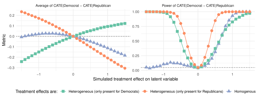
Figure A.6: Note that $N=2883$ partisans. We assess power at the $\alpha=0.05$ level.

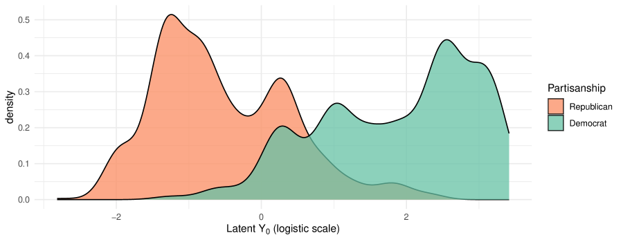
Figure A.7: Distribution of latent $Y_{i}(0)$’s, by party.

References

- (1)
- Abramson, Koçak, and Magazinnik (2022) Abramson, Scott F, Korhan Koçak, and Asya Magazinnik. 2022. “What do we learn about voter preferences from conjoint experiments?” American Journal of Political Science 66 (4): 1008–1020.
- Acharya, Blackwell, and Sen (2016) Acharya, Avidit, Matthew Blackwell, and Maya Sen. 2016. “Explaining causal findings without bias: Detecting and assessing direct effects.” American Political Science Review 110 (3): 512–529.
- Achen and Bartels (2017) Achen, Christopher H., and Larry M. Bartels. 2017. Democracy for Realists: Why Elections Do Not Produce Responsive Government. Princeton, NJ: Princeton University Press.
- Angrist and Pischke (2010) Angrist, Joshua D., and J orn-Steffen Pischke. 2010. “The Credibility Revolution in Empirical Economics: How Better Research Design Is Taking the Con out of Econometrics.” Journal of Economic Perspectives 24 (2): 3–30.
- Ashworth, Berry, and Bueno de Mesquita (2021) Ashworth, Scott, Christopher R Berry, and Ethan Bueno de Mesquita. 2021. Theory and Credibility: Integrating Theoretical and Empirical Social Science. Princeton University Press.
- Ashworth, Berry, and de Mesquita (2023) Ashworth, Scott, Christopher R. Berry, and Ethan Bueno de Mesquita. 2023. “Modeling Theories of Women’s Underrepresentation in Elections.” American Journal of Political Science Early View.
- Ashworth, Bueno de Mesquita, and Friedenberg (2018) Ashworth, Scott, Ethan Bueno de Mesquita, and Amanda Friedenberg. 2018. “Learning about voter rationality.” American Journal of Political Science 62 (1): 37–54.
- Athey, Tibshirani, and Wager (2019) Athey, Susan, Julie Tibshirani, and Stefan Wager. 2019. “Generalized random forests.” Annals of Statistics 47 (2): 1148–1178.
- Athey and Wager (2021) Athey, Susan, and Stefan Wager. 2021. “Policy Learning with Observational Data.” Econometrica 89 (1): 133–161.
- Baccini, Brodeur, and Weymouth (2021) Baccini, Leonardo, Abel Brodeur, and Stephen Weymouth. 2021. “The COVID-19 Pandmeic and the 2020 US Presidential Election.” Journal of Population Economics 34 (2): 739–767.
- Bueno de Mesquita and Tyson (2020) Bueno de Mesquita, Ethan, and Scott A. Tyson. 2020. “The Commensurability Problem: Conceptual Difficulties in Estimating the Effect of Behavior on Behavior.” American Political Science Review 114 (2): 375–391.
- Coppock (2022) Coppock, Alexander. 2022. Persuasion in Parallel. Chicago, IL: University of Chicago Press.
- Devaux and Egami (2022) Devaux, Martin, and Naoki Egami. 2022. “Quantifying Robustness to External Validity Bias.” Working paper available at https://naokiegami.com/paper/external_robust.pdf.
- Dunning (2012) Dunning, Thad. 2012. Natural experiments in the social sciences: a design-based approach. New York: Cambridge University Press.
- Egami and Hartman (2022) Egami, Naoki, and Erin Hartman. 2022. “Elements of external validity: Framework, design, and analysis.” American Political Science Review Forthcoming.
- Fariss, Kenwick, and Reuning (2020) Fariss, Christopher J, Michael R. Kenwick, and Kevin Reuning. 2020. The SAGE Handbook of Research Methods in Political Science and International Relations. Number 20 Thousand Oaks, CA: SAGE Publications chapter Measurement Models, pp. 353–370.
- Fink, McConnell, and Vollmer (2014) Fink, Günther, Margaret McConnell, and Sebastian Vollmer. 2014. “Testing for heterogeneous treatment effects in experimental data: falsediscovery risks and correction procedures.” Journal of Development Effectiveness 6 (1): 44–57.
- Gerber and Green (2012) Gerber, Alan S., and Donald P. Green. 2012. Field Experiments: Design, Analysis, and Interpretation. New York: W.W. Norton.
- Glynn (2012) Glynn, Adam N. 2012. “The product and difference fallacies for indirect effects.” American Journal of Political Science 56 (1): 257–269.
- Grimmer, Messing, and Westwood (2017) Grimmer, Justin, Solomon Messing, and Sean J. Westwood. 2017. “Estimating Heterogeneous Treatment Effects and the Effects of Heterogeneous Treatments with Ensemble Methods.” Political Analysis 25 (4): 413–434.
- Haim, Ravanilla, and Sexton (2021) Haim, Dotan, Nico Ravanilla, and Renard Sexton. 2021. “Sustained Government Engagement Improves Subsequent Pandeic Risk Reporting in Conflict Zones.” American Political Science Review 115 (2): 717–724.
- Healy, Malhotra, and Mo (2010) Healy, Andrew J., Neil Malhotra, and Cecilia Hyunjung Mo. 2010. “Irrelevant events affect voters’ evaluations ofgovernment performance.” Proceedings of the National Academy of Sciences 107 (29): 12804–12809.
- Healy and Malhotra (2010) Healy, Andrew, and Neil Malhotra. 2010. “Random Events, Economic Losses, and Retrospective Voting: Implications for Democratic Competence.” Quarterly Journal of Political Science 5 (2): 193–208.
- Holland (1986) Holland, Paul W. 1986. “Statistics and Causal Inference.” Journal of the American Statistical Association 81 (396): 945–960.
- Imai, Keele, and Tingley (2010) Imai, Kosuke, Luke Keele, and Dustin Tingley. 2010. “A general approach to causal mediation analysis.” Psychological methods 15 (4): 309.
- Imai et al. (2011) Imai, Kosuke, Luke Keele, Dustin Tingley, and Teppei Yamamoto. 2011. “Unpacking the black box of causality: Learning about causal mechanisms from experimental and observational studies.” American Political Science Review 105 (4): 765–789.
- Imai and Yamamoto (2013) Imai, Kosuke, and Teppei Yamamoto. 2013. “Identification and sensitivity analysis for multiple causal mechanisms: Revisiting evidence from framing experiments.” Political Analysis 21 (2): 141–171.
- Kitagawa and Tetenov (2018) Kitagawa, Toru, and Aleksey Tetenov. 2018. “Who Should be Treated? Empirical Welfare Maximization Methods for Treatment Choice.” Econometrica 86 (2): 591–616.
- Kling, Liebman, and Katz (2007) Kling, Jeffrey R., Jeffrey B. Liebman, and Lawrence R. Katz. 2007. “Experimental Analysis of Neighborhood Effects.” Econometrica 75 (1): 83–119.
- Lee and Shaikh (2014) Lee, Soohyung, and Azeem M. Shaikh. 2014. “Multiple Testing and Heterogeneous Treatment Effects: Re-Evaluating the Effect of Progresa on School Enrollment.” Journal of Applied Econometrics 29: 612–626.
- Levy Paluck (2010) Levy Paluck, Elizabeth. 2010. “The Promising Integration of Qualitative Methods and Field Experiments.” The ANNALS of the American Academy of Political and Social Science 628 (1): 59–71.
- Little, Schnakenberg, and Turner (2022) Little, Andrew T., Keith E. Schnakenberg, and Ian R. Turner. 2022. “Motivated Reasoning and Democratic Accountability.” American Political Science Review 116 (2): 751–767.
- Manski (1997) Manski, Charles F. 1997. “Monotone Treatment Response.” Econometrica 65 (6): 1311–1334.
- McClelland and Judd (1993) McClelland, Gary H., and Charles M. Judd. 1993. “Statistical Difficulties of Detecting Interactions and Moderator Effects.” Psychological Bulletin 114 (2): 376–390.
- Moscowitz (2021) Moscowitz, Daniel. 2021. “Local News, Information, and the Nationalization of U.S. Elections.” American Political Science Review 115 (1): 114–129.
- Neyman (1923) Neyman, Jerzy. 1923. “Sur les applications de la theorie des probabilites aux experiences agricoles: essai des principes (Masters Thesis); Justification of applications of the calculus of probabilities to the solutions of certain questions in agricultural experimentation. Excerpts English translation (Reprinted).” Statistical Science 5: 463–472.
- Nilsson et al. (2021) Nilsson, Anton, Carl Bonander, Ulf Strömberg, and Jonas Björk. 2021. “A directed acyclic graph for interactions.” International Journal of Epidemiology 50 (2): 613–619.
- Rubin (1974) Rubin, Donald B. 1974. “Estimating causal effects of treatments in randomized and nonrandomized studies.” Journal of educational Psychology 66 (5): 688.
- Samii (2016) Samii, Cyrus. 2016. “Causal empiricism in quantitative research.” The Journal of Politics 78 (3): 941–955.
- Slough (2022) Slough, Tara. 2022. “Phantom Counterfactuals.” American Journal of Political Science forthcoming.
- Slough and Tyson (2023a) Slough, Tara, and Scott A. Tyson. 2023a. “External Validity and Evidence Accumulation.” Book manuscript.
- Slough and Tyson (2023b) Slough, Tara, and Scott A. Tyson. 2023b. “External Validity and Meta-Analysis.” American Journal of Political Science First View.
- Slough and Tyson (2023c) Slough, Tara, and Scott A. Tyson. 2023c. “Sign-Congruent External Validity and Replication.” Working paper, available at http://taraslough.com/assets/pdf/sc_ev_r.pdf.
- Strezhnev, Kelley, and Simmons (2021) Strezhnev, Anton, Judith G Kelley, and Beth A Simmons. 2021. “Testing for Negative Spillovers: Is Promoting Human Rights Really Part of the “Problem”?” International Organization 75 (1): 71–102.
- Weinberg (2007) Weinberg, Clarice R. 2007. “Can DAGs Clarify Effect Moderation?” Epidemiology 18 (5): 569–572.
- Wolfers (2002) Wolfers, Justin. 2002. “Are Voters Rational? Evidence from Gubernatorial Elections.” Working paper available at https://papers.ssrn.com/sol3/papers.cfm?abstract_id=305740.