Accurate determination of thermoelectric figure of merit using ac Harman method with a four-probe configuration
Abstract
The ac Harman method has been used for the direct estimation of dimensionless thermoelectric figure of merit () through ac/dc resistance measurements. However, accurate estimation with a four-probe configuration is difficult owing to the occurrence of a thermal phase-delay in the heat flow with a low frequency current. This study reports an exact solution for estimation by solving the heat conduction equation. The analysis can explain the reverse heat flow, which is the main source of the error in the four-probe configuration, and the experimentally obtained behavior of the frequency dependence of of (Bi,Sb)2Te3. Approximately of the error is caused by a thermal phase-delay, unless an appropriate current frequency and voltage-terminal position are chosen. Thus, an accurate evaluation using a four-probe configuration at any voltage terminal position is achieved. These findings can lead to interesting thermoelectric metrology and could serve as a powerful tool to search for promising thermoelectric materials.
I Introduction
Thermoelectric (TE) materials are expected to contribute to power generation in situ as they facilitate the efficient conversion of waste heat into electrical energy Bell (2008); Zhang and Zhao (2015); He and Tritt (2017). The conversion efficiency of TE materials depends on the dimensionless figure of merit , which is defined as , where , , , and denote the Seebeck coefficient, absolute temperature, electrical resistivity, and thermal conductivity, respectively Rowe (1995). The accurate evaluation of the of TE materials requires independent measurements of the three physical parameters (, , and ). Generally, such measurements are performed by employing different experimental setups and sample shapes, which can affect the accuracy of estimation. In a recent international round-robin test, the interlaboratory uncertainty for was estimated to be approximately to Wang et al. (2013, 2015); Alleno et al. (2015); Heremans and Martin (2024). Consequently, the establishment of standardized and accurate measurement techniques to realize the precise estimation of TE properties is desirable.
The ac Harman method is an alternative method to determine . It enables the direct determination of through ac and dc resistance measurements using the following formula
| (1) |
where and denote the resistances of the sample measured via application of dc and ac currents, respectively Harman (1958). The ac Harman method exploits the Peltier effect, which occurs at the sample edges upon the application of the current to the sample. The ac Harman method has been extensively used for a simple estimation procedure in the case of various targets, such as minute crystals, thin films, and module composite structures, because it can be performed based on a simple two-probe configuration Satake et al. (2004); Kobayashi et al. (2008, 2009); Singh et al. (2009); Venkatasubramanlan et al. (2001); Iwasaki et al. (2003); Korzhuev et al. (2011); Barako et al. (2012); Muto et al. (2009).
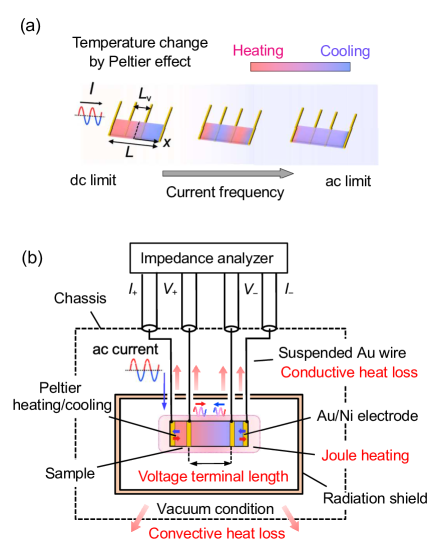
To accurately perform resistance measurements, it is generally more effective to use a four-probe configuration rather than the two-probe configuration. The advantage of the four-probe configuration is that it can discard the influence of wiring (contact) resistance. However, important error factors that are unique to a four-probe configuration exist, which are caused by an inhomogeneous temperature gradient in a particular low-frequency region (Fig. 1(a)). The experimentally estimated using a four-probe configuration varies significantly as a function of the distances between the two voltage-terminals Iwasaki et al. (2004). Although this error factor is known phenomenologically as a thermal phase delay when using the ac Harman method with the four-probe configuration Iwasaki and Hori (2015); Downey et al. (2007), analytical and experimental validation are lacking.
This study reports a general expression for the ac Harman method with a four-probe configuration. The exact solution of the temperature distribution in the sample was derived from the heat conduction equation that incorporates the Joule effect. Moreover, experiments were performed to estimate using Bi-Te materials, and the results are consistent with the exact solution over a wide frequency range. Thus, the proposed analysis facilitates an accurate estimation using the ac Harman method with a four-probe configuration at an arbitrary voltage terminal distance.
II Theory
II.1 Exact solution of temperature distribution in a material
Figure 1(b) shows a schematic of the setup of the ac Harman method with a four-probe configuration. Herein, the case where resistance measurement is performed on a rectangular parallelepipedal sample with a sample length and cross-sectional area using the four-probe configuration at a voltage terminal distance is considered. The temperature distribution in the sample (,) when an ac current with a current density can be obtained by solving the following one-dimensional unsteady heat conduction equation,
| (2) |
where, , , , , and represent the position, time, peak current density, current angular velocity, and thermal diffusivity, respectively. The second term on the right-hand side represents the Joule effect. The Joule heat was considered to incorporate the current amplitude dependence. It was assumed that the values of the physical properties were independent of the temperature. To simplify the boundary condition, it was assumed that only the Peltier heat occurred at both ends of the sample , where denotes the average temperature of the sample. Consequently, the boundary condition is described as
| (3) |
Under this boundary condition, is expressed as follows:
| (4) |
| (8) |
where, and denote the reciprocal of thermal diffusion length and an imaginary number. and are defined as contribution of the Peltier and Joule effects.
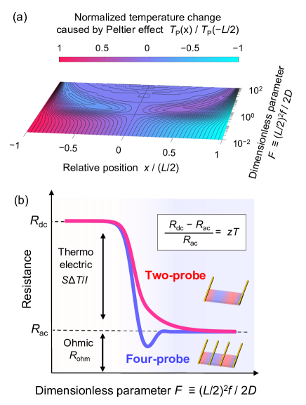
A characteristic dimensionless parameter, , was introduced to represent the thermal response of the sample, which can classify the behavior of the temperature distribution Okawa et al. (2021). Figure 2(a) shows a contour plot of the temperature change in the - plane when the root-mean-square (rms) ac current is applied. The solid lines represent isothermal lines. The temperature changes were normalized to one of the sample edges . Evidently, a temperature difference in the opposite direction in the sample occurred when . The direction of the was periodically inverted as the polarity of the current was reversed. Such a non-uniform represents a thermal phase delay with respect to the current, which corresponds to insufficient cancellation of the TE effect because the phase of the thermal wave could not match the thermal response of the sample. Thus, measurements using the four-probe configuration in this region have a significant effect on the measured resistance and is among the main primary sources of error in the evaluation, as shown in Fig. 2(b). An ac current of a sufficiently high frequency can cancel the TE effect (i.e., ) to yield, a flat for the sample end. Consequently, sufficiently accurate measurements can be performed by connecting the voltage terminals at this flat temperature position.
II.2 Exact solution of the resistance for estimation
Subsequently, using the obtained (,), the measured resistance can be expressed as follows, with ohmic resistance and resistance contributed from the Joule effect :
| (9) |
where and are expressed as the following functions:
| (10) |
where and are defined as functions that are dependent on and , respectively. To perform the evaluation, Eq. (1) can be rewritten as follows:
| (11) |
Equation (11) is a general expression for estimation using the ac Harman method with a four-probe configuration, considering the Joule effect in the time domain. It can appropriately explain the frequency characteristics of measured with four-probe configuration. See Appendix for further calculation details. In Eq. (11), depends on the TE properties of the samples () and the characteristic parameters ( and ). If the thermal diffusivity , sample length , and voltage terminal distance are known in advance, the characteristic parameters , and can be determined. Generally, for accurate estimation, the current frequency should be chosen such that the dimensionless parameter , as shown in Fig. 2. In our model, can be estimated at any voltage terminal distance using Eq. (8). Furthermore, if the dependence of can be measured, Eq. (8) can be used to estimate the thermoelectric parameters ( and ) through fitting. The thermoelectric parameters ( and ) are the fitting parameters. The electrical resistivity is estimated using the measured and sample length .
III Experimental setup
Experiments were performed using bulk samples to validate the proposed analytical model. The measurements were performed using a sintered polycrystalline sample of p-type Bi0.3Sb1.7Te3 (Toshima Manufacturing Co., Ltd.)Okawa et al. (2020). The Bi–Te and Sb–Te powders were sintered using the hot isostatic press (HIP) method to obtain ingots. The dimensions of the samples are . Au/Ni electrodes were fabricated via sputtering to sufficiently secure the Peltier heat generated at the edge of the sample. The heat loss from conduction through the wiring was suppressed by reducing the thickness of the Au wires, which adhered to the sample with Ag paste. To suppress the influence of the heat convection, the apparatus was assembled in a vacuum chamber, and measurements were performed at a high vacuum of or less. The sample was suspended using the thin Au wires of sufficient length to improve its thermal isolation conditions. Additionally, the sample space was covered with a radiation shield to reduce heat loss owing to thermal radiation. To realize quantitative correction of the radiation effects, measurements can be performed at higher temperatures and corrected for the measurements of other TE properties Ao et al. (2011). The ac and dc resistances of the samples were measured using an impedance analyzer. A coaxial cable was used to connect the case, and measurements were performed using a four-probe configuration.
IV Results and discussion
IV.1 Current-frequency dependence of the resistance
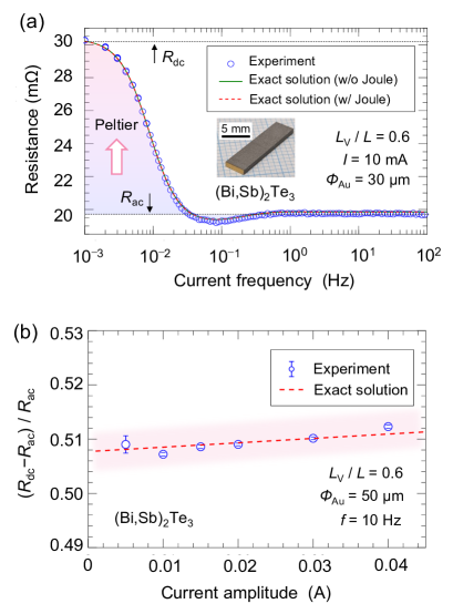
We demonstrate the correctness of the exact solution and evaluation using a four-probe configuration. Figure 3(a) shows the experimental and calculated results of the current-frequency dependence of the resistance for (Bi,Sb)2Te3. The open symbols represent the experimental results for and a wire diameter of . The normalized distance between the voltage terminals is 0.6. The calculation used the typical physical properties of (Bi,Sb)2Te3 at room temperature . At current frequencies less than , the measured resistance approaches , and the TE effect was sufficiently generated. However, it gradually decreased to as the current frequency increased. Moreover, a dip structure occurs at , corresponding to in Fig. 2. It is caused by a phase shift owing to the thermal wave and thermal response of the sample. The voltage is detected at the points where the temperature change is opposite direction to the temperature difference between the two ends of the sample . This is referred to as the “thermoinductive effect”Okawa et al. (2021). As described later, this resulted in the overestimation of , which is evident from the dependence of . Such a dip structure is not observed in the two-probe configuration when ; however, it is underestimated compared to unless a sufficiently high frequency is chosen (Fig. 2(b)). This is consistent with the lack of a dip structure in two-probe measurements Shinozaki et al. (2020); Hasegawa and Takeuchi (2022, 2023); Marchi and Giaretto (2011); Marchi et al. (2013); Apertet and Ouerdane (2017); Beltran-Pitarch and Prado-Gonjal (2018); Beltran-Pitarch et al. (2020a); Arisaka et al. (2019); Beltran-Pitarch et al. (2020b); Yoo et al. (2019); Otsuka et al. (2020); Zaoui et al. (2020); Hasegawa and Takeuchi (2021); Beltran-Pitarch et al. (2021); Hirabayashi and Hasegawa (2021); Korzhuev and Avilov (2010). Thus, the ac Harman method can be used to determine over a wide frequency range of the four-probe configuration using the exact solution derived.
IV.2 Influence of the Joule effect
Subsequently, the influence of the Joule effect was investigated. The red and green lines shown in Fig. 3(a) represent the calculation results based on the exact solution with and without considering the Joule effect, respectively. As Joule heating is time-dependent, the measured resistance was calculated over the time of one measurement cycle at each frequency. When , the influence of the Joule effect was not observed at most frequencies. Figure 3(b) illustrates the relationship between and the current amplitude. The experimental results are shown for current values in the range of to with , , and = 0.6. The error bars represent the standard deviation of the mean obtained from independent measurements. increases linearly with the current amplitude. The result is consistent with the calculation line based on the exact solution.
At , was estimated to be 0.509, which increased to 0.511 at . If the higher order TE effect, the Thomson heat induced by the Joule effect, would be proportional to the square of the current at high current region. Upon applying a large current of or more, the sample and wiring heat up, which renders accurate evaluation and correction difficult. The optimal current amplitude can be determined by comparing the Peltier heat generated in the measurement system with the Joule heat and then choosing a suitable compromise between the degree of measurement noise generated by the setup and Joule heat Hasegawa and Takeuchi (2021).
IV.3 Suitable measurement conditions for the ac Harman method with four-probe configuration
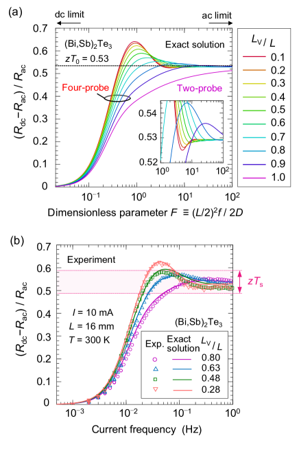
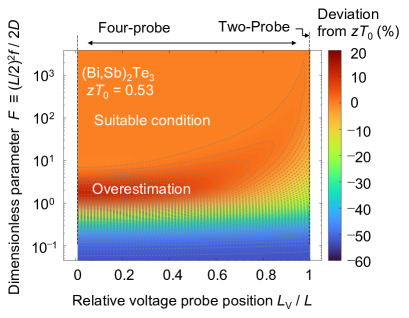
Figure 4 presents the experimental and calculated results based on the exact solution of for different values. Figure 4(a) shows the dependence of on the exact solution of , where a smaller and larger could be considered as dc and ac limits, respectively. was varied from 0.1 to 1.0. For an value of approximately 1, the smaller the , the larger the dip structure. It can be attributed to the thermal phase delay (as a thermoinductive effect) and is a measurement error that only occurs in the four-probe configuration, as described above. The intrinsic value of dimensionless figure of merit can be determined using at the ac limit. The value of changes significantly with respect to , and it is evident that the maximum deviation is . It was quantitatively shown that the choice of the current frequency causes an error in evaluation for the ac Harman method.
Figure 4(b) illustrates the experimental results of the frequency dependence of . was varied from 0.28 to 0.80. For the value of 0.28, a large dip structure was observed at approximately . For all results, consistency was obtained with the exact solution over a wide frequency range. As the dimensionless resistance in Eq. (11) depends on , the current frequency to be selected differs based on sample length and thermal diffusivity . Therefore, it is not always necessary to select an appropriate current frequency when measuring samples of different sizes and compositions. However, for an ac bridge used for accurate resistance measurement, the selection of the measurement frequency must be focused upon. When measuring higher frequencies, the influence of the parasitic effects, inherent to the high frequency, depends on the circuit; therefore, the frequency must be checked for each instance. As depicted in Fig. 5, the suitable experimental condition for the ac Harman method was identified visually.
To verify the estimated value, independent measurements of the Seebeck coefficient, electrical resistivity, and thermal conductivity were performed at 300 K. The rectangular bars cut from the ingots were used to measure the electrical resistivity () and the Seebeck coefficient () using ZEM-3 (ULVAC Co., Ltd.). The power factor, defined as , was calculated (). The materials demonstrate a relatively high power-factor of approximately at . The thermal conductivity () of the materials was determined using the formula , in which is the thermal diffusivity, represents the density, and denotes the specific heat of the materials. The thermal diffusivity was measured via a laser flash method , and the density was measured using the Archimedes method . The specific heat of the material was determined to be based on the literature values for Bi2Te3 () and Sb2Te3 () Chen (2011). The thermal conductivity was calculated using the measured , , and the estimated . The dimensionless figure of merit was calculated using the standard formula and is 0.538. In a report on the international round-robin test using bulk bismuth telluride, the scatter for was estimated to be approximately at 300 K Wang et al. (2013). The typical error in estimating from resistance measurement using the Harman formula is reported to be about d. Boor and Schmidt (2010). The evaluation results using the standard formula are in agreement with those obtained using the ac Harman method, as shown in Fig. 4(b).
IV.4 Examination of accuracy and influence of other error factors
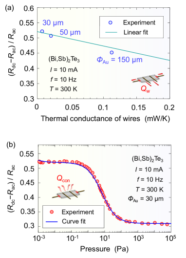
Thus far, we presented error factors such as the current frequency , current amplitude , and voltage terminal distance , which have not been quantitatively identified using exact solutions. Subsequently, we discuss the other significant error factors, excluding dimensionless parameter , , and the Joule effect. The ac Harman method assumes that all Peltier heat generated at the sample edge flows into the sample. In an actual experimental environment, various heat losses occur, such as conduction through the lead wire , and heat convection , which results in a crucial error factor in the estimation Kwon et al. (2014); Penn (1964); Campbell et al. (1965); Iwasaki et al. (2002); Kang et al. (2016); Roh et al. (2016); Putilin and Yuragov (2003); Mccarty et al. (2012); Vasilevskiy et al. (2014). The exact solutions comprehensively consider and combined with other TE effects; however, it is extremely difficult to introduce using the unsteady heat conduction equation. Our results of the resistance measurements for different wire diameters with , and are shown in Fig. 6(a). Considering an energy balanceKwon et al. (2014), the ratio of the thermal conductance of the lead wire to that of the sample determines . The results of the resistance measurements with wire diameter in the range of to exhibits that is underestimated as increases. The result is quantitatively consistent with the relationship expressed as derived by a linear fitting. Thus, reduction in can alleviate the underestimation of owing to the . A wire with a smaller diameter has the effect of lowering the upper limit of the maximum applied current, which is a trade-off in an actual experimental environment.

As shown in Fig. 6(b), resistance measurements were performed by varying the pressure in the sample chamber from ambient pressure to with , , and . At ambient pressure, can be underestimated by up to compared with that in a high vacuum. A sharp decrease in was observed from to . This can be attributed to the transition from the viscous to the molecular flow regime, resulting in an increase in the number of molecules responsible for heat conduction, leading to increased convective heat loss . Analytically, the introduction of the heat transfer term within the heat conduction equation yields the relationship , where and are the heat-transfer coefficient and perimeter of the sample, respectively. Fitting with this relationship yielded results that are consistent with the experimental results over a wide range of pressures. For our setup, the influence of can be neglected in a vacuum environment above .
The existence of inhomogeneous Peltier heating at the edge of the sample/electrode junctions also causes a underestimation for Beltran-Pitarch et al. (2019). In our setup, the effect of inhomogeneous current application was avoided through the formation of Ni/Au electrodes at both ends of the (Bi,Sb)2Te3. Furthermore, the heat radiation leads to significant underestimation up to at high temperatures, Ao et al. (2011). With proper installation of radiation shielding, the influence of the radiation heat loss can be reduced at room temperature.
The primary error factors were identified as described above. The insights gained in this analysis enable accurate estimation measured using four-probe configuration measurements. Notably, some known physical parameters are required to fully compensate for error factors, which is also true for other evaluation methods. For example, in the two-probe based impedance measurement, which is an accurate measurement technique with a similar concept, the frequency dependence of impedance is measured in advance over a wide range Shinozaki et al. (2020); Hasegawa and Takeuchi (2022, 2023); Marchi and Giaretto (2011); Marchi et al. (2013); Apertet and Ouerdane (2017); Beltran-Pitarch and Prado-Gonjal (2018); Beltran-Pitarch et al. (2020a); Arisaka et al. (2019); Beltran-Pitarch et al. (2020b); Yoo et al. (2019); Otsuka et al. (2020); Zaoui et al. (2020); Hasegawa and Takeuchi (2021); Beltran-Pitarch et al. (2021); Hirabayashi and Hasegawa (2021); Korzhuev and Avilov (2010). Consequently, several thermophysical properties can be estimated using analytical models in the frequency domain. Since the TE module system tends to be relatively complex within the time domain, the analysis is used within the frequency domain Zaoui et al. (2020). In the two-probe configuration, the contact resistance between the sample and electrode must be considered, which necessitates its analysis. Furthermore, the influence of contact resistance is inevitable. Experimental studies, such as preparing a sample shape, wherein this influence can be ignored, are necessary Beltran-Pitarch et al. (2019). For accurate resistance measurement, the use of a four-probe configuration that requires knowledge of the voltage terminal distance is beneficial. Note that the error in the evaluation of the voltage terminal distance and the thermal diffusivity has an influence on our analysis. The measurement of the voltage terminal distance is more influenced by shorter sample lengths or larger wire diameters. It has been suggested that the error of length measurement tend to be quite large () in small samples Heremans and Martin (2024).
IV.5 estimation of other sample
To demonstrate the universality of our technique, we have also applied the ac Harman method to estimate the of n-type Bi2Te3 (Toshima Manufacturing Co., Ltd.) using the same sample geometry as the p-type Bi0.3Sb1.7Te3. Figure 7 shows the frequency dependence of the resistance and of n-type Bi2Te3 with and . The normalized distance between the voltage terminals is 0.3. Notable dip structures were observed around 50 mHz in the frequency dependences of the resistance and . This frequency region roughly corresponds to . The plots developed using the exact solution, agreed well with the experimental results over a wide frequency range. The value of dimensionless figure of merit can be determined using the measurement data. The physical properties of n-type Bi2Te3 (, , and ) at were used in the calculation. As with the case of p-type Bi0.3Sb1.7Te3, the Seebeck coefficient and electrical resistivity were measured using ZEM-3 and found to be and , respectively. The dimensionless figure of merit using the standard formula is calculated 0.39, in which the thermal conductivity is assumed the same value as the p-type Bi0.3Sb1.7Te3 (). The evaluation results using the standard formula are in agreement with those obtained using the ac Harman method. The present analysis is applicable to other thermoelectric materials.
V Conclusion
In this study, the evaluation equation of the ac Harman method was derived for a four-probe configuration from the exact solution, which was then experimentally verified. The effects of the distance between the voltage terminals, current frequency, Joule effect, and convective heat transfer, which have been empirically avoided, were clarified. Using the evaluation formula, each error factor was avoided or corrected. The analysis performed provided information on evaluation errors caused by the position of the voltage terminal attachments, as well as heat losses owing to thermal convection, heat conduction of the lead wires, and the Joule effect. As described above, this study realized the correction of various heat losses that are inevitable when measuring using the ac Harman method, and a more accurate determination of can be realized through further systematic empirical research.
Acknowledgements
This work was supported by a Grant-in-Aid for Research Activity Start-up (Grant No.17H07399) from the Japan Society for Promotion of Science (JSPS), Grant-in-Aid for Early-Career Scientists (Grant No.23K13552) from JSPS, the Thermal & Electric Energy Technology Foundation (TEET), Iketani Science and Technology Foundation, and the Precise Measurement Technology Promotion Foundation (PMTP-F).
Appendix: Calculation details for exact solution of estimation
The temperature distribution in the sample at position and time is expressed as Eq. (4) and Eq. (5). The contribution from the Peltier effects can be obtained by solving the following one-dimensional unsteady-state heat transfer equation Okawa et al. (2021); Kirby and Laubitz (1973):
| (12) |
According to the method of separation of variables, the general solution of Eq. (9) is described as
| (13) |
where and are arbitrary constants. is the reciprocal of thermal diffusion length . Under the boundary condition Eq. (3), and are obtained.
| (14) |
| (15) |
is given by Eq. (5). The contribution from the Joule effects can be obtained by solving the following equation under the boundary condition Dunn et al. (2019); Dames and Chen (2005); Lu et al. (2001):
| (16) |
Using obtained from Eq. (5), the voltage measured between is expressed as follows:
| (17) | |||||
The first term on the right side represents the ohmic voltage between , and the second term represents the Seebeck voltage. In actual measurements, the temperature rise caused by the Peltier and Joule effects at low current region is considered small , so the integral part can be replaced with . The measured resistance in Eq. (6) can be introduced as :
| (18) | |||||
The equation can be rewritten using and :
| (19) |
where
| (20) | ||||
| (21) |
Using Eq. (7), the resistance can be expressed as Eq. (6). In the dc limit, the current frequency , and is expressed as:
| (22) |
The resistances of the sample measured via application of dc and ac currents, and are obtained as:
| (23) | |||||
| (24) |
To perform the evaluation, Eq. (1) can be rewritten as follows:
| (25) | |||||
References
- Bell (2008) L. E. Bell, Science 321, 1457 (2008).
- Zhang and Zhao (2015) X. Zhang and L.-D. Zhao, J. Materiomics 1, 92 (2015).
- He and Tritt (2017) J. He and T. M. Tritt, Science 357, 1369 (2017).
- Rowe (1995) D. M. Rowe, CRC Press 18, 189 (1995).
- Wang et al. (2013) H. Wang, W. D. Porter, H. Böttner, J. König, L. Chen, S. Bai, T. M. Tritt, A. Mayolet, J. Senawiratne, C. Smith, F. Harris, P. Girbert, J. W. Sharp, J. Lo, H. Kleinke, and L. Kiss, J. Electron. Mater. 42, 654 (2013).
- Wang et al. (2015) H. Wang, S. Bai, L. Chen, A. Cuenat, G. Joshi, H. Kleinke, J. König, H. W. Lee, J. Martin, M.-W. Oh, W. D. Porter, Z. Ren, J. Salvador, J. Sharp, P. Taylor, A. J. Thompson, and Y. C. Tseng, J. Electron. Mater. 44, 4482 (2015).
- Alleno et al. (2015) E. Alleno, D. Bérardan, C. Byl, C. Candolfi, R. Daou, R. Decourt, E. Guilmeau, S. Hébert, J. Hejtmanek, B. Lenoir, P. Masschelein, V. Ohorodnichuk, M. Pollet, S. Populoh, D. Ravot, O. Rouleau, and M. Soulier, Rev. Sci. Instrum. 86, 011301 (2015).
- Heremans and Martin (2024) J. P. Heremans and J. Martin, Nature Materials 23, 18 (2024).
- Harman (1958) T. C. Harman, J. Appl. Phys. 29, 1373 (1958).
- Satake et al. (2004) A. Satake, H. Tanaka, T. Ohkawa, T. Fujii, and I. Terasaki, J. Appl. Phys. 96, 931 (2004).
- Kobayashi et al. (2008) W. Kobayashi, W. Tamura, and I. Terasaki, J. Phys. Soc. Jpn. 77, 07606 (2008).
- Kobayashi et al. (2009) W. Kobayashi, W. Tamura, and I. Terasaki, J. Electron. Mater. 38, 964 (2009).
- Singh et al. (2009) R. Singh, Z. Bian, A. Shakouri, G. Zeng, J.-H. Bahk, J. E. Bowers, J. M. O. Zide, and A. C. Gossard, Appl. Phys. Lett. 94, 212508 (2009).
- Venkatasubramanlan et al. (2001) R. Venkatasubramanlan, E. Silvola, T. Colpitts, and B. O’Quinn, Nature 413, 597 (2001).
- Iwasaki et al. (2003) H. Iwasaki, S. Yokoyama, T. Tsukui, M. Koyano, H. Hori, and S. Sano, Jpn. J. Appl. Phys. 42, 3703 (2003).
- Korzhuev et al. (2011) M. A. Korzhuev, E. S. Avilov, and I. Y. Nichezina, J. Electron. Mater. 40, 733 (2011).
- Barako et al. (2012) M. Barako, W. Park, A. Marconnet, M.Asheghi, and K. Goodson, J. Electron. Mater. 42, 372 (2012).
- Muto et al. (2009) A. Muto, D. Kraemer, Q. Hao, Z. F. Ren, and G. Chen, Rev. Sci. Instrum. 80, 093901 (2009).
- Iwasaki et al. (2004) H. Iwasaki, M. Koyano, Y. Yamamura, and H. Hori, Solid State Commun. 130, 507 (2004).
- Iwasaki and Hori (2015) H. Iwasaki and H. Hori, in International Conference on Thermoelectrics, ICT Proceedings , 501 (2015).
- Downey et al. (2007) A. D. Downey, T. P. Hogan, and B. Cook, Rev. Sci. Instrum. 78, 093904 (2007).
- Okawa et al. (2021) K. Okawa, Y. Amagai, H. Fujiki, and N.-H. Kaneko, Commun. Phys. 4, 267 (2021).
- Okawa et al. (2020) K. Okawa, Y. Amagai, H. Fujiki, N.-H. Kaneko, N. Tsuchimine, H. Kaneko, Y. Tasaki, K. Ohata, M. Okajima, and S. Nambu, Japanese Journal of Applied Physics 59, 046504 (2020).
- Ao et al. (2011) X. Ao, J. de Boor, and V. Schmidt, Adv. Energy Mater. 1, 1007 (2011).
- Shinozaki et al. (2020) R. Shinozaki, S. Hirabayashi, and Y. Hasegawa, Appl. Phys. Express 13, 106501 (2020).
- Hasegawa and Takeuchi (2022) Y. Hasegawa and M. Takeuchi, Sci. Rep. 12, 11967 (2022).
- Hasegawa and Takeuchi (2023) Y. Hasegawa and M. Takeuchi, Rev. Sci. Instrum. 94, 014902 (2023).
- Marchi and Giaretto (2011) A. D. Marchi and V. Giaretto, Rev. Sci. Instrum. 82, 034901 (2011).
- Marchi et al. (2013) A. D. Marchi, V. Giaretto, S. Caron, and A. Tona, J. Electron. Mater. 42, 2067 (2013).
- Apertet and Ouerdane (2017) Y. Apertet and H. Ouerdane, Energy Conversion and Management 149, 564 (2017).
- Beltran-Pitarch and Prado-Gonjal (2018) B. Beltran-Pitarch and J. Prado-Gonjal, J. Appl. Phys. 123, 084505 (2018).
- Beltran-Pitarch et al. (2020a) B. Beltran-Pitarch, J. Prado-Gonjal, A. V. Powell, P. Ziolkowski, and J. Garcia-Canadas, J. Appl. Phys. 165, 114361 (2020a).
- Arisaka et al. (2019) T. Arisaka, M. Otsuka, and Y. Hasegawa, Rev. Sci. Instrum. 90, 046104 (2019).
- Beltran-Pitarch et al. (2020b) B. Beltran-Pitarch, F. Vidan, and J. Garcia-Canadas, Appl. Thermal Engineering 165, 114361 (2020b).
- Yoo et al. (2019) C.-Y. Yoo, C. Yeon, Y. Jin, Y. Kim, J. Song, H. Yoon, S.-H. Park, B. Beltran-Pitarch, J. Prado-Gonjal, and G. Min, Appl. Energy 251, 113341 (2019).
- Otsuka et al. (2020) M. Otsuka, T. Arisaka, and Y. Hasegawa, Materials Science & Engineering B 261, 114620 (2020).
- Zaoui et al. (2020) S. Zaoui, A. Belayadi, M.Zabat, A. Mougari, and F. Mekideche-Chafa, Physica B 580, 411735 (2020).
- Hasegawa and Takeuchi (2021) Y. Hasegawa and M. Takeuchi, Rev. Sci. Instrum. 92, 083902 (2021).
- Beltran-Pitarch et al. (2021) B. Beltran-Pitarch, J. Maassen, and J. Garcia-Canadas, Appl. Energy 299, 117287 (2021).
- Hirabayashi and Hasegawa (2021) S. Hirabayashi and Y. Hasegawa, Jpn. J. Appl. Phys. 60, 106503 (2021).
- Korzhuev and Avilov (2010) M. A. Korzhuev and E. S. Avilov, J. Electron. Mater. 39, 1499 (2010).
- Chen (2011) X. Chen, Appl. Phys. Lett. 99, 261912 (2011).
- d. Boor and Schmidt (2010) J. d. Boor and V. Schmidt, Adv. Mater. 22, 4303 (2010).
- Kwon et al. (2014) B. Kwon, S.-H. Baek, S. K. Kim, and J.-S. Kim, Rev. Sci. Instrum. 85, 045108 (2014).
- Penn (1964) A. W. Penn, J. Sci. Instrum 41, 626 (1964).
- Campbell et al. (1965) M. R. Campbell, C. A. Hogarth, and C. A. Hagger, Int. J. Electron. 19, 571 (1965).
- Iwasaki et al. (2002) H. Iwasaki, M. Koyano, and H.Hori, Jpn. J. Appl. Phys. 41, 6606 (2002).
- Kang et al. (2016) M.-S. Kang, I.-J. Roh, Y. G. Lee, S.-H. Baek, S. K. Kim, B.-K. Ju, D.-B. Hyun, J.-S. Kim, and B. Kwon, Sci. Rep. 6, 26507 (2016).
- Roh et al. (2016) I.-J. Roh, Y. G. Lee, M.-S. Kang, J.-U. Lee, S.-H. Baek, S. K. Kim, B.-K. Ju, D.-B. Hyun, J.-S. Kim, and B. Kwon, Sci. Rep. 6, 39131 (2016).
- Putilin and Yuragov (2003) A. B. Putilin and E. A. Yuragov, Measurement Techniques 46, 1173 (2003).
- Mccarty et al. (2012) R. Mccarty, J. Thompson, J. Sharp, A. Thompson, and J. Bierschenk, J. Electron. Mater. 41, 1274 (2012).
- Vasilevskiy et al. (2014) D. Vasilevskiy, J.-M. Simard, R. A. Masut, and S. Turenne, J. Electron. Mater. 44, 1733 (2014).
- Beltran-Pitarch et al. (2019) B. Beltran-Pitarch, J. Prado-Gonjal, A. V. Powell, and J. Garcia-Canadas, J. Appl. Phys. 125, 025111 (2019).
- Kirby and Laubitz (1973) C. G. Kirby and M. J. Laubitz, Metrologia 9, 103 (1973).
- Dunn et al. (2019) I. H. Dunn, R. Daou, and C. Atkinson, Rev.Sci. Instrum. 90, 024902 (2019).
- Dames and Chen (2005) C. Dames and G. Chen, Rev. Sci. Instrum. 76, 124902 (2005).
- Lu et al. (2001) L. Lu, W. Yi, and D. L. Zhang, Rev. Sci. Instrum. 72, 2996 (2001).