Nonfactorizable charming-loop contribution to FCNC $B_{s}\to\gamma l^{+}l^{-}$ decay

Abstract

We present the first theoretical calculation of nonfactorizable charm-quark loop contributions to the $B_{s}\to\gamma l^{+}l^{-}$ amplitude. We calculate the relevant form factors, $H_{A,V}^{\rm NF}(k^{\prime 2},k^{2})$, and provide convenient parametrizations of our results in the form of fit functions of two variables, $k^{\prime 2}$ and $k^{2}$, applicable in the region below hadron resonances, $k^{\prime 2}<M_{J/\psi}^{2}$ and $k^{2}<M_{\phi}^{2}$. We report that factorizable and nonfactorizable charm contributions to the $B_{s}\to\gamma l^{+}l^{-}$ amplitude have opposite signs. To compare the charm and the top contributions, it is convenient to express the NF charming loop contribution as a non-universal (i.e., dependent on the reaction) $q^{2}$-dependent correction $\Delta^{\rm NF}C_{7}(q^{2})$ to the Wilson coefficient $C_{7}$. For the $B_{s}\to\gamma l^{+}l^{-}$ amplitude, the correction is found to be positive, $\Delta^{\rm NF}C_{7}(q^{2})/C_{7}>0$.

I Introduction

This paper reports the first theoretical analysis of nonfactorizable (NF) charming loops in rare flavour-changing neutral currents (FCNC) $B_{s}\to\gamma l^{+}l^{-}$ decays making use of theoretical approach formulated in bbm2023 .

Charming loops in rare FCNC decays of the $B$-meson have visible impact on the $B$-decay observables neubert and their reliable theoretical description is necessary for studies of possible new physics effects (see, e.g., ciuchini2022 ; ciuchini2020 ; ciuchini2021 ; diego2021 ; matias2022 ; gubernari2022 ; hurth2022 ; stangl2022 ; diego2023a ; diego2023b ).

A number of theoretical analyses of nonfactorizable (NF) charming loops in FCNC $B$-decays has been published in the recent years: In voloshin , an effective gluon-photon local operator describing the charm-quark loop has been calculated as an expansion in inverse charm-quark mass $m_{c}$ and applied to inclusive $B\to X_{s}\gamma$ decays (see also ligeti ; buchalla ); in khod1997 , NF corrections in $B\to K^{*}\gamma$ using local operator product expansion (OPE) have been studied; NF corrections induced by a local photon-gluon operator have been calculated in zwicky1 ; zwicky2 in terms of the light-cone (LC) 3-particle antiquark-quark-gluon Bethe-Salpeter amplitude (3BS) of $K^{*}$-meson braun ; ball1 ; ball2 with two field operators having equal coordinates, $\langle 0|\bar{s}(0)G_{\mu\nu}(0)u(x)|K^{*}(p)\rangle$, $x^{2}=0$. As noticed already long ago, local OPE for the charm-quark loop in FCNC $B$-decays leads to a power series in $\Lambda_{\rm QCD}m_{b}/m_{c}^{2}\simeq 1$. To sum up numerically large $O(\Lambda_{\rm QCD}m_{b}/m_{c}^{2})^{n}$ corrections, Ref. hidr obtained a nonlocal photon-gluon operator describing the charm-quark loop and evaluated its effect making use of 3BS of the $B$-meson in a collinear LC configuration $\langle 0|\bar{s}(x)G_{\mu\nu}(ux)b(0)|\bar{B}_{s}(p)\rangle$, $x^{2}=0$ japan ; braun2017 . The same collinear approximation [known to provide the dominant 3BS contribution to meson tree-level form factors braun1994 ; offen2007 ] was applied also to the analysis of other FCNC $B$-decays gubernari2020 .

In later publications mk2018 ; m2019 ; m2022 ; m2023 , it was proven that the dominant contribution to FCNC $B$-decay amplitudes is actually given by the convolution of a hard kernel with the 3BS in a different configuration — a double-collinear light-cone configuration $\langle 0|\bar{s}(y)G_{\mu\nu}(x)b(0)|\bar{B}_{s}(p)\rangle$, where $y^{2}=0$, $x^{2}=0$, but $x\,y\neq 0$. The corresponding factorization formula was derived in m2023 . The first application of a double-collinear 3BS to FCNC $B_{s}\to\gamma\gamma$ decays was presented in wang2022 ; wang2023 .

As a further step, bbm2023 developed a theoretical approach to NF charming loops in FCNC $B$-decays based on a generic 3BS of the $B$-meson. This approach makes use of rigorous properties of the generic 3BS: Namely, the generic 3BS of the $B$-meson contains new Lorentz structures (compared to the collinear and the double-collinear configurations) and new three-particle distribution amplitudes (3DAs) that appear as the coefficients multiplying these Lorentz structures; analyticity and continuity of the 3BS as the function of its arguments at the point $xp=yp=x^{2}=y^{2}=0$ leads to certain constraints on the 3DAs m2023 which were implemented in the 3BS model of bbm2023 . Moreover, bbm2023 applied this approach to $B_{s}\to\gamma\gamma$ decays.

Here we extend the analysis of bbm2023 to the case of $B_{s}\to\gamma l^{+}l^{-}$ decays. The paper is organized as follows: Sect. II recalls general formulas for the top contribution to the $B_{s}\to\gamma l^{+}l^{-}$ amplitude and describes the connection between the charm contribution to the amplitudes of $B_{s}\to\gamma l^{+}l^{-}$ and $B_{s}\to\gamma^{*}\gamma^{*}$ containing two virtual photons in the final state, including constraints on the latter imposed by electromagnetic gauge invariance. Section III outlines the calculation of the factorizable and nonfactorizable charming-loop contributions to the $B_{s}\to\gamma^{*}\gamma^{*}$ amplitude. Section IV gives numerical predictions for the form factors $H_{A,V}^{\rm NF}(k^{\prime 2},k^{2})$ describing NF charm in $B_{s}\to\gamma^{*}\gamma^{*}$ decays and compares charm contributions with those of the top quark. Section V presents our concluding remarks. Appendices A and B summarize some necessary details of our theoretical analysis. Appendix C contains convenient and simple fit formulas for the form factors $H_{A,V}^{\rm NF}(k^{\prime 2},k^{2})$ in a broad range of their arguments $k^{\prime 2}$ and $k^{2}$.

II Top and charm contributions to $B_{s}\to\gamma l^{+}l^{-}$ amplitude

A standard theoretical framework for the description of the FCNC $b\to s$ transitions is provided by the Wilson OPE: the $b\to s$ effective Hamiltonian describing dynamics at the scale $\mu$, appropriate for $B$-decays, reads Grinstein:1988me ; Burasa ; Burasb [we use the sign convention for the effective Hamiltonian and the Wilson coefficients adopted in Simulaa ; Simulab ].

$$H_{\rm eff}^{b\to s}=\frac{G_{F}}{\sqrt{2}}V_{tb}V^{*}_{ts}\sum_{i}C_{i}(\mu){\cal O}_{i}^{b\to q}(\mu),$$ (2.1)

$G_{F}$ is the Fermi constant. The basis operators ${\cal O}_{i}^{b\to q}(\mu)$ contain only light degrees of freedom ($u$, $d$, $s$, $c$, and $b$-quarks, leptons, photons and gluons); the heavy degrees of freedom of the SM ($W$, $Z$, and $t$-quark) are integrated out and their contributions are encoded in the Wilson coefficients $C_{i}(\mu)$. The light degrees of freedom remain dynamical and the corresponding diagrams containing these particles in the loops – in our case virtual $c$ and $u$ quarks – should be calculated and added to the diagrams generated by the effective Hamiltonian. For the SM Wilson coefficients at the scale $\mu_{0}=5$ GeV (the corresponding operators are listed below) we use the recent determination [corresponding to $C_{2}(M_{W})=-1$] from beneke2020 : $C_{1}(\mu_{0})=0.147$, $C_{2}(\mu_{0})=-1.053$, $C_{7}(\mu_{0})=0.330$, $C_{9}(\mu_{0})=-4.327$, $C_{10}(\mu_{0})=4.262$.

II.1 Top-quark contribution

Top-quark contribution to the $\bar{B}_{s}\to\gamma l^{+}l^{-}$ amplitude is defined as follows mn2004 :

$$A_{\rm top}^{(\bar{B}_{s}\to\gamma ll)}=\langle\gamma(q^{\prime})l^{+}(p_{1})l^{-}(p_{2})|H_{\rm eff}^{b\to s}|\bar{B}_{s}(p)\rangle,\qquad q=p_{1}+p_{2}.$$ (2.2)

Necessary for the $\bar{B}_{s}\to\gamma l^{+}l^{-}$ decays of interest are the following terms in (2.1):

$$H_{\rm eff}^{b\to sl^{+}l^{-}}\,=\,{\frac{G_{F}}{\sqrt{2}}}\,{\frac{\alpha_{\rm em}}{2\pi}}\,V_{tb}V^{*}_{ts}\,\big{[}-2im_{b}\,{\frac{C_{7}(\mu)}{q^{2}}}\cdot\bar{s}\sigma_{\mu\nu}q^{\nu}\left(1+\gamma_{5}\right)b\cdot{\bar{l}}\gamma^{\mu}l$$

$$\qquad\qquad\quad+\,C_{9}(\mu)\cdot\bar{s}\gamma_{\mu}\left(1\,-\,\gamma_{5}\right)b\cdot{\bar{l}}\gamma^{\mu}l\,+\,C_{10}(\mu)\cdot\bar{s}\gamma_{\mu}\left(1\,-\,\gamma_{5}\right)b\cdot{\bar{l}}\gamma^{\mu}\gamma_{5}l\big{]}.$$ (2.3)

The $C_{7}$ part of $H_{\rm eff}^{b\to sl^{+}l^{-}}$ is obtained from

$$H_{\rm eff}^{b\to s\gamma}\, = -\frac{G_{F}}{\sqrt{2}}\,V_{tb}V^{*}_{ts}\,C_{7}(\mu)\,\frac{e}{8\pi^{2}}\,m_{b}\cdot\bar{s}\,\sigma_{\mu\nu}\left(1+\gamma_{5}\right)b\cdot F^{\mu\nu}$$ (2.4)

$$= \frac{G_{F}}{\sqrt{2}}\,V_{tb}V^{*}_{ts}\,C_{7}(\mu)\,\frac{e}{8\pi^{2}}\,2m_{b}i\cdot\bar{s}\,\sigma_{\mu\nu}q^{\nu}\left(1+\gamma_{5}\right)b\cdot\epsilon^{\mu}(q)$$

by the replacement $\epsilon^{\mu}(q)\to\frac{1}{q^{2}}\bar{l}\gamma^{\mu}l\,eQ_{l}$, $Q_{l}=-1$, and corresponds to the diagram Fig. 1 (a) with the virtual photon emitted from the penguin. Notice that the sign of the $b\to s\gamma$ effective Hamiltonian (2.4) correlates with the sign of the electromagnetic vertex. For a fermion with the electric charge $Q_{q}e$, we use in the Feynman diagrams the vertex

$$iQ_{q}e\bar{q}\gamma_{\mu}q\epsilon^{\mu}.$$ (2.5)

The $\bar{B}_{s}\to\gamma^{*}$ transition form factors of the basis operators in (II.1) are defined as mk2003

$$\langle\gamma(k)|\bar{s}\gamma_{\mu}\gamma_{5}b|\bar{B}_{s}(p)\rangle = i\,e\,\varepsilon_{\alpha}(k)\,\left(g_{\mu\alpha}\,k^{\prime}k-k^{\prime}_{\alpha}k_{\mu}\right)\,\frac{F_{A}(k^{\prime 2},k^{2})}{M_{B_{s}}},$$

$$\langle\gamma(k)|\bar{s}\gamma_{\mu}b|\bar{B}_{s}(p)\rangle = e\,\varepsilon_{\alpha}(k)\,\epsilon_{\mu\alpha k^{\prime}k}\frac{F_{V}(k^{\prime 2},k^{2})}{M_{B_{s}}},$$ (2.6)

$$\langle\gamma(k)|\bar{s}\sigma_{\mu\nu}\gamma_{5}b|\bar{B}_{s}(p)\rangle\,k^{\prime\nu} = e\,\varepsilon_{\alpha}(k)\,\left(g_{\mu\alpha}\,k^{\prime}k-k^{\prime}_{\alpha}k_{\mu}\right)\,F_{TA}(k^{\prime 2},k^{2}),$$

$$\langle\gamma(k)|\bar{s}\sigma_{\mu\nu}b|\bar{B}_{s}(p)\rangle\,k^{\prime\nu} = i\,e\,\varepsilon_{\alpha}(k)\epsilon_{\mu\alpha k^{\prime}k}F_{TV}(k^{\prime 2},k^{2}).$$

We treat the form factors as functions of two variables, $F_{i}(k^{\prime 2},k^{2})$: here $k^{\prime}$ is the momentum emitted from the FCNC $b\to s$ vertex, and $k$ is the momentum of the (virtual) photon emitted from the valence quark of the $B$-meson, $p=k+k^{\prime}$. The constraints on the form factors imposed by gauge invariance are discussed in Appendix A. Notice that the amplitude of the operator $\bar{s}\sigma_{\mu\nu}b\,k^{\prime\nu}$ is reduced to a single Lorentz structure and one form factor $F_{TA}(k^{\prime 2},k^{2})$ if $k^{2}=0$ or $k^{\prime 2}=0$.

II.1.1 Direct emission of the real photon from valence quarks of the $B$ meson

We denote as $A^{(1)}_{\rm top}$ the contribution to the $\bar{B}_{s}\to\gamma l^{+}l^{-}$ amplitude, induced by $H_{\rm eff}^{b\to sl^{+}l^{-}}$: the real photon is directly emitted from the valence $s$ or $b$ quark, and the $l^{+}l^{-}$ pair is coupled to the FCNC vertex, Fig. 1 (a,b). It corresponds to the momenta $k^{\prime}=q$, $k=p-q$, $k^{\prime 2}=q^{2}$ and $k^{2}=0$, and thus involves the form factors $F_{i}(q^{2},0)$ mnk2018 :

$$A^{(1)}_{\rm top} = \langle\gamma(k),\,l^{+}(p_{1}),\,l^{-}(p_{2})|H_{\rm eff}^{b\to sl^{+}l^{-}}|\bar{B}_{s}(p)\rangle\,=\,\frac{G_{F}}{\sqrt{2}}\,V_{tb}V^{*}_{ts}\,\frac{\alpha_{\rm em}}{2\pi}\,e\,\varepsilon_{\alpha}(k)$$

$$\times\left[\epsilon_{\mu\alpha k^{\prime}k}A_{V}^{(1)}(q^{2})\bar{l}(p_{2})\gamma_{\mu}l(-p_{1})-i\left(g_{\mu\alpha}\,k^{\prime}k\,-\,k^{\prime}_{\alpha}k_{\mu}\right)A_{A}^{(1)}(q^{2})\bar{l}(p_{2})\gamma_{\mu}l(-p_{1})\right.$$

$$\hskip 5.69046pt\left.+\epsilon_{\mu\alpha k^{\prime}k}A_{5V}^{(1)}(q^{2})\bar{l}(p_{2})\gamma_{\mu}\gamma_{5}l(-p_{1})-i\left(g_{\mu\alpha}\,k^{\prime}k\,-\,k^{\prime}_{\alpha}k_{\mu}\right)A_{5A}^{(1)}(q^{2})\bar{l}(p_{2})\gamma_{\mu}\gamma_{5}l(-p_{1})\right],\quad k^{\prime}=q,\quad k=p-q.$$

with

$$A_{V(A)}^{(1)}(q^{2})=\frac{2\,C_{7}(\mu)}{q^{2}}m_{b}F_{TV(TA)}(q^{2},0)+C_{9}(\mu)\frac{F_{V(A)}(q^{2},0)}{M_{B}},\quad A_{5V(5A)}^{(1)}(q^{2})=C_{10}(\mu)\frac{F_{V(A)}(q^{2},0)}{M_{B}}.$$ (2.8)

II.1.2 Direct emission of the virtual photon from valence quarks of the $B$ meson

Another contribution to the amplitude, $A^{(2)}_{\rm top}$, describes the process when the real photon is emitted from the penguin FCNC vertex, whereas the virtual photon is emitted from the valence quarks of the $B$-meson, Fig. 1 (c).

The amplitude $A^{(2)}_{\rm top}$ has the same Lorentz structure as the $C_{7}$ part of $A^{(1)}$ where now $k=q$, $k^{\prime}=p-q$, $k^{\prime 2}=0$ and $k^{2}=q^{2}$. The amplitude thus involves the form factors $F_{TA,TV}(0,q^{2})$, with $F_{TA}(0,q^{2})=F_{TV}(0,q^{2})$ (see details in Sect. A):

$$A^{(2)}_{\rm top} = \langle\gamma(k^{\prime}),\,l^{+}(p_{1}),\,l^{-}(p_{2})\left|H_{\rm eff}^{b\to s\gamma}\right|\bar{B}_{s}(p)\rangle\,=\frac{G_{F}}{\sqrt{2}}\,V_{tb}V^{*}_{ts}\frac{\alpha_{\rm em}}{2\pi}\,e\,\varepsilon_{\mu}(k^{\prime})\bar{l}(p_{2})\gamma_{\alpha}l(-p_{1})$$

$$\times \left[\epsilon_{\mu\alpha k^{\prime}k}A_{V}^{(2)}(q^{2})-i\left(g_{\mu\alpha}k^{\prime}k-k^{\prime}_{\alpha}k_{\mu}\right)A_{A}^{(2)}(q^{2})\right],\quad k=q,\quad k^{\prime}=p-q,$$

with

$$A_{V(A)}^{(2)}(q^{2})=\frac{2m_{b}C_{7}(\mu)}{q^{2}}F_{TV(TA)}(0,q^{2}).$$ (2.10)

Obviously,

$$A^{(\bar{B}_{s}\to\gamma ll)}_{\rm top}=A^{(1)}_{\rm top}+A^{(2)}_{\rm top}.$$ (2.11)

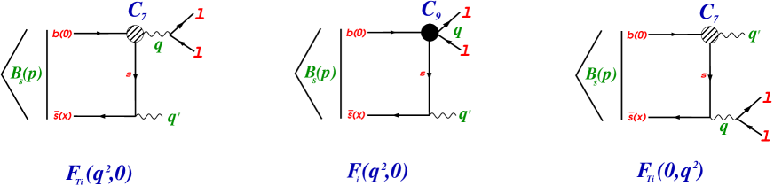
(a)                                             (b)                                             (c)

Fig. 1: Diagrams describing top-quark contributions to $\bar{B}_{s}\to\gamma l^{+}l^{-}$ amplitude. Dashed circle denotes the $O_{7}$ operator, solid circle - $O_{9}$ operator. Diagrams (a) and (b) describe the contribution $A^{(1)}$ where the real photon is emitted by spectator $s$-quark. Diagram (c) describes $A^{(2)}$ where the real photon is emitted from the penguin. We do not show $1/m_{b}$-suppressed diagrams where real or virtual photon is emitted by spectator $b$-quark, see mnk2018 for details.

II.2 Charm-quark contribution

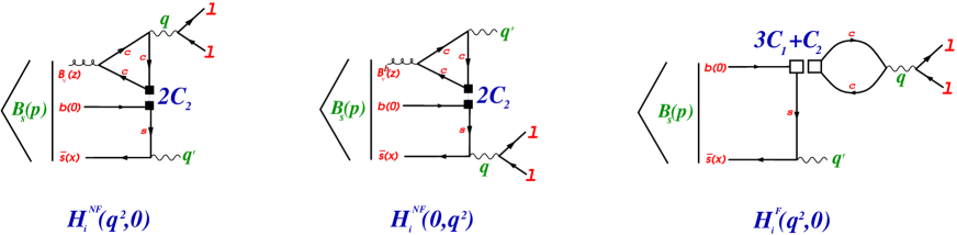
(a)                                             (b)                                             (c)

Fig. 2: The charm-loop contribution to the $B_{s}\to\gamma l^{+}l^{-}$ amplitude. (a) and (b) - nonfactorizable (NF) contributions induced by $H_{\rm eff}^{b\to s\bar{c}c[8\times 8]}$ (solid squares), (c) factorizable (F) contribution induced by $H_{\rm eff}^{b\to s\bar{c}c[1\times 1]}$ (empty squres); a similar factorizable contribution with the real photon emitted from the charm-quark loop vanishes and is not shown.

The charm-loop contribution to the $B_{s}\to\gamma l^{+}l^{-}$ amplitude,

$$A_{\rm charm}^{(\bar{B}_{s}\to\gamma ll)}=\langle\gamma(q^{\prime})l^{+}(p_{1})l^{-}(p_{2})|H_{\rm eff}^{b\to s\bar{c}c}|\bar{B}_{s}(p)\rangle,\qquad q=p_{1}+p_{2},$$ (2.12)

is described by the diagrams of Fig. 2. $H_{\rm eff}^{b\to s\bar{c}c}$ includes four-quark operators and may be written in the form

$$H_{\rm eff}^{b\to s\bar{c}c} = H_{\rm eff}^{b\to s\bar{c}c[1\times 1]}+H_{\rm eff}^{b\to s\bar{c}c[8\times 8]},$$ (2.13)

$$H_{\rm eff}^{b\to s\bar{c}c,[1\times 1]} = -\frac{G_{F}}{\sqrt{2}}\,V_{cb}V^{*}_{cs}\,\left(C_{1}+\frac{C_{2}}{3}\right)\bar{s}\gamma_{\mu}(1-\gamma_{5})b\cdot\bar{c}\gamma_{\mu}(1-\gamma_{5})c,$$ (2.14)

$$H_{\rm eff}^{b\to s\bar{c}c[8\times 8]} = -\frac{G_{F}}{\sqrt{2}}\,V_{cb}V^{*}_{cs}\,\left(2C_{2}\right)\,\bar{s}\gamma_{\mu}(1-\gamma_{5})t^{a}b\cdot\bar{c}\gamma_{\mu}(1-\gamma_{5})t^{a}c.$$ (2.15)

Let us introduce the amplitude of the transition into two virtual photons $\gamma^{\prime}$ and $\gamma$

$$A_{\rm charm}^{(\bar{B}_{s}\to\gamma^{\prime}\gamma)}=\langle\gamma^{\prime}(k^{\prime})\gamma(k)|H_{\rm eff}^{b\to s\bar{c}c}|\bar{B}_{s}(p)\rangle,\qquad p=k^{\prime}+k,$$ (2.16)

where the photon $\gamma^{\prime}(k^{\prime})$ is emitted by the $c$-quark, the photon $\gamma(k)$ is emitted from the $s$-quark and no symmetrization over photons is performed at this point (but is done later). The amplitude (2.16) may be written as mnk2018

$$\langle\gamma^{\prime}(k^{\prime})\gamma(k)|H_{\rm eff}^{b\to s\bar{c}c}|\bar{B}_{s}(p)\rangle=-\varepsilon_{\mu}(k^{\prime})\varepsilon_{\alpha}(k)H_{\mu\alpha}(k^{\prime},k),$$ (2.17)

with

$$H_{\mu\alpha}(k^{\prime},k)=i\int dxe^{ik^{\prime}x}\langle 0|T\left\{eQ_{c}\bar{c}(x)\gamma_{\mu}c(x),eQ_{s}\bar{s}(0)\gamma_{\alpha}s(0)\right\}|\bar{B}_{s}(p)\rangle,\qquad p=k+k^{\prime}.$$ (2.18)

Here quark fields are understood as Heisenberg field operators with respect to all SM interactions. The matrix element (2.18) has the Lorentz structure dictated by conservation of charm-quark and strange-quark vector currents that requires $k^{\alpha}H_{\mu\alpha}(k^{\prime},k)=0$ and $k^{\prime\mu}H_{\mu\alpha}(k^{\prime},k)=0$ (notice the absence of any contact terms):

$$H_{\mu\alpha}(k^{\prime},k)=-\frac{G_{F}}{\sqrt{2}}V_{cb}V^{*}_{cs}e^{2}\left[\epsilon_{\mu\alpha k^{\prime}k}H_{V}-i\left(g_{\alpha\mu}\,kk^{\prime}-k^{\prime}_{\alpha}k_{\mu}\right)H_{A}-i\left(k^{\prime}_{\alpha}-\frac{kk^{\prime}}{k^{2}}k_{\alpha}\right)\left(k_{\mu}-\frac{kk^{\prime}}{k^{\prime 2}}k^{\prime}_{\mu}\right)H_{3}\right],$$ (2.19)

with the invariant form factors $H_{i}$ depending on two variables, $H_{i}(k^{\prime 2},k^{2})$ ( $H_{i}$ include electric charges $Q_{s}$ and $Q_{c}$). The singularities in the projectors at $k^{2}=0$ and $k^{\prime 2}=0$ should not be the singularities of the amplitude $H_{\mu\alpha}(k^{\prime},k)$, leading to the constraints

$$H_{3}(k^{\prime 2}=0,k^{2})=H_{3}(k^{\prime 2},k^{2}=0)=0.$$ (2.20)

As the result, $H_{3}$ does not contribute to the $B_{s}\to\gamma l^{+}l^{-}$ amplitude: to obtain the latter, $H_{\mu\alpha}$ should be multiplied by either $\epsilon^{\alpha}(k)\bar{l}\gamma_{\mu}l$ or $\epsilon^{\mu}(k^{\prime})\bar{l}\gamma_{\alpha}l$. In each case, those terms in the $H_{3}$-part of $H_{\mu\alpha}$ containing $k^{\prime}_{\mu}$ or $k^{\prime}_{\alpha}$ vanish in the $B_{s}\to\gamma l^{+}l^{-}$ amplitude; the contribution of the “regular” structure $k_{\alpha}k_{\mu}$ also vanishes because the form factor $H_{3}=0$ if $k^{2}=0$ or $k^{\prime 2}=0$.

For the amplitude $A_{\rm charm}^{(\bar{B}_{s}\to\gamma ll)}$ we obtain

$$A_{\rm charm}^{(\bar{B}_{s}\to\gamma ll)}=-\frac{eQ_{l}}{q^{2}}\left\{H_{\mu\alpha}(q,q^{\prime})\bar{l}\gamma_{\mu}l\,\varepsilon_{\alpha}(q^{\prime})+H_{\mu\alpha}(q^{\prime},q)\varepsilon_{\mu}(q^{\prime})\,\bar{l}\gamma_{\alpha}l\right\},\qquad Q_{l}=-1.$$ (2.21)

II.3 Summing top and charm contributions

Adding charm contributions to the top contributions and taking into account that $V_{tb}V_{ts}^{*}\simeq-V_{cb}V_{cs}^{*}$ leads to the following simple modifications mnk2018 :

$$A^{(1)}_{i}(q^{2}) \to \frac{2C_{7}}{q^{2}}m_{b}\,F_{Ti}(q^{2},0)+C_{9}\frac{F_{i}(q^{2},0)}{M_{B}}+{8\pi^{2}}\frac{H_{i}(q^{2},0)}{q^{2}},$$

$$A^{(2)}_{i}(q^{2}) \to \frac{2C_{7}}{q^{2}}m_{b}\,F_{Ti}(0,q^{2})+8\pi^{2}\frac{H_{i}(0,q^{2})}{q^{2}},\qquad i=V,A.$$ (2.22)

The full amplitude is the sum of $A^{(1)}$ and $A^{(2)}$:

$$A_{i}(q^{2})=\frac{2C_{7}}{q^{2}}m_{b}\,\left(F_{Ti}(q^{2},0)+F_{Ti}(0,q^{2})\right)+C_{9}\frac{F_{i}(q^{2},0)}{M_{B}}+{8\pi^{2}}\frac{H_{i}(q^{2},0)+H_{i}(0,q^{2})}{q^{2}},\qquad i=V,A.$$ (2.23)

The functions $H_{i}(k^{\prime 2},k^{2})$ which contain factorizable and nonfactorizable charming loop contributions will be discussed in the next Section.

III Charming loop contributions to $B_{s}\to\gamma^{*}\gamma^{*}$

In Eq. (2.18), quark fields are the Heisenberg operators in the SM, i.e. the corresponding $S$-matrix includes weak interactions of quarks. So we need to expand the S-matrix to the first order in weak interaction.

III.1 Factorizable contribution of the charming loop

Factorizable contributions of the charming loop emerge in

$${\cal A}^{(\bar{B}_{s}\to\gamma^{\prime}\gamma)}_{\text{charm,F}}=\langle\gamma^{\prime}(k^{\prime}),\gamma(k)|H^{b\to s\bar{c}c[1\times 1]}_{\rm eff}|\bar{B}_{s}(p)\rangle,$$ (3.24)

when no gluons are exchanges between the charm-quark loop and the $B$-meson loop (whereas all gluon exchanges inside the loops are allowed). The corresponding $H^{\rm F}_{\mu\alpha}(k^{\prime},k)$ reads

$$H^{\rm F}_{\mu\alpha}(k^{\prime},k) = \frac{G_{F}}{\sqrt{2}}V_{cb}V_{cs}^{*}\frac{3C_{1}+C_{2}}{3}e\,Q_{c}\Pi^{cc}_{\mu\nu}(k^{\prime})\left(i\int dye^{ik^{\prime}y}\langle 0|T\left\{\bar{s}\gamma_{\nu}(1-\gamma_{5})b(y),e\,Q_{s}\,\bar{s}\gamma_{\alpha}s(0)\right\}|\bar{B}_{s}(p)\rangle\right),$$ (3.25)

where the expression in brackets is just the amplitude of (A.71) and

$$\Pi^{cc}_{\mu\nu}(k^{\prime})=i\int dxe^{ik^{\prime}x}\langle 0|T\{\bar{c}\gamma_{\mu}c(x),\bar{c}\gamma_{\nu}c(0)\}|0\rangle=\left(-g_{\mu\nu}k^{\prime 2}+k^{\prime}_{\mu}k^{\prime}_{\nu}\right)\Pi_{cc}(k^{\prime 2}).$$ (3.26)

For the invariant function $\Pi_{cc}(s)$ we may write the spectral representation with one subtraction

$$\Pi_{cc}(k^{\prime 2})=\Pi_{cc}(0)+\frac{k^{\prime 2}}{\pi}\int\frac{{\rm Im}\,\Pi_{cc}(s)}{s(s-k^{\prime 2})}ds,$$ (3.27)

At $k^{\prime 2}\ll 4m_{c}^{2}$, $\Pi_{cc}(k^{\prime 2})$ can be calculated in perturbative QCD. At leading order in $\alpha_{s}$, one finds

$${\rm Im}\,\Pi_{cc}(s)=\frac{N_{c}}{12\pi}\frac{2m_{c}^{2}+s}{s}\sqrt{1-\frac{4m_{c}^{2}}{s}},\qquad\Pi_{cc}(0)=\frac{9}{16\pi^{2}}\left\{-\frac{8}{9}\ln\left(\frac{m_{c}}{m_{b}}\right)-\frac{4}{9}\right\}.$$ (3.28)

The factorizable contributions to the form factors $H_{i}(k^{\prime 2},k^{2})$ are related to $f,a_{1},a_{2}$ (see Appendix A) as follows

$$H_{V}^{\rm F}(k^{\prime 2},k^{2}) = \frac{3C_{1}+C_{2}}{3}Q_{c}\,k^{\prime 2}\Pi_{\bar{c}c}(k^{\prime 2})2g(k^{\prime 2},k^{2}),$$ (3.29)

$$H_{A}^{\rm F}(k^{\prime 2},k^{2}) = \frac{3C_{1}+C_{2}}{3}Q_{c}\,k^{\prime 2}\Pi_{\bar{c}c}(k^{\prime 2})\frac{f(k^{\prime 2},k^{2})}{kk^{\prime}},$$ (3.30)

$$H_{3}^{\rm F}(k^{\prime 2},k^{2}) = \frac{3C_{1}+C_{2}}{3}Q_{c}\,k^{\prime 2}\Pi_{\bar{c}c}(k^{\prime 2})\left\{\frac{f}{kk^{\prime}}+a_{1}+a_{2}\right\}.$$ (3.31)

Obviously, $H_{V,A,3}^{\rm F}(k^{\prime 2}=0,k^{2})=0$. Therefore, the factorizable $\bar{c}c$ contribution to the amplitude $A^{(2)}$ vanish; the $\bar{c}c$ contributions to $A^{(2)}$ comes exclusively from NF gluon exchanges. The factorizable contribution to $A^{(1)}$ takes the form [$H^{\rm F}_{3}(k^{\prime 2},k^{2}=0)=0$ because of the constraint (A.73)]:

$$H_{i}^{\rm F}(q^{2},0) = \frac{3C_{1}+C_{2}}{3}\,Q_{c}\,q^{2}\Pi_{\bar{c}c}(q^{2})\frac{F_{i}(q^{2},0)}{M_{B}},\quad i=A,V$$ (3.32)

Since $3C_{1}+C_{2}<0$ and for the $B_{s}\to\gamma$ transition $F_{V,A}(q^{2},0)>0$ mnk2018 , we find that $H_{V,A}^{\rm F}(q^{2},0)<0$ at $q^{2}>0$.

Clearly, the factorizable $\bar{c}c$ contributions to $A^{(1)}$ can be described as a universal $q^{2}$-addition to the coefficient $C_{9}$:

$$C_{9}\to C^{\rm eff}_{9}(q^{2})=C_{9}+\Delta^{\rm F}C_{9}(q^{2}),\quad\Delta^{\rm F}C_{9}(q^{2})=8\pi^{2}Q_{c}\frac{3C_{1}+C_{2}}{3}\Pi_{\bar{c}c}(q^{2}).$$ (3.33)

Taking into account that $C_{9}$, $C_{2}$ and $3C_{1}+C_{2}$ have the same sign, and $\Pi_{\bar{c}c}(q^{2})\geq 0$, we find that

$$\delta^{\rm F}C_{9}(q^{2})\equiv\Delta^{\rm F}C_{9}(q^{2})/C_{9}>0.$$ (3.34)

III.2 Non-factorizable contribution of the charming loop

Non-factorizable (NF) contributions of the charming loop emerge in

$${\cal A}^{(\bar{B}_{s}\to\gamma^{\prime}\gamma)}_{\text{charm,NF}}=\langle\gamma^{\prime}(k^{\prime}),\gamma(k)|H^{b\to s\bar{c}c[8\times 8]}_{\rm eff}|\bar{B}_{s}(p)\rangle.$$ (3.35)

The corresponding $H_{\mu\alpha}^{\rm NF}$ has the form

$$H^{\rm NF}_{\mu\alpha}(k^{\prime},k) = i^{3}\frac{G_{F}}{\sqrt{2}}V_{cb}V_{cs}^{*}e^{2}(2C_{2})Q_{c}Q_{s}\int dzdxdye^{ik^{\prime}z}e^{iky}$$ (3.36)

$$\times\langle 0|T\Big{\{}\bar{c}\gamma_{\mu}c(z),\bar{c}(0)t^{a}\gamma_{\beta}(1-\gamma_{5})c(0),\bar{c}(x)t^{b}\gamma_{\nu}c(x)\Big{\}}|0\rangle$$

$$\times\langle 0|T\Big{\{}\bar{s}(y)\gamma_{\alpha}s(y),\bar{s}(0)t^{a}\gamma_{\beta}(1-\gamma_{5})b(0)g_{s}B^{b}_{\nu}(x)\Big{\}}|\bar{B}_{s}(p)\rangle.$$

This expression takes into account photon emission by the $B$-meson valence $s$-quark; a $1/m_{b}$-suppressed contribution related to photon emission by the valence $b$-quark will be omitted. We now outline the procedure of calculating $H^{\rm NF}_{\mu\alpha}$ and for all details refer to our recent paper bbm2023 .

$\bullet$ The amplitude Eq. (3.36) includes the charm-quark loop contribution described by the $\langle VVA\rangle$ three-point function:

$$\Gamma_{cc}^{\beta\nu\mu\,(ab)}\left(\kappa,k^{\prime}\right)=\int dx^{\prime}dz\>e^{ik^{\prime}z+i\kappa x^{\prime}}\langle 0|T\{\bar{c}(z)\gamma^{\mu}c(z),\bar{c}(0)\gamma^{\beta}(1-\gamma_{5})t^{a}c(0),\bar{c}(x^{\prime})\gamma^{\nu}t^{b}c(x^{\prime})\}|0\rangle=\frac{1}{2}\delta^{ab}\,\Gamma_{cc}^{\beta\nu\mu}(\kappa,k^{\prime}),$$ (3.37)

where $k^{\prime}$ is the momentum of the external virtual photon (vertex containing index $\mu$) and $\kappa$ is the gluon momentum (vertex containing index $\nu$). Here $t^{c}$, $c=1,\dots,8$ are $SU_{c}(3)$ generators normalized as ${\rm Tr}(t^{a}t^{b})=\frac{1}{2}\delta^{ab}$.

The octet current $\bar{c}(0)\gamma^{\beta}(1-\gamma_{5})t^{a}c(0)$ is a charm-quark part of the octet-octet weak Hamiltonian. Taking into account vector-current conservation, it is convenient to parametrize $\Gamma_{cc}^{\beta\nu\mu}(\kappa,k^{\prime})$ as follows lm

$$\Gamma_{cc}^{\beta\nu\mu}(\kappa,k^{\prime})=-i\left(\kappa^{\beta}+k^{\prime\beta}\right)\epsilon^{\nu\mu\kappa k^{\prime}}\,F_{0}-i\left(k^{\prime 2}\epsilon^{\beta\nu\mu\kappa}-k^{\prime\mu}\epsilon^{\beta\nu k^{\prime}\kappa}\right)\,F_{1}-i\left(\kappa^{2}\epsilon^{\beta\mu\nu k^{\prime}}-\kappa^{\nu}\epsilon^{\beta\mu\kappa k^{\prime}}\right)\,F_{2}.$$ (3.38)

The form factors $F_{0,1,2}$ are functions of three independent invariant variables $k^{\prime 2}$, $\kappa^{2}$, and $\kappa k^{\prime}$. We use a convenient representation of the one-loop form factors in the form bbm2023

$$F_{i}\left(\kappa^{2},\kappa k^{\prime},k^{\prime 2}\right) = \frac{1}{\pi^{2}}\int\limits_{0}^{1}d\xi\int\limits_{0}^{1-\xi}d\eta\frac{\Delta_{i}(\xi,\eta)}{m_{c}^{2}-2\,\xi\eta\>\kappa k^{\prime}-\xi(1-\xi)k^{\prime 2}-\eta(1-\eta)\kappa^{2}},\quad i=0,1,2,$$ (3.39)

$$\Delta_{0}=-\xi\eta,\quad\Delta_{1}=\xi(1-\eta-\xi),\quad\Delta_{2}=\eta(1-\eta-\xi).$$

As shown in Sect. III of bbm2023 , the operator describing the contribution of the charm-quark loop may be written in the form containing only $G^{a}_{\nu\alpha}$:

$$\int d\kappa e^{-i\kappa x~{}}\Gamma_{cc}^{\beta\nu\mu\,(ab)}(\kappa,k^{\prime})B^{b}_{\nu}(x)dx=\frac{1}{4}\int d\kappa e^{-i\kappa x~{}}{\overline{\Gamma}}_{cc}^{\beta\nu\mu\xi}(\kappa,k^{\prime})G^{a}_{\nu\xi}(x)dx$$ (3.40)

with

$${\overline{\Gamma}}_{cc}^{\beta\nu\mu\xi}(\kappa,k^{\prime})=\left(\kappa^{\beta}+k^{\prime\beta}\right)\epsilon^{\nu\mu\xi k^{\prime}}\,F_{0}+\left(k^{\prime\mu}\epsilon^{\beta\nu\xi k^{\prime}}+k^{\prime 2}\epsilon^{\beta\nu\mu\xi}\right)\,F_{1}+\left(\kappa^{\beta}\epsilon^{\xi\nu\mu k^{\prime}}+\kappa^{\mu}\epsilon^{\xi\beta\nu k^{\prime}}-\kappa k^{\prime}\,\epsilon^{\xi\beta\nu\mu}\right)\,F_{2}.$$ (3.41)

$\bullet$ Making use of this result for the charm-quark $\langle VVA\rangle$ triangle, we have

$$H^{\rm NF}_{\mu\alpha} = -\frac{G_{F}}{\sqrt{2}}V_{cb}V^{*}_{cs}e^{2}(2C_{2})Q_{s}Q_{c}\,\tilde{H}^{\rm NF}_{\mu\alpha}(k^{\prime},k),$$ (3.42)

$$\tilde{H}^{\rm NF}_{\mu\alpha}(k^{\prime},k) = \frac{1}{4(2\pi)^{8}}\int d\tilde{k}dye^{-i(\tilde{k}-k)y}dxd\kappa e^{-i\kappa x}\overline{\Gamma}_{cc}^{\beta\nu\mu\xi}(\kappa,k^{\prime})\langle 0|\bar{s}(y)\gamma^{\eta}\frac{\tilde{\not{k}}+m_{s}}{m_{s}^{2}-\tilde{k}^{2}}\gamma^{\mu}(1-\gamma^{5})t^{b}G^{b}_{\nu\xi}(x)b(0)|\bar{B}_{s}(p)\rangle.$$

(3.43)

For $k^{\prime 2}=0$ or $k^{2}=0$, $\tilde{H}^{\rm NF}_{\mu\alpha}$ contains 2 form factors

$$\tilde{H}^{\rm NF}_{\mu\alpha}(k^{\prime},k)=\tilde{H}^{\rm NF}_{V}\epsilon_{\mu\alpha k^{\prime}k}-i\tilde{H}^{\rm NF}_{A}\left(g_{\rho\eta}\,k^{\prime}k-k_{\mu}k^{\prime}_{\alpha}\right),$$ (3.44)

such that

$$H_{i}^{\rm NF}(k^{\prime 2},k^{2})=2C_{2}Q_{s}Q_{c}\tilde{H}_{i}^{\rm NF}(k^{\prime 2},k^{2}).$$ (3.45)

$\bullet$ The $B$-meson structure contributes to ${H}^{\rm NF}_{\mu\alpha}$ via the full set of 3BS

$$\langle 0|\bar{s}(y)\Gamma_{i}t^{a}b(0)G^{a}_{\nu\alpha}(x)|\bar{B}_{s}(p)\rangle,$$ (3.46)

with $\Gamma_{i}$ the appropriate combinations of $\gamma$-matrices. This quantity is not gauge invariant, since it contains field operators at different locations. To make it gauge-invariant, one needs to insert Wilson lines between the field operators. To simplify the full consideration, it is convenient to work in a fixed-point gauge, where the Wilson lines reduce to unity factors.

When the coordinates $x$ and $y$ are independent variables, the 3BS has the following decomposition bbm2023 :

$$\langle 0|\bar{s}(y)G_{\nu\xi}(x)\Gamma\,b(0)|\bar{B}_{s}(p)\rangle=\frac{f_{B}M_{B}^{3}}{4}\int D(\omega,\lambda)\,e^{-i\lambda yp-i\omega xp}\,{\rm Tr}\Bigg{\{}\gamma_{5}\Gamma\,(1+\not{v})$$

$$\times\bigg{[}(p_{\nu}\gamma_{\xi}-p_{\xi}\gamma_{\nu})\frac{1}{M_{B}}[\Psi_{A}-\Psi_{V}]-i\sigma_{\nu\xi}\Psi_{V}$$

$$-\frac{(x_{\nu}p_{\xi}-x_{\xi}p_{\nu})}{xp}\left(X_{A}^{(x)}+\frac{\not{x}}{xp}M_{B}W^{(x)}\right)+\frac{(x_{\nu}\gamma_{\xi}-x_{\xi}\gamma_{\nu})}{xp}M_{B}\left(Y^{(x)}_{A}+W^{(x)}+\frac{\not{x}}{xp}M_{B}Z^{(x)}\right)$$

$$-\frac{(y_{\nu}p_{\xi}-y_{\xi}p_{\nu})}{yp}\left(X_{A}^{(y)}+\frac{\not{y}}{yp}M_{B}W^{(y)}\right)+\frac{(y_{\nu}\gamma_{\xi}-y_{\xi}\gamma_{\nu})}{yp}M_{B}\left(Y^{(y)}_{A}+W^{(y)}+\frac{\not{y}}{yp}M_{B}Z^{(y)}\right)$$

$$-i\epsilon_{\nu\xi\mu\beta}\,\frac{x^{\mu}p^{\beta}}{xp}\gamma^{5}\tilde{X}^{(x)}_{A}+i\epsilon_{\nu\xi\mu\beta}\,\frac{x^{\mu}\gamma^{\beta}}{xp}\gamma^{5}M_{B}\tilde{Y}^{(x)}_{A}-i\epsilon_{\nu\xi\mu\beta}\,\frac{x^{\mu}p^{\beta}}{xp}\gamma^{5}\tilde{X}^{(y)}_{A}+i\epsilon_{\nu\xi\mu\beta}\,\frac{x^{\mu}\gamma^{\beta}}{xp}\gamma^{5}M_{B}\tilde{Y}^{(y)}_{A}\bigg{]}\Bigg{\}},$$ (3.47)

where

$$D(\omega,\lambda)=d\omega d\lambda\theta(\omega)\theta(\lambda)\theta(1-\omega-\lambda)$$ (3.48)

takes into account rigorous constraints on the variables $\omega$ and $\lambda$. All invariant amplitudes $\Phi=\Psi_{A},\Psi_{V},\dots$ are functions of 5 variables, $\Phi(\omega,\lambda,x^{2},y^{2},xy)$, for which we may write Taylor expansion in $x^{2},y^{2},xy$. Here we limit our analysis to zero-order terms in this expansion. The corresponding zero-order terms in $\Phi$’s are functions of dimensionless arguments $\lambda$ and $\omega$ and are referred to as the Lorentz 3DAs.

The normalization conditions for $\Psi_{A}$ and $\Psi_{V}$ have the form braun2017 :

$$\int D(\omega,\lambda)\,\Psi_{A}\left(\omega,\lambda\right)=\frac{\lambda_{E}^{2}}{3M_{B}^{2}},\qquad\int D(\omega,\lambda)\,\Psi_{V}\left(\omega,\lambda\right)=\frac{\lambda_{H}^{2}}{3M_{B}^{2}}.$$ (3.49)

A number of Lorentz structures in (III.2) contain singularities at $xp=0$ and $yp=0$. Since 3BS (III.2) is a continuous regular function at the point $x^{2}=0$, $y^{2}=0$, $xp=0$, $yp=0$, the absence of singularities at $xp\to 0$ and $yp\to 0$ leads to a number of constraints on the corresponding 3DAs m2023 : namely, the primitives of these 3DAs should vanish at the boundaries of the 3DA support regions. The appropriate modifications of 3DAs at the upper end-point region of $\omega$ and $\lambda$ have been developed in bbm2023 . Here we follow the approach of bbm2023 and refer to that publication for details.

$\bullet$ Making use of Eq. (III.2) (i) reduces the matrix element in Eq. (3.43) to trace calculation and (ii) reduces the integrations over $x$ and $y$ to $\delta(\kappa+\omega p)\delta(\tilde{k}-k+\lambda p)$ (see details in bbm2023 ). Using these $\delta$-functions to integrate over $\kappa$ and $k$, the form factors $H_{i}$, $i={A,V}$ are obtained as integrals of the form

$$\tilde{H}^{\rm NF}_{i}(k^{\prime 2},k^{2})=\int\limits_{0}^{2\omega_{0}}d\omega\int\limits_{0}^{2\omega_{0}-\omega}d\lambda\int\limits_{0}^{1}d\xi\int\limits_{0}^{1-\xi}d\eta\;\tilde{h}^{\rm NF}_{i}(\omega,\lambda,\xi,\eta\,|\,k^{\prime 2},k^{2}).$$ (3.50)

Here $\tilde{h}_{i}$ are linear combinations of the 3DAs entering Eq. (III.2 and their primitives, and include the form factors $F_{0,1,2}$ describing the charming $\langle VVA\rangle$ triangle and the $s$-quark propagator. As an illustration, we present the leading part of the $\psi_{A}$ and $\psi_{V}$ contribution to $\tilde{h}_{V}^{\rm NF}(k^{\prime 2},k^{2})$ [neglecting in the numerator all powers of $\lambda=O(\Lambda_{\rm QCD}/m_{b})$ and $\omega=O(\Lambda_{\rm QCD}/m_{b})$]

$$\tilde{h}_{V}(\omega,\lambda,\xi,\eta\,|\,k^{\prime 2},k^{2}) = -\frac{\frac{1}{2}f_{B}M^{4}_{B}}{m_{s}^{2}+\lambda(1-\lambda)M_{B}^{2}-(1-\lambda)k^{2}-\lambda k^{\prime 2}}$$ (3.51)

$$\times\left\{(\Psi_{A}+\Psi_{V})\left[(M_{B}^{2}+k^{\prime 2}-k^{2})F_{0}-2k^{\prime 2}F_{1}\right]-2\Psi_{A}k^{\prime 2}\left[F_{0}-3F_{1}\right]\right\}.$$

The form factors $F_{0,1,2}$ given by Eq. (3.39) depend on $\xi$ and $\eta$ and should be evaluated for $\kappa=-\omega p$. Notice that $F_{0}<0$ and thus $\tilde{H}_{V}(k^{\prime 2},k^{2})>0$; the form factor $\tilde{H}_{A}(k^{\prime 2},k^{2})$ turns out numerically close to $\tilde{H}_{V}(k^{\prime 2},k^{2})$.

IV Results for the $B_{s}\to\gamma l^{+}l^{-}$ NF charming loop form factors

Our further calculation directly follows the approach of bbm2023 with the difference that now both photons are virtual.

IV.1 Model for 3DAs

Following bbm2023 , we make use of the set of 3DAs of local-duality (LD) model of braun2017 ; wang2019 and perform the appropriate modifications of the 3DAs $X_{A}^{(x)}$, $X_{A}^{(y)}$, …. All necessary details including the explicit expressions of the 3DAs are given in Section IV of bbm2023 and will not be repeated here. As a reference, we present just the Lorentz 3DAs $\Psi_{A}$ and $\Psi_{V}$ of the LD model braun2017 :

$$\Psi_{A}(\omega,\lambda) = (\phi_{3}+\phi_{4})/2,$$

$$\Psi_{V}(\omega,\lambda) = (-\phi_{3}+\phi_{4})/2$$ (4.52)

with

$$\phi_{3} = \frac{105(\lambda_{E}^{2}-\lambda_{H}^{2})}{32\omega_{0}^{7}M_{B}^{2}}\,\lambda\omega^{2}\left(2\omega_{0}-\omega-\lambda\right)^{2}\theta\left(2\omega_{0}-\omega-\lambda\right),$$ (4.53)

$$\phi_{4} = \frac{35(\lambda_{E}^{2}+\lambda_{H}^{2})}{32\omega_{0}^{7}M_{B}^{2}}\,\omega^{2}\left(2\omega_{0}-\omega-\lambda\right)^{3}\theta\left(2\omega_{0}-\omega-\lambda\right).$$ (4.54)

Dimensionless parameter $\omega_{0}$ is related to $\lambda_{B}$, the inverse moment of the $B$-meson LC distribution amplitude, as

$$\omega_{0}=\frac{5}{2}\frac{\lambda_{B}}{M_{B}}.$$ (4.55)

For this model, the integration limits take the following form ($2\omega_{0}<1$):

$$\int D(\omega,\lambda)\,\theta\left(2\omega_{0}-\omega-\lambda\right)\,{(\dots)}=\int\limits_{0}^{2\omega_{0}}d\omega\int\limits_{0}^{2\omega_{0}-\omega}d\lambda\,{(\dots)}.$$ (4.56)

The form factors $H_{A,V}(k^{\prime 2},k^{2})$ have explicit linear dependence on $\lambda_{E,H}^{2}$, so we write

$$H^{\rm NF}_{i}(k^{\prime 2},k^{2})=2C_{2}Q_{s}Q_{c}\left[R_{iE}(k^{\prime 2},k^{2})\lambda_{E}^{2}+R_{iH}(k^{\prime 2},k^{2})\lambda_{H}^{2}\right],\qquad i=A,V.$$ (4.57)

QCD sum rules suggest an approximate relation braun2017

$$\lambda_{H}^{2}\simeq 2\lambda_{E}^{2}.$$ (4.58)

Then, the appropriate combinations of the form factors which describe NF charm contributions have the form

$$R_{i}(k^{\prime 2},k^{2})=R_{iE}(k^{\prime 2},k^{2})+2R_{iH}(k^{2},k^{2}),\qquad H_{i}(k^{\prime 2},k^{2})=2C_{2}Q_{s}Q_{c}\lambda_{E}^{2}R_{i}(k^{\prime 2},k^{2}),\qquad i=A,V.$$ (4.59)

Combining (4.58) with QCD equations of motion, 3BS model used in our analysis leads to approximate relations

$$\lambda_{H}^{2}\simeq 1.2\lambda_{B_{s}}^{2},\qquad\lambda_{E}^{2}\simeq 0.6\lambda_{B_{s}}^{2}.$$ (4.60)

This leads to an explicit linear dependence of $H_{i}$ on $\lambda_{B_{s}}^{2}$. It should be noticed however that the form factors have also a complicated implicit dependence on $\lambda_{B_{s}}$ through a $\lambda_{B_{s}}$-dependent shape of the three-particle distribution amplitudes of $B_{s}$. We present below our results for the benchmark point bbm2023

$$\lambda_{B_{s}}(1\;{\rm GeV})=0.45\;{\rm GeV}.$$ (4.61)

For a discussion of the existing estimates of $\lambda_{B_{s}}$ we refer to khodjamirian2020 ; kou ; braun2004 ; beneke2011 ; zwicky2021 ; im2022 .

IV.2 Results for the form factors $H^{\rm NF}_{i}(k^{\prime 2},k^{2})$

The analytic expressions (3.50) are based on finite-order QCD diagrams and thus cannot be trusted near quark thresholds. For instance, the calculated form factors exhibit steep rise at negative $k^{2}\to 0$ which is unphysical, as the nearest hadron pole lies at $k^{2}=M_{\phi}^{2}$ and the two-meson threshold lies at $k^{2}=4M_{K}^{2}$.

We therefore pursue the strategy previously applied in ms2000 ; bbm2023 to the form factors of one variable, and extend it to the case of $R_{i}(k^{\prime 2},k^{2})$ depending on two variables: We first calculate the form factors $R_{i}(k^{\prime 2},k^{2})$ using the analytic expressions (3.50) in the rectangular region relatively far from quark thresholds in QCD diagrams:

$$\qquad 0<k^{\prime 2}({\rm GeV}^{2})<4,\quad-5<k^{2}({\rm GeV}^{2})<-0.6.$$ (4.62)

We then interpolate the results obtained in this region as function of two variables $k^{\prime 2}$ and $k^{2}$ by a formula which takes into account the correct location of the hadron poles at $k^{\prime 2}=M_{J/\psi}^{2}$ and $k^{2}=M_{\phi}^{2}$ and contains a number of fit parameters allowing to fit $R_{i}(k^{\prime 2},k^{2})$ in the rectangular region (4.62) with an accuracy of not worse than 2 percent. Finally, since our interpolating formula takes into account correct location of the lowest meson poles in the $k^{\prime 2}$ and $k^{2}$ channels, we find it eligible to use this formula to extrapolate the form factors to the region of timelike momenta $k^{\prime 2}\leq M^{2}_{J/\psi}$ and $k^{2}\leq 4M_{K}^{2}$.

Fig. 3 shows our numerical predictions for the NF form factors corresponding to the central values of all parameters, for the discussion we refer to bbm2023 . As reported in bbm2023 , the accuracy of the predictions for the form factors depend sizebly on $\lambda_{B_{s}}$. However, for a given value of $\lambda_{B_{s}}$, the form factors $H_{i}(k^{\prime 2},k^{2})$ may be calculated with an accuracy around 10%.

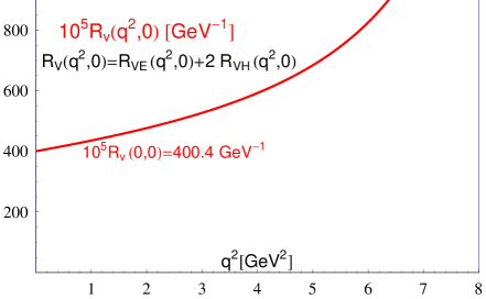
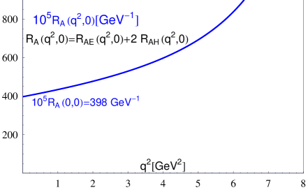
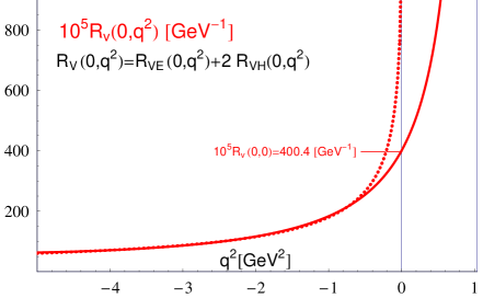
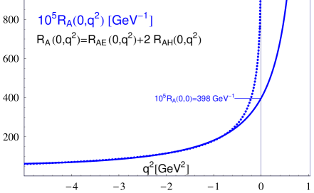
Fig. 3: Solid lines are the fits. For $R(0,q^{2})$, dashed lines present the results of direct calculations.

IV.3 NF charm vs top

The effect of factorizable charming loops may be conveniently described as a process-independent but $q^{2}$-dependent correction to the Wilson coefficient $C_{9}$, Eq. (3.33), with $\delta^{\rm F}C_{9}(q^{2})>0$.

One may in principle describe also NF charming-loop contribution as a correction to $C_{9}$; in this case, however, the correction explodes at small $q^{2}$. So it is more natural to describe the effect of NF charm in $B_{s}\to\gamma ll$ as additions to the Wilson coefficient $C_{7}$ related to different $A_{i}(q^{2})$ ($i=A,V$) in Eq. (2.23):

$$A_{V}(q^{2}): C_{7}\to C_{7}+\Delta^{\rm NF}_{V}C_{7}(q^{2}),$$

$$A_{A}(q^{2}): C_{7}\to C_{7}+\Delta^{\rm NF}_{A}C_{7}(q^{2}),$$ (4.63)

with the relative correction

$$\delta^{\rm NF}_{i}C_{7}(q^{2})=\frac{\Delta^{\rm NF}_{i}C_{7}(q^{2})}{C_{7}}=8\pi^{2}\,Q_{s}Q_{c}\frac{C_{2}}{C_{7}}\frac{1}{m_{b}}\frac{\tilde{H}^{\rm NF}_{i}(q^{2},0)+\tilde{H}^{\rm NF}_{i}(0,q^{2})}{F_{Ti}(q^{2},0)+F_{Ti}(0,q^{2})},\qquad i=A,V.$$ (4.64)

The Wilson coefficients $C_{2}$ and $C_{7}$ have opposite signs, $\tilde{H}^{\rm NF}_{i}(q^{2},0)$ and $\tilde{H}^{\rm NF}_{i}(0,q^{2})$ as well as $F_{Ti}(q^{2},0)$ and $F_{Ti}(0,q^{2})$ are positive mnk2018 . So, the relative correction $\delta^{\rm NF}_{i}C_{7}$ is found to be positive

$$\delta^{\rm NF}_{i}C_{7}(q^{2})>0.$$ (4.65)

Numerically, $\delta^{\rm NF}_{A}C_{7}(q^{2})\simeq\delta^{\rm NF}_{V}C_{7}(q^{2})$. The form factors $H_{i}(q^{2},0)$ are predicted in the region $q^{2}<M^{2}_{J/\psi}$, whereas $H_{i}(0,q^{2})$ is predicted in the region $q^{2}<4M^{2}_{K}$ [Recall that at $q^{2}>4M^{2}_{K}$, $H_{i}(0,q^{2})$ have imaginary part]. In principle, one can model $H_{i}(0,q^{2})$ for $q^{2}>4M^{2}_{K}$, but this interesting problem is beyond the scope of this paper. So, Fig. 4(a) presents $\delta^{\rm NF}_{i}C_{7}(q^{2})$ in the range $0<q^{2}<4M^{2}_{K}$, where our predictions are less model dependent. On the other hand, as the analysis of mnk2018 has shown, for $q^{2}\geq 3$ GeV² (i.e., far above $M_{\phi}^{2}$), the contribution of the amplitude $H^{\rm NF}_{i}(0,q^{2})$ turns out to be much suppressed compared to $H^{\rm NF}_{i}(q^{2},0)$. The same occurs for the form factor $F_{Ti}$: in this range of $q^{2}$, $F_{Ti}(q^{2},0)\gg F_{Ti}(0,q^{2})$. Therefore the contribution of $H^{\rm NF}_{i}(0,q^{2})$ in the numerator and the contribution of $F_{Ti}(0,q^{2})$ in the denominator of (4.64) may be neglected (one however might need to be careful as both $H^{\rm NF}_{i}(0,q^{2})$ and $H^{\rm NF}_{i}(0,q^{2})$ have imaginary parts at $q^{2}>4M_{K}^{2}$). Then the main contribution to $\delta^{\rm NF}C_{7}(q^{2})/C_{7}$ in this range of $q^{2}$ is expected to come from the ratio $\frac{H^{\rm NF}_{i}(q^{2},0)}{F_{Ti}(q^{2},0)}$. This contribution is denoted as

$$\delta^{\rm NF}_{i}C_{7}(q^{2},0)=\Delta^{\rm NF}_{i}C_{7}(q^{2},0)/C_{7},$$ (4.66)

and is shown in Fig. 4(b) for $i=V$.

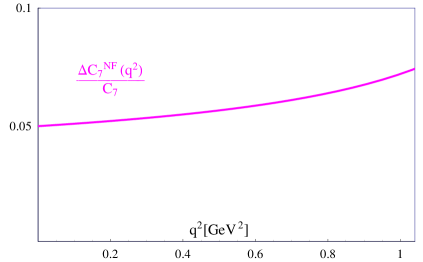
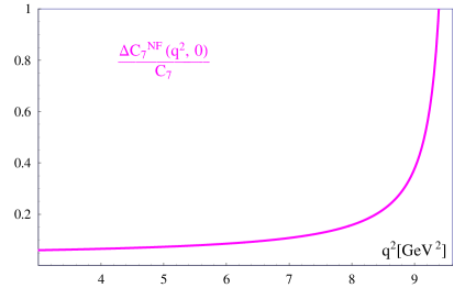
(a)	(b)

Fig. 4: (a) The relative NF correction $\delta^{\rm NF}_{V}C_{7}(q^{2})$ given by Eq. (4.64). (b) $\delta^{\rm NF}C_{7}(q^{2},0)$ given by Eq. (4.64) which dominates in $\delta^{\rm NF}_{V}C_{7}(q^{2})$ for $q^{2}>3{\rm GeV}^{2}$

Closing this Section, we would like to emphasize that factorizable and nonfactorizable contributions of the charming loops, $H_{i}^{\rm F}$ and $H_{i}^{\rm NF}$, have opposite signs.

V Discussion and conclusions

This paper extended the theoretical approach to NF charming loops in FCNC $B_{s}$ decays recently formulated in bbm2023 and for the first time reports the results for NF charm in $B_{s}\to\gamma ll$ decays:

(i) We derived analytical expressions for the form factors $H_{i}^{\rm NF}(k^{\prime 2},k^{2})$, $i=A,V$, describing NF contribution of charming loops to the amplitude of the $B_{s}$ meson transition into two virtual photons (the first argument, $k^{\prime 2}$ corresponds to the momentum emitted from the charming loop, whereas the second argument, $k^{2}$, corresponds to the momentum emitted by the valence $s$-quark of the $B_{s}$-meson). These expressions may be written in the form

$$H_{i}^{\rm NF}(k^{\prime 2},k^{2})=2C_{2}Q_{s}Q_{c}\left[\lambda_{E}^{2}R_{iE}(k^{\prime 2},k^{2})+\lambda_{H}^{2}R_{iH}(k^{\prime 2},k^{2})\right]\qquad i=A,V,3.$$ (5.67)

Since an approximate relation $\lambda_{H}^{2}\simeq 2\lambda_{E}^{2}$ is expected, the linear combination

$$R_{i}(k^{\prime 2},k^{2})=2R_{iH}(k^{\prime 2},k^{2})+R_{iE}(k^{\prime 2},k^{2})$$ (5.68)

is approprate for the description of NF charming loops in $B_{s}$ decays such that

$$H_{i}^{\rm NF}(k^{\prime 2},k^{2})=2C_{2}Q_{s}Q_{c}\lambda_{E}^{2}R_{i}(k^{\prime 2},k^{2}).$$ (5.69)

We emphasize that according to our analysis, $R_{i}(k^{\prime 2},k^{2})>0$ in the region $k^{\prime 2}<M_{J/\psi}^{2}$ and $k^{2}<M_{\phi}^{2}$ and thus $H_{i}^{\rm NF}(k^{\prime 2},k^{2})$ is positive in this region. Recall that the factorizable contribution $H_{i}^{\rm F}(k^{\prime 2},k^{2})$ is negative.

(ii) The analytic expressions allow one to calculate the form factors $R_{i}(k^{\prime 2},k^{2})$ in a broad range $k^{\prime 2}<4m_{c}^{2}$ and $k^{2}<0$. However, calculations based on finite-order QCD diagrams are not expected to provide good description of the physical hadron amplitudes near quark thresholds (for instance, the calculated form factors exhibit steep rise at $k^{2}\to 0$ which is unphysical, as the nearest meson pole lies at $k^{2}=M_{\phi}^{2}$ and the two-meson threshold lies at $k^{2}=4M_{K}^{2}$). So we pursue the following strategy: We make use of the results of our calculation in the rectangular region $0<k^{\prime 2}({\rm GeV}^{2})<4$ and $-5<k^{2}({\rm GeV}^{2})<-0.6$ (i.e., sufficiently far from quark thresholds) and interpolate them by a simple analytic formula depending on $k^{\prime 2}$ and $k^{2}$, which takes into account the presence of the poles at $k^{\prime 2}=M_{J/\psi}^{2}$ and $k^{2}=M_{\phi}^{2}$. Numerical parameters in this formula are obtained by the fit to the results of our calculations and interpolate them with a 2% accuracy in the rectangular region mentioned above. The corresponding easy-to-use fit formulas for $R_{i}(k^{\prime 2},k^{2})$ are presented in Appendix C.

(iii) Since the interpolating formulas exhibit the correct location of the lowest hadron singularities, i.e., poles at $k^{\prime 2}=M_{J/\psi}^{2}$ and at $k^{2}=M_{\phi}^{2}$, our fit formulas are expected to provide reliable theoretical predictions for the form factors in a broader range $0<k^{\prime 2}<M_{J/\psi}^{2}$ and $-5\,{\rm GeV}^{2}<k^{\prime 2}<M_{\phi}^{2}$. Fig. 3 shows $R_{i}(0,q^{2})$ and $R_{i}(q^{2},0)$ related to $B_{s}\to\gamma ll$ decays.

(iv) The contribution of factorizable charm in $B_{s}\to\gamma ll$ decay may be treated as the $q^{2}$-dependent correction to the Wilson coefficient $C_{9}$, such that $\Delta^{\rm F}C_{9}(q^{2})/C_{9}>0$ at $q^{2}<M_{J/\psi}^{2}$. At the same time, the contribution of nonfactorizable charm in $B_{s}\to\gamma ll$ decay may be conveniently treated as the $q^{2}$-correction to the Wilson coefficient $C_{7}$, such that $\Delta^{\rm NF}C_{7}(q^{2})/C_{7}>0$ at $q^{2}<4M_{K}^{2}$ (at higher values of $q^{2}$ the physical NF charming loop has imaginary part). Fig. 4 presents our prediction for these quantities.

(v) Our numerical results for the form factors $H^{\rm NF}_{i}(k^{\prime 2},k^{2})$ depend sizeably on the precise value of the parameter $\lambda_{B_{s}}$. In this respect we see the same picture as for the $B_{s}\to\gamma\gamma$ decay, Fig. 7 in bbm2023 . And, similar to the form factors for $B_{s}\to\gamma\gamma$ decay, for a fixed value of $\lambda_{B_{s}}$, $H^{\rm NF}_{i}(k^{\prime 2},k^{2})$ may be calculated with about 10% accuracy.

It might be useful to recall that the $B_{s}\to\gamma ll$ decay amplitude receives contributions from the weak-annihilation type diagrams wa1 ; wa2 ; wa3 ; wang2024 . The weak-annihilation mechanism differs very much from the mechanism discussed in this paper and is therefore beyond the scope of our interest here. However, weak-annihilation diagrams should be taken into account in a complete analysis of $B_{s}\to\gamma ll$ decays.

Acknowledgments. We are pleased to express our gratitude to Yu-Ming Wang for his illuminating remarks and comments and to Otto Nachtmann, Hagop Sazdjian, and Silvano Simula for valuable discussions. D. M. gratefully acknowledges participation at the Erwin Schrödinger Institute (ESI) thematic program “Quantum Field Theory at the Frontiers of the Strong Interaction” which promoted a deeper understanding of the problems discussed in this paper. The research was carried out within the framework of the program “Particle Physics and Cosmology” of the National Center for Physics and Mathematics.

Appendix A Constraints on the transition form factors

We present here a discussion of the constraints imposed by the electromagnetic gauge invariance on the $\langle\gamma^{*}|\bar{q}O_{i}b|\bar{B}_{q}(p)\rangle$ transition amplitudes induced by the vector, axial-vector, tensor, and pseudotensor weak currents. This discussion extends the discussion of mk2003 and includes also the case when the real photon is emitted from the FCNC $b\to q$ vertex. The corresponding form factors are functions of two variables, $k^{\prime 2}$ and $k^{2}$, where $k^{\prime}$ is the momentum of the weak $b\to q$ current, and $k$ is the momentum of the electromagnetic current, $p=k+k^{\prime}$. Gauge invariance provides constraints on some of the form factors describing the transition of $B_{q}$ to the real photon emitted directly from the quark line, i.e. for the form factors at $k^{2}=0$.

These form factors fully determine the amplitudes of the FCNC $B$-decays into leptons in the final state. For instance, the four-lepton decay of the $B$ meson requires the form factors $f_{i}(k^{\prime 2},k^{\prime 2})$ for $0<k^{2},k^{\prime 2}<M_{B}^{2}$. For the case of the $B\to\gamma l^{+}l^{-}$ transition one needs the form factors $f_{i}(k^{\prime 2}=q^{2},k^{\prime 2}=0)$ and $f_{i}(k^{\prime 2}=0,k^{\prime 2}=q^{2})$, where $q$ is the momentum of the $l^{+}l^{-}$ pair.

A.1 Form factors of the vector weak current

In case of the vector FCNC current, the gauge-invariant amplitude contains one form factor $g(k^{\prime 2},k^{2})$:

$$T_{\alpha,\mu}=i\int dxe^{ikx}\langle 0|T\left\{j^{\rm e.m.}_{\alpha}(x),\bar{q}\gamma_{\mu}b(0)\right\}|\bar{B}_{q}(p)\rangle=e\,\epsilon_{\mu\alpha k^{\prime}k}2g(k^{\prime 2},k^{2}).$$ (A.70)

The amplitude is automatically transverse and is free of the kinematic singularities so no constraints on $g(k^{\prime 2},k^{2})$ emerge.

A.2 Form factors of the axial-vector weak current

For the axial-vector current, the corresponding amplitude has three independent gauge-invariant structures and three form factors, and in addition has the contact term which is fully determined by the conservation of the electromagnetic current, $\partial^{\mu}j_{\mu}^{e.m.}=0$:

$$T^{5}_{\alpha,\mu} = i\int dxe^{ikx}\langle 0|T\left\{j^{\rm e.m.}_{\alpha}(x),\bar{q}\gamma_{\mu}\gamma_{5}b(0)\right\}|\bar{B}_{q}(p)\rangle$$ (A.71)

$$= ie\,\left(g_{\mu\alpha}-\frac{k_{\alpha}k_{\mu}}{k^{2}}\right)f(k^{\prime 2},k^{2})+ie\,\left(k^{\prime}_{\alpha}-\frac{kk^{\prime}}{k^{2}}k_{\alpha}\right)\bigg{[}p_{\mu}a_{1}(k^{\prime 2},k^{2})+k_{\mu}a_{2}(k^{\prime 2},k^{2})\bigg{]}+iQ_{B_{q}}e\,f_{B_{q}}\frac{k_{\alpha}p_{\mu}}{k^{2}}.$$

Here $Q_{\bar{B}_{q}}=Q_{b}-Q_{q}$ is the electric charge of the $\bar{B}_{q}$ meson and $f_{\bar{B}_{q}}>0$ is defined according to

$$\langle 0|\bar{q}\gamma_{\mu}\gamma_{5}b|\bar{B}_{q}(p)\rangle=if_{\bar{B}_{q}}p_{\mu}.$$ (A.72)

The kinematical singularity in the projectors at $k^{2}=0$ should not be the singularity of the amplitude, and therefore gauge invariance yields the following relation between the form factors at $k^{2}=0$:

$$\left[f+(k^{\prime}k)a_{2}\right]_{k^{2}=0}=0,\qquad a_{1}(k^{\prime 2},k^{2}=0)=Q_{\bar{B}_{q}}f_{\bar{B}_{q}}.$$ (A.73)

For the neutral $\bar{B}_{d,s}$ mesons, the contact term is absent and therefore the form factor $a_{1}$ should vanish at $k^{2}=0$, $a_{1}(k^{\prime 2},k^{2}=0)=0$. This relation is fulfilled automatically, as the two contributions, corresponding to the the photon emission from the valence $b$-quark and from the valence $s,d$-quark cancel each other at $k^{2}=0$.

The amplitude of the transition to the real photon is described by a single form factor

$$\langle\gamma(k)|\bar{q}\gamma_{\mu}\gamma_{5}b|\bar{B}_{q}(p)\rangle=-ie\varepsilon^{\alpha}(k)\left(g_{\mu\alpha}k^{\prime}k-k^{\prime}_{\alpha}k_{\mu}\right)a_{2}(k^{\prime 2},k^{2}=0).$$ (A.74)

A.3 Form factors of the tensor weak current

The transition amplitudes induced by the tensor weak current can be decomposed in the Lorentz structures transverse with respect to $k_{\alpha}$:

$$T_{\alpha,\mu\nu} = i\int dxe^{ikx}\langle 0|\left\{Tj_{\alpha}^{e.m.}(x),\bar{q}\sigma_{\mu\nu}b(0)\right\}|\bar{B}_{q}(p)\rangle$$ (A.75)

$$= ie\,\left(\epsilon_{\mu\nu\alpha p}-\frac{k_{\alpha}}{k^{2}}\epsilon_{\mu\nu kp}\right)g_{1}(k^{\prime 2},k^{2})+ie\,\epsilon_{\mu\nu\alpha k}g_{2}(k^{\prime 2},k^{2})+ie\,\left(p_{\alpha}-\frac{pk}{k^{2}}k_{\alpha}\right)\epsilon_{\mu\nu k^{\prime}k}g_{0}(k^{\prime 2},k^{2}),$$

The contact terms are absent in this amplitude as well as in the amplitude of the pseudotensor current. The kinematic singularity of the projectors at $k^{2}=0$ should not be the singularity of the amplitude, therefore

$$\left[g_{1}-(kp)g_{0}\right]_{k^{2}=0}=0.$$ (A.76)

Multiplying (A.75) by $k^{\prime}_{\nu}$, we obtain the penguin transition amplitude

$$i\int dxe^{ikx}\langle 0|\left\{Tj_{\alpha}^{e.m.}(x),\bar{q}\sigma_{\mu\nu}k^{\prime\nu}b(0)\right\}|\bar{B}_{q}(p)\rangle=ie\,\epsilon_{\mu\alpha kp}(g_{1}+g_{2}).$$ (A.77)

Notice that the penguin amplitude contains only one combination of the form factors. Nevertheless, the requirement of the regularity of the amplitude (A.75) yields the constraint (A.76).

A.4 Form factors of the pseudotensor weak current

The transition amplitude of the pseudotensor weak current is given in terms of the same form factors as the amplitude (A.75), and, similar to (A.75), contains no contact terms:

$$T^{5}_{\alpha,\mu\nu} = i\int dxe^{ikx}\langle 0|\left\{Tj_{\alpha}^{e.m.}(x),\bar{q}\sigma_{\mu\nu}\gamma_{5}b(0)\right\}|\bar{B}_{q}(p)\rangle$$

$$= \bigg{[}\bigg{(}g_{\alpha\nu}-\frac{k_{\alpha}k_{\nu}}{k^{2}}\bigg{)}p_{\mu}-\bigg{(}g_{\alpha\mu}-\frac{k_{\alpha}k_{\mu}}{k^{2}}\bigg{)}p_{\nu}\bigg{]}e\,g_{1}+(g_{\alpha\nu}k_{\mu}-g_{\alpha\mu}k_{\nu})e\,g_{2}+\bigg{(}p_{\alpha}-\frac{k\cdot p}{k^{2}}k_{\alpha}\bigg{)}(k_{\mu}p_{\nu}-p_{\nu}k_{\mu})e\,g_{0}.$$

The kinematical singularity in the projectors at $k^{2}=0$ should cancel in the amplitude, again leading to the constraint Eq. (A.76).

For the penguin pseudotensor amplitude we then obtain

$$i\int dxe^{ikx}\langle 0|\left\{Tj_{\alpha}^{e.m.}(x),\bar{q}\sigma_{\mu\nu}\gamma_{5}k^{\prime\nu}b(0)\right\}|\bar{B}_{q}(p)\rangle$$

$$=e\,\left(k^{\prime}_{\alpha}k_{\mu}-g_{\alpha\mu}kk^{\prime}\right)\left\{g_{1}+g_{2}+\frac{k^{\prime 2}}{kk^{\prime}}g_{1}\right\}+e\,\left(k^{\prime}_{\alpha}-\frac{kk^{\prime}}{k^{2}}k_{\alpha}\right)\left(k_{\mu}-\frac{kk^{\prime}}{k^{\prime 2}}k^{\prime}_{\mu}\right)\frac{k^{\prime 2}}{kk^{\prime}}\left\{kk^{\prime}g_{0}-g_{1}\right\}.$$ (A.79)

Notice that the contribution of the second Lorentz structure in (A.4) vanishes both for $k^{2}=0$ (because of the constraint Eq. (A.76): at $k^{\prime 2}=0$, $kp=kk^{\prime}$) and for $k^{\prime 2}=0$. However, it does not vanish for both $k^{2},k^{\prime 2}\neq 0$; therefore, the second Lorentz structure contributes to the amplitude of the four-lepton decays.

We can now build the bridge to the form factors which describe the real photon emission by the valence quarks defined in Eq. (II.1): denoting the momentum of the $l^{+}l^{-}$ pair as $q$, i.e., setting $k^{2}=0$ and replacing $k^{\prime 2}\to q^{2}$, we obtain the form factors in Eq. (II.1) through the form factors $g,a_{2},g_{2},g_{1}(k^{\prime 2}=q^{2},k^{2}=0)$:

$$F_{V}(q^{2},0)=2M_{B}g(q^{2},0),\qquad F_{A}(q^{2},0)=-M_{B}a_{2}(q^{2},0),$$ (A.80)

$$F_{TV}(q^{2},0)=-\left[g_{2}(q^{2},0)+g_{1}(q^{2},0)\right],\qquad F_{TA}(q^{2},0)=-\left[g_{2}(q^{2},0)+\frac{M_{B}^{2}+q^{2}}{M_{B}^{2}-q^{2}}g_{1}(q^{2},0)\right].$$ (A.81)

The form factors describing the real photon emission from the penguin, are obtained by setting $k^{\prime 2}=0$ and replacing $k^{2}\to q^{2}$ in the form factors $g_{1,2}(k^{\prime 2},k^{2})$:

$$F_{TV}(0,q^{2})=F_{TA}(0,q^{2})=-[g_{2}(0,q^{2})+g_{1}(0,q^{2})].$$ (A.82)

Let us notice that the form factor $g_{1}(q^{2},0)$ should vanish at $q^{2}=M_{B}^{2}$ in order to kill the unphysical pole at $q^{2}=M_{B}^{2}$ in the form factor $F_{TA}(q^{2},0)$. In mnk2018 an appropriate subtraction was done in the spectral representation for $g_{1}(q^{2},0)$ to provide this property.

Appendix B Derivation of $H^{\rm NF}_{\mu\alpha}$

Here we provide the derivation of Eq. (3.36). Our starting point is the matrix element

$$H_{\mu\alpha}(k^{\prime},k)=i\int dze^{ik^{\prime}z}\langle 0|T\{eQ_{c}\bar{c}\gamma_{\mu}c(z),eQ_{s}\bar{s}\gamma_{\alpha}s(0)\}|B_{s}(p)\rangle,\qquad p=k^{\prime}+k,$$ (B.83)

where quark operators are Heisenberg operators in the SM, i.e. the corresponding $S$-matrix includes weak and strong interactions. The nonfactorizable contribution is related to the octet-octet part of the weak Hamiltonian and requires the emission of at least one soft gluon from the charm-quark loop:

$$H^{\rm NF}_{\mu\alpha}(k^{\prime},k)=i\int dze^{ik^{\prime}z}\langle 0|T\{\bar{e}Q_{c}c(z)\gamma_{\mu}c(z),i\int dy\,L^{b\to s\bar{c}c[8\times 8]}_{\text{weak}}(y),i\int dx\,L_{Gcc}(x),eQ_{s}\,\bar{s}(0)\gamma_{\alpha}s(0)\}|\bar{B}_{s}(p)\rangle.$$ (B.84)

We place $L_{\rm weak}$ at $y=0$ by shifting coordinates of all operators through the translation ${\cal O}(x)=e^{i\hat{P}y}{\cal O}(x-y)e^{-iy\hat{P}}$. Using the relations $\langle 0|e^{i(\hat{P}y)}=\langle 0|$ and $e^{-i(y\hat{P})}|B_{s}(p)\rangle=e^{-i(py)}|\bar{B}_{s}(p)\rangle$, and changing the variables $x-y\to x$, $z-y\to z$, $y\to-y$, we find

$$H^{\rm NF}_{\mu\alpha}(k^{\prime},k)=i^{3}\,e^{2}\,Q_{c}Q_{s}\int dxdydz\>e^{ik^{\prime}z+iky}\langle 0|T\{\bar{c}(z)\gamma_{\mu}c(z),L^{b\to s\bar{c}c[8\times 8]}_{\text{weak}}(0),L_{Gcc}(x),\bar{s}(y)\gamma_{\eta}s(y)\}|\bar{B}_{s}(p)\rangle.$$ (B.85)

Taking into account that $L^{b\to s\bar{c}c[8\times 8]}_{\rm weak}=-H^{b\to s\bar{c}c[8\times 8]}_{\rm weak}$ [the latter given by Eq. (2.13)], we obtain

$$H^{\rm NF}_{\mu\alpha}(k^{\prime},k) = -2C_{2}\,\frac{G_{F}}{\sqrt{2}}V_{cb}V^{*}_{cs}e^{2}\,Q_{c}Q_{s}\,i\int dxdydz\>e^{ik^{\prime}z+iky}\langle 0|T\{\bar{c}(z)\gamma_{\mu}c(z),\bar{c}(0)\gamma_{\beta}(1-\gamma_{5})t^{a}c(0),\bar{c}(x)\gamma_{\nu}t^{b}c(x)|0\rangle$$ (B.86)

$$\hskip 113.81102pt\times\langle 0|T\left\{\bar{s}(y)\gamma_{\alpha}s(y),\bar{s}(0)\gamma_{\beta}(1-\gamma_{5})t^{a}b(0),B^{b}_{\nu}(x)\right\}|\bar{B}_{s}(p)\rangle$$

It is convenient to insert under the integral (B.86) the identity

$$B^{b}_{\nu}(x)=\frac{1}{(2\pi)^{4}}\int d\kappa dx^{\prime}B^{b}_{\nu}(x^{\prime})e^{i\kappa(x-x^{\prime})}.$$ (B.87)

This allows us to isolate the contribution of the charm-quark loop $\Gamma^{\beta\nu\mu(ab)}_{cc}(\kappa,q)$:

$$H^{\rm NF}_{\mu\alpha}(k^{\prime},k) = -2C_{2}\,\frac{G_{F}}{\sqrt{2}}V_{cb}V^{*}_{cs}e^{2}Q_{c}Q_{s}\frac{i}{(2\pi)^{4}}\int dy\,e^{iky}\;d\kappa e^{-i\kappa x^{\prime}}\langle 0|T\{\bar{s}(0)\gamma_{\beta}(1-\gamma_{5})b(0),B^{b}_{\nu}(x^{\prime}),\bar{s}(y)\gamma_{\alpha}s(y)\}|B_{s}(p)\rangle$$ (B.88)

$$\times\underbrace{\int dxdz\,e^{iqz+i\kappa x}\langle 0|T\{\bar{c}(z)\gamma_{\mu}c(z),\bar{c}(0)\gamma_{\beta}(1-\gamma_{5})t^{a}c(0),\bar{c}(x)\gamma_{\nu}t^{b}c(x)\}|0\rangle}_{\Gamma^{\beta\nu\mu(ab)}_{cc}(\kappa,q)}.$$

Using momentum representation for the $s$-quark propagator

$$\langle 0|T\{s(y)\bar{s}(0)\}|0\rangle=\frac{1}{(2\pi)^{4}i}\int d\tilde{k}\,e^{-iky}\frac{\tilde{\not{k}}+m_{s}}{m_{s}^{2}-\tilde{k}^{2}-i0},$$ (B.89)

we obtain

$$H^{\rm NF}_{\mu\alpha}(k^{\prime},k) = -2C_{2}\,\frac{G_{F}}{\sqrt{2}}V_{cb}V^{*}_{cs}e^{2}Q_{c}Q_{s}$$

$$\times\underbrace{\frac{1}{(2\pi)^{8}}\int{d\tilde{k}}dye^{-i(k-q^{\prime})y}dxd\kappa e^{-i\kappa x}\Gamma_{cc}^{\beta\nu\mu(ab)}(\kappa,q)\langle 0|\bar{s}(y)\gamma^{\alpha}\frac{\tilde{\not{k}}+m_{s}}{m_{s}^{2}-\tilde{k}^{2}}\gamma^{\beta}(1-\gamma^{5})t^{a}B^{b}_{\nu}(x)b(0)|\bar{B}_{s}(p)\rangle}_{\bar{H}^{\rm NF}_{\mu\alpha}}.$$

Appendix C Numerical results for the form factors $R_{A,V}(k^{\prime 2},k^{2})$

We have calculated the form factors $R_{i}(k^{\prime 2},k^{2})$ in the region $-5<k^{2}({\rm GeV}^{2})<0$ and $0<k^{\prime 2}({\rm GeV}^{2})<4m_{c}^{2}$. However, calculations based on finite-order QCD diagrams cannot be trusted near quark thresholds (for instance, the calculated form factors exhibit steep rise at $k^{2}\to 0$ which is unphysical, as the nearest meson pole lies at $k^{2}=M_{\phi}^{2}$ and the two-meson threshold lies at $k^{2}=4M_{K}^{2}$). So we pursue the following strategy: We make use of the results of our calculation in the restricted rectangular region $-5<k^{2}(GeV^{2})<-0.6$ and $0<k^{\prime 2}(GeV^{2})<4$ (i.e., relatively far from quark thresholds) and interpolate them by a simple analytic formula which takes into account the presence of the poles at $k^{\prime 2}=M_{J/\psi}^{2}$ and $k^{2}=M_{\phi}^{2}$. Numerical parameters in this formula are obtained by the fit in the mentioned restricted area.

For the form factors $H_{V}$ and $H_{A}$ we use the following fitting function:

$$R_{A,V}(y_{1},y_{2}) = \frac{R_{00}}{(1-y_{1})(1-y_{2})\big{(}1-g_{11}y_{1}-g_{12}y_{1}^{2}\big{)}\bigg{(}1-(a_{20}+a_{21}y_{1}+a_{22}y_{1}^{2})y_{2}+(b_{20}+b_{21}y_{1}+b_{22}y_{1}^{2})y_{2}^{2}\bigg{)}},$$ (C.91)

$$y_{1}\equiv k^{\prime 2}/M^{2}_{J/\psi},\;y_{2}\equiv k^{2}/M^{2}_{\phi}.$$

This formula takes into account the correct location of meson poles at $k^{\prime 2}=M^{2}_{J/\psi}$ and $k^{2}=M^{2}_{\phi}$. The coefficients in this formula are obtained by interpolation in the region where our results may be trusted. The outcome of the fitting procedure is given in Table 1.

Table 1: Parameters in (C.91) obtained by the interpolation of our numerical results

	$R_{00}$	$g_{11}$	$g_{12}$	$a_{20}$	$a_{21}$	$a_{22}$	$b_{20}$	$b_{21}$	$b_{22}$
$H_{V}^{\rm NF}$	400.4	$-0.204$	0.421	0.141	$-0.041$	$-0.044$	$-0.026$	0.006	0.005
$H_{A}^{\rm NF}$	398.0	$-0.154$	0.426	0.141	$-0.063$	$-0.016$	$-0.026$	0.010	0.001

References

- (1) I. Belov, A. Berezhnoy, and D. Melikhov, Charming-loop contributions in decay, Phys. Rev. D108, 094022 (2023).
- (2) M. Beneke, G. Buchalla, M. Neubert, and C. T. Sachrajda, Penguins with Charm and Quark-Hadron Duality, Eur. Phys. J. C61, 439 (2009).
- (3) M. Ciuchini, M. Fedele, E. Franco, A. Paul, L. Silvestrini, Lessons from the angular analyses, Phys. Rev. D 103, 015030 (2021).
- (4) M. Ciuchini, M. Fedele, E. Franco, A. Paul, L. Silvestrini, New Physics without bias: Charming Penguins and Lepton Universality Violation in decays, Eur. Phys. J. C 83, 64 (2023).
- (5) D. Guadagnoli, B Discrepancies Hold Their Ground, Symmetry 13, 1999 (2021).
- (6) M. Algueró, B. Capdevila, A. Crivellin, J. Matias, Disentangling Lepton Flavour Universal and Lepton Flavour Universality Violating Effects in Transitions, Phys. Rev. D 105, 113007 (2022).
- (7) N. Gubernari, M. Reboud, D. van Dyk, and J. Virto, Improved theory predictions and global analysis of exclusive processes, JHEP 09, 133 (2022).
- (8) T. Hurth, F. Mahmoudi, D. Martinez Santos, and S. Neshatpour, Neutral current B-decay anomalies, Springer Proc. Phys. 292, 11 (2023).
- (9) A. Greljo, J. Salko, A. Smolkovic, and P. Stangl, Rare b decays meet high-mass Drell-Yan, JHEP 05, 087 (2023).
- (10) M. Ciuchini, M. Fedele, E. Franco, A. Paul, L. Silvestrini, Constraints on Lepton Universality Violation from Rare Decays, Phys. Rev. D 107, 055036 (2023).
- (11) D. Guadagnoli, C. Normand, S. Simula, L. Vittorio, From in lattice QCD to at high , JHEP 07, 112 (2023).
- (12) D. Guadagnoli, C. Normand, S. Simula, L. Vittorio, Insights on the current semi-leptonic -decay discrepancies – and how can help, JHEP 10, 102 (2023).
- (13) M. B. Voloshin, Large nonperturbative correction to the inclusive rate of the decay , Phys. Lett. B397, 275 (1997).
- (14) Z. Ligeti, L. Randall, and M. B. Wise, Comment on nonperturbative effects in , Phys. Lett. B402, 178 (1997).
- (15) G. Buchalla, G. Isidori, and S. J. Rey, Corrections of order to inclusive rare decays, Nucl. Phys. B511, 594 (1998).
- (16) A. Khodjamirian, R. Ruckl, G. Stoll, and D. Wyler, QCD estimate of the long distance effect in , Phys. Lett. B402, 167 (1997).
- (17) P. Ball and R. Zwicky, Time-dependent CP Asymmetry in as a (Quasi) Null Test of the Standard Model, Phys. Lett. B642, 478 (2006).
- (18) P. Ball, G. W. Jones, and R. Zwicky, beyond QCD factorisation, Phys. Rev. D75, 054004 (2007).
- (19) I. I. Balitsky, V. M. Braun, A. V. Kolesnichenko, Radiative Decay in Quantum Chromodynamics, Nucl. Phys. B312, 509 (1989).
- (20) P. Ball and V. Braun, Higher twist distribution amplitudes of vector mesons in QCD: Twist - 4 distributions and meson mass corrections, Nucl. Phys. B543, 201 (1999).
- (21) P. Ball, Theoretical update of pseudoscalar meson distribution amplitudes of higher twist: The Nonsinglet case, JHEP 9901, 010 (1999).
- (22) A. Khodjamirian, T. Mannel, A. Pivovarov, and Y.-M. Wang, Charm-loop effect in and , JHEP 09, 089 (2010).
- (23) H. Kawamura, J. Kodaira, C.-F. Qiao, and K. Tanaka, B-meson light cone distribution amplitudes in the heavy quark limit, Phys. Lett. B523, 111 (2001), Erratum: Phys. Lett. B536, 344 (2002).
- (24) V. Braun, Y. Ji, and A. Manashov, Higher-twist B-meson Distribution Amplitudes in HQET”, JHEP 05, 022 (2017).
- (25) V. M. Braun and I. Halperin, Soft contribution to the pion form-factor from light cone QCD sum rules, Phys. Lett. B328, 457 (1994).
- (26) A. Khodjamirian, T. Mannel, and N. Offen, Form-factors from light-cone sum rules with B-meson distribution amplitudes, Phys. Rev. D75, 054013 (2007).
- (27) N. Gubernari, D. van Dyk, J. Virto, Non-local matrix elements in , JHEP 02, 088 (2021).
- (28) A. Kozachuk and D. Melikhov, Revisiting nonfactorizable charm-loop effects in exclusive FCNC decays, Phys. Lett. B786, 378 (2018).
- (29) D. Melikhov, Charming loops in exclusive rare FCNC -decays, EPJ Web Conf. 222, 01007 (2019).
- (30) D. Melikhov, Nonfactorizable charming loops in FCNC B decay versus B-decay semileptonic form factors, Phys. Rev. D106, 054022 (2022).
- (31) D. Melikhov, Three-particle distribution in the B meson and charm-quark loops in FCNC B decays, Phys. Rev. D108, 034007 (2023).
- (32) Q. Qin, Yue-Long Shen, Chao Wang and Yu-Ming Wang, Deciphering the long-distance penguin contribution to decays, Phys. Rev. Lett. 131 091902 (2023) [e-Print: 2207.02691[hep-ph]].
- (33) Y.-K. Huang, Y. Ji, Y.-L. Shen, C. Wang, Y.-M. Wang, X.-C. Zhao, Renormalization-Group Evolution for the Bottom-Meson Soft Function, e-Print: 2312.15439 [hep-ph]
- (34) B. Grinstein, M. J. Savage and M. B. Wise, in the Six Quark Model, Nucl. Phys. B 319 271 (1989).
- (35) A. J. Buras and M. Munz, Effective Hamiltonian for beyond leading logarithms in the NDR and HV schemes, Phys. Rev. D 52, 186 (1995) [hep-ph/9501281].
- (36) G. Buchalla, A. J. Buras, and M. E. Lautenbacher, Weak decays beyond leading logarithms, Rev. Mod. Phys. 68, 1125 (1996).
- (37) D. Melikhov, N. Nikitin and S. Simula, Lepton asymmetries in exclusive decays as a test of the standard model, Phys. Lett. B 430, 332 (1998).
- (38) D. Melikhov, N. Nikitin and S. Simula, Rare exclusive semileptonic transitions in the standard model, Phys. Rev. D 57, 6814 (1998).
- (39) M. Beneke, C. Bobeth and Y.-M. Wang, decay with an energetic photon, JHEP 12, 148 (2020).
- (40) D. Melikhov and N. Nikitin, Rare radiative leptonic decays , Phys. Rev. D70, 114028 (2004).
- (41) F. Kruger and D. Melikhov, Gauge invariance and form-factors for the decay , Phys. Rev. D67, 034002 (2003).
- (42) A. Kozachuk, D. Melikhov, and N. Nikitin, Rare FCNC radiative leptonic decays in the Standard Model, Phys. Rev. D97, 053007 (2018).
- (43) W. Lucha and D. Melikhov, The puzzle of the transition form factor, J. Phys. G39, 045003 (2012).
- (44) Max Ferre, private communication.
- (45) C.-D. Lü, Y.-L. Shen, Y.-M. Wang, and Y.-B. Wei, QCD calculations of form factors with higher-twist corrections, JHEP 01, 024 (2019).
- (46) D. Melikhov and B. Stech, Weak form-factors for heavy meson decays: an update, Phys. Rev. D62, 014006 (2000).
- (47) A. Khodjamirian, R. Mandal, and T. Mannel, Inverse moment of the -meson distribution amplitude from QCD sum rule, JHEP 10, 043 (2020).
- (48) P. Ball and E. Kou, transitions from QCD sum rules on the light cone, JHEP 0304, 029 (2003).
- (49) V. M. Braun, D. Yu. Ivanov, and G. P. Korchemsky. The B meson distribution amplitude in QCD, Phys. Rev. D69 034014 (2004).
- (50) M. Beneke and J. Rohrwild, B meson distribution amplitude from , Eur. Phys. J. C71, 1818 (2011).
- (51) T. Janowski, B. Pullin, and R. Zwicky, Charged and neutral form factors from light cone sum rules at NLO, JHEP 12, 008 (2021).
- (52) M. A. Ivanov and D. Melikhov, Theoretical analysis of the leptonic decay , Phys. Rev. D105, 014028 (2022); Phys. Rev. D106, 119901(E) (2022).
- (53) M. Beyer, D. Melikhov, N. Nikitin, and B. Stech, Weak annihilation in the rare radiative decay, Phys. Rev. D64, 094006 (2001).
- (54) A. Kozachuk, D. Melikhov, and N. Nikitin, Annihilation type rare radiative decays, Phys. Rev. D93, 014015 (2016).
- (55) C.-D. Lü, Yue-Long Shen, Chao Wang and Yu-Ming Wang, Shedding new light on weak annihilation B-meson decays, Nucl. Phys. B990, 116175 (2023).
- (56) Y.-K. Huang, Y.-L. Shen, C. Wang, and Y.-M. Wang, Next-to-Leading-Order Weak Annihilation Correction to Rare Decays, e-print: 2403.11258 [hep-ph].