Upper bound for the quantum coupling between free electrons and photons

Abstract

The quantum interaction between free electrons and photons is fundamental to free-electron based light sources and free-electron quantum optics applications. A large coupling between free electrons and photons is generally desired. In this manuscript, I study the upper bound for the quantum coupling between free electrons and photons. Our study provides guidance to reach the strong coupling between free electrons and photons.

I Introduction

The interaction between swift electrons and electromagnetic fields has attracted considerable research attention. Photon-induced near-field electron microscopy (PINEM) Barwick et al. (2009) has been used to observe photonic Wang et al. (2020); Kfir et al. (2020), plasmonic Piazza et al. (2015), and polariton excitations Kurman et al. (2021), utilizing the nanometer spatial resolution and femtosecond temporal resolution of the free-electron probe. Significant progress has been made in understanding and engineering the free-electron–light interaction. In typical PINEM, where the light field is strong, the quantum effects can be manifested by describing the free electron quantum mechanically while treating the electromagnetic field classically García de Abajo et al. (2010); Park et al. (2010); Feist et al. (2015); Pan and Gover (2018); Shiloh et al. (2022). Researchers have also studied the transition between the quantum effects in PINEM and the classical electron acceleration/deceleration Zhou et al. (2019); Pan et al. (2019). Recently, the theory has been extended to treat both the electron and the photon quantum mechanically using quantum electrodynamics (QED) Di Giulio et al. (2019); Kfir (2019); Pan and Gover (2019); Remez et al. (2019). Moreover, macroscopic quantum electrodynamics (MQED) Gruner and Welsch (1996); Dung et al. (1998); Rivera and Kaminer (2020) has been applied to the study of free-electron–light interactions Di Giulio and de Abajo (2020); Kfir et al. (2021); Huang et al. (2023), which can describe the interaction between free electrons and photonic excitations with a continuous spectrum.

Interesting physics happens when the free-electron–light interaction reaches the strong coupling regime Kfir (2019); Ben Hayun et al. (2021), which can enable quantum applications including free-electron based photon sources Feist et al. (2022); Huang et al. (2023) and quantum computing using free electrons Karnieli and Fan (2023); Dahan et al. (2023); Baranes et al. (2023); Karnieli et al. (2024a). To reach the strong coupling regime, it is important to understand the ultimate limit of the free-electron–light coupling Yang et al. (2018). In this manuscript, I present the upper bound of the quantum coupling coefficient that quantifies the coupling between free electrons and photons.

The manuscript is organized as follows. In Sec II. I recap the Hamiltonian and scattering matrix description of the free-electron–light interaction, including two cases: (1) when the photonic excitations have a continuous spectrum as in the general case, and (2) when the photonic modes have a discrete spectrum as in the case of a lossless optical cavity. In Sec III. I present the upper bound for the quantum coupling coefficient in both cases. I also discuss the connection between these two cases when the optical loss, including absorption and radiation, is low. I present numerical demonstration of the upper bounds in Sec. IV and conclude in Sec. V.

II The quantum coupling coefficient

In this section, I recap the Hamiltonian and scattering matrix that describe the quantum interaction between free electrons and photons, in the framework of MQED. In the limiting case of a lossless medium, the scattering matrix is consistent with previous results describing the interaction between free electrons and a single photonic mode Kfir (2019). I show the explicit form of the quantum coupling coefficient.

The Hamiltonian describing the free-electron–light interaction is Kfir et al. (2021); Huang et al. (2023):

$$\hat{H}=\hat{H}_{0}+\hat{V}=\hat{H}_{p}+\hat{H}_{e}+\hat{V},$$ (1)

where $\hat{H}_{p}$ is the Hamiltonian of photonic excitations, $\hat{H}_{e}$ is the Hamiltonian of the free electron, $\hat{H}_{0}=\hat{H}_{p}+\hat{H}_{e}$, and $\hat{V}$ describes the interaction.

In MQED, quantized harmonic oscillators are assigned to each position, orientation and frequency, from which one can obtain the current operator and field operators (Supplemental Material (SM) Sec. I). The Hamiltonian of the photonic excitation is

$$\hat{H}_{p}=\int d^{3}r\int_{0}^{+\infty}d\omega\hbar\omega\hat{f}^{\dagger}_{i}(r,\omega)\hat{f}_{i}(r,\omega),$$ (2)

where $\hat{f}_{i}^{\dagger}(r,\omega)$ and $\hat{f}_{i}(r,\omega)$ are creation and annihilation operators of the quantized harmonic oscillators. $r$, $\omega$, and $i\in\{x,y,z\}$ represent position, frequency and orientation respectively, and the repeated sub index $i$ will be summed up.

To describe the free electron, I take the non-recoil assumption, where the free-electron transverse wave function ($\phi_{e}(r_{\perp})$) is approximately unchanged and the longitudinal dispersion relation is approximately linear near the reference energy $E_{0}$ and the reference momentum $\hbar k_{0}$. With a longitudinal quantization length $L$, the free-electron annihilation operator is $\hat{\Psi}_{e}(r)=\sum_{k}\hat{c}_{k}\frac{1}{\sqrt{L}}e^{ikz}\phi_{e}(r_{\perp})$, where $\hat{c}_{k}$ is the fermionic annihilation operator associated with the free-electron wave vector $k$. $r_{\perp}$ is the transverse position, and $r=r_{\perp}+z\hat{z}$, where $\hat{z}$ is a unit vector in z direction. The free-electron Hamiltonian (SM Sec. I) is

$$\hat{H}_{e}=\sum_{k}[E_{0}+\hbar v(k-k_{0})]\hat{c}_{k}^{\dagger}\hat{c}_{k},$$ (3)

where $v$ is the electron velocity.

The interaction Hamiltonian is Di Giulio et al. (2019); Huang et al. (2023) (SM Sec. I)

$$\begin{split}\hat{V}=&\;-\int d^{3}r\hat{J}(r)\cdot\hat{A}(r)\\ =&\;-\frac{q_{e}v}{L}\int d^{3}r\sum_{k,q}e^{iqz}\hat{c}^{\dagger}_{k}\hat{c}_{k+q}\phi_{e}^{*}(r_{\perp})\phi_{e}(r_{\perp})\\ &\;\int_{0}^{+\infty}d\omega\big{[}\hat{A}_{z}(r,\omega)+H.C.\big{]},\end{split}$$ (4)

where $q_{e}$ is the electron charge, $H.C.$ stands for Hermitian conjugate. The vector potential $\hat{A}$ in the Coulomb gauge is connected with $\hat{f}$ via

$$\hat{A}_{i}(r,\omega)=\sqrt{\frac{\hbar}{\pi\epsilon_{0}}}\frac{\omega}{c^{2}}\int d^{3}sG_{ij}(r,s,\omega)\sqrt{\epsilon_{I}(s,\omega)}\hat{f}_{j}(s,\omega),$$ (5)

where $G_{ij}(r,s,\omega)$ is the Green’s function, $\epsilon_{I}(s,\omega)$ is the imaginary part of the relative permittivity. I assume an isotropic non-magnetic and local medium, since most photonic systems belong to this category, and it is straightforward to generalize to anisotropic, magnetic or non-local media Rivera and Kaminer (2020).

The scattering matrix describing this interaction (SM Sec. I) is

$$\begin{split}\hat{S}=&\;e^{i\hat{\chi}}\exp\Big{\{}-\frac{q_{e}}{i\hbar}\int d^{3}r\phi_{e}^{*}(r_{\perp})\phi_{e}(r_{\perp})\\ &\int_{0}^{+\infty}d\omega\big{[}e^{-i\frac{\omega}{v}z}\hat{b}_{\frac{\omega}{v}}^{\dagger}\hat{A}_{z}(r,\omega)+e^{i\frac{\omega}{v}z}\hat{b}_{\frac{\omega}{v}}\hat{A}_{z}^{\dagger}(r,\omega)\big{]}\Big{\}},\end{split}$$ (6)

where the first term $\exp{(i\hat{\chi})}$ is a phase operator acting only on the free electron Di Giulio and de Abajo (2020), and $\hat{b}$ is the electron ladder operator Kfir (2019); Zhao et al. (2021)

$$\hat{b}_{q}=\sum_{k}\hat{c}^{\dagger}_{k}\hat{c}_{k+q}.$$ (7)

For simplicity, I assume the transverse free-electron wave function is centered around $r_{\perp}$ and its spread is small, within which the vector potential is almost unchanged. (The influence of transverse distribution is discussed in the SM Sec. IV.) Thus,

$$\hat{S}=e^{i\hat{\chi}}e^{\int_{0}^{+\infty}d\omega\big{[}\hat{b}_{\frac{\omega}{v}}^{\dagger}\int dz\frac{iq_{e}}{\hbar}e^{-i\frac{\omega}{v}z}\hat{A}_{z}(r_{\perp}+z\hat{z},\omega)-H.C.\big{]}}.$$ (8)

Equation 8 is the scattering matrix describing the interaction between free electrons and a general photonic system.

When absorption and dispersion are negligible, the photonic structure can support discrete eigenmodes. In this case Kfir (2019), the vector potential is

$$\hat{A}(r,\omega)=\sum_{m}\sqrt{\frac{\hbar}{2\omega_{m}\epsilon_{0}}}U_{m}(r)\hat{a}_{m}\delta(\omega-\omega_{m}),$$ (9)

where $\omega_{m}$ is the eigenmode frequency, $U_{m}(r)$ is the eigenmode distribution, such that

$$\nabla\times\nabla\times U_{m}(r)-\frac{\omega_{m}^{2}}{c^{2}}\epsilon(r,\omega_{m})U_{m}(r)=0,$$ (10)

$$\int d^{3}r\epsilon(r,\omega_{m})U_{m,i}(r)U_{n,i}^{*}(r)=\delta_{mn}.$$ (11)

$\hat{a}_{m}$ is the annihilation operator for mode m. The scattering matrix becomes

$$\hat{S}=e^{i\hat{\chi}}e^{\sum_{m}g_{Qu,m}\hat{b}_{\frac{\omega_{m}}{v}}^{\dagger}\hat{a}_{m}-H.C.},$$ (12)

where the quantum coupling coefficient for mode m is

$$g_{Qu,m}=\frac{iq_{e}}{\sqrt{2\hbar\omega_{m}\epsilon_{0}}}\int dze^{-i\frac{\omega_{m}}{v}z}U_{m,z}(r_{\perp}+z\hat{z}).$$ (13)

This scattering matrix (Eq. 12) is consistent with previous results in Kfir (2019).

I proceed to formulate the general scattering matrix (Eq. 8) in the following form Huang et al. (2023):

$$\hat{S}=e^{i\hat{\chi}}e^{\int_{0}^{+\infty}d\omega\big{(}g_{Qu}(\omega)\hat{b}^{\dagger}_{\frac{\omega}{v}}\hat{a}_{\omega}-H.C.\big{)}},$$ (14)

where

$$g_{Qu}(\omega)\hat{a}_{\omega}=\frac{iq_{e}}{\hbar}\int dze^{-i\frac{\omega}{v}z}\hat{A}_{z}(r_{\perp}+z\hat{z},\omega).$$ (15)

To ensure the commutation relation $[\hat{a}_{\omega},\hat{a}_{\omega^{\prime}}^{\dagger}]=\delta(\omega-\omega^{\prime})$, $g_{Qu}(\omega)$ needs to satisfy (SM Sec. I):

$$\begin{split}|g_{Qu}(\omega)|^{2}=&\;\frac{q_{e}^{2}\omega^{2}}{\hbar\pi\epsilon_{0}c^{4}}\int dz\int dz^{\prime}e^{i\frac{\omega}{v}(z^{\prime}-z)}\int d^{3}s\epsilon_{I}(s,\omega)\\ &\;G_{zi}(r_{\perp}+z\hat{z},s,\omega)G^{*}_{zi}(r_{\perp}+z^{\prime}\hat{z},s,\omega),\end{split}$$ (16)

which is equivalent to (SM Sec. I)

$$\begin{split}|g_{Qu}(\omega)|^{2}=&\;\frac{q_{e}^{2}}{\hbar\pi\epsilon_{0}c^{2}}\int dz\int dz^{\prime}\text{Re}\Big{[}-ie^{i\frac{\omega}{v}(z^{\prime}-z)}\\ &\;G_{zz}(r_{\perp}+z\hat{z},r_{\perp}+z^{\prime}\hat{z},\omega)\Big{]}.\end{split}$$ (17)

III Upper bound of the quantum coupling coefficient

I derive the upper bound for the quantum coupling coefficient with a discrete mode ($|g_{Qu,m}|^{2}$) and with modes in a continuum ($|g_{Qu}(\omega)|^{2}$). From the coupling coefficient with a discrete mode (Eq. 13),

$$|g_{Qu,m}|^{2}=\frac{q_{e}^{2}}{2\hbar\omega_{m}\epsilon_{0}}\frac{|\int dze^{-i\frac{\omega_{m}}{v}z}E_{m,z}(r_{\perp}+z\hat{z})|^{2}}{\int d^{3}r\epsilon(r)E_{m}^{\dagger}(r)E_{m}(r)},$$ (18)

where $E_{m}$ is the eigenmode distribution without normalization, since, with Eq. 18, the magnitude of $E_{m}$ does not affect $|g_{Qu,m}|^{2}$. The electric field is related to the polarization field using the free-space Green’s function ($G_{0}$) Miller et al. (2016):

$$E_{m}(r)=E_{\text{inc}}(r)+\frac{\omega_{m}^{2}}{c^{2}\epsilon_{0}}\int d^{3}r^{\prime}G_{0}(r,r^{\prime},\omega_{m})P_{m}(r^{\prime}),$$ (19)

where $E_{\text{inc}}$ is the incident electric field, and $P_{m}$ is the polarization field. Since $E_{m}$ is the eigenmode, $E_{\text{inc}}(r)=0$. Substitute Eq. 19 into Eq. 18 gives

$$|g_{Qu,m}|^{2}=\frac{\omega_{m}}{2\hbar\epsilon_{0}}\frac{\big{|}\int d^{3}rE_{e0}^{\dagger}(r,\omega_{m})P_{m}(r)\big{|}^{2}}{\int d^{3}r\epsilon(r)E_{m}^{\dagger}(r)E_{m}(r)},$$ (20)

where $E_{e0}$ is the electric field associated with the free electron García de Abajo (2010); Tsang et al. (2000)

$$\begin{split}E_{e0}(r^{\prime},\omega)&=i\omega\mu_{0}q_{e}\int dzG_{0}(r^{\prime},r_{\perp}+z\hat{z},\omega)\hat{z}\exp\Big{(}i\frac{\omega}{v}z\Big{)}\\ &=-\frac{q_{e}e^{ik_{e}z^{\prime}}}{2\pi\epsilon_{0}\omega}\big{[}i\alpha_{e}^{2}K_{0}(\alpha_{e}\rho)\hat{z}-k_{e}\alpha_{e}K_{1}(\alpha_{e}\rho)\hat{\rho}\big{]}.\end{split}$$ (21)

Here, $k_{e}=\omega/v$, $k=\omega/c$, $\alpha_{e}=\sqrt{k_{e}^{2}-k^{2}}$, $\rho=|r^{\prime}_{\perp}-r_{\perp}|$, $\hat{\rho}=(r^{\prime}_{\perp}-r_{\perp})/|r^{\prime}_{\perp}-r_{\perp}|$, and $K_{0}$ and $K_{1}$ are the modified Bessel’s functions of the second kind with order 0 and 1 respectively. I further relax the denominator of Eq. 20 using $P_{m}(r)=\epsilon_{0}\chi(r)E_{m}(r)$, where $\chi$ is the susceptibility. Hence (SM Sec. II),

$$|g_{Qu,m}|^{2}<\frac{\omega_{m}\epsilon_{0}}{2\hbar}\frac{|\chi|^{2}}{\epsilon}\frac{\big{|}\int d^{3}rE_{e0}^{\dagger}(r,\omega_{m})P_{m}(r)\big{|}^{2}}{\int d^{3}rP_{m}^{\dagger}(r)P_{m}(r)},$$ (22)

where $\frac{|\chi|^{2}}{\epsilon}=\max_{r}\frac{|\chi(r)|^{2}}{\epsilon(r)}$. Using the Cauchy-Schwarz inequality, I find the upper bound for $|g_{Qu,m}|^{2}$:

$$|g_{Qu,m}|^{2}<\frac{\omega_{m}\epsilon_{0}}{2\hbar}\frac{|\chi|^{2}}{\epsilon}\int_{R}d^{3}rE_{e0}^{\dagger}(r,\omega_{m})E_{e0}(r,\omega_{m}),$$ (23)

where the subscript ‘R’ is to emphasize that the integration is over the minimal region containing the photonic structure. Using the explicit form for $E_{e0}$ (Eq. 21) and assuming that the interaction length is $L$, I obtain

$$\begin{split}|g_{Qu,m}|^{2}<g_{\text{ub}}^{2}\equiv&\;\frac{q_{e}^{2}}{4\pi\hbar c\epsilon_{0}}\frac{|\chi|^{2}}{\epsilon}\frac{kL}{2\pi}\int_{R}d^{2}r_{\perp}^{\prime}\\ &\;\Big{[}\frac{\alpha_{e}^{4}}{k^{2}}K_{0}^{2}(\alpha_{e}\rho)+\frac{k_{e}^{2}\alpha_{e}^{2}}{k^{2}}K_{1}^{2}(\alpha_{e}\rho)\Big{]},\end{split}$$ (24)

where I denote the upper bound of $|g_{Qu,m}|^{2}$ as $g_{\text{ub}}^{2}$. Equation 24 is one of the main results of our study. The first term is the fine structure constant. The second term describes the dependence on the medium properties. It shows that higher index photonic resonators can increase the upper bound of the quantum coupling coefficient. The third term is the scaling with the interaction length. The integral is a unit-less number that depends on the electron velocity and the separation between the electron beam and the photonic structure, which is referred to as the geometric factor ($g^{2}_{\text{geo}}$).

From Eq. 17, the upper bound of $|g_{Qu}(\omega)|^{2}$ is (SM Sec. II)

$$\begin{split}|g_{Qu}(\omega)|^{2}\leq&\;\frac{q_{e}^{2}}{4\pi\hbar\epsilon_{0}c}\frac{2}{\pi\omega}\Bigg{[}\frac{|\chi|^{2}}{\chi_{I}}\Bigg{]}_{\omega}\frac{kL}{2\pi}\int_{R}d^{2}r_{\perp}^{\prime}\\ &\;\Big{[}\frac{\alpha_{e}^{4}}{k^{2}}K_{0}^{2}(\alpha_{e}\rho)+\frac{k_{e}^{2}\alpha_{e}^{2}}{k^{2}}K_{1}^{2}(\alpha_{e}\rho)\Big{]}.\end{split}$$ (25)

This result is proportional to the maximal free-electron energy loss spectral probability in Yang et al. (2018).

Next, I discuss the connection between $g_{Qu}(\omega)$ and $g_{Qu,m}$, and the connection between their upper bounds, when the material loss and dispersion are small. In this case, the Green’s function can be decomposed with the eigenmodes, and I assume the decay rate ($\gamma$) of the eigenmodes is small (Supplemental Material).

$$G(r,r^{\prime},\omega)=\sum_{m}\frac{c^{2}}{-\omega^{2}-i\omega\gamma+\omega_{m}^{2}}U_{m}(r)U_{m}^{\dagger}(r^{\prime}).$$ (26)

Substitute this model decomposed Green’s function (Eq. 26) into Eq. 17, I get

$$|g_{Qu}(\omega)|^{2}\approx\frac{q_{e}^{2}}{4\pi\hbar\epsilon_{0}}\sum_{m}\frac{\gamma}{\omega_{m}}\frac{\Big{|}\int dze^{-i\frac{\omega}{v}z}U_{m,z}(r_{\perp}+z\hat{z})\Big{|}^{2}}{(\omega-\omega_{m})^{2}+\frac{\gamma^{2}}{4}}.$$ (27)

Equation 27 indicates that $|g_{Qu}(\omega)|$ constitutes peaks centered around eigen frequencies ($\omega_{m}$). I further assume that these peaks are separated in frequency, such that the line width of each peak is much smaller than the peak separation and the eigenmodes are non-degenerate. The integration of the peak around $\omega_{m}$ is (SM Sec. III)

$$\int_{\omega_{m}-\frac{\Delta\omega}{2}}^{\omega_{m}+\frac{\Delta\omega}{2}}|g_{Qu}(\omega)|^{2}\approx|g_{Qu,m}|^{2},$$ (28)

where the bandwidth $\Delta\omega$ covers the peak around $\omega_{m}$ and the contribution of other peaks is negligible. This connection (Eq. 28) shows that although a low absorption and high quality factor increase the on-resonant coupling coefficient ($|g_{Qu}(\omega_{m})|^{2}$), the integration over the resonant bandwidth is determined by the model coupling coefficient $|g_{Qu,m}|^{2}$. Typically, the electron energy resolution and the energy spread of the free electron is larger than the bandwidth of the photonic resonance. Hence, the coupling coefficient integrated over the bandwidth (equivalent to the model coupling coefficient) plays an essential role in the electron energy loss spectroscopy (EELS) signal. Furthermore, the on-resonance $|g_{Qu}(\omega_{m})|^{2}$ has a resonant enhancement $~{}1/\gamma$. Since $\gamma$ is the ratio between the absorption power and the stored energy, which scales with $\chi_{I}$ and $\epsilon$ respectively, the scaling of $\gamma$ with material response is $\gamma\sim\frac{\omega\chi_{I}}{\epsilon}$ when the absorption dominates the loss. This explains the different material dependences in the upper bounds for $|g_{Qu}(\omega)|^{2}$ and $|g_{Qu,m}|^{2}$.

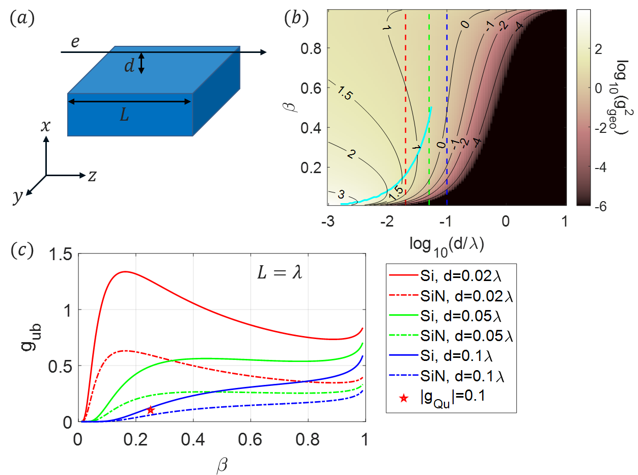
Figure 1: (a) A free electron travels above the surface of a photonic medium at a distance $d$. (b) Log scale $g^{2}_{\text{geo}}$ as a function of $d$ and $\beta$. Only $g_{\text{geo}}^{2}>10^{-6}$ is shown. The cyan curve represents the sub-relativistic peak for each $d$. The red, green and blue dashed lines represent $d=0.02\lambda$, $d=0.05\lambda$, and $d=0.1\lambda$ respectively, where $\lambda=2\pi/k$. (c) The upper bound of $|g_{Qu,m}|$, i.e., $g_{\text{ub}}$, as a function of $\beta$ for silicon (solid curves) or SiN (dash-dot curves) with separation $d=0.02\lambda$, $d=0.05\lambda$, or $d=0.1\lambda$, where $L=\lambda$. The red star represents a numerical example with $|g_{Qu}|=0.1$ (SM Sec. V).

IV Numerical demonstration

In this section, I show numerical examples for the upper bound of $|g_{Qu,m}|$, i.e., $g_{\text{ub}}$ in Eq. 24. Since the scaling with material properties and interaction length are clear in the analytical expression, the numerical demonstration focuses on the last term, referred to as the geometric factor $g^{2}_{\text{geo}}$, which depends on the electron velocity and the separation between the electron beam and the photonic structure ($g^{2}_{\text{geo}}=\int_{R}d^{2}r_{\perp}^{\prime}\big{[}\frac{\alpha_{e}^{4}}{k^{2}}K_{0}^{2}(\alpha_{e}\rho)+\frac{k_{e}^{2}\alpha_{e}^{2}}{k^{2}}K_{1}^{2}(\alpha_{e}\rho)\big{]}$). I study the case where the photonic medium and the free electron can be separated by planes with separation distance $d$ (Fig. 1 (a)) Henke et al. (2021); Yang et al. (2018). $g^{2}_{\text{geo}}$ as a function of $d$ and the normalized electron velocity ($\beta=v/c$) is shown in Fig. 1(b). The color shows $g^{2}_{\text{geo}}$ in log scale if $g^{2}_{\text{geo}}>10^{-6}$.

Figure 1(b) shows that the geometric factor decreases with the separation between the free-electron trajectory and the photonic medium. When the separation is small ($d/\lambda<0.06$, where $\lambda$ is the free-space optical wavelength), the geometric factor is peaked at a sub-relativistic velocity (the cyan curve in Fig. 1(b), besides the divergence as $\beta\rightarrow 1$. To illustrate the influence of the optical medium and free-electron velocity on the upper bound of the coupling coefficient, I plot, in Fig. 1(c), the upper bound ($g_{\text{ub}}$) as a function of $\beta$ for silicon and SiN photonic structures at 3 separation distances: $d=0.02\lambda$, $d=0.05\lambda$, and $d=0.1\lambda$. $g_{\text{ub}}$ for silicon is twice that for SiN, due to its higher permittivity. For deep sub-wavelength separation between the free electron and the optical medium, $g_{\text{ub}}$ has a prominent peak at low electron velocity. For instance, with $d=0.02\lambda$, $L=\lambda$, and a silicon optical medium, $g_{\text{ub}}>1$ at a sub-relativistic velocity $0.1<\beta<0.4$, which is promising to reach strong coupling. Such a sub-relativistic peak in free-electron–light coupling is consistent with previous studies when $d$ is deep sub-wavelength Liebtrau et al. (2021). Although the large $g_{\text{ub}}$ at small $d$ can be diminished with a large free-electron beam size, the analytical upper bound is approximately valid when $d$ is larger than the transverse electron beam size (SM Sec. IV). Furthermore, with a maximal interaction length estimated from the angular spread of a transversely confined free electron Karnieli et al. (2024b), one can find the ultimate upper bound of the quantum coupling coefficient, where a large range of parameters could potentially achieve the strong coupling regime of the free-electron–light interaction (SM Sec. IV). Whether realistic structures can reach this upper bound, especially for slow electrons ($\beta\lesssim 0.3$), relies on extensive search for the optimal design, which is beyond the scope of this study. Nevertheless, as an intuitive example, I numerically study the guided mode in a silicon sub-wavelength grating and find $|g_{Qu}|=0.1$ with $\beta=0.25$ and $L=\lambda$ (red star in Fig. 1(c)), which can reach strong coupling with $L>95\lambda$ (SM Sec. V).

V Conclusion

In conclusion, I study the upper bound for the quantum coupling coefficient describing the interaction between free electrons and photons. I derive the analytical expression of the upper bound when an electron interacts with a general photonic excitation and when the photonic excitation has a discrete spectrum, and I discuss the connections between these two cases. I also provide numerical results to show the dependence of the coupling coefficient upper bound on the free-electron velocity and the separation between the free electron and the optical medium. Our study on the upper bound for the quantum coupling coefficient provides guidance to the choice of system parameters, such as the optical medium, the interaction length, and the free-electron velocity, to reach strong coupling between free electrons and photons.

References

- Barwick et al. (2009) B. Barwick, D. J. Flannigan, and A. H. Zewail, Nature 462, 902 (2009).
- Wang et al. (2020) K. Wang, R. Dahan, M. Shentcis, Y. Kauffmann, A. Ben Hayun, O. Reinhardt, S. Tsesses, and I. Kaminer, Nature 582, 50 (2020).
- Kfir et al. (2020) O. Kfir, H. Lourenço-Martins, G. Storeck, M. Sivis, T. R. Harvey, T. J. Kippenberg, A. Feist, and C. Ropers, Nature 582, 46 (2020).
- Piazza et al. (2015) L. Piazza, T. Lummen, E. Quinonez, Y. Murooka, B. Reed, B. Barwick, and F. Carbone, Nature communications 6, 6407 (2015).
- Kurman et al. (2021) Y. Kurman, R. Dahan, H. H. Sheinfux, K. Wang, M. Yannai, Y. Adiv, O. Reinhardt, L. H. Tizei, S. Y. Woo, J. Li, et al., Science 372, 1181 (2021).
- García de Abajo et al. (2010) F. J. García de Abajo, A. Asenjo-Garcia, and M. Kociak, Nano Letters 10, 1859 (2010).
- Park et al. (2010) S. T. Park, M. Lin, and A. H. Zewail, New Journal of Physics 12, 123028 (2010).
- Feist et al. (2015) A. Feist, K. E. Echternkamp, J. Schauss, S. V. Yalunin, S. Schäfer, and C. Ropers, Nature 521, 200 (2015).
- Pan and Gover (2018) Y. Pan and A. Gover, Journal of Physics Communications 2, 115026 (2018).
- Shiloh et al. (2022) R. Shiloh, T. Chlouba, and P. Hommelhoff, Physical Review Letters 128, 235301 (2022).
- Zhou et al. (2019) J. Zhou, I. Kaminer, and Y. Pan, arXiv preprint arXiv:1908.05740 (2019).
- Pan et al. (2019) Y. Pan, B. Zhang, and A. Gover, Physical Review Letters 122, 183204 (2019).
- Di Giulio et al. (2019) V. Di Giulio, M. Kociak, and F. J. G. de Abajo, Optica 6, 1524 (2019).
- Kfir (2019) O. Kfir, Physical Review Letters 123, 103602 (2019).
- Pan and Gover (2019) Y. Pan and A. Gover, Physical Review A 99, 052107 (2019).
- Remez et al. (2019) R. Remez, A. Karnieli, S. Trajtenberg-Mills, N. Shapira, I. Kaminer, Y. Lereah, and A. Arie, Physical Review Letters 123, 060401 (2019).
- Gruner and Welsch (1996) T. Gruner and D.-G. Welsch, Physical Review A 53, 1818 (1996).
- Dung et al. (1998) H. T. Dung, L. Knöll, and D.-G. Welsch, Physical Review A 57, 3931 (1998).
- Rivera and Kaminer (2020) N. Rivera and I. Kaminer, Nature Reviews Physics 2, 538 (2020).
- Di Giulio and de Abajo (2020) V. Di Giulio and F. J. G. de Abajo, New Journal of Physics 22, 103057 (2020).
- Kfir et al. (2021) O. Kfir, V. Di Giulio, F. J. G. de Abajo, and C. Ropers, Science Advances 7, eabf6380 (2021).
- Huang et al. (2023) G. Huang, N. J. Engelsen, O. Kfir, C. Ropers, and T. J. Kippenberg, PRX Quantum 4, 020351 (2023).
- Ben Hayun et al. (2021) A. Ben Hayun, O. Reinhardt, J. Nemirovsky, A. Karnieli, N. Rivera, and I. Kaminer, Science Advances 7, eabe4270 (2021).
- Feist et al. (2022) A. Feist, G. Huang, G. Arend, Y. Yang, J.-W. Henke, A. S. Raja, F. J. Kappert, R. N. Wang, H. Lourenço-Martins, Z. Qiu, et al., Science 377, 777 (2022).
- Karnieli and Fan (2023) A. Karnieli and S. Fan, Science Advances 9, eadh2425 (2023).
- Dahan et al. (2023) R. Dahan, G. Baranes, A. Gorlach, R. Ruimy, N. Rivera, and I. Kaminer, Physical Review X 13, 031001 (2023).
- Baranes et al. (2023) G. Baranes, S. Even-Haim, R. Ruimy, A. Gorlach, R. Dahan, A. A. Diringer, S. Hacohen-Gourgy, and I. Kaminer, Physical Review Research 5, 043271 (2023).
- Karnieli et al. (2024a) A. Karnieli, S. Tsesses, R. Yu, N. Rivera, A. Arie, I. Kaminer, and S. Fan, PRX Quantum 5, 010339 (2024a).
- Yang et al. (2018) Y. Yang, A. Massuda, C. Roques-Carmes, S. E. Kooi, T. Christensen, S. G. Johnson, J. D. Joannopoulos, O. D. Miller, I. Kaminer, and M. Soljačić, Nature Physics 14, 894 (2018).
- Zhao et al. (2021) Z. Zhao, X.-Q. Sun, and S. Fan, Physical Review Letters 126, 233402 (2021).
- Miller et al. (2016) O. D. Miller, A. G. Polimeridis, M. H. Reid, C. W. Hsu, B. G. DeLacy, J. D. Joannopoulos, M. Soljačić, and S. G. Johnson, Optics express 24, 3329 (2016).
- García de Abajo (2010) F. J. García de Abajo, Reviews of Modern Physics 82, 209 (2010).
- Tsang et al. (2000) L. Tsang, J. A. Kong, and K.-H. Ding, Scattering of electromagnetic waves: theories and applications, Vol. 15 (John Wiley & Sons, 2000).
- Henke et al. (2021) J.-W. Henke, A. S. Raja, A. Feist, G. Huang, G. Arend, Y. Yang, F. J. Kappert, R. N. Wang, M. Möller, J. Pan, et al., Nature 600, 653 (2021).
- Liebtrau et al. (2021) M. Liebtrau, M. Sivis, A. Feist, H. Lourenço-Martins, N. Pazos-Pérez, R. A. Alvarez-Puebla, F. J. G. de Abajo, A. Polman, and C. Ropers, Light: Science & Applications 10, 82 (2021).
- Karnieli et al. (2024b) A. Karnieli, C. Roques-Carmes, N. Rivera, and S. Fan, arXiv preprint arXiv:2403.13071 (2024b).
- Xie et al. (2024) Z. Xie et al., arXiv Submission (2024).