The Rate-Distortion-Perception Trade-off:
The Role of Private Randomness

Abstract

In image compression, with recent advances in generative modeling, the existence of a trade-off between the rate and the perceptual quality (realism) has been brought to light, where the realism is measured by the closeness of the output distribution to the source. It has been shown that randomized codes can be strictly better under a number of formulations. In particular, the role of common randomness has been well studied. We elucidate the role of private randomness in the compression of a memoryless source $X^{n}=(X_{1},...,X_{n})$ under two kinds of realism constraints. The near-perfect realism constraint requires the joint distribution of output symbols $(Y_{1},...,Y_{n})$ to be arbitrarily close the distribution of the source in total variation distance (TVD). The per-symbol near-perfect realism constraint requires that the TVD between the distribution of output symbol $Y_{t}$ and the source distribution be arbitrarily small, uniformly in the index $t.$ We characterize the corresponding asymptotic rate-distortion trade-off and show that encoder private randomness is not useful if the compression rate is lower than the entropy of the source, however limited the resources in terms of common randomness and decoder private randomness may be.

I Introduction

In conventional rate-distortion theory, the objective is to facilitate the reconstruction of a representation, denoted as $Y^{n}\triangleq(Y_{1},...,Y_{n}),$ of a source signal $X^{n}=(X_{1},...,X_{n}),$ while optimizing the proximity between the two, measured by a distortion measure $d(X^{n},Y^{n}).$ The asymptotic regime $n\to\infty$ has been extensively studied, starting with the work of Claude Shannon, who characterized the optimal asymptotic trade-off between rate and distortion, for additive distortion measures, i.e. $d(x^{n},y^{n})=(1/n)\sum_{t=1}^{n}d(x_{t},y_{t}).$ The one-shot scenario $n=1$ has also been studied [1]. Despite the overall success of this theory (e.g. [2, 3]), one notable limitation is the potential for the reconstructed output to manifest qualitatively distinct features from the original source realization. For a memoryless Gaussian source, when optimizing the mean-squared error (MSE) distortion measure, the reconstructed output typically possesses reduced power compared to the source. Consequently, this phenomenon manifests as perceptual blurring in JPEG images at low bit-rates. The concept of distortion measure only serves as a surrogate for the ultimate metric of genuine interest: how the reconstructed output is perceived by the end-user, typically a human observer. In certain scenarios, the latter may exhibit a preference for a reconstruction that registers higher distortion. A noteworthy example is MPEG Advanced Audio Coding (AAC): artificial noise is deliberately introduced into high-frequency bands [3, Sec. 17.4.2], to align the power spectrum of the reconstruction with that of the source.
In conventional rate-distortion theory, it is known that deterministic encoders and decoders are sufficient to achieve the optimal asymptotic rate-distortion performance for a stationary source —as well as the optimal performance for one-shot fixed-length codes [4]. The systematic study of the impact of perceptual quality constraints and randomization on rate and distortion took flight with the works of Li et al. [5, 6, 7, 8] and Saldi et al. [9, 10]. Therein, perceptual quality, or realism, is formalized by requiring the distribution of the reconstruction $Y^{n}$ to be identical to that of the source, or asymptotically arbitrarily close in total variation distance (TVD). See also the work of Delp et al. [11]. Recently, in [12], the authors used generative adversarial networks (GANs) to push the limits of image compression in very low bit-rates by synthesizing image content, such as facades of buildings, using a reference image database. This line of work lead to the introduction [13] —see also [14, 15, 16]— of a relaxed distribution-preservation constraint: the problem is then to characterize the optimal rate for which both distortion constraint $d(X^{n},Y^{n})\leq\Delta,$ and realism constraint $\mathcal{D}(P_{X^{n}},P_{Y^{n}})\leq\lambda$ are met, where $\mathcal{D}$ is a similarity measure, e.g., the TVD or some other divergence. The three-way trade-off between $\Delta,\lambda,$ and the rate, was coined the rate-distortion-perception (RDP) trade-off. We call the above the strong realism constraint, and imperfect strong realism constraint when $\lambda>0.$ The following weaker variant has been recently studied [17]:

$$\forall 1\leq t\leq n,\quad\mathcal{D}(P_{Y_{t}},p_{X})\leq\lambda,$$ (1)

We call this per-symbol realism. Other constraints depending directly on the realizations of the source and the reconstruction have also been considered [10, 17, 18].
The problem of characterizing the role of randomization under different formulations of the realism constraint, such as done in [10], has very recently attracted renewed interest [19, 17] —see also [20, 21] when an additional source is available as side information, and [22, 23] for a successive refinement scenario. The different forms of randomness include private randomness at each of the encoder and decoder, and common randomness, available at both terminals. In the present work, we delve deeper into the role of private randomness. We characterize the five-way trade-off between compression rate, common randomness rate, encoder private randomness rate, decoder private randomness rate and distortion, thereby extending previous results. We consider a memoryless source $X^{n}\sim p_{X}^{\otimes n}$ and the near-perfect strong realism and near-perfect per-symbol realism constraints:

$$\|P_{Y^{n}}-p_{X}^{\otimes n}\|_{TV}\underset{n\to\infty}{\longrightarrow}0$$ (2)

$$\max_{1\leq t\leq n}\|P_{Y_{t}}-p_{X}\|_{TV}\underset{n\to\infty}{\longrightarrow}0,$$ (3)

where $\|\cdot\|_{TV}$ is the TVD. We first introduce a novel soft covering result regarding the private randomness of stochastic compressors. Then, we show that whether encoder private randomness is available does not impact the optimal asymptotic trade-off between rate and distortion. This holds whatever the resources in terms of common randomness and decoder private randomness are, as long as the compression rate is less than the entropy of the source. This implies that in the absence of common randomness, it is not useful, in the limit of large blocklength $n,$ that the encoder include in its message a seed for a pseudo-random number generator. In other words, the only useful form of shared randomness is a common randomness available without communication.
The RDP trade-off has strong ties to the channel simulation problem, a.k.a. reverse channel coding, a.k.a. channel synthesis, which can be stated [24] as that of finding the optimal rate such that

$$\|P_{X^{n},Y^{n}}-p_{X,Y}^{\otimes n}\|_{TV}\underset{n\to\infty}{\longrightarrow}0,$$

for some target $p_{X,Y}.$ This problem has recently had successful applications in neural network based compression [25, 26] and Federated Learning [27, 28]. Moreover, a channel simulation scheme was used to prove the first coding theorem [29] regarding the RDP trade-off with imperfect realism. In the present work, we use proof techniques from the channel simulation literature: our proofs track those of [24], and we use several of the soft covering lemma variants therein. The paper is organized as follows. We give the problem formulation in Section II, and introduce a key lemma in Section III. We present all our other results in Section IV, and provide a partial proof in Section V. The rest of the proofs is provided in the appendices.

II Problem formulation

II-A Notation

Calligraphic letters such as $\mathcal{X}$ denote sets, except in $p^{\mathcal{U}}_{\mathcal{J}},$ which denotes the uniform distribution over alphabet $\mathcal{J}.$ Random variables are denoted using upper case letters such as $X,$ and their realizations using lower case letters such as $x.$ For a distribution $P,$ the expression $P_{X}$ denotes the marginal of variable $X,$ while $P(x)$ denotes the probability of the event $X{=}x.$ Similarly, $P_{X|Y{=}y}$ denotes a distribution over $\mathcal{X},$ and $P_{X|Y{=}y}(x)$ a real number. We denote by $\mathbf{1}_{X{=}x_{0}}$ the distribution such that the events $X{=}x_{0}$ and $X{\neq}x_{0}$ have probabilities $1$ and $0.$ We denote by $[a]$ the set $\{1,...,\lfloor a\rfloor\},$ and by $x^{n}$ the finite sequence $(x_{1},...,x_{n}).$ The TVD between distributions $p$ and $q$ on a space $(\mathcal{X},\mathcal{B})$ is defined by

$$\|p-q\|_{TV}:=\sup_{B\in\mathcal{B}}|p(B)-q(B)|.$$

The closure of a set $\mathcal{A}$ is denoted by $\overline{\mathcal{A}}.$ We use the definitions in [30] for the entropy $H(X)$ and mutual information $I(X;Y)$ for random variables $X$ and $Y$ taking values in some Polish spaces. This includes discrete spaces and real vector spaces. We always endow a Polish alphabet with the corresponding Borel $\sigma$-algebra. It contains all singletons. All conditional probability kernels we consider are regular. We define $\overline{\mathbb{R}}_{\geq 0}{:=}\mathbb{R}_{\geq 0}{\cup}\{\infty\}$ and use the convention $\infty{\geq}\infty.$ The notation $\overset{\mathcal{P}}{\rightarrow}$ stands for convergence in probability. For a finite alphabet $\mathcal{X},$ $\mathbb{P}^{\text{emp}}_{\mathcal{X}}(x^{n})$ is the empirical distribution of $x^{n}{\in}\mathcal{X}^{n}.$ Given a distribution $P_{X^{n}}$ on $\mathcal{X}^{n},$ we denote by $\hat{P}_{\mathcal{X}}[X^{n}]$ the average empirical distribution of random string $X^{n},$ i.e., the distribution on $\mathcal{X}$ defined by: for any measurable $A{\subseteq}\mathcal{X},$

II-B Definitions

Definition 1

Given a space $\mathcal{X},$ a distortion measure is a measurable function $d:\mathcal{X}^{2}{\to}[0,\infty)$ extending to sequences as

$$d(x^{n},y^{n})=\tfrac{1}{n}\scalebox{0.95}{$\sum_{t=1}^{n}$}d(x_{t},y_{t}).$$

As shown in Figure 1, we consider common randomness and decoder private randomness available at rates $R_{c}$ and $R_{d},$ respectively, which may be infinite. We consider both fixed-length and variable-length codes. Either the encoder private randomness is unconstrained, or it is completely unavailable.

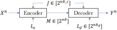
Figure 1: The system model.

Definition 2

Given a space $\mathcal{X}$ and a triplet $(R,R_{c},R_{d})\in\mathbb{R}_{\geq 0}\times\overline{\mathbb{R}}_{\geq 0}^{2},$ an $(n,R,R_{c},R_{d})$ variable-length code is a tuple $(p_{J},p_{L_{e}},p_{L_{d}},F^{(n)},G^{(n)})$ consisting of distributions $p_{J},p_{L_{e}},p_{L_{d}}$ on some Polish spaces, a deterministic encoder

$$F^{(n)}:(X^{n},J,L_{e})\mapsto M$$ (4)

with some Polish output space, and a deterministic decoder

$$G^{(n)}:(M,J,L_{d})\mapsto Y^{n}\in\mathcal{X}^{n},\quad\text{satisfying}$$ (5)

$$R\geq\tfrac{1}{n}H(M),\quad R_{c}\geq\tfrac{1}{n}H(J),\quad R_{d}\geq\tfrac{1}{n}H(L_{d}).$$

Given a distribution $p_{X}$ on $\mathcal{X},$ the distribution induced by the code is given by

$$P_{X^{n},J,L_{e},M,L_{d},Y^{n}} := p_{X}^{\otimes n}\cdot p_{J}\cdot p_{L_{e}}\cdot p_{L_{d}}\cdot\mathbf{1}_{M{=}F^{(n)}(x^{n},j,l_{e})}$$

$$\cdot \mathbf{1}_{Y^{n}{=}G^{(n)}(m,j,l_{d})}.$$

Note that if any of $R,R_{c},R_{d}$ is null, then the corresponding random variable ($M$ or $J$ or $L_{d}$) is constant $P$-almost surely —see e.g. the discussion above [30, Lemma 7.18]. Given a triplet $(R,R_{c},R_{d})\in\mathbb{R}_{\geq 0}^{3},$ an $(n,R,R_{c},R_{d})$ fixed-length code is an variable-length code such that

$$M\in[2^{nR}]\text{ a.s.,}\quad p_{J}\equiv p^{\mathcal{U}}_{[2^{nR_{c}}]},\quad p_{L_{d}}\equiv p^{\mathcal{U}}_{[2^{nR_{d}}]}.$$

No constraint (alphabet, distribution, rate) is imposed on the encoder private randomness of a fixed-length (resp. variable-length) code. Similarly, we define an $(n,R,R_{c},\infty)$ fixed-length code as a variable-length code with $M\in[2^{nR}]\text{ a.s.}$ and $p_{J}\equiv p^{\mathcal{U}}_{[2^{nR_{c}}]}.$ An $(n,R,R_{c},R_{d})$ fixed-length (resp. variable-length) code with non-privately randomized encoding is an $(n,R,R_{c},R_{d})$ fixed-length (resp. variable-length) code for which $L_{e}$ is constant $P$-almost surely.

Definition 3

Consider a space $\mathcal{X},$ a distribution $p_{X}$ on $\mathcal{X},$ and a distortion measure $d.$ A tuple $(R,R_{c},R_{d},\Delta)\in\mathbb{R}_{\geq 0}\times\overline{\mathbb{R}}_{\geq 0}^{3}$ is said to be achievable with near-perfect realism with fixed-length (resp. variable-length) codes with privately randomized (resp. non-privately randomized) encoding if there exists a sequence of $(n,R,R_{c},R_{d})$ fixed-length (resp. variable-length) codes with privately randomized (resp. non-privately randomized) encoding with induced distributions $\{P^{(n)}\}_{n}$ such that

(6)

(7)

For each of the above notions of achievability, we introduce the corresponding notion of achievability with per-symbol near-perfect realism, defined by replacing (7) by

(8)

The similar notions of achievability with perfect realism or perfect per-symbol realism are defined by replacing (7) by:

(9)

(10)

III A soft covering lemma for randomized compressors

III-A Statement

Proposition 4

Consider a finite input alphabet $\mathcal{X},$ a distribution $p_{X}$ on $\mathcal{X},$ non-negative reals $R,R_{c}$ and a sequence $\{F^{(n)}\}_{n\geq 1}$ of encoders corresponding to a sequence of $(n,R,R_{c},\infty)$ fixed-length codes. The $n$-th induced distribution is denoted $P^{(n)}.$ If $R<H(X),$ then for any finite alphabet $\mathcal{V}$ and any sequence of deterministic mappings $\mathbf{v}^{(n)}:[2^{nR}]\times[2^{nR_{c}}]\to\mathcal{V}^{n},$ there exists a sequence of deterministic maps

(11)

$$\tilde{P}^{(n)}_{X^{n},J,M}:=p_{X}^{\otimes n}\cdot p^{\mathcal{U}}_{[2^{nR_{c}}]}\cdot\mathbf{1}_{M=f^{(n)}(X^{n},J)}.$$

The result follows rather directly from applying the soft covering lemma with a sequence of general sources and channels [24, Corollary VII.3]. We provide a proof in Appendix B.

Remark 5

Consider the setting of Proposition 4 and let $\{G^{(n)}\}_{n\geq 1}$ be the sequence of decoders in the initial codes. Assume that there exists a finite alphabet $\mathcal{V},$ a conditional probability $P_{Y|V}$ from $\mathcal{V}$ to $\mathcal{X},$ and a sequence $\{\mathbf{v}^{(n)}\}_{n\geq 1}$ of deterministic maps with $\mathbf{v}^{(n)}:[2^{nR}]\times[2^{nR_{c}}]\to\mathcal{V}^{n},$ such that for any $(m,j)$ we have

(12)

Then, —e.g. Lemma 16, Appendix A—, sequence $\{f^{(n)}\}_{n{\geq}1}$ of Proposition 4 corresponding to $\{\mathbf{v}^{(n)}\}_{n\geq 1}$ satisfies

$$\scalebox{0.85}{$\big{\|}\hat{\tilde{P}}^{(n)}_{\mathcal{X}^{2}\times\mathcal{V}}$}\scalebox{0.8}{$[X^{n},Y^{n},\mathbf{v}^{(n)}(M,J)]$}-\scalebox{0.85}{$\hat{P}^{(n)}_{\mathcal{X}^{2}\times\mathcal{V}}$}\scalebox{0.8}{$[X^{n},Y^{n},\mathbf{v}^{(n)}(M,J)]$}\scalebox{0.8}{$\big{\|}_{TV}\underset{n\to\infty}{\longrightarrow}0$}$$

(13)

IV The rate-distortion-perception trade-off with near-perfect realism

IV-A The role of encoder private randomness for finite source alphabets

We have the following characterization, which is an extension of [10, Theorems 1 & 5]. The achievability is proved in Section V, and the converse in Appendix C.

Theorem 6

Consider a finite source alphabet $\mathcal{X},$ a distribution $p_{X}$ on $\mathcal{X}$ and a distortion measure $d.$ Define the region $\mathcal{S}_{D}$ of $[0,H(X))\times\overline{\mathbb{R}}_{\geq 0}^{3}$ as

$$\left\{\begin{array}[]{rcl}\scalebox{0.9}{$(R,R_{c},R_{d},\Delta)$}&:&\scalebox{0.9}{$\exists\ p_{X,V,Y}\in\mathcal{D}_{D},$}\\ \scalebox{0.9}{$R$}&\geq&\scalebox{0.9}{$I_{p}(X;V)$}\\ \scalebox{0.9}{$R+R_{c}$}&\geq&\scalebox{0.9}{$I_{p}(Y;V)$}\\ \scalebox{0.9}{$R_{d}$}&\geq&\scalebox{0.9}{$H_{p}(Y|V)$}\\ \scalebox{0.9}{$\Delta$}&\geq&\scalebox{0.9}{$\mathbb{E}_{p}[d(X,Y)]$}\end{array}\right\},$$ (19)

with $\mathcal{D}_{D}$ defined as

$$\left\{\begin{array}[]{rcl}&p_{X,V,Y}:\scalebox{0.9}{$X\sim$ }p_{X},\ p_{Y}\equiv p_{X}&\\ &X-V-Y&\\ &|\mathcal{V}|\leq|\mathcal{X}|^{2}+1&\end{array}\right\}.$$ (23)

Denote by $\mathcal{A}^{(f)}_{D}$ the set of $(R,R_{c},R_{d},\Delta)\in[0,H(X))\times\mathbb{R}_{\geq 0}^{3}$ achievable with near-perfect realism with fixed-length codes and by $\mathcal{A}^{(u)}_{D}$ the set of tuples $(R,R_{c},R_{d},\Delta)\in[0,H(X))\times\overline{\mathbb{R}}_{\geq 0}^{3}$ achievable with near-perfect realism with variable-length codes. Denote by $\mathcal{A}^{(f,*)}_{D}$ the set of tuples $(R,R_{c},R_{d},\Delta)\in[0,H(X))\times\mathbb{R}_{\geq 0}^{3}$ achievable with near-perfect realism with non-privately randomized encoding and by $\mathcal{A}^{(u,*)}_{D}$ the set of tuples $(R,R_{c},R_{d},\Delta)\in[0,H(X))\times\overline{\mathbb{R}}_{\geq 0}^{3}$ achievable with near-perfect realism with variable-length codes and non-privately randomized encoding. Then,

1. the aforementioned sets have identical closures in $\overline{\mathbb{R}}_{\geq 0}^{4}:$

   $$\overline{\mathcal{A}^{(f)}_{D}}=\overline{\mathcal{A}^{(u)}_{D}}=\overline{\mathcal{A}^{(f,*)}_{D}}=\overline{\mathcal{A}^{(u,*)}_{D}}=\overline{S_{D}}.$$ (24)

2. the same holds if each notion of achievability is replaced by the corresponding achievability with no common randomness $(R_{c}=0)$ and $\mathcal{S}_{D}$ is replaced by its intersection with the hyperplane $R_{c}=0.$

3. the same holds if each notion of achievability is replaced by the corresponding achievability with no decoder private randomness $(R_{d}=0)$ and $\mathcal{S}_{D}$ is replaced by its intersection with the hyperplane $R_{d}=0.$

Consequently, for lossy compression $(R{<}H(X))$ with a near-perfect realism constraint, encoder private randomness is not useful whatever the available resources in terms of common randomness and decoder private randomness are. In particular, this holds even if the latter two sources of randomness are not rate-limited or not discrete. It is unclear whether encoder private randomness may be useful when the compression rate $R$ is greater than or equal to the entropy of the source.

IV-B An extension to sources with infinite entropy

Following [19], we use the following assumption in order to handle general alphabets.

Definition 7

[19] Given a space $\mathcal{X},$ a probability distribution $p$ on $\mathcal{X}$ and a distortion measure $d,$ we say that $(d,p)$ is uniformly integrable if and only if

$$\forall\varepsilon>0,\exists\tau>0,\quad\sup_{\mathbb{P}_{X,Y,\xi}}\mathbb{E}[d(X,Y)\cdot\xi]\leq\varepsilon,$$

where the supremum is taken over all distributions $\mathbb{P}_{X,Y,\xi}$ on $\mathcal{X}^{2}\times\{0,1\}$ satisfying $\mathbb{P}_{X}\equiv\mathbb{P}_{Y}\equiv p$ and $\mathbb{P}(\{\xi=1\})\leq\tau.$

The property of Definition 7 is satisfied if $\mathcal{X}$ is finite and $d$ does not take infinite values. It is also satisfied if $\mathcal{X}\subseteq\mathbb{R},$ $d$ is the MSE distortion measure, and $p_{X}$ has a finite second moment, as proved in [17, Appendix E]. Our approach for turning a privately randomized encoder into a non-privately randomized one requires to work with finite alphabets. To that end, we introduce the following notion, which involves a standard formalism for the notion of arbitrarily fine quantization. A quantizer on a measurable space $\mathcal{X}$ is any measurable finite-valued map from $\mathcal{X}$ onto itself.

Definition 8

Consider a source alphabet $\mathcal{X},$ a $\sigma$-algebra $\mathcal{B}$ of subsets of $\mathcal{X},$ a probability distribution $p$ on $(\mathcal{X},\mathcal{B})$ and a distortion measure $d.$ We say that $(d,p)$ is quantizable if the following holds: there exists a sequence $\{\kappa^{(\ell)}\}_{\ell\in\mathbb{N}}$ of quantizers of $\mathcal{X}$ such that the corresponding partitions asymptotically generate $\mathcal{B},$ and for any $\tau,\varepsilon>0,$

$$\exists B_{\tau}\in\mathcal{B},\quad p(\mathcal{X}\setminus B_{\tau})\leq\tau,$$ (25)

and there exists $L_{\varepsilon,\tau}$ such that for any $\ell\geq L_{\varepsilon,\tau},$

$$\forall(x,y)\in B_{\tau}^{2},\quad\big{|}d(x,y)-d\big{(}\kappa^{(\ell)}(x),\kappa^{(\ell)}(y)\big{)}\big{|}\leq\varepsilon,$$ (26)

$$\forall(x,y)\in\mathcal{X}^{2}\setminus B_{\tau}^{2},\quad d\big{(}\kappa^{(\ell)}(x),\kappa^{(\ell)}(y)\big{)}\leq d(x,y)+\varepsilon.$$ (27)

This property is satisfied if $\mathcal{X}$ is finite, and we have

Claim 9

If $\mathcal{X}$ is a finite-dimensional real vector space and $d$ denotes the Euclidean distance, then for any distribution $p$ on $\mathcal{X}$ and any $s>0,$ tuple $(d^{s},p)$ is quantizable.

We provide a proof in Appendix G-C. We have the following characterization, which is an extension of [10, Theorem 1] and [19, Theorem 2]. The proof is provided in Appendix E.

Theorem 10

Consider a Polish source alphabet $\mathcal{X},$ a distribution $p_{X}$ on $\mathcal{X}$ having infinite entropy, and a distortion measure $d$ such that $(d,p_{X})$ is uniformly integrable and quantizable. Define the region $\mathcal{S}_{G}$ as

$$\left\{\begin{array}[]{rcl}\scalebox{0.9}{$(R,R_{c},\Delta)\in\mathbb{R}_{\geq 0}^{3}$}&:&\scalebox{0.9}{$\exists\ p_{X,V,Y}\in\mathcal{D}_{G}\text{ s.t. }$}\\ \scalebox{0.9}{$R$}&\geq&\scalebox{0.9}{$I_{p}(X;V)$}\\ \scalebox{0.9}{$R+R_{c}$}&\geq&\scalebox{0.9}{$I_{p}(Y;V)$}\\ \scalebox{0.9}{$\Delta$}&\geq&\scalebox{0.9}{$\mathbb{E}_{p}[d(X,Y)]$}\end{array}\right\},$$ (32)

with $\mathcal{D}_{G}$ defined as

$$\left\{\begin{array}[]{rcl}&p_{X,V,Y}:\scalebox{0.9}{$X\sim$ }p_{X},\ p_{Y}\equiv p_{X}&\\ &X-V-Y&\end{array}\right\},$$ (35)

where the alphabet of $V$ is constrained to be finite. Denote by $\mathcal{A}_{G}$ the set of triplets $(R,R_{c},\Delta)\in\mathbb{R}_{\geq 0}^{3}$ such that $(R,R_{c},\infty,\Delta)$ is achievable with near-perfect realism with fixed-length codes, and by $\mathcal{A}^{(f,*)}_{G}$ the set of triplets $(R,R_{c},\Delta)\in\mathbb{R}_{\geq 0}^{3}$ such that $(R,R_{c},\infty,\Delta)$ is achievable with near-perfect realism with fixed-length codes and non-privately randomized encoding. Then,

1. the aforementioned sets have identical closures in $\mathbb{R}_{\geq 0}^{3}:$

   $$\overline{\mathcal{A}^{(f)}_{G}}=\overline{\mathcal{A}^{(f,*)}_{G}}=\overline{S_{G}}.$$ (36)

2. the same holds if each notion of achievability is replaced by the corresponding achievability with no common randomness $(R_{c}=0)$ and $\mathcal{S}_{G}$ is replaced by its intersection with the hyperplane $R_{c}=0.$

The assumption of unlimited decoder private randomness is not very restrictive as far as the study of encoder private randomness is concerned. Indeed, for most general alphabets of interest, the total variation distance between a distribution having finite entropy and a distribution having infinite entropy is equal to $1.$ Hence, if the source distribution has infinite entropy, then achievability with near-perfect realism requires either $R_{d}$ or $R_{c}$ to be infinite (assuming $R$ is finite). Moreover, the case of unconstrained common randomness is trivial: there is no use for local randomness, since unlimited randomness can be extracted from the common randomness. We conjecture that the assumptions of finite-valued auxiliary variable $V$ and fixed-length codes are not restrictive.

IV-C Per-symbol realism

The following theorem is an extension of [17, Theorem 4], which states that under a perfect per-symbol realism constraint, whether common randomness is available does not impact the optimal asymptotic trade-off between rate and distortion. We find that the same can be said of encoder private randomness, if only near-perfect per-symbol realism is required.

Theorem 11

Theorems 6 and 10 also hold if achievability with near-perfect realism is replaced by achievability with per-symbol near-perfect realism, and each lower bound on $R+R_{c}$ is removed in $\mathcal{S}_{D}$ and $\mathcal{S}_{G}.$

A proof is provided in Appendix F. Our result also complements [17, Theorem 2], which states that under the per-symbol realism constraint (1), if $\lambda>0,$ then fully determinitic codes are sufficient to achieve the optimal asymptotic trade-off.

V Achievability proof for Theorem 6

V-A Modifying a standard code construction

A rather straightforward adaptation of the proof of [19, Theorem 2] yields the following result.

Proposition 12

Consider finite alphabets $\mathcal{X},\mathcal{V},$ a distortion measure $d$ on $\mathcal{X}^{2},$ a triplet $(R,R_{c},\Delta)\in\mathbb{R}_{\geq 0}^{3},$ and a distribution $p_{X,Y,V}$ on $\mathcal{X}^{2}\times\mathcal{V}.$ Assume that $p\in\mathcal{D}_{D}$ and

Then, there exists a sequence $\{\varepsilon_{n}\}_{n\geq 1}$ of positive reals and a sequence of $(n,R+\varepsilon_{n},R_{c},\infty)$ fixed-length codes inducing distributions $\{P^{(n)}_{X^{n},J,M,Y^{n}}\}_{n\geq 1}$ such that $\varepsilon_{n}\underset{n\to\infty}{\rightarrow}0$ and

(37)

(38)

(39)

(40)

for some sequence of deterministic functions $v^{(n)}:[2^{n(R+\varepsilon)}]{\times}[2^{nR_{c}}]\to\mathcal{V}^{n}.$

See Appendix G-A for a proof. As a direct consequence of Proposition 4 and Remark 5, we can state the following.

Proposition 13

For $R<H(X),$ Proposition 12 holds with $P^{(n)}$ induced by a $(n,R+\varepsilon_{n},R_{c},\infty)$ fixed-length code with non-privately randomized encoding, for large enough $n.$

V-B Achievability of Theorem 6

By definition, for each of the three statements of Theorem 6, we know that $\mathcal{A}^{(f)}_{D},\mathcal{A}^{(u)}_{D},\mathcal{A}^{(u,*)}_{D}$ contain $\mathcal{A}^{(f,*)}_{D}.$ In this section, we consider the (more general) setting of the first statement and prove that $\mathcal{S}_{D}{\subseteq}\overline{\mathcal{A}^{(f,*)}_{D}}.$ Throughout the section, we explain how our proof implies that the same holds in the respective settings of the two other statements. Let $(R,R_{c},R_{d},\Delta)$ be a tuple in $\mathcal{S}_{D}$ and $p_{X,V,Y}$ be a corresponding distribution in $\mathcal{D}_{D}.$ If $R_{c}=\infty,$ we replace it by $H(X),$ if $R_{d}=\infty,$ we replace it with $H(Y|X),$ and if $\Delta=\infty,$ we replace it with $\max(d),$ which exists since $\mathcal{X}$ is finite and $d$ is assumed to only take finite values (Definition 1). Then, $(R,R_{c},R_{d},\Delta)\in[0,H(X))\times\mathbb{R}_{\geq 0}^{3},$ and we can apply Proposition 13. Hereafter, we use the notation of Proposition 13. If $R_{d}=0,$ then $H_{p}(Y|V)=0,$ thus from (39), for any $n\in\mathbb{N},$ $P^{(n)}$ is the distribution induced by a $(n,R+\varepsilon_{n},R_{c},0)$ fixed-length code. Hence, under the setting of the third statement of Theorem 6, we have $\mathcal{S}_{D}{\subseteq}\overline{\mathcal{A}^{(f,*)}_{D}},$ which concludes the proof regarding that setting. Moving to the case $R_{d}>0,$ we can use the same argument as in [24, Appendix 2] and reach the following claim —see Appendix G-B for a proof.

Claim 14

From the local channel synthesis lemma [24, Corollary VII.6], (39) and (40), for any $\gamma>0$ and any $n\in\mathbb{N},$ there exists a mapping $\tilde{P}_{Y^{n}|V^{n}}$ with a fixed-length private randomness of rate $H_{p}(Y|V)+\gamma$ such that

Hence, from Lemmas 15 and 18, and since $d$ is bounded, replacing $P^{(n)}_{Y^{n}|V^{n}}$ by $\tilde{P}_{Y^{n}|V^{n}}$ for every $n$ preserves (37) and (38), and results in a $(n,R+\varepsilon_{n},R_{c},R_{d}+\gamma)$ fixed-length code. This holds for every $\gamma>0.$ Since the common randomness rate used is precisely $R_{c},$ both when $R_{d}=0$ and when $R_{d}>0,$ this shows that we have $\mathcal{S}_{D}\in\overline{A^{(f,*)}_{D}}$ in both the settings of the first and second statements of Theorem 6, which concludes the proof.

VI Conclusion

We have studied the role of private randomness in the rate-distortion-perception trade-off with near-perfect realism and near-perfect per-symbol realism constraints, in the classical infinite blocklength scenario. Our work complements previous results on the key role of randomization in these settings. We have characterized the corresponding rate-distortion-perception trade-offs under different situations in terms of the amount of common and private randomness available. Our results show that encoder private randomness is not useful when the compression rate is lower than the entropy of the source. In particular, in that case, if no common randomness is available, it is not useful to send randomness from the encoder. A similar phenomenon was conjectured [24] to hold for the channel synthesis problem, but this has not yet been proved. The role of encoder private randomness in the finite-blocklength compression setting merits further investigation.

Appendix A Some lemmas on the total variation distance

Lemma 15

[24, Lemma V.1] Let $\Pi$ and $\Gamma$ be two distributions on an alphabet $\mathcal{W}\times\mathcal{L}.$ Then

$$\|\Pi_{W}-\Gamma_{W}\|_{TV}\leq\|\Pi_{W,L}-\Gamma_{W,L}\|_{TV}.$$

Lemma 16

[24, Lemma V.2] Let $\Pi$ and $\Gamma$ be two distributions on an alphabet $\mathcal{W}\times\mathcal{L}.$ Then when using the same channel $\Pi_{L|W}$ we have

$$\|\Pi_{W}\Pi_{L|W}-\Gamma_{W}\Pi_{L|W}\|_{TV}=\|\Pi_{W}-\Gamma_{W}\|_{TV}.$$

Lemma 17

Let $\Pi$ be two distributions on the product of two Polish spaces $\mathcal{W}$ and $\mathcal{L},$ and let $\Pi_{L|W},\Gamma_{L|W}$ be two channels. Then, we have

$$\|\Pi_{W}\Pi_{L|W}-\Pi_{W}\Gamma_{L|W}\|_{TV}=\mathbb{E}_{\Pi_{W}}\big{[}\|\Pi_{L|W}-\Gamma_{L|W}\|_{TV}\big{]}.$$

Lemma 18

Let $\Pi$ and $\Gamma$ be two distributions on a set $\mathcal{W},$ and $f:\mathcal{W}\to\mathbb{R}$ be a bounded function. Then,

$$|\ \mathbb{E}_{\Pi}[f]-\mathbb{E}_{\Gamma}[f]\ |\leq 2\max|f|\cdot\|\Pi-\Gamma\|_{TV}.$$

Appendix B Proof of Proposition 4

We use the soft covering lemma with a sequence of general sources and channels [24, Corollary VII.3], which we state for completeness. For any distribution $\Phi_{V,W},$ we use the notation

$$i_{\Phi}(v;w)=\log(\Phi(v,w)/\Phi(v)\Phi(w))$$

$$i_{\Phi}(w)=-\log(\Phi(w)).$$

Lemma 19

[24, Corollary VII.3] Let $\{\mathcal{U}^{(n)},\mathcal{V}^{(n)},\mathcal{W}^{(n)}\}_{n\geq 1}$ be a sequence of finite alphabets and $\{\Phi_{U^{(n)},V^{(n)},W^{(n)}}\}_{n{\geq}1}$ be a sequence of distributions, the $n$-th being on $\mathcal{U}^{(n)}{\times}\mathcal{V}^{(n)}{\times}\mathcal{W}^{(n)}$. For every $n{\geq}1,$ and every $w^{(n)}{\in}\mathcal{W}^{(n)},$ let $u^{(n)}(w^{(n)})$ be a random variable with distribution $\Phi_{U^{(n)}|W^{(n)}=w^{(n)}}.$ Denote the family $\{u^{(n)}(w^{(n)})\}_{w^{(n)}{\in}\mathcal{W}^{(n)}}$ by $\mathcal{B}^{(n)}.$ For every $n{\geq}1,$ define

Assume that

(41)

Then, we have

$$\mathbb{E}_{\mathcal{B}^{(n)}}[\|\tilde{\Phi}_{V^{(n)}}-\Phi_{V^{(n)}}\|_{TV}]\underset{n\to\infty}{\longrightarrow}0.$$ (42)

For every $n{\geq}1$ let $M{=}\psi^{(n)}(X^{n},J,U)$ be a functional representation of $F^{(n)}.$ Take $\Phi_{W^{(n)},U^{(n)},V^{(n)}}$ corresponding to $P^{(n)}$ with $W^{(n)}{=}(X^{n},J),$ $U^{(n)}{=}U,$ and $V^{(n)}{=}(M,J,\mathbb{P}^{\text{emp}}_{X^{n},\mathbf{v}^{(n)}(M,J)}).$

Proving (41)
Since $V^{(n)}$ is a deterministic function of $(W^{(n)},U^{(n)}),$ it can be easily checked that $1/\Phi_{V^{(n)}}$ is a density for $\Phi_{W^{(n)},U^{(n)},V^{(n)}}$ with respect to $\Phi_{W^{(n)},U^{(n)}}\cdot\Phi_{V^{(n)}}.$ Consider $\varepsilon_{1},\varepsilon_{2}\in(0,H(X){-}R)$ such that $\varepsilon_{1}+\varepsilon_{2}<H(X){-}R.$

$$\IEEEeqnarraymulticol{3}{l}{P^{(n)}\big{(}i_{P^{(n)}}(M,J,\mathbb{P}^{\text{emp}}_{X^{n},\mathbf{v}^{(n)}(M,J)})\geq n(R+R_{c}+\varepsilon_{1})\big{)}}$$

$$=\ P^{(n)}\big{(}P^{(n)}(M,J,\mathbb{P}^{\text{emp}}_{X^{n},\mathbf{v}^{(n)}(M,J)})\leq 2^{-n(R+R_{c}+\varepsilon_{1})}\big{)}$$

$$\leq\ \lfloor 2^{nR}\rfloor\cdot\lfloor 2^{nR_{c}}\rfloor\cdot n^{|\mathcal{X}||\mathcal{V}|}\cdot 2^{-n(R+R_{c}+\varepsilon_{1})}\underset{n\to\infty}{\longrightarrow}0.\qquad\quad$$

Since $J$ is uniformly distributed and independent of $X^{n},$ and $P^{(n)}_{X^{n}}\equiv p_{X}^{\otimes n},$ then for any $(x^{n},j)$ we have $i_{P^{(n)}}(x^{n},j)=i_{p_{X}^{\otimes n}}(x^{n})+\log(\lfloor 2^{nR_{c}}\rfloor).$ From the law of large numbers:

$$P^{(n)}(i_{P^{(n)}}(X^{n},J)\leq n(H(X)+R_{c}-\varepsilon_{2}))\underset{n\to\infty}{\longrightarrow}0.$$

When both the above events do not hold, we have

$$i_{P}(M,J)-i_{P}(X^{n},J)\leq-n(H(X)-R-\varepsilon_{1}-\varepsilon_{2}).$$

Hence, (41) holds.

Conclusion
For each $n{\geq}1,$ choose a realization of $\mathcal{B}^{(n)}$ giving a total variation distance below average, which defines a deterministic

$$f^{(n)}:(x^{n},j)\mapsto\psi^{(n)}(x^{n},j,u^{(n)}(x^{n},j))\in[2^{nR}].$$ (43)

Moreover, for every $n{\geq}1,$ $\tilde{\Phi}^{(n)}$ defines the same distribution of inputs $(X^{n},J)$ as do the distributions $\tilde{P}^{(n)}$ of Proposition 4. We conclude using Lemma 15, and the fact that the empirical distribution is bounded and the average empirical distribution is its expectation, because $\mathcal{X}\times\mathcal{V}$ is finite.

Appendix C Converse of Theorem 6

By definition, for each of the three statements of Theorem 6, we know that $\mathcal{A}^{(f)}_{D},\mathcal{A}^{(f,*)}_{D},\mathcal{A}^{(u,*)}_{D}$ are included in $\mathcal{A}^{(u)}_{D}.$ Therefore, we only prove that $\mathcal{A}^{(u)}_{D}{\subseteq}\mathcal{S}_{D},$ in the setting of the first statement, and this also implies the same relation in the respective settings of the two other statements. This proof closely tracks that of [24, Section VI] and the end of [24, Appendix 2]. Let $(R,R_{c},R_{d},\Delta)\in[0,H(X))\times\overline{\mathbb{R}}_{\geq 0}^{3}$ be achievable with near-perfect realism with variable-length codes. Fix $\varepsilon$ $\in$ $(0,1/4).$ Then, for $n$ large enough, there exists a $(n,R,R_{c},R_{d})$ code inducing a joint distribution $P_{X^{n},J,M,Y^{n}}$ such that

$$\mathbb{E}_{P}[d(X^{n},Y^{n})]\,{\leq}\,\Delta\,{+}\,\varepsilon,\ \|P_{Y^{n}}{-}p_{X}^{\otimes n}\|_{TV}\leq\varepsilon$$

Following the proof of [19, Theorem 2] and [24, Section VI & Appendix 2], we have the following claim.

Claim 20

By introducing a random index uniformly distributed on $[n],$ one can construct a distribution $P^{(\varepsilon)}_{X,Y,V}$ on $\mathcal{X}^{2}\times\mathcal{V}$ satisfying $X{-}V{-}Y,\ \|P_{Y}{-}p_{X}\|_{TV}{\leq}\varepsilon,$ and rate bounds

for some deterministic function $g$ such that $g(\varepsilon){\to}0$ as $\varepsilon{\to}0.$

See Appendix D for a proof. We can change $V$ so that $|\mathcal{V}|{\leq}|\mathcal{X}|^{2}{+}1$ while preserving $P^{(\varepsilon)}_{X,Y},$ the Markov chain $X{-}V{-}Y,$ and quantities $I(X;V),I(Y;V)$ (and thus $H(Y|V)$).

This follows from the proof of [24, Lemma VI.1]. We then conclude with the same argument as in [24, Section VI], as follows. Consider a vanishing sequence $\{\varepsilon_{n}\}_{n\geq 1}$ in $(0,1/4).$ Owing to the cardinality bound, all probabilities $P^{(\varepsilon_{n})}$ can be considered as points in the compact standard simplex of $\mathbb{R}^{2|\mathcal{X}|{+}|\mathcal{X}|^{2}{+}1}.$ Hence, a sub-sequence converges towards some probability $P^{*}_{X,V,Y}$ in the latter. This distribution satisfies the Markov chain constraint and $P^{*}_{X}{\equiv}p_{X}{\equiv}P^{*}_{Y}.$ Hence, $P^{*}{\in}\mathcal{D}_{D}.$ Moreover, since $R{<}H(X)$ and $g(\varepsilon_{n}){\to}0$ as $n{\to}\infty,$ and from the rate lower bounds in Claim 20, we have $(R,R_{c},R_{d},\Delta){\in}\mathcal{S}_{D},$ which concludes the converse proof.

Appendix D Rate lower bounds in the converse proof

Here, we provide a proof of Claim 20 in Appendix C. Let $T$ be a uniform random variable on $[n].$ Define $V\text{=}(M,J,T,Y^{T-1}).$ Since $X^{n}\sim p_{X}^{\otimes n},$ the distribution of $X_{T}$ is $p_{X}.$ From Lemma 16, we have $\|P_{Y_{T}}{-}p_{X}\|_{TV}\leq\varepsilon.$ From the Markov chain $X^{n}-(M,J)-Y^{n},$ the distribution $P_{X_{T},V,Y_{T}}$ satisfies the Markov chain $X_{T}-V-Y_{T}.$

Since $P_{X_{T},Y_{T}}\equiv\hat{P}_{\mathcal{X}^{2}}[X^{n},Y^{n}],$ we have $\mathbb{E}[\scalebox{1.0}{$d(X_{T},Y_{T})$}]=\mathbb{E}[\scalebox{1.0}{$d(X^{n},Y^{n})$}]\leq\Delta+\varepsilon.$ We derive rate lower bounds using the following lemma.

Lemma 21

[24, Lemma VI.3] For any finite alphabet $\mathcal{W}$ and any random sequence $\Pi_{W^{n}}$ taking values in $\mathcal{W}^{n},$ if there exists a distribution $\Gamma_{W}$ on $\mathcal{W}$ such that

$$\|\Pi_{W^{n}}-\Gamma_{W}^{\otimes n}\|_{TV}\leq\varepsilon<\dfrac{1}{4},\quad\text{then,}$$

$$\dfrac{1}{n}\sum_{t=1}^{n}I_{\Pi}(W_{t};W^{t-1})\leq 4\varepsilon\Big{(}\log(|\mathcal{W}|)+\log\Big{(}\dfrac{1}{\varepsilon}\Big{)}\Big{)},$$

and for any random variable $T$ uniformly distributed on $[n]$ and independent of $W^{n},$ we have

$$I_{\Pi}(W_{T};T)\leq 4\varepsilon\Big{(}\log(|\mathcal{W}|)+\log\Big{(}\dfrac{1}{\varepsilon}\Big{)}\Big{)}.$$

Define

$$g:(0,1/4)\to(0,\infty),\ \varepsilon\mapsto 4\varepsilon\Big{(}\log(|\mathcal{X}|)+\log\Big{(}\dfrac{1}{\varepsilon}\Big{)}\Big{)}.$$

We have

$$nR\geq H(M) \geq I(M;X^{n}|J)$$

$$= I(M,J;X^{n})$$

$$= \sum_{t=1}^{n}I(M,J;X_{t}|X_{t+1:n})$$

$$= \sum_{t=1}^{n}I(M,J,X_{t+1:n};X_{t})$$

$$\geq \sum_{t=1}^{n}I(M,J;X_{t})$$

$$= \sum_{t=1}^{n}I(M,J,Y^{t-1};X_{t})$$

$$= nI(M,J,Y^{T-1};X_{T}|T)$$

$$= nI(V;X_{T}),$$

where (D) follows from the independence between the common randomness and the sources; and (45) follows from Markov chain $X^{n}-(M,J)-Y^{n};$ and (46) and (47) follow from the independence of $T$ and all other variables and from the fact that variables in $\{X_{t}\}_{t\in[n]}$ are i.i.d.. We also have

$$n(R{+}R_{c}) \geq I(M,J;Y^{n})$$

$$= \sum_{t=1}^{n}I(M,J;Y_{t}|Y^{t-1})$$

$$= \sum_{t=1}^{n}\big{[}I(M,J,Y^{t-1};Y_{t})-I(Y^{t-1};Y_{t})\big{]}$$

$$\geq \sum_{t=1}^{n}I(M,J,Y^{t{-}1};Y_{t})-ng(\varepsilon)$$

$$= nI(M,J,Y^{T{-}1};Y_{T}|T)-ng(\varepsilon)$$

$$= nI(T,M,J,Y^{T{-}1};Y_{T}){-}nI(T;Y_{T}){-}ng(\varepsilon)$$

$$\geq nI(V;Y_{T})-2ng(\varepsilon),$$ (49)

where (D) and (49) follow from Lemma 21. Moreover,

$$nR_{d}\geq H(L_{d})\geq I(L_{d};Y^{n}|M,J) = H(Y^{n}|M,J)$$

$$= \sum_{t=1}^{n}H(Y_{t}|Y^{t-1},M,J)$$

$$= nH(Y_{T}|V).$$

Appendix E Proof of Theorem 10

E-A Converse

We know that $\mathcal{A}^{(f,*)}_{G}{\subseteq}\mathcal{A}^{(f)}_{G}.$ Moreover, the inclusion $\mathcal{A}^{(f)}_{G}\subseteq\overline{\mathcal{S}_{G}}$ is the converse direction of [19, Theorem 2], which is indeed stated for fixed-length codes [19, Definition 1].

E-B Quantization argument

Let $(R,R_{c},\Delta)$ be a triplet in $\mathcal{S}_{G}.$ Let $p_{X,Y,V}$ be a corresponding distribution from the definition of $\mathcal{S}_{G}.$ Then

Fix some $\varepsilon>0.$ By assumption, $(d,p_{X})$ is quantizable and uniformly integrable. Let $\tau^{\prime}$ be a threshold corresponding to $\varepsilon$ as in Definition 7. Set $\tau=\tau^{\prime}/2.$ Let $\{\kappa^{(\ell)}\}_{\ell\in\mathbb{N}},$ $B_{\tau}$ and $L_{\varepsilon,\tau}$ be as in Definition 8. The former is a sequence of measurable quantizers of $\mathcal{X}$ such that the corresponding partitions asymptotically generate its Borel $\sigma$-algebra -i.e. quantization becomes arbitrarily fine as $\ell$ grows. Therefore, ince the source has infinite entropy, then from [30, Lemma 7.18], there exists $L^{\prime}_{\varepsilon}$ such that for any $\ell\geq L^{\prime}_{\varepsilon},$

(51)

Fix $\ell\geq\max(L^{\prime}_{\varepsilon},L_{\varepsilon,\tau}).$ We denote $\kappa^{(\ell)}(X)$ by $[X]$ and $\kappa^{(\ell)}(Y)$ by $[Y].$ Since $p$ satisfies $X-V-Y$ and $p_{Y}\equiv p_{X},$ then we have $[X]-V-[Y]$ and $p_{[Y]\equiv p_{[X]}}.$ Thus,

$$p_{[X],V,[Y]}\in\mathcal{D}_{D},$$ (52)

where $\mathcal{D}_{D}$ is the set defined in (23), corresponding to source distribution $p_{[X]}$ (instead of $p_{X}$). From (25) and a union bound, we have

(53)

then from the uniform integrability we have

$$0\leq\mathbb{E}_{p}[d(X,Y)\mathbf{1}_{(X,Y)\notin B_{\tau}^{2}}]\leq\varepsilon.$$ (54)

From (26), for every $\ell\geq L_{\varepsilon,\tau}$ and every $(x,y)\in B_{\tau}^{2},$ we have

$$\big{|}d(x,y)-d\big{(}[x]),[y]\big{)}\big{|}\leq\varepsilon,$$ (55)

and for every $(x,y)\in\mathcal{X}^{2}\setminus B_{\tau}^{2},$ we have

$$d\big{(}[x]),[y]\big{)}\leq d(x,y)+\varepsilon.$$ (56)

From (55) and (56), we get

$$\mathbb{E}_{p}[d(X,Y)]+\varepsilon\geq\mathbb{E}_{p}[d([X],[Y])].$$ (57)

Since $\kappa^{(\ell)}$ is deterministic, then from (50) and (57), we have

(58)

Let $\varepsilon^{\prime}\in(0,\varepsilon]$ such that

$$R+\varepsilon^{\prime}<H_{p}([X]).$$ (59)

Hence, from (52) and since the auxiliary variable $V$ is assumed to be finite-valued, we can apply Proposition 13 with distribution $p_{[X],V,[Y]}$ and triplet $(R+\varepsilon^{\prime},R_{c},\Delta+\varepsilon).$ Hereafter, we use the notation of Proposition 13.

E-C Transition from near-perfect to perfect realism

Proposition 22

Let $n$ be a positive integer and $\delta$ be a positive real. Let $\mathcal{X}$ and $\mathcal{U}$ be two Polish alphabets and $p_{X}$ be a distribution on $\mathcal{X}.$ Let $d$ be a distortion measure such that $(d,p_{X})$ is uniformly integrable. Let $P_{X^{n},U,Y^{n}}$ be a distribution on $\mathcal{X}^{n}\times\mathcal{U}\times\mathcal{X}^{n}$ and Markov chain property $X^{n}-U-Y^{n}.$ Moreover, assume that

$$\|P_{Y^{n}}-p_{X}^{\otimes n}\|_{TV}\leq\delta.$$ (60)

Then, there exists a conditional distribution $P^{\prime}_{Y^{n}|U}$ such that the distribution $P^{\prime}$ defined by

$$P^{\prime}_{X^{n},U,Y^{n}}:=P_{X^{n},U}\cdot P^{\prime}_{Y^{n}|U}$$ (61)

satisfies

$$\|P^{\prime}_{X^{n},U^{n},Y^{n}}-P_{X^{n},U^{n},Y^{n}}\|_{TV}\leq\delta$$ (62)

$$\text{ and }P^{\prime}_{Y^{n}}\equiv p_{X}^{\otimes n}.$$ (63)

Proof:

This is a simple reformulation of the construction laid out in the proof of [19, Theorem 1]. Our variable $U$ is the tuple $(J,I=F_{n}(X^{n},J))$ therein, which satisfies Markov chain $X^{n}-(J,F_{n}(X^{n},J))-Y^{n}$ by [19, Definition 2]. Nothing in the proof in [19] truly relies on any property of $(J,I).$ In particular, then uniform distribution of $J$ therein can be replaced by any distribution. Our distributions $p,P,P^{\prime}$ are distributions $P,$ $PW,$ and $P\tilde{W}$ in [19], respectively. Moreover, (63) is [19, (26)] and (62) follows from [19, (27),(30),(39)]. ∎

For each $n\in\mathbb{N},$ we define

$$\delta_{1}^{(n)}{:=}\|P^{(n)}_{[Y]^{n}}{-}p_{X}^{\otimes n}\|_{TV},$$

and apply Proposition 22 to $P^{(n)}$ with single-letter distribution $p_{[X]}$ and with $U{=}(M,J),\delta{=}\delta_{1}^{(n)}.$ We denote the resulting distribution by ${P^{\prime}}^{(n)}.$ From the triangle inequality for the total variation distance, Lemma 15, and (62), we get

$$\Big{\|}\hat{P^{\prime}}^{(n)}_{[\mathcal{X}]^{2}}[[X]^{n},[Y]^{n}]-\hat{P}^{(n)}_{[\mathcal{X}]^{2}}[[X]^{n},[Y]^{n}]\Big{\|}_{TV}\leq\delta_{1}^{(n)}.$$ (64)

From the additivity of $d,$ we have

$$\mathbb{E}_{P^{(n)}}[d([X]^{n},[Y]^{n})]=\mathbb{E}_{\hat{P}^{(n)}_{[\mathcal{X}]^{2}}[[X]^{n},[Y]^{n}]}[d([X],[Y])].$$

Since $d$ does not take infinite values (Definition 1) and $[\mathcal{X}]$ is finite, then $d$ is bounded on $[\mathcal{X}]^{2}.$ Hence, from Lemma 18, (37), and (64), we get

$$\mathbb{E}_{\hat{P^{\prime}}^{(n)}_{\mathcal{X}^{2}}[X^{n},Y^{n}]}[d(X,Y)]\leq\mathbb{E}_{P^{(n)}}[d([X]^{n},[Y]^{n})]+\delta^{(n)}_{2},$$ (65)

where $\delta^{(n)}_{2}=2\max(d)\delta_{1}^{(n)},$ so that $\delta^{(n)}_{2}\to 0.$ For any $n{\in}\mathbb{N},$ the following distribution

$$\cdot {P^{\prime}}^{(n)}_{[Y]^{n}|M,J}\cdot\prod_{t{=}1}^{n}p_{\scalebox{0.7}{$X|[X]{=}[Y]_{t}$}},$$

defines a $(n,R+\varepsilon^{\prime}+\varepsilon_{n},R_{c},\infty)$ fixed-length code with non-privately randomized encoding satisfying perfect realism, where $[X]^{n},[Y]^{n}$ denote discrete variables, and $[X_{t}]=\kappa^{(\ell)}(X_{t}).$ Denote

$$\pi_{X,Y,[X],[Y]}:=\hat{\tilde{P}}^{(n)}_{\mathcal{X}^{2}\times[\mathcal{X}]^{2}}[X^{n},Y^{n},[X]^{n},[Y]^{n}].$$ (66)

Then, we have

$$\pi_{[X],[Y]}\equiv\hat{P^{\prime}}^{(n)}_{[\mathcal{X}]^{2}}[[X]^{n},[Y]^{n}]\quad\text{and}\quad\pi_{Y}\equiv\pi_{X}\equiv p_{X}.$$ (67)

E-D Conclusion

We have

$$\IEEEeqnarraymulticol{3}{l}{\mathbb{E}_{\tilde{P}^{(n)}}[d(X^{n},Y^{n})]}$$

$$= \mathbb{E}_{\hat{\tilde{P}}^{(n)}_{\mathcal{X}^{2}}[X^{n},Y^{n}]}[d(X,Y)]$$

$$= \mathbb{E}_{\pi}[d(X,Y)]$$

$$= \mathbb{E}_{\pi}\Big{[}d(X,Y)\begin{subarray}{c}\scalebox{1.0}{$\mathbf{1}\qquad\quad\ $}\\ (X,Y)\in B_{\tau}^{2}\end{subarray}\Big{]}$$

$$+ \mathbb{E}_{\pi}\Big{[}d(X,Y)\begin{subarray}{c}\scalebox{1.0}{$\mathbf{1}\qquad\qquad\ $}\\ (X,Y)\notin B_{\tau}^{2}\end{subarray}\Big{]}$$

$$\leq \mathbb{E}_{\pi}\Big{[}d([X],[Y])\begin{subarray}{c}\scalebox{1.0}{$\mathbf{1}\qquad\qquad\ $}\\ (X,Y)\in B_{\tau}^{2}\end{subarray}\Big{]}+\varepsilon+\varepsilon$$

$$\leq \mathbb{E}_{\hat{P^{\prime}}^{(n)}_{[\mathcal{X}]^{2}}[[X]^{n},[Y]^{n}]}[d([X],[Y])]2\varepsilon$$

$$\leq \Delta+3\varepsilon,$$ (70)

where (E-D) follows from the additivity of $d;$ (E-D) follows from (55) and (54); and (70) holds for large enough $n$ from (37) and (65). For every $n\in\mathbb{N},$ distribution $\tilde{P}^{(n)}$ defines a $(n,R+\varepsilon^{\prime}+\varepsilon_{n},R_{c},\infty)$ fixed-length code with non-privately randomized encoding satisfying perfect realism. From the formulation of Proposition 12, we have $\delta^{(n)}_{1,2},\varepsilon_{n}{\to}0$ as $n{\to}\infty.$ Then, from (70), and since $\varepsilon^{\prime}{\leq}\varepsilon,$ tuple $(R{+}2\varepsilon,R_{c},\Delta{+}3\varepsilon)$ is achievable with perfect realism with fixed-length codes with non-privately randomized encoding. This being true for every $\varepsilon{>}0,$ we get $(R,R_{c},\Delta)\in\overline{\mathcal{A}_{G}},$ which concludes the proof.

Appendix F Proof of Theorem 11

F-A Converse - finite source alphabet

It is sufficient to use the same proof as that of the converse of Theorem 6. Indeed, in the latter, it can be checked that we only ever need information about the joint distribution of the symbols in $Y^{n}$ to lower bound $R+R_{c}.$

F-B Converse - source with infinite entropy

It is sufficient to use the same proof as that of the converse of [19, Theorem 2], except that Proposition 22 should be applied to $(X_{T},Y_{T})$ rather than $(X^{n},Y^{n}),$ where $T$ denotes a random index uniformly distributed on $[n].$

F-C Achievability - finite source alphabet

Let $p_{X,V,Y}\in\mathcal{D}_{D}$ and $(R,R_{d},\Delta)$ such that

Lemma 23

[17, Lemma 2, Appendix D] Let $\mathcal{X}$ and $\mathcal{V}$ be two Polish alphabets, $p_{X,V}$ be a distribution on $\mathcal{X}\times\mathcal{V},$ and $R>I_{p}(X;V).$ Then, there exists $K\in[2^{nR}]$ and a codebook

such that $\|Q_{X^{n}}-p_{X}^{\otimes n}\|_{TV}\underset{n\to\infty}{\longrightarrow}0,$ where

$$Q_{M,V^{n},X^{n}}:=p^{\mathcal{U}}_{[K]}\cdot\mathbf{1}_{V^{n}{=}v^{n}(m)}\cdot\prod_{t=1}^{n}p_{X|V{=}v_{t}(m)}.$$ (71)

Fix $\delta>0.$ As shown in [17, Appendix D], from Lemma 23, there exists a sequence of conditional distributions $(P_{V^{n}|X^{n}})_{n}$ from $\mathcal{X}^{n}$ to the set of circular shifts of the above codewords, denoted $p_{\check{X}^{n}|X^{n}}$ therein, such that

(72)

(73)

We use Lemma 23 with a rate of $R+\delta,$ hence the set of circular shifts of the corresponding codewords is of size less than $2^{n(R+\delta)},$ for $n$ large enough. We simply send to the decoder the index of the codeword outputted by $P_{V^{n}|X^{n}}.$ The decoder then applies memoryless channel $p_{Y|V}.$ Thus,

(74)

We then apply Proposition 4 and Remark 5, which yield a sequence $({P^{\prime}}^{(n)})_{n}$ of $(n,R+\delta,0,\infty)$ fixed-length codes with non-privately randomized encoding with decoder $\prod p_{Y|V},$ satisfying

(75)

for some vanishing $(\varepsilon^{\prime}_{n})_{n}.$ We know that each codeword (including circular shifts) has an empirical distribution close to $p_{V}$ in TVD. Hence, using the same argument as in the proof of Theorem 6 (Appendix G-B), we can simulate memoryless channel $p_{Y|V}$ with fixed-length private randomness of rate $R_{d}{+}\delta,$ with asymptotically vanishing error in TVD, yielding a sequence $({P^{\prime\prime}}^{(n)})_{n}$ of $(n,R{+}\delta,0,R_{d}{+}\delta)$ fixed-length codes with non-privately randomized encoding, satisfying

(76)

Since the alphabets are finite and the distortion does not take infinite values, this shows that $(R,R_{d},\Delta)$ is in the closure of the set of triplets achievable with near-perfect per-symbol realism with no common randomness and no encoder private randomness, as desired.

F-D Achievability - source with infinite entropy

It is sufficient to use the same proof as for Theorem 10 (Appendix E) to go from a code on a quantized alphabet to a proper code. Indeed, Proposition 22 can be used with $n{=}1$ on each $([X_{t}],[Y_{t}])$ to perform the transition from near-perfect per-symbol realism to perfect per-symbol realism. This also yields an average empirical distribution of $Y^{n}$ equal to $p_{X}.$ Then, we can use the same distortion bounds, because all TVD bounds are uniform in index $t,$ and imply a bound on the average empirical distribution of $([X]^{n},[Y]^{n}).$

Appendix G Further justifications

G-A Proof of Proposition 12

We start by proving the following result.

Proposition 24

Consider finite alphabets $\mathcal{X},\mathcal{V},$ a distortion measure $d$ on $\mathcal{X}^{2},$ a triplet $(R,R_{c},\Delta)\in\mathbb{R}_{\geq 0}^{3},$ and a distribution $p_{X,Y,V}$ on $\mathcal{X}^{2}\times\mathcal{V}.$ Assume that $p\in\mathcal{D}_{D}$ and

Then, there exists a sequence $\{\varepsilon_{n}\}_{n\geq 1},$ a sequence of distributions $\{Q^{(n)}_{X^{n},J,M,Y^{n}}\}_{n\geq 1}$ and a sequence of $(n,R+\varepsilon_{n},R_{c},\infty)$ fixed-length codes inducing distributions $\{P^{(n)}_{X^{n},J,M,Y^{n}}\}_{n\geq 1}$ such that $\varepsilon_{n}\underset{n\to\infty}{\rightarrow}0$ and

(77)

(78)

(79)

(80)

(81)

for some sequence of deterministic functions $v^{(n)}:[2^{n(R+\varepsilon)}]{\times}[2^{nR_{c}}]\to\mathcal{V}^{n}.$

Proof:

Except for (81), the above result follows directly from the random coding proof in [19], which tracks the achievability proof in [24]: $Q^{(n)}$ is $Q$ [19, Eq 76], $P^{(n)}$ is $\tilde{Q}$ [19, Eq 82], (77) is [19, Eq. 79], (78) is [19, Eq. 77], (79) is [19, Eq. 82] and (80) is in [19, Eq. 81]. Moreover, one can readily impose (81) from the law of large numbers, because $Q^{(n)}$ is constructed from a realization of a random codebook having i.i.d. codewords, each having i.i.d. symbols of distribution $p_{V}.$ ∎

Proposition 12 follows from Proposition 24. Indeed, from the triangle inequality for the total variation distance, we have

$$\IEEEeqnarraymulticol{3}{l}{\|P^{(n)}_{Y^{n}}-p_{X}^{\otimes n}\|_{TV}\leq\|P^{(n)}_{Y^{n}}-Q^{(n)}_{Y^{n}}\|_{TV}+\|Q^{(n)}_{Y^{n}}-p_{X}^{\otimes n}\|_{TV}}.$$

From (79) and Lemma 15, and from (78), the above right hand side goes to zero as $n$ goes to infinity, yielding (38). From the additivity of $d,$ we have

$$\mathbb{E}_{Q^{(n)}}[d(X^{n},Y^{n})]=\mathbb{E}_{\hat{Q}^{(n)}_{\mathcal{X}^{2}}[X^{n},Y^{n}]}[d(X,Y)],$$

and the same for $P^{(n)}.$ Moreover, from the triangle inequality for the total variation distance, Lemma 15, and (79), we have

$$\Big{\|}\hat{P}^{(n)}_{\mathcal{X}^{2}}[X^{n},Y^{n}]-\hat{Q}^{(n)}_{\mathcal{X}^{2}}[X^{n},Y^{n}]\Big{\|}_{TV}\underset{n\to\infty}{\longrightarrow}0.$$ (82)

From Definition 1, $d$ does not take infinite values. Since $\mathcal{X}$ is assumed to be finite, then from Lemma 18, (77), and (82), we get (37). Moreover, (40) follows from (81) and (79).

G-B Local channel synthesis argument

We prove Claim 14. Consider a functional representation $Y=\psi(U,V)$ of $p_{Y|V}.$ Similarly to the end of [24, Appendix 2], we apply the local channel synthesis lemma [24, Corollary VII.6] with codebook distribution $P_{U}$ and channel $(v,u)\mapsto\psi(v,u).$ Then, for any $\gamma>0,$ there exists a vanishing sequence $(\delta_{n})_{n}$ such that for any $r>\gamma$ and any $n\in\mathbb{N},$ there exists a mapping $\tilde{P}_{Y^{n}|V^{n}}$ with a fixed-length private randomness of rate $r$ such that

(83)

for any $v^{n}\in\mathcal{V}^{n}$ for which $p^{(v^{n})}_{V,Y}:=P^{\text{emp}}_{v^{n}}\cdot p_{Y|V}$ satisfies $r-\gamma\geq H_{p^{(v^{n})}}(Y|V).$ Fix some $\gamma>0.$ From (40) and the continuity of entropy, we have

(84)

Take $r=R_{d}+2\gamma.$ For good sequences $v^{n},$ i.e. those for which the above event holds true, we have upper bound (83) since $R_{d}\geq H_{p}(Y|V).$ For other sequences $v^{n},$ the total variation distance is upper-bounded by $1.$ Then, from Lemma 17, (39) and (84), we get

Since $P^{(n)}$ satisfies Markov chain $(X^{n},M,J)-v^{n}(M,J)-Y^{n},$ then from Lemma 16 we get

G-C Quantizability for Euclidean spaces

We provide a proof of Claim 9. Let $\mathcal{X}$ be a finite-dimensional real vector space, with Euclidean distance denoted by $d,$ let $p$ be a distribution on $\mathcal{X},$ and let $s,\varepsilon,\tau$ be positive reals. Since $\mathcal{X}$ is the union of all balls of integer radius centered at the origin, there exists one, denoted $B_{\tau},$ such that

$$p(\mathcal{X}\setminus B_{\tau})\leq\tau.$$ (85)

Fix an orthonormal basis of $\mathcal{X}.$ A rectangular prism is a set of points of $\mathcal{X}$ whose coordinates lie in a product of bounded real intervals. Fix $\ell\in\mathbb{N}.$ We define a quantizer $\kappa^{(\ell)}$ on $\mathcal{X}$ as follows. Each coordinate axis can be partitioned into half-open intervals of length $\ell^{-s}.$ Products of such intervals are called basic rectangular prisms. The latter form a partition of $\mathcal{X}.$ Let $B_{\ell}$ denote the closed ball of radius $\ell,$ centered at the origin. Then, the Euclidean projection onto $B_{\ell}$ of any point $x$ in $\mathcal{X}$ is uniquely defined as the element of $B_{\ell}$ having minimal Euclidean distance to $x.$ Map $\kappa^{(\ell)}$ is defined as:

• On each basic rectangular prism $\mathfrak{r}$ which is included in the interior of $B_{\ell},$ define $\kappa^{(\ell)}$ as the constant mapping to the center of $\mathfrak{r}.$

• On each basic rectangular prism having non-empty intersection with the border of $B_{\ell},$ define $\kappa^{(\ell)}$ as the constant mapping to an arbitrarily chosen representative element. Then, the image of each point on the border of $B_{\ell}$ is well-defined.

• For any point $x$ in the remainder of $\mathcal{X},$ let $x^{\prime}$ denote its Euclidean projection onto (the border of) $B_{\ell}.$ Define $\kappa^{(\ell)}(x)$ as $\kappa^{(\ell)}(x^{\prime}).$

Then, $\kappa^{(\ell)}$ is finite-valued and measurable. For any $x\in\mathcal{X},$ we denote $\kappa^{(\ell)}(x)$ by $[x].$ Let $\mathfrak{C}_{\ell}$ denote the set of basic rectangular prisms included in the interior of $B_{\ell}.$ Then, the set $\cup_{\ell\geq 1}\mathfrak{C}_{\ell}$ asymptotically generates the set of closed rectangular prisms (products of closed intervals). Hence, it asymptotically generates the Borel $\sigma$-algebra of $\mathcal{X}.$ From the triangle inequality, we have

$$\forall(x,y,\tilde{x},\tilde{y})\in\mathcal{X}^{4},d(x,y)-d(\tilde{x},\tilde{y})\leq d(x,\tilde{x})+d(\tilde{y},y).$$ (86)

Denote by $\tilde{B}_{\ell}$ the reunion of all basic rectangular prisms having non-empty intersection with $B_{\ell}.$ Its diameter is at most $2\ell+2\ell^{-s},$ hence at most $4\ell.$ Simple calculus implies that there exists a constant $\zeta_{s,\varepsilon}>0$ depending only on $s$ and $\varepsilon,$ such that for any $(a,b)\in[0,4\ell]^{2},$ we have

$$|a^{s}-b^{s}|\leq\varepsilon+|a-b|(\zeta_{s,\varepsilon}+s(4\ell)^{s-1}).$$ (87)

Hence, from (86), for any $(x,y)\in\tilde{B}_{\ell}^{2},$ we have

$$\IEEEeqnarraymulticol{3}{l}{|d(x,y)^{s}{-}d([x],[y])^{s}|}$$

$$\leq\varepsilon+\big{(}d(x,[x])+d(y,[y])\big{)}\big{(}\zeta_{s,\varepsilon}{+}s(4\ell)^{s-1}\big{)}.$$

By construction, $\kappa^{(\ell)}$ maps each element $x$ of $\tilde{B}_{\ell}$ to an element $x^{\prime\prime}$ at Euclidean distance at most $\sqrt{\dim(\mathcal{X})}\ell^{-s}$ of $x.$ Hence,

$$\IEEEeqnarraymulticol{3}{l}{\forall(x,y)\in\tilde{B}_{\ell}^{2},\quad|d(x,y)^{s}-d([x],[y])^{s}|\leq 2\varepsilon,}$$ (88)

for large enough $\ell.$ Fix some $(x,y)\in\mathcal{X}^{2}\setminus\tilde{B}_{\ell}^{2}.$ Denote by $x^{\prime}$ and $y^{\prime}$ the Euclidean projections of $x$ and $y$ onto $B_{\ell}.$ Since the latter is convex and closed, we have $d(x^{\prime},y^{\prime})\leq d(x,y).$ We also have $d([x],[x^{\prime}]),d([y],[y^{\prime}])\leq 2\sqrt{\dim(\mathcal{X})}l^{-s}.$ Hence, from (86) and (87), for large enough $\ell,$ we have

$$d([x],[y])^{s}{-}d([x^{\prime}],[y^{\prime}])^{s}\leq 2\varepsilon.$$

Combining this, $d(x^{\prime},y^{\prime}){\leq}d(x,y),$ and (88) for $(x^{\prime},y^{\prime})$ gives:

$$\forall(x,y)\in\mathcal{X}^{2}\setminus\tilde{B}_{\ell}^{2},\quad d([x],[y])^{s}\leq d(x,y)^{s}+4\varepsilon,$$ (89)

for large enough $\ell.$ Moreover, for large enough $\ell,$ we have $B_{\tau}\subset\tilde{B}_{\ell}.$ Since (85), (88) and (89) are true for any $\varepsilon,\tau>0$ for large enough $\ell,$ this concludes the proof.

References

• [1] L. Zhou and M. Motani, Finite Blocklength Lossy Source Coding for Discrete Memoryless Sources.   New Foundations and Trends, 2023.
• [2] W. A. Pearlman and A. Said, Digital Signal Compression: Principles and Practice.   Cambridge (England): Cambridge University Press, 2011.
• [3] K. Sayood, Introduction to Data Compression, 4th ed.   Waltham, MA (United States of America): Morgan Kaufmann, 2012.
• [4] T. S. Han, Information-Spectrum Methods in Information Theory, English ed.   Berlin, Heidelberg (Germany): Springer, 2003.
• [5] M. Li, J. Klejsa, and W. B. Kleijn, “Distribution Preserving Quantization With Dithering and Transformation,” IEEE Signal Processing Letters, vol. 17, no. 12, 2010.
• [6] M. Li, J. Klejsa, and W. Kleijn, “On Distribution Preserving Quantization,” 2011, arXiv:1108.3728.
• [7] M. Li, J. Klejsa, A. Ozerov, and W. B. Kleijn, “Audio coding with power spectral density preserving quantization,” in IEEE International Conference on Acoustics, Speech and Signal Processing, 2012.
• [8] J. Klejsa, G. Zhang, M. Li, and W. B. Kleijn, “Multiple Description Distribution Preserving Quantization,” IEEE Transactions on Signal Processing, vol. 61, no. 24, 2013.
• [9] N. Saldi, T. Linder, and S. Yüksel, “Randomized Quantization and Source Coding With Constrained Output Distribution,” IEEE Transactions on Information Theory, vol. 61, no. 1, 2015.
• [10] ——, “Output Constrained Lossy Source Coding With Limited Common Randomness,” IEEE Transactions on Information Theory, vol. 61, no. 9, 2015.
• [11] E. J. Delp and O. R. Mitchell, “Moment preserving quantization (signal processing),” IEEE Transactions on Communications, vol. 39, no. 11, 1991.
• [12] E. Agustsson, M. Tschannen, F. Mentzer, R. Timofte, and L. V. Gool, “Generative Adversarial Networks for Extreme Learned Image Compression,” in IEEE/CVF International Conference on Computer Vision, 2019.
• [13] Y. Blau and T. Michaeli, “Rethinking Lossy Compression: The Rate-Distortion-Perception Tradeoff,” in 36th International Conference on Machine Learning, 2019.
• [14] ——, “The Perception-Distortion Tradeoff,” in IEEE/CVF Conference on Computer Vision and Pattern Recognition, 2018.
• [15] R. Matsumoto, “Introducing the perception-distortion tradeoff into the rate-distortion theory of general information sources,” IEICE Communications Express, vol. 7, no. 11, 2018.
• [16] ——, “Rate-distortion-perception tradeoff of variable-length source coding for general information sources,” IEICE Communications Express, vol. 8, no. 2, 2019.
• [17] J. Chen, L. Yu, J. Wang, W. Shi, Y. Ge, and W. Tong, “On the Rate-Distortion-Perception Function,” IEEE Journal on Selected Areas in Information Theory, vol. 3, no. 4, 2022.
• [18] Y. Qiu, A. B. Wagner, J. Ballé, and L. Theis, “Wasserstein Distortion: Unifying Fidelity and Realism,” 2023, arXiv:2310.03629.
• [19] A. B. Wagner, “The Rate-Distortion-Perception Tradeoff: The Role of Common Randomness,” 2022, arXiv:2202.04147.
• [20] X. Niu, D. Gündüz, B. Bai, and W. Han, “Conditional Rate-Distortion-Perception Trade-Off,” in IEEE International Symposium on Information Theory, 2023.
• [21] Y. Hamdi and D. Gündüz, “The Rate-Distortion-Perception Trade-off with Side Information,” in IEEE International Symposium on Information Theory, 2023.
• [22] G. Zhang, J. Qian, J. Chen, and A. Khisti, “Universal Rate-Distortion-Perception Representations for Lossy Compression,” in 35th Annual Conference on Neural Information Processing Systems, 2021.
• [23] J. Qian, G. Zhang, J. Chen, and A. Khisti, “A Rate-Distortion-Perception Theory for Binary Sources,” in International Zurich Seminar on Information and Communication, 2022.
• [24] P. Cuff, “Distributed Channel Synthesis,” IEEE Transactions on Information Theory, vol. 59, no. 11, 2013.
• [25] E. Agustsson and L. Theis, “Universally Quantized Neural Compression,” in 34th Annual Conference on Neural Information Processing Systems, 2020.
• [26] L. Theis, T. Salimans, M. D. Hoffman, and F. Mentzer, “Lossy compression with gaussian diffusion,” 2022, arXiv.2206.08889.
• [27] B. Hasircioglu and D. Gunduz, “Communication Efficient Private Federated Learning Using Dithering,” 2023, arXiv:2309.07809.
• [28] M. Hegazy, R. Leluc, C. T. Li, and A. Dieuleveut, “Compression with Exact Error Distribution for Federated Learning,” 2023, arXiv:2310.20682.
• [29] L. Theis and A. B. Wagner, “A coding theorem for the rate-distortion-perception function,” in Neural Compression: From Information Theory to Applications – workshop at the International Conference on Learning Representations 2021.
• [30] R. M. Gray, Entropy and Information Theory, 2nd ed.   New York, NY (United States of America): Springer, 2011.