A Center-of-Mass Shifting Aerial Manipulation Platform for Heavy-Tool Handling on Non-Horizontal Surfaces

Abstract

Aerial vehicles equipped with manipulators can serve contact-based industrial applications, where fundamental tasks like drilling and grinding often necessitate aerial platforms to handle heavy tools. Industrial environments often involve non-horizontal surfaces. Existing aerial manipulation platforms based on multirotors typically feature a fixed com within the rotor-defined area, leading to a considerable moment arm between the ee tip and the com for operations on such surfaces. Carrying heavy tools at the ee tip of the manipulator with an extended moment arm can lead to system instability and potential damage to the servo actuators used in the manipulator. To tackle this issue, we present a novel aerial vehicle tailored for handling heavy tools on non-horizontal surfaces. In this work, we provide the platform’s system design, modeling, and control strategies. This platform can carry heavy manipulators within the rotor-defined area during free flight. During interactions, the manipulator can shift towards the work surface outside the rotor-defined area, resulting in a displaced com location with a significantly shorter moment arm. Furthermore, we propose a method for automatically determining the manipulator’s position to reach the maximum com displacement towards the work surface. Our proposed concepts are validated through simulations that closely capture the developed physical prototype of the platform.

I Introduction

Critical working conditions in industrial applications, such as the lack of oxygen in tunnels, and operations at height and offshore, often result in issues related to workspace safety, a shortage of skilled labor, and high costs [1]. Recently, the utilization of aerial manipulators for such tasks has become increasingly established [5, 2]. While aerial manipulators have demonstrated their functionality in contact-based inspections through pushing tasks [6, 7, 20, 8], enhanced tool manipulation capable of serving various industrial applications, such as drilling and grinding, often necessitates these platforms to carry heavy tools at the ee tip [3, 4, 9, 13].

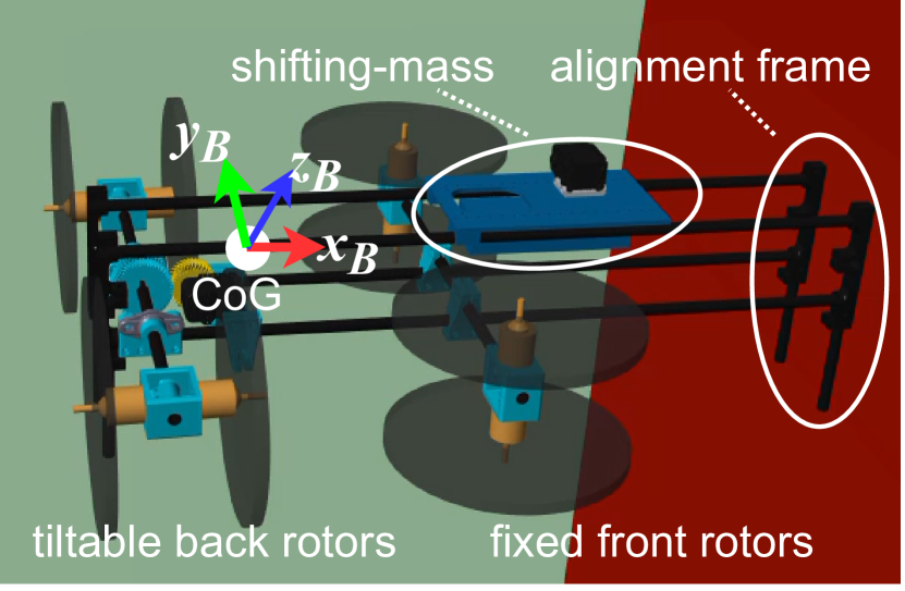
Figure 1: The body frame $\mathcal{F}^{B}=\{O_{B};\bm{x}_{B},\bm{y}_{B},\bm{z}_{B}\}$ is attached to the cog of the aerial vehicle. The aerial vehicle pushes on a vertical surface using an alignment frame along the body axis $\bm{x}_{B}$ with tilted back rotors. The system’s com is shifted by moving the shifting-mass towards the work surface while preserving contact using the alignment frame.

The development of aerial manipulators capable of physically interacting with the environment has experienced significant growth over the past decade [2, 5]. The existing multirotors for aerial manipulation typically have a fixed com [10, 11, 20], located within the rotor-defined area. During interactions with a work surface, preventing rotors from contacting the surface is essential to avoid crashes. This is typically achieved by placing the ee at a considerable distance from the rotors, resulting in an extended moment arm between the ee tip and the aerial vehicle’s com.

In [3], the authors demonstrated drilling into a horizontal surface on the ground with an aerial vehicle. The ee for drilling is attached to the bottom part of the aerial vehicle towards the ground. During drilling, the platform weight contributes to the vertical feed force parallel with the gravity force vector. For operations on non-horizontal surfaces that often appear in industrial infrastructures, however, the ee is usually placed on the side of the aerial vehicle to exert horizontal forces (i.e., forces perpendicular to the gravity force vector) to the environment [6]. In these situations, carrying heavy tools at the ee tip presents the challenge of shifting the com sideways from its initial position, potentially leading to instability during free flight. As a solution, a counterweight can be placed on the opposite side of the ee to compensate for this effect [12]. This approach aims at preserving the system’s com at its original location which still features the aforementioned extended moment arm.

Operations such as grinding often involve large forces along the work surface [13]. A greater moment arm between the system’s com and the EE tip results in larger external torques introduced by these forces during interactions. Larger external torques can present high-risk scenarios where the platform’s rotors operate near saturation. Additionally, for aerial vehicles equipped with high-dof manipulators, servo actuators are generally used in the manipulator [12]. To reduce the reaction forces and torques induced by the motion of the manipulator, these servos are usually placed as close as possible to the com of the aerial vehicle [5]. The load generated by the heavy tool’s weight and interaction forces at the ee tip due to the extended moment arm can cause damage to these servos owing to their technical constraints.

Alternatively, perching is a common approach to handle heavy tools and exert significant forces on non-horizontal work surfaces in aerial manipulation applications [14]. While grasping-based perching often entails additional complexity and weight in the system due to grippers for grasping [15, 16, 19], attaching-based perching achieved by magnets, adhesives, and vacuum cups has become popular recently [14, 17, 18, 4]. In [4], the authors introduced a perching and tilting aerial vehicle designed for concrete wall drilling. This aerial vehicle has two suction cups for perching and can bring its fixed com closer to the work surface by maneuvering the aerial vehicle. Ensuring successful perching between the aerial platform and the work surface is pivotal during these operations. However, industrial infrastructures often present complex environments characterized by varying surface flatness, roughness, shape and orientation, air humidity, and other factors [14]. The environmental uncertainties in practice can affect perching robustness, leading to risky conditions.

I-A Main Contribution

To address the challenges in heavy-tool handling on non-horizontal surfaces, we introduce a novel com shifting aerial vehicle. The aerial vehicle adopts the form of a classic coaxial octocopter, with the body frame $\mathcal{F}^{B}=\{O_{B};\bm{x}_{B},\bm{y}_{B},\bm{z}_{B}\}$ attached to its cog, as in fig. 1. The front rotors remain fixed as unidirectional rotors, while the back rotors can tilt along the body axis $\bm{y}_{B}$. This configuration entails the decoupling between horizontal force generation along $\bm{x}_{B}$ and gravity force compensation of the platform. Subsequently, the platform can orient its body around the $\bm{y}_{B}$ axis by tilting the back rotors. This feature enables interactions with non-horizontal surfaces at different orientations using a rigidly attached link, referred to as the alignment frame, as in fig. 1.

In this work, we focus on applications on verticle surfaces using the designed aerial vehicle. We assume that the system’s com coincides with the cog of the aerial vehicle during free flight and can shift along the body axis $\bm{x}_{B}$ during interactions. The com shifting is accomplished by the linear motion of a movable plate equipped with major heavy components, including the manipulator for heavy-tool handling, referred to as the shifting-mass. This article is outlined as the following:

• Section II: the system design of the aerial vehicle and the maximum com displacement.

• Section III and IV: system modeling and control of the designed platform.

• Section V: a self-positioning approach for the shifting-mass to achieve the maximum com displacement.

• Section VI: evaluation of the presented concepts using a simulator that closely captures the developed physical prototype based on the designed aerial vehicle.

• Section VII: conclusion of the work.

II System Design

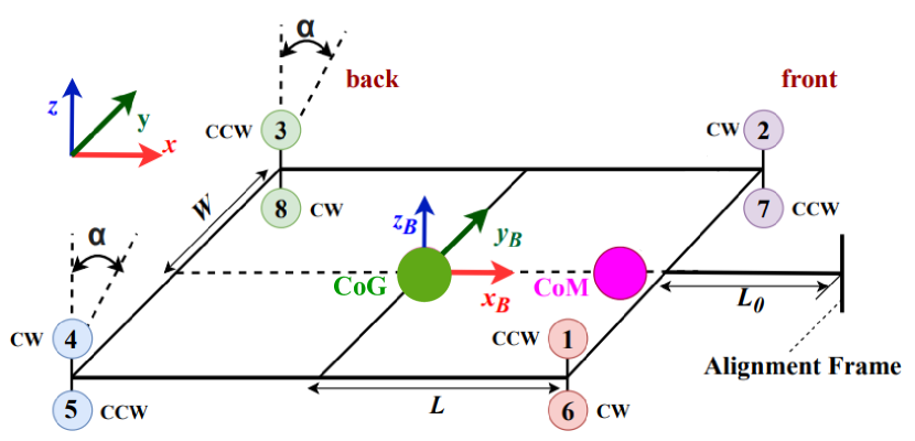
Figure 2: The world frame $\mathcal{F}_{w}=\{\bm{O};\bm{x},\bm{y},\bm{z}\}$ and the body frame $\mathcal{F}^{B}$. The rotating axes of rotors 3, 4, 5, and 8 can tilt simultaneously with angle $\alpha\in[-90\degree,\ 90\degree]$ around $\bm{y}_{B}$, the system’s com can shift along $\bm{x}_{B}$ starting from the cog. CCW: counter-clockwise; CW: clockwise.

In this section, we outline the system design of the aerial vehicle. By positioning the shifting-mass at the cog of the aerial vehicle located within the rotor-defined area, we can assume that the initial com of the system coincides with the cog during free flight. The platform can interact with the environment along $\bm{x}_{B}$, denoted as the interaction axis. An alignment frame, positioned at the front of the aerial vehicle outside the rotor-defined area as in fig. 1, preserves physical contact with the vertical surface while shifting-mass is maneuvered towards the work surface. In the following, we detail the rotor configuration, center-of-mass shifting mechanism, and the maximum com displacement.

II-A Rotor Configuration

The rotor configuration of the aerial vehicle is presented in fig. 2. The aerial vehicle has eight rotors in total. Rotors 1, 2, 6, and 7 in the front have fixed rotating axes parallel to $\bm{z}_{B}$. On the other hand, rotors 3, 4, 5, and 8 have tiltable axes that can simultaneously tilt around $\bm{y}_{B}$ via a servo motor. The tilting angle between the tiltable axis and $\bm{z}_{B}$ is denoted as $\alpha\in[-90\degree,\ 90\degree]$. The tiltable back rotors introduce an additional dof to the system compared to the classic coaxial octocopter with 4-dof actuation. The distance between the cog of the system and each rotor center along $\bm{x}_{B}$ is represented by $L$, while the distance along $\bm{y}_{B}$ is denoted as $W$. $L_{0}$ presents the length of the alignment frame.

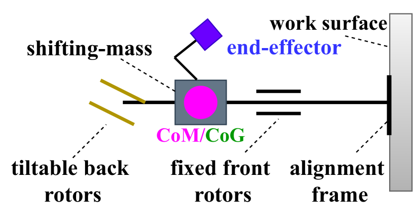
(a)

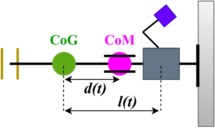
(b)

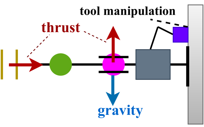
(c)

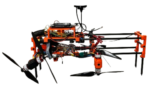
(d)

Figure 3: (a-c) a series of schematics that describes the operational flow of the designed aerial vehicle for tool manipulation on a vertical surface. Step (a) the platform gets into contact with the work surface using the alignment frame via a pushing task; (b) the shifting-mass position $l(t)$ increases until the system’s com location $d(t)$ reaches the maximum value $d=L$ with $l>L$, i.e., the shifting-mass is outside of the rotor-defined area; (c) the back rotors can tilt up to $90\degree$ and the platform can execute tool manipulation closer to the work surface. (d) A physical prototype of the designed aerial vehicle.

II-B Center-of-Mass Shifting

The shifting-mass introduced in section I-A includes the battery, the onboard computer (which can be left out if the product is lightweight), the manipulator with heavy tools at the ee tip, and other mechatronic components. We denote $m_{S},\ m\in\mathbb{R}^{+}$ as the mass of the shifting-mass plate and the total system mass respectively, with $m_{S}<m$. Various types of ees can be attached to the shifting-mass for specific manipulation tasks. The shifting-mass plate is connected to a linear actuator and can move along $\bm{x}_{B}$ starting from the system’s cog up to the alignment frame tip.

The operational flow of the aerial vehicle for tool manipulation on vertical surfaces is presented in fig. 3. The com shifting process is enabled when the system is preserving a stable contact with the work surface using the alignment frame tip, see fig. 3(a) and fig. 3(b). The shifting-mass position along $\bm{x}_{B}$ wrt the cog is denoted as $l(t)\in[0,L+L_{0}]$, as in fig. 3(b). The maximum shifting-mass position is restricted by the alignment frame length $L_{0}$. The resultant displacement of the system’s com along $\bm{x}_{B}$ is denoted by $d(t)$. When the system’s com is located at $d>L$, the aerial vehicle flips around the contact area, leading to instability. Therefore, $d(t)$ is restricted by $[0,L]$. Assuming symmetric mass distribution of the platform around the body axes, the relation between $l(t)$ and $d(t)$ is given by:

$$d(t)=\frac{m_{S}}{m}l(t).$$ (1)

With eq. 1, the maximum com displacement $d=L$ results in a shifting-mass position of $l=\displaystyle\frac{m}{m_{S}}L>L$.

II-C Maximum Center-of-Mass Displacement

Ideally, it is desired to have the system’s com shifted to the maximum displacement $d=L$ during interactions, where the shifting-mass is positioned outside the rotor-defined area towards the work surface, as shown in fig. 3(b). Neglecting friction forces from the work surface, with $d=L$, only front rotors supply the force for gravity compensation while the thrust generated by back rotors can be fully used to exert horizontal interaction forces on the vertical surface with $\alpha=90\degree$, as in fig. 3(c). In this case, the system can entail maximized horizontal force generation on vertical surfaces, and the shortest moment arm between the ee tip and the com for having the shifting-mass closer to the work surface. Consequently, shorter beams can be used for the manipulator, resulting in a more compact design and less weight.

A physical prototype for simple pushing tasks using the alignment frame has been developed, as shown in fig. 3(d). In practice, the mass distribution across the platform is not symmetric around the body axes. Directly moving the shifting-mass with $l=\displaystyle\frac{m}{m_{S}}L$ may lead to the com displacement falling either below $d<L$ or beyond $d>L$. In the former case, the platform cannot achieve the desired configuration in fig. 3(c), while in the latter, instability may arise, resulting in risky situations for the platform. Therefore, later in this article, we propose a method enabling the platform to automatically move its shifting-mass to achieve the maximum com displacement.

III System Modeling

In this section, we present the system modeling of the designed aerial vehicle in section II. We define $\mathcal{F}_{w}=\{\bm{O};\bm{x},\bm{y},\bm{z}\}$ as the world frame, see fig. 2. We denote $T_{i}=k_{t}\Omega_{i}^{2}\in\mathbb{R},i\in[1,8]$ as the thrust magnitude of the $i-th$ rotor, with $k_{t}\in\mathbb{R}$ being the thrust coefficient of the rotors and $\Omega_{i}\in\mathbb{R}^{+}$ being the rotating speed. According to the rotor configuration in fig. 2, the drag torque of the $i-th$ rotor along the positive thrust direction is given by $\tau_{i}=(-1)^{i}k_{b}\Omega_{i}^{2}\in\mathbb{R}$ with $k_{b}\in\mathbb{R}$ being the drag torque coefficient of the rotors. We denote $\bm{R}\in SO(3)$ as the rotation matrix associated with the orientation of the body frame $\mathcal{F}_{B}$ wrt the world frame. The rotation matrix is given by:

$$\bm{R}=\begin{bmatrix}C_{\theta}C_{\psi}&S_{\theta}C_{\psi}S_{\phi}-S_{\psi}C_{\phi}&S_{\theta}C_{\psi}C_{\phi}+S_{\psi}S_{\phi}\\ C_{\theta}S_{\psi}&S_{\theta}S_{\psi}S_{\phi}+C_{\psi}C_{\phi}&S_{\theta}S_{\psi}C_{\phi}-C_{\psi}S_{\phi}\\ -S_{\theta}&C_{\theta}S_{\phi}&C_{\theta}C_{\phi}\end{bmatrix},$$ (2)

where $\phi$, $\theta$, $\psi\in(-90\degree,90\degree)$ are roll-pitch-yaw Euler angles.

III-A Moment of Inertia Estimation

To simplify the modeling, we assume that the body axes of frame $\mathcal{F}_{B}$ correspond with the system’s principal axes of inertia. The inertia matrix of the system $\bm{I}$ expressed in the body frame can be written in the form of $\bm{I}=diag(\begin{bmatrix}I_{xx}&I_{yy}&I_{zz}\end{bmatrix})$. Unlike the conventional UAVs (Unmanned Aerial Vehicles) with fixed centers of mass and constant moments of inertia, while shifting the system’s com along $\bm{x}_{B}$, the moments of inertia along axes $\bm{y}_{B}$ and $\bm{z}_{B}$ vary.

To reduce modeling inaccuracies, we present the moment of inertia estimation associated with $l(t)$. To do so, the geometry, mass, and moments of inertia of the main components used in the physical model in fig. 3(d) are captured by CAD models. Each element in section III-A is measured in Solidworks with realistic CAD models. Shown by the measurements, $I_{xx}=0.0444$$\mathrm{kg}\text{\,}{\mathrm{m}}^{2}$ stays constant for different value of $l$, while $I_{yy}$ and $I_{zz}$ change values along with $l$. Together with obtained measurements, linear regression technology is applied to obtain mathematical models of $I_{yy}$ and $I_{zz}$ wrt $l$. The models are given by:

$$\begin{split}&I_{yy}(l)=0.49l^{2}+0.0538\ ($\mathrm{kg}\text{\,}{\mathrm{m}}^{2}$),\\ &I_{zz}(l)=0.52l^{2}+0.0795\ ($\mathrm{kg}\text{\,}{\mathrm{m}}^{2}$).\end{split}$$ (3)

The estimated inertia matrix of the designed system is thus given by $\bm{I}(l)=diag(\begin{bmatrix}I_{xx}&I_{yy}(l)&I_{zz}(l)\end{bmatrix})$.

III-B System Actuation

We now introduce the actuation wrenches (i.e., forces and torques) of the system generated by rotors configured as in fig. 2. Given the tiltable back rotors, the aerial vehicle can have thrust components along the interaction axis $\bm{x}_{B}$. The actuation force vector $\bm{F}_{a}\in\mathbb{R}^{3}$ expressed in the body frame $\mathcal{F}_{B}$ is given by¹:

$$\bm{F}_{a}=\begin{bmatrix}F_{1}\\ 0\\ F_{3}\end{bmatrix}=\begin{bmatrix}T_{3,4,5,8}S_{\alpha}\\ 0\\ T_{3,4,5,8}C_{\alpha}+T_{1,2,6,7}\end{bmatrix}.$$ (4)

The actuation torque vector $\bm{\Gamma}_{a}\in\mathbb{R}^{3}$ wrt the system’s com expressed in $\mathcal{F}_{B}$ is given by:

$$\bm{\Gamma}_{a}=\begin{bmatrix}(T_{2,7}-T_{1,6}+(T_{3,8}-T_{4,5})C_{\alpha})W+\tau_{3,4,5,8}S_{\alpha}\\ (T_{3,4,5,8})C_{\alpha}(L+d(t))-(T_{1,2,6,7})(L-d(t))\\ (T_{4,5}-T_{3,8})S_{\alpha}W+\tau_{3,4,5,8}C_{\alpha}+\tau_{1,2,6,7}\end{bmatrix}.$$ (5)

The actuation torque vector is in relation with the com displacement $d(t)$, and with eq. 1, we have $\bm{\Gamma}_{a}=\bm{\Gamma}_{a}(l)$. Based on eq. 4 and eq. 5, the system has 9 inputs with 5-dof actuation. The system inputs are the rotors’ rotating speed and back rotors’ tilting angle, i.e., $\bm{u}=\begin{bmatrix}\alpha&\Omega_{1}&\Omega_{2}&\Omega_{3}&\Omega_{4}&\Omega_{5}&\Omega_{6}&\Omega_{7}&\Omega_{8}\end{bmatrix}^{\top}\in\mathbb{R}^{9}$.

III-C Equations of Motion

Assuming the slow motion of the movable plate and tilting axes, we neglect the dynamics of the linear actuator for shifting-mass and the servo for tilting back rotors. The system equations of motion expressed in the body frame $\mathcal{F}_{B}$ can be written as:

$$\begin{bmatrix}\bm{M}&\bm{0}\\ \bm{0}&\bm{I}(l)\end{bmatrix}\begin{bmatrix}\dot{\bm{\upsilon}}\\ \dot{\bm{\omega}}\end{bmatrix}+\begin{bmatrix}\bm{\omega}\times\bm{M}\bm{\upsilon}\\ \bm{\omega}\times\bm{I}(l)\bm{\omega}\end{bmatrix}+\bm{G}=\begin{bmatrix}\bm{F}_{a}\\ \bm{\Gamma}_{a}(l)\end{bmatrix}+\begin{bmatrix}\bm{F}_{C}\\ \bm{\Gamma_{C}}\end{bmatrix},$$ (6)

where $\bm{M}\in\mathbb{R}^{3\times 3}$ is the mass matrix, $\bm{\upsilon}\in\mathbb{R}^{3}$ is the linear velocity vector of the body frame $\mathcal{F}_{B}$ wrt the world frame origin, $\bm{\omega}\in\mathbb{R}^{3}$ is the angular velocity vector of the body frame $\mathcal{F}_{B}$ wrt the world frame. We use $S(\bm{a})\in\mathbb{R}^{3\times 3}$ to present the skew symmetric matrix such that $S(\bm{a})\bm{b}=\bm{a}\times\bm{b}$, and we have $\dot{\bm{R}}=\bm{\omega}\times\bm{R}=S(\bm{\omega})\bm{R}$. We define the operator $(\cdot)^{\vee}$ such that $\bm{a}=S(\bm{a})^{\vee}$. We denote $\begin{bmatrix}\bm{F}_{C}\\ \bm{\Gamma_{C}}\end{bmatrix}\in\mathbb{R}^{6}$ as the stacked force and torque vector from the environment to the system assuming that the interaction wrenches at the end-effector and alignment frame tip are the only sources of external wrenches, $\bm{G}\in\mathbb{R}^{6}$ is the gravity term expressed in the body frame $\mathcal{F}_{B}$.

IV Control Design

In this section, we present the control design of the aerial vehicle introduced in section II to handle both free flight and physical interactions during a pushing task. Considering the underactuation of the modeled system as introduced in section III-B, inspired by [9, 20, 21] a cascade control structure is applied, see Fig. 4.

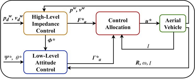
Figure 4: Control Design.

The control structure involves a low-level geometric attitude controller, a high-level selective impedance controller, and control allocation. The impedance and attitude controllers output the desired actuation wrenches by tracking references of linear and angular motion. The actuation wrenches are achieved by varying the rotating speed of rotors $\Omega_{i}$ and the tilting angle $\alpha$, i.e., system inputs $\bm{u}$, which are calculated in the control allocation. In the following, we detail each part of the control design.

IV-A Low-level Geometric Attitude Control

The low-level attitude controller outputs the desired actuation torques by tracking the system’s orientation and angular velocity in the body frame. We use the geometric controller introduced in [21] to control the system’s attitude dynamics. $\phi^{*}$, $\theta^{*}$ and $\psi^{*}$ present the desired Euler angles. We denote $\bm{R}_{d}(\phi^{*},\theta^{*},\psi^{*})\in SO(3)$ as the reference rotation matrix and $\bm{\omega}_{d}\in\mathbb{R}^{3}$ as the reference angular velocity vector expressed in the body frame. The attitude tracking error $\bm{e}_{R}\in\mathbb{R}^{3}$ is defined as $\bm{e}_{R}=\frac{1}{2}(\bm{R}_{d}^{\top}\bm{R}-\bm{R}^{\top}\bm{R}_{d})^{\vee},$ and the angular velocity tracking error $\bm{e}_{\omega}\in\mathbb{R}^{3}$ is defined as: $\bm{e}_{\omega}=\bm{\omega}-\bm{R}^{\top}\bm{R}_{d}\bm{\omega}_{d}$.

A nonlinear feedback controller for attitude dynamics is designed as:

$$\begin{split}\bm{\Gamma}_{a}^{*}=&-\bm{K}_{R}\bm{e}_{R}-\bm{K}_{\omega}\bm{e}_{\omega}+\bm{\omega}\times\bm{I}(l)\bm{\omega}\\ &-\bm{I}(l)(S(\bm{\omega})\bm{R}^{\top}\bm{R}_{d}\bm{\omega}_{d}-\bm{R}^{\top}\bm{R}_{d}\dot{\bm{\omega}}_{d}),\end{split}$$ (7)

where $\bm{K}_{R}$ and $\bm{K}_{\omega}\in\mathbb{R}^{3\times 3}$ are positive-definite matrices. $\bm{\Gamma}_{a}^{*}$ is the desired actuation torque vector, which is then fed to the control allocation together with the desired actuation force vector from the high-level impedance controller, as in fig. 4.

IV-B High-level Selective Impedance Control

The high-level selective impedance control outputs the desired actuation forces by tracking the position and velocity references of the aerial vehicle in the world frame. This control strategy prevents switching controllers between free flight and physical interactions for pushing. More specifically, we track the body frame origin of $O_{B}$ attached to the aerial vehicle’s cog, instead of the shifting-mass. We now express the linear dynamics of the system in the world frame as:

$$\bm{M}\dot{\bm{\upsilon}}^{w}+\bm{\omega}^{w}\times\bm{M}\bm{\upsilon}^{w}+mg\bm{e}_{3}=\bm{F}_{a}^{w}+\bm{F}_{C}^{w},$$ (8)

where $g=-9.81$$\mathrm{m}\text{\,}{\mathrm{s}}^{-2}$, $\bm{e}_{3}=\begin{bmatrix}0&0&1\end{bmatrix}^{\top}$, $\bm{F}_{a}^{w}=\bm{R}\bm{F}_{a}$ and $\bm{F}_{C}^{w}=\bm{R}\bm{F}_{C}$. With eq. 2, $\bm{F}_{a}^{w}$ is given by:

$$\bm{F}_{a}^{w}=\begin{bmatrix}C_{\theta}C_{\psi}F_{1}+(S_{\theta}C_{\psi}C_{\phi}+S_{\psi}S_{\phi})F_{3}\\ C_{\theta}S_{\psi}F_{1}+(S_{\theta}S_{\psi}C_{\phi}-C_{\psi}S_{\phi})F_{3}\\ -S_{\theta}F_{1}+C_{\theta}C_{\phi}F_{3}\end{bmatrix}.$$ (9)

We define $\bm{p}^{w}_{d}\in\mathbb{R}^{3}$ as the desired position of $O_{B}$ expressed in the world frame. The position tracking error is given by $\bm{e}_{p}^{w}=\bm{p}^{w}-\bm{p}^{w}_{d}$, where $\bm{p}^{w}\in\mathbb{R}^{3}$ represents the position of the origin $O_{B}$ wrt $O$ expressed in the world frame. The velocity tracking error can then be displayed as $\bm{e}_{v}^{w}=\bm{\upsilon}^{w}-\bm{\upsilon}^{w}_{d}$ with $\bm{\upsilon}^{w}_{d}=\dot{\bm{p}}^{w}_{d}$. The desired close loop dynamics of the system with the selective impedance control is:

$$\bm{M}\dot{\bm{e}}_{v}^{w}+\bm{D}\bm{e}_{v}^{w}+\bm{K}\bm{e}_{p}^{w}=\bm{F}_{C}^{w},$$ (10)

where $\bm{D}$ and $\bm{K}\in\mathbb{R}^{3\times 3}$ are positive-definite matrices representing the desired damping and stiffness of the system. With eq. 8 and eq. 10, the desired actuation force vector expressed in the world frame is defined as:

$$\begin{split}\bm{F}_{a}^{w*}&=\begin{bmatrix}F_{1}^{w*}&F_{2}^{w*}&F_{3}^{w*}\end{bmatrix}^{\top}\\ &=\bm{M}\dot{\bm{\upsilon}}_{d}^{w}-\bm{D}\bm{e}_{v}^{w}-\bm{K}\bm{e}_{p}^{w}+\bm{\omega}^{w}\times\bm{M}\bm{\upsilon}^{w}+mg\bm{e}_{3}.\end{split}$$ (11)

While the thrust generated by the rotors does not have a component along $\bm{y}_{B}$ of the body frame, the system introduces coupling between its roll angle $\phi$ and the linear motion in the world frame. With the control output from the high-level impedance control in eq. 11, we can calculate the desired roll angle $\phi^{*}$ using eq. 9 to have $\bm{F}_{a}^{w*}=\bm{F}_{a}^{w}$ by:

$$\begin{split}\phi^{*}=&atan2\big{(}S_{\psi}F_{1}^{w*}-C_{\psi}F_{2}^{w*},S_{\theta}C_{\psi}F_{1}^{w*}+...\\ &S_{\theta}S_{\psi}F_{2}^{w*}+C_{\theta}F_{3}^{w*}\big{)}.\end{split}$$ (12)

Furthermore, by using trigonometric calculations with eq. 9, the desired actuation force vector $\bm{F}_{a}^{*}=\begin{bmatrix}F_{1}^{*}&0&F_{3}^{*}\end{bmatrix}$ expressed in the body frame is given by:

$$F_{1}^{*}=C_{\theta}C_{\psi}F_{1}^{w*}+C_{\theta}S_{\psi}F_{2}^{w*}-S_{\theta}F_{3}^{w*},$$ (13a)

$$\begin{split}F_{3}^{*}=&\big{(}(S_{\psi}F_{1}^{w*}-C_{\psi}F_{2}^{w*})^{2}+(S_{\theta}C_{\psi}F_{1}^{w*}+...\\ &S_{\theta}S_{\psi}F_{2}^{w*}+C_{\theta}F_{3}^{w*})^{2}\big{)}^{\frac{1}{2}}.\end{split}$$ (13b)

The desired roll angle $\phi^{*}$ is then fed to the low-level attitude controller with other attitude references $\psi^{*}$ and $\theta^{*}$. The attitude controller tracks the desired rotation matrix $\bm{R}_{d}(\phi^{*},\theta^{*},\psi^{*})$ and outputs the desired actuation torque vector $\bm{\Gamma}_{a}^{*}$ in the body frame. The desired actuation wrenches $\bm{F}_{a}^{*}$ and $\bm{\Gamma}_{a}^{*}$ in the body frame are then fed to the control allocation to derive the desired system inputs $\bm{u}^{*}$, as in fig. 4.

IV-C Control Allocation

The control allocation finds the rotating speed of each rotor and the tilting angle of the back rotors’ rotating axes to achieve the desired actuation wrenches. Applying the method used in [22], we introduce a virtual control vector $\bm{\lambda}\in\mathbb{R}^{12}$ representing each component of the thrust vectors generated by rotors along the body frame axes as:

$$\begin{split}\bm{\lambda}=&(\lambda_{1},\ \lambda_{2},\ ...,\ \lambda_{12})^{\top}\\ =&(\Omega^{2}_{1},\ \Omega^{2}_{2},\ \Omega^{2}_{3}C_{\alpha},\ \Omega^{2}_{3}S_{\alpha},\ \Omega^{2}_{4}C_{\alpha},\ \Omega^{2}_{4}S_{\alpha},...\\ &\Omega^{2}_{5}C_{\alpha},\ \Omega^{2}_{5}S_{\alpha},\ \Omega^{2}_{6},\Omega^{2}_{7},\ \Omega^{2}_{8}C_{\alpha},\ \Omega^{2}_{8}S_{\alpha})^{\top}.\end{split}$$ (14)

With the desired actuation wrench vector $\begin{bmatrix}\bm{F}_{a}^{*}\\ \bm{\Gamma}_{a}^{*}\end{bmatrix}\in\mathbb{R}^{6}$ from the impedance and attitude controllers, by applying eq. 1, eq. 4 and eq. 5 the allocation between the desired wrenches and the desired virtual input vector $\bm{\lambda}^{*}$ is given by:

$$\begin{bmatrix}\bm{F}_{a}^{*}\\ \bm{\Gamma}_{a}^{*}\end{bmatrix}=\bm{H}(l)\cdot\bm{\lambda}^{*},$$ (15)

where $\bm{H}(l)\in\mathbb{R}^{6\times 12}$ is an allocation matrix that depends on the shifting-mass position $l(t)$ wrt $O_{B}$ and does not depend on the tilting angle $\alpha$. With eq. 15, the desired virtual control vector is calculated via pseudo-inverse by applying:

$$\bm{\lambda}^{*}=\bm{H}(l)^{{\dagger}}\cdot\begin{bmatrix}\bm{F}_{a}^{*}\\ \bm{\Gamma}_{a}^{*}\end{bmatrix},$$ (16)

where $(\cdot)^{{\dagger}}$ is the pseudo-inverse operator. From $\bm{\lambda}^{*}$ the desired real system inputs $\bm{u}^{*}$ can be derived by:

$$\begin{split}\bm{u}^{*}=&\Big{[}atan2(\lambda_{12}^{*},\lambda_{11}^{*})\ \sqrt{\lambda_{1}^{*}}\ \sqrt{\lambda_{2}^{*}}\ \sqrt[4]{{\lambda_{3}^{*}}^{2}+{\lambda_{4}^{*}}^{2}}...\\ &\sqrt[4]{{\lambda_{5}^{*}}^{2}+{\lambda_{6}^{*}}^{2}}\ \sqrt[4]{{\lambda_{7}^{*}}^{2}+{\lambda_{8}^{*}}^{2}}\ \sqrt{\lambda_{9}^{*}}\ \sqrt{\lambda_{10}^{*}}\ \sqrt[4]{{\lambda_{11}^{*}}^{2}+{\lambda_{12}^{*}}^{2}}\Big{]}^{\top}.\end{split}$$ (17)

The calculated system inputs are sent to the aerial vehicle. The aerial vehicle provides state feedback used in the control design and the shifting-mass position used for the moment of inertia estimation in eq. 3 and control allocation in eq. 16.

V Shifting-mass Self-positioning

In this section, we present a shifting-mass self-positioning process to automatically find the optimal shifting-mass position such that the system’s com reaches its maximum displacement $d=L$ as in fig. 3(b) and fig. 3(c). This process is executed while the platform is pushing a verticle surface using the alignment frame.

The optimal shifting-mass position can be found when back rotors are tilted with the maximum value of $\alpha=90\degree$. With the high-level impedance control in section IV-B, the platform can exert a force along the interaction axis $\bm{x}_{B}$ to the work surface with a position reference “behind” the work surface. To achieve maximum tilting angle $\alpha$ during interactions, significant horizontal force generation on the vertical surface is required from the aerial system by setting a proper position reference. During the self-positioning, while the system is exerting a horizontal force on the vertical surface using the alignment frame, the shifting-mass position is feedback controlled using the tilting angle $\alpha$ to reach $\alpha=90\degree$ and is given by:

$$l=k_{\alpha}e_{\alpha},$$ (18)

where $e_{\alpha}=90\degree-\alpha$ is the tracking error, $k_{\alpha}$ is a positive gain.

Once the shifting-mass position reaches a steady state with $\alpha=90\degree$, we determine the optimal shifting-mass position, denoted as $l^{*}$, for the current setup. This process occurs only once per setup, after which the shifting-mass is directly commanded to move until it reaches $l=l^{*}$ for tool operations. This self-positioning process should be performed whenever there are changes in manipulators or other components affecting the system’s mass distribution, essentially serving as a calibration step. Considering the physical constraints imposed by the alignment frame’s length, it is preferable to ensure $l^{*}<L+L_{0}$ in hardware design to maximize the com displacement, as discussed in section II-C.

VI Numerical Results and Discussion

In this section, we test the presented system through simulations that closely emulate the physical platform displayed in fig. 3(d). To achieve this, we utilize a Simscape model, as in fig. 1, which corresponds to the developed physical prototype, in the subsequent tests. The control design outlined in section IV and the self-positioning approach described in section V are implemented in Simulink. The tests include both free-flight evaluations and physical interactions. Specifically, the physical interaction task involves exerting force against a vertical surface using only the alignment frame. Our future endeavors aim to explore aerial manipulation applications employing various ees. In the following sections, we detail the executed tests.

VI-A Free-Flight Tests

Free-flight tests were conducted to evaluate the tracking on both position and attitude references of the designed system. Firstly, a set of pitch references was sent to the system, while the references of other rotation angles and linear velocities were zeros. With the tiltable back rotors, the aerial vehicle can vary its pitch angle in a range of $[-70\degree,70\degree]$, as shown in fig. 5 (a).

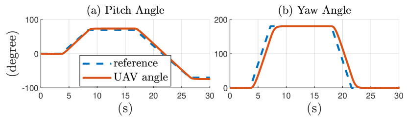
Figure 5: The (a) pitch reference and UAV pitch angle, (b) yaw reference and UAV yaw angle.

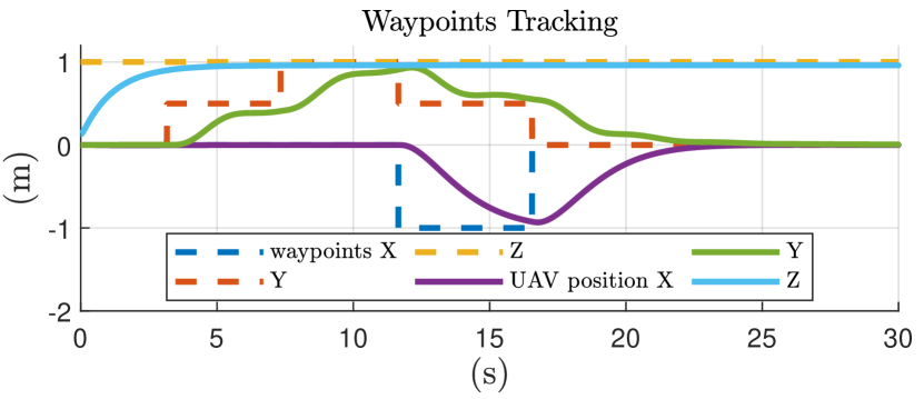
Figure 6: The waypoints to be tracked and the UAV position.

Similarly, a set of yaw references was sent to the system and the aerial vehicle can vary its yaw angle in the range of $[-180\degree,180\degree]$, as shown in fig. 5 (b). Furthermore, a series of waypoints was used to test the position control while yaw and pitch references were zeros, see fig. 6. The testing results show promising orientation and position control of the designed system during free flight.

VI-B Physical Interaction Tests

In this section, we present the testing results for physical interactions that involve a pushing task on a vertical surface. The shifting-mass self-positioning process was executed during the pushing task. A set of waypoints which include the points “behind” the work surface were sent to the high-level impedance controller to make the aerial vehicle approach and contact the work surface using the alignment frame. Once stable contact between the alignment frame and the work surface was obtained, the shifting-mass self-positioning was enabled. The shifting-mass position $l$ increased along the body axis $\bm{x}_{B}$ starting from its initial value $l=0$$\mathrm{m}$ while the back rotors tilting angle $\alpha$ was increasing, see fig. 7 Zone 1.

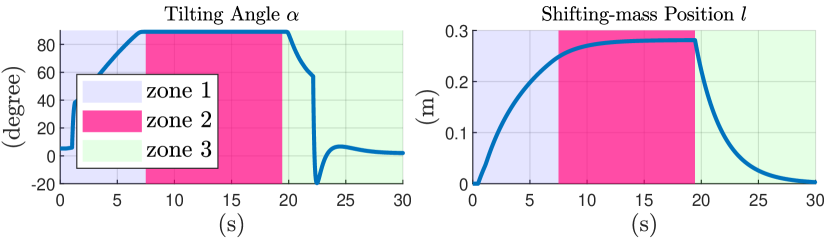
Figure 7: The (a) tilting angle $\alpha$ and (b) shifting-mass position $l$ while the platform is interacting with the vertical work surface. Zone 1: the shifting-mass self-positioning process was enabled while the alignment frame was preserving contact with the work surface. The shifting-mass moved along positive $\bm{x}_{B}$ starting from its initial position $l=0$$\mathrm{m}$ while the tilting angle $\alpha$ was increasing. Zone 2: the shifting-mass position reached $l=0.25$$\mathrm{m}$ with $\alpha\approx 90\degree$ and kept increasing until it reached a steady state at $l^{*}=0.281$$\mathrm{m}$. The self-positioning was completed and the com reached the maximum displacement. Zone 3: the shifting-mass returned to its initial position while the tilting angle $\alpha$ was decreasing.

In Zone 2, the self-positioning of the shifting-mass was completed with $\alpha\approx 90\degree$. During this, the shifting-mass reached a position at $l=0.25$$\mathrm{m}$ and kept increasing until the optimal position at $l^{*}=0.281$$\mathrm{m}$. It maintained this position while exerting horizontal forces on the vertical surface using the full thrust of back rotors. After the self-positioning process, the shifting-mass came back to its initial position, as in Zone 3. The determined optimal shifting-mass position $l^{*}$ from the simulation can assist the hardware design to have the alignment frame length $L_{0}>l^{*}-L$, which allows the maximum com displacement. The executed tests are shown in the attached video, also available at https://youtu.be/f4pSGr39C68.

VI-C Discussion

In practice, the system’s state feedback required for the control design is typically acquired through external sensors like IMUs and motion capture systems. The shifting-mass position $l(t)$ required for the allocation matrix in eq. 15 and moment of inertia estimation in eq. 3 can also be obtained via motion capture systems or actuator information. The feedback on tilting angle $\alpha$ required for the shifting-mass self-positioning in eq. 18 can be acquired via the Dynamixel servos used in the physical prototype. The proposed methods thus guarantee the future physical implementation.

Determining a proper position reference is essential to ensure that the back rotors achieve maximum tilting angle during the shifting-mass self-positioning process. Moreover, the gain value $k_{\alpha}$ is pivotal and needs adjustment when there are changes in mass distribution. Simulations aid in identifying a suitable position reference and $k_{\alpha}$ for the self-positioning process, mitigating potential risks during practical experiments and preventing platform damage. From fig. 7, a range of $l\in[0.25\ 0.281]$$\mathrm{m}$ can enable $\alpha\approx 90\degree$ instead of a single value of $l^{*}$. However, further analysis is warranted, taking into account friction forces on the work surface.

VII Conclusion

In this study, we introduced a novel aerial vehicle designed specifically for shifting its com to handle heavy tools on non-horizontal surfaces. Maximizing the com displacement towards the work surface is critical for enhancing the platform’s horizontal force generation on vertical surfaces while reducing the moment arm between the ee tip and the system’s com. To achieve this, we proposed a method to automatically determine the shifting-mass position, allowing the equipped manipulator to operate closer to the work surface. We validated our proposed concepts through simulations that closely replicate the developed physical model. With this work, we introduced promising future avenues for a new class of aerial vehicles in enhanced tool manipulation applications.

References

- [1] Bogue, R. (2018), ”What are the prospects for robots in the construction industry?”, Industrial Robot, Vol. 45 No. 1, pp. 1-6. https://doi-org.proxy.findit.cvt.dk/10.1108/IR-11-2017-0194.
- [2] F. Ruggiero, V. Lippiello and A. Ollero, ”Aerial Manipulation: A Literature Review,” in IEEE Robotics and Automation Letters, vol. 3, no. 3, pp. 1957-1964, July 2018, doi: 10.1109/LRA.2018.2808541.
- [3] Y. Sun, A. Plowcha, M. Nail, S. Elbaum, B. Terry and C. Detweiler, ”Unmanned Aerial Auger for Underground Sensor Installation,” 2018 IEEE/RSJ International Conference on Intelligent Robots and Systems (IROS), Madrid, Spain, 2018, pp. 1374-1381, doi: 10.1109/IROS.2018.8593824.
- [4] R. Dautzenberg et al., ”A Perching and Tilting Aerial Robot for Precise and Versatile Power Tool Work on Vertical Walls,” 2023 IEEE/RSJ International Conference on Intelligent Robots and Systems (IROS), Detroit, MI, USA, 2023, pp. 1094-1101, doi: 10.1109/IROS55552.2023.10342274.
- [5] A. Ollero, M. Tognon, A. Suarez, D. Lee and A. Franchi, ”Past, Present, and Future of Aerial Robotic Manipulators,” in IEEE Transactions on Robotics, vol. 38, no. 1, pp. 626-645, Feb. 2022, doi: 10.1109/TRO.2021.3084395.
- [6] T. Bartelds, A. Capra, S. Hamaza, S. Stramigioli and M. Fumagalli, ”Compliant Aerial Manipulators: Toward a New Generation of Aerial Robotic Workers,” in IEEE Robotics and Automation Letters, vol. 1, no. 1, pp. 477-483, Jan. 2016, doi: 10.1109/LRA.2016.2519948.
- [7] Trujillo, M.Á.; Martínez-de Dios, J.R.; Martín, C.; Viguria, A.; Ollero, A. Novel Aerial Manipulator for Accurate and Robust Industrial NDT Contact Inspection: A New Tool for the Oil and Gas Inspection Industry. Sensors 2019, 19, 1305. https://doi.org/10.3390/s19061305
- [8] R. Watson et al., ”Dry Coupled Ultrasonic Non-Destructive Evaluation Using an Over-Actuated Unmanned Aerial Vehicle,” in IEEE Transactions on Automation Science and Engineering, vol. 19, no. 4, pp. 2874-2889, Oct. 2022, doi: 10.1109/TASE.2021.3094966.
- [9] C. Ding and L. Lu, ”A Tilting-Rotor Unmanned Aerial Vehicle for Enhanced Aerial Locomotion and Manipulation Capabilities: Design, Control, and Applications,” in IEEE/ASME Transactions on Mechatronics, vol. 26, no. 4, pp. 2237-2248, Aug. 2021, doi: 10.1109/TMECH.2020.3036346.
- [10] S. Kim, S. Choi and H. J. Kim, ”Aerial manipulation using a quadrotor with a two DOF robotic arm,” 2013 IEEE/RSJ International Conference on Intelligent Robots and Systems, Tokyo, Japan, 2013, pp. 4990-4995, doi: 10.1109/IROS.2013.6697077.
- [11] H. -N. Nguyen, S. Park, J. Park and D. Lee, ”A Novel Robotic Platform for Aerial Manipulation Using Quadrotors as Rotating Thrust Generators,” in IEEE Transactions on Robotics, vol. 34, no. 2, pp. 353-369, April 2018, doi: 10.1109/TRO.2018.2791604.
- [12] F. Ruggiero et al., ”A multilayer control for multirotor UAVs equipped with a servo robot arm,” 2015 IEEE International Conference on Robotics and Automation (ICRA), Seattle, WA, USA, 2015, pp. 4014-4020, doi: 10.1109/ICRA.2015.7139760.
- [13] M.A. Elbestawi, K.M. Yuen, A.K. Srivastava, H. Dai, Adaptive Force Control for Robotic Disk Grinding, CIRP Annals, Volume 40, Issue 1, 1991, Pages 391-394, ISSN 0007-8506, https://doi.org/10.1016/S0007-8506(07)62014-9.
- [14] Meng J, Buzzatto J, Liu Y, Liarokapis M. On Aerial Robots with Grasping and Perching Capabilities: A Comprehensive Review. Front Robot AI. 2022 Mar 25;8:739173. doi: 10.3389/frobt.2021.739173.
- [15] S. B. Backus, L. U. Odhner and A. M. Dollar, ”Design of hands for aerial manipulation: Actuator number and routing for grasping and perching,” 2014 IEEE/RSJ International Conference on Intelligent Robots and Systems, Chicago, IL, USA, 2014, pp. 34-40, doi: 10.1109/IROS.2014.6942537.
- [16] H. Zhang, J. Sun and J. Zhao, ”Compliant Bistable Gripper for Aerial Perching and Grasping,” 2019 International Conference on Robotics and Automation (ICRA), Montreal, QC, Canada, 2019, pp. 1248-1253, doi: 10.1109/ICRA.2019.8793936.
- [17] L. Daler, A. Klaptocz, A. Briod, M. Sitti and D. Floreano, ”A perching mechanism for flying robots using a fibre-based adhesive,” 2013 IEEE International Conference on Robotics and Automation, Karlsruhe, Germany, 2013, pp. 4433-4438, doi: 10.1109/ICRA.2013.6631206.
- [18] H. W. Wopereis, T. D. van der Molen, T. H. Post, S. Stramigioli and M. Fumagalli, ”Mechanism for perching on smooth surfaces using aerial impacts,” 2016 IEEE International Symposium on Safety, Security, and Rescue Robotics (SSRR), Lausanne, Switzerland, 2016, pp. 154-159, doi: 10.1109/SSRR.2016.7784292.
- [19] A. McLaren, Z. Fitzgerald, G. Gao and M. Liarokapis, ”A Passive Closing, Tendon Driven, Adaptive Robot Hand for Ultra-Fast, Aerial Grasping and Perching,” 2019 IEEE/RSJ International Conference on Intelligent Robots and Systems (IROS), Macau, China, 2019, pp. 5602-5607, doi: 10.1109/IROS40897.2019.8968076.
- [20] K. Bodie et al., “An omnidirectional aerial manipulation platform for contact-based inspection,” in Proc. Robot.: Sci. Syst., 2019.
- [21] T. Lee, et al. Control of Complex Maneuvers for a Quadrotor UAV using Geometric Methods on SE(3), 2010. https://doi.org/10.48550/arxiv.1003.2005.
- [22] M. Kamel et al., ”The Voliro Omniorientational Hexacopter: An Agile and Maneuverable Tiltable-Rotor Aerial Vehicle,” in IEEE Robotics & Automation Magazine, vol. 25, no. 4, pp. 34-44, Dec. 2018, doi: 10.1109/MRA.2018.2866758.