tcb@breakable
An Active Perception Game for Robust Autonomous Exploration
Abstract
We††General Robotics, Automation, Sensing and Perception (GRASP) Laboratory, University of Pennsylvania. Email: {siminghe, yztao, igorspas, kumar, pratikac}@seas.upenn.edu formulate active perception for an autonomous agent that explores an unknown environment as a two-player zero-sum game: the agent aims to maximize information gained from the environment while the environment aims to minimize the information gained by the agent. In each episode, the environment reveals a set of actions with their potentially erroneous information gain. In order to select the best action, the robot needs to recover the true information gain from the erroneous one. The robot does so by minimizing the discrepancy between its estimate of information gain and the true information gain it observes after taking the action. We propose an online convex optimization algorithm that achieves sub-linear expected regret for estimating the information gain. We also provide a bound on the regret of active perception performed by any (near-)optimal prediction and trajectory selection algorithms. We evaluate this approach using semantic neural radiance fields (NeRFs) in simulated realistic 3D environments to show that the robot can discover up to 12% more objects using the improved estimate of the information gain. On the M3ED dataset, the proposed algorithm reduced the error of information gain prediction in occupancy map by over 67%. In real-world experiments using occupancy maps on a Jackal ground robot, we show that this approach can calculate complicated trajectories that efficiently explore all occluded regions.
![[Uncaptioned image]](/html/2404.00769/assets/x1.png)
I INTRODUCTION
As robots transition from controlled laboratory environments into real-world settings, their ability to comprehend their surroundings becomes increasingly crucial. This ability will enable robots to plan and make decisions in complex environments adaptively. There is an increase of research interest in active perception [1, 2]. Active perception algorithms can be crucial in search and rescue, planetary exploration, environmental monitoring, structure inspection, etc.
Active perception is commonly formulated as finding a control sequence that maximizes the information gained from the environment. This requires the agent to predict the information gain of putative actions. Typically, this is done on the basis of some map that the robot builds using past observations. The “true” information gained is the incremental information from the actual realized future observations. Of course, the robot could never correctly estimate this true information gain a priori. But it can compare the estimated information gain before each observation to the true information gained after the observation, to build a better estimate for the next episode. This paper develops an approach to do so, and, as a consequence, obtain a robust active perception pipeline that ekes out more from potentially poor past exploratory actions. We formulate the active perception problem as a two-player zero-sum game between the agent and the environment as illustrated and explained in Fig. 1. An introductory video along with the experiments can be accessed at: https://youtu.be/p7Elon583q4.
The contributions of our paper are as follows:
-
•
We formulate robust active perception as a two-player zero-sum game between the agent and the environment in Section II. Then, we prove the regret bound on active perception performance given any (near-)optimal prediction and trajectory selection algorithms in Section IV-C.
-
•
We present a robust active perception algorithm to make and improve information gain prediction online in Section III. We prove this algorithm has a sub-linear expected regret for prediction in Section IV-B.
-
•
As shown in Section V, we integrate the proposed algorithms into two different active perception systems that use semantic NeRF and occuppancy maps respectively. Then, we conduct extensive experiments 1) in a photorealistic simulator, 2) on the M3ED dataset, and 3) on a customized Clearpath Jackal platform. The experiments demonstrate the effectiveness and generalizability of the proposed method.
I-A Related Work
Related works have studied active perception systems based on different scene representations. Each representation has its unique application and challenges in the context of active perception.
I-A1 Gaussian Processes (GP)
Active sensing in GP has been well studied in [3]. Finding optimal sensor placement is an NP-complete problem. The work obtains near-optimal online bounds for greedy algorithms based on the submodularity of mutual information (MI). The analysis assumes GP has a known covariance function which is usually unrealistic in real-world applications. An extension [4] uses a near-optimal exploration-exploitation approach for stationary GP with an unknown covariance function. For non-stationary GP, a single estimation of covariance function is not enough. The paper [4] proposed manually dividing the whole space into smaller areas with a stationary process. Then, a similar analysis also gives an efficient and near-optimal algorithm for informative path planning in GP [5, 6, 7].
These works provide a near-optimal performance guarantee when the covariance function and MI prediction are easy and accurate. However, many robotics tasks require more complicated representations such as non-stationary GP, occupancy map, point cloud, or semantic map. In those representations, different regions could have very different and diverse characteristics. It’s unrealistic to model every small area one by one. In addition, the observation model could be unclear in semantic and implicit representations. As a result, the mutual information prediction could be inaccurate, and the performance guarantee would not hold. To bridge this gap, our paper firstly establishes the relationship between mutual information prediction loss and performance guarantee of active perception. Then, we provide an online algorithm with a expected regret guarantee on the prediction loss.
I-A2 Occupancy Map
Occupancy map is commonly used in robotics tasks. Due to the complicated nature of such representation, most active perception algorithms with occupancy maps don’t provide performance guarantee analysis. Next-best-views (NBV) methods samples and selects viewpoint that maximizes some utility functions. Utilities based on the amount of observed volume is used in [8, 9, 10]. The following works [11, 12] used surface reconstruction utility in addition to volumetric utility. Information-theoretic methods [13, 14, 15] design efficient algorithms to calculate mutual information between range sensor data and occupancy maps. Since the occupancy of unseen areas is unknown, NBV and information-theoretic methods could underestimate or overestimate the utility. To address this issue, several works [16, 17, 18] propose map completion. The methods train neural networks to predict the occupancy of unseen areas based on existing datasets. Those methods work well in environments similar to the datasets but would struggle in out-of-distribution environments. Hence, the methods could not guarantee a general algorithm performance at test time. In contrast, based on online learning algorithm, our method provides performance guarantees at test time even in out-of-distribution or adversarial environments.
I-A3 Semantic and Implicit representation
Semantic scene representations become popular in recent years and have been used for loop-closure, navigation, and decision making. Uncertainty in semantics [19, 20, 21] is used as a utility for exploration. Our theory and algorithm can be applied to the methods and provide performance guarantees. Reinforcement learning methods [22, 23, 24] are also used for active perception by learning to act based on past data. Unlike those methods, our method will not struggle in out-of-distribution environments.
II Problem Formulation
We will first discuss the formal description of the active perception game. We consider a sequential game between Nature and the robot that evolves over episodes as follows. At the start, Nature selects a scene that is unknown to the robot but is kept fixed throughout the game. In each episode, , Nature selects and reveals to the robot vantage points and the erroneous information gain that these viewpoints provide about the unknown scene . Let be the set of all measures that the robot could obtain from each of the locations respectively. The robot selects a subset of points in subject to some budget constraints and collects measurements
from each of these viewpoints. We use to denote the set of observations in episode , i.e., from the -th to the -th observation in all collected observations. Using these observations, the robot can calculate the true information gain of these locations . The game then transitions to the subsequent episode with Nature revealing a new set of candidate vantage points and their erroneous information gain, and so on… The game ends after episodes. The history of measurements of the agent in episode is then
The protocol of the game is summarized in Definition II.1. The objective of the agent is to maximize the amount of true information gain collected about the environment. In the following sections, we describe in more detailed notions such as accuracy, map measurements, and a suitable notion of (approximate) optimality. We use to denote the hidden quantity of interest, such as the map of the environment. If we did not have any observations, the scene is drawn from a probability distribution . If we have past observations , it tells us that the scene will be drawn from a more concentrated distribution .
Definition II.1 (Active Perception Game)
For episodes :
-
0.
Nature selects , together with and a erroneous version for , where is the power set of .
-
1.
With budget constraints, robot selects a subset of observations based on context which consists of , , and .
-
2.
Robot receives measurements and after visiting points .
The information gain is defined as the mutual information between past and future observations:
where . The task of the agent is to develop a policy to minimize
| (1) |
which is equivalent to maximize
| (2) |
where each can be regarded as a mapping of the following form .
III Active Perception Algorithm
Active perception aims at obtaining information of the scene through control of an agent. We can formalize it as selecting control sequences to maximize the mutual information in each episode
| (3) |
The mutual information objective depends on selected future observations which is determined by the control . Since we don’t know true information gain beforehand, the agent makes an estimate of the true information gain based on the erroneous . The estimate is based on the improvement function
| (4) |
Then, the agent maximizes .
Remark III.1
The erroneous information gain could be any estimate of the actual information gain. Therefore, our method is a general way that can be applied to numerous existing active perception systems that predict . For many active perception systems, the predictions are usually inaccurate due to (a) complexity of scene representation; (b) aleatoric uncertainty from unmodeled sensor noise; (c) assumption of independent observations.
We show in Section IV that our algorithms have no-regret predictions of information gain. This leads to a bounded regret for active perception performance.
III-A Information Gain Prediction
An agent can make prediction based on erroneous information gain by IPO (Improving Prediction Online) in Algorithm 1. At the end of each episode, the agent also learns to make better prediction by LIP (Learning to Improve Prediction) in Algorithm 2.
We firstly explain the notations we used in the algorithms. For episode and , let
| (5) |
By chain rule, we have . Similarly, we define and .
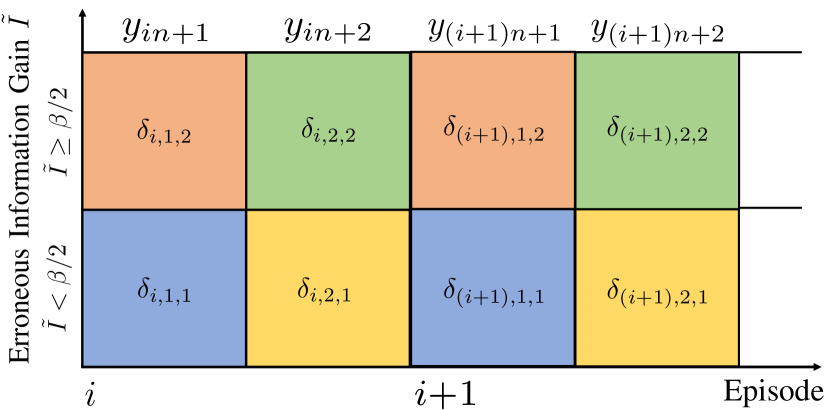
The subgroup and improvement function could be any reasonable function. Considering the generalization and the sample complexity of our algorithms, we choose classes of functions that are simple but effective. We illustrate our choices in Fig. 2.
Definition III.1 (Subgroup Function )
Assuming is in , we discretize to bins. The initial prediction is in the -th bin if . For , we define subgroup function such that
| (6) |
Definition III.2 (Improvement Function )
The function is defined as
| (7) |
is a learned constant to improve the predictions at -th bin at episode for subgroup .
We use value of initial prediction as context because it is closely related to the notion of multicalibration which guarantees low errors even when conditioned on initial predictions [25]. Initial prediction usually assumes the independence of observations . To reduce prediction errors due to this assumption, the improvement also depends on . We could choose different subgroup definition for prediction improvement. The analysis and implementation can be easily extended to other definitions of and .
Since we have a set of pixel-wise mutual information feedback at each time in real applications, we use the notation to denote a set of mutual information feedback at time . We are improving the mutual information prediction of each pixel. We also use the notation in LIP. keeps track of the number of past updates in each subgroup. is the number of times that predictions are in subgroup (j,k) up to and including episode . is the learning rate and is the gradient of loss.
In IPO, we want to return a set of mutual information predictions at each pixel. The algorithm directly applies our to get each prediction from erroneous information gain.
In LIP, ) returns the (sub)gradient of loss . From line 12 to line 17, the algorithm refines the improvement function by updating .
Input , improvement function
Output improved prediction
Input ,
improvement function , number of updates
Output ,
III-B Informative Path Planning
Optimizing over the objective Eq. 3 is known to be NP-complete and many approximation algorithms have been proposed to achieve near-optimality with tractable runtime [3].
Input prediction mechanism , optimization oracle ,
randomization level
Output the selected future observations
In episode , we denote the policy to find the that maximizes predicted information gain given prediction mechanism , i.e.,
The information gain given this policy is
| (8) |
Using is feasible for a small set of sampled observations since we can find by iterating through all possible . For larger set of sampled observations, approximation algorithm for the policy has to be used. For example, the eSIP algorithm in [5] is proved to satisfy
In general, our algorithm and analysis work for any such that
IPP in Algorithm 3 takes in an optimization oracle and the prediction mechanism . Line 2 stores the selected path. For each observation on the path, we sample from a uniform distribution in line 3. We denote the j-th observation. In line 5, with probability , we set to be a randomly selected observation from . controls the amount of randomization (exploration) by our algorithm.
III-C Combined Algorithm
In Algorithm 4, we integrate IPO, IPP, LIP into the active perception system. Given the context from Nature (line 3), the agent uses information gain prediction to select measurements (line 4 and 5) to observe. After observing the measurements and receiving true information gain (line 6), the agent learns to improve prediction (line 8).
IV Analysis
Though our algorithms are based on pixel-wise mutual information feedback , we assume single pixel observation and mutual information feedback at each time step in this analysis section for conciseness. The analysis and conclusion would be the same up to constant terms.
IV-A Regret for Online Prediction with Full Information
Our problem is in bandit-feedback setting (i.e., only receive true information gain for observed views). We firstly analyze our algorithm in full-information setting (i.e., receive true information gain for all views in ). Then, we show a reduction from bandit-feedback setting to full-information setting. In full-information setting, we set .
Since each subgroup is improved independently, we start by analyzing a single subgroup . The number of predictions in subgroup in episode is
and the total predictions in the subgroup is
for full-information setting. We denote
the set of predictions that are in subgroup in episode . This is different from the notation in previous section, but note that
is a partition of all predictions
Online prediction in full-information setting is an online convex optimization problem: for each episode and subgroup , Nature chooses a convex loss by selecting all , then the agent selects predictions to minimize the loss. The convex loss is
| (9) |
We define regret as the performance measure. When the agent finishes episode and looks back, it realizes is the prediction that it should have made. Regret is the additional loss due to predicting instead of .
Definition IV.1 (Subgroup Prediction Regret)
For and , we have subgroup prediction regret
| (10) |
where is the loss when
| (11) |
The overall regret is
| R | (12) |
An algorithm is said to be no-regret if the average regret as . Follow the leader algorithms solve online convex optimizations by selecting the best past prediction as the next prediction [26]. Regularization is usually added to the algorithms to avoid oscillatory prediction. We firstly show that our LIP algorithm is a special case of follow the regularized leader in Lemma VI.1. Then, we provide the regret bound of this special case in Lemma VI.2.
By choosing a suitable scheduler of the learning rate, we can obtain the sub-linear regret of the proposed algorithm
Theorem IV.1
LIP uses learning rate . The regret bound with this learning rate is
And the bound on R is in worst case
Proof:
Plug in the specified to the bound in Lemma VI.2. is bounded due to Holder’s inequality . R is bounded by Jensen’s inequality. ∎
Remark IV.1
Our online prediction algorithm with IPO and LIP has no-regret since and goes to 0 as .
IV-B Regret for Online Prediction with Bandit Feedback
We follow the similar process in [27] to reduce bandit-feedback setting to full-information setting. With bandit feedback, the agent can only observe part of the loss that is corresponding to where is the -th observed (information gain, observation) in subgroup in episode . For , is observed with probability . To use the full-information algorithm in Section IV-A for bandit-feedback problem, we firstly need to hallucinate the loss. Let be the hallucination for the -th loss in episode for subgroup . For ,
| (13) |
We show this filled loss is unbiased Lemma VI.3 which is important for analyzing regret in expectation. Additionally, to make this filled loss well-defined, we need to be strictly positive for all . We achieve this by creating a randomized of . Let in LIP. The -th element of equals to the -th element of with probability . With probability , we let the -th element of be randomly sampled from . This randomization gives strictly positive probability for observing each observation as shown in Lemma VI.4. Intuitively, in bandit-feedback setting where the agent cannot collect true information gain for all observations in , the agent needs to explore (by randomization) to understand the true information gain of different observations.
After randomizing LIP, we prove the expected regret in bandit-feedback setting in Lemma VI.5. With a suitable randomization level, the algorithms have a sublinear regret.
Theorem IV.2
Let . The upper bound of expected regret is
Proof:
Plug in the specified into the bound in Lemma VI.5. ∎
Remark IV.2
The randomized algorithm is no-regret in bandit-feedback setting.
IV-C Regret Bound for Robust Active Perception
We want to understand the relationship among quality of information gain predictions, optimality of path planning algorithms, and performance of active perception in this section. Let’s denote the prediction of competitor where each is based on Eq. 11. Assume that 1) the overall regret R is upper-bounded by ; 2) the performance of competitor is upper-bounded by . For concise notations, we will use without in the following section.
We define the regret of active perception as the extra information gain if the agent makes decision based on instead of . We firstly show that improved predictions of information gain lead to a tighter bound on the regret of active perception.
Theorem IV.3
The bound is shown in Theorem IV.2 to be sub-linear in episodes . The bound depends on the capacity of the competitor class. Since the competitor class can choose predictions in hindsight, the bound should be linear in with a small factor given a suitable competitor class. Additionally, we want to take the optimality of path planning algorithms into account.
Theorem IV.4 (Active Perception Performance)
Assume we use a policy in IPP such that
where is described in Section IV-C. The regret of active perception with IPP is
| (15) |
This regret is upper bounded by
See Proof in Section VI-B.
Remark IV.3
If we are using the brute force algorithm , the regret guarantee is
And if we are using the eSIP algorithm , the regret guarantee is
by plugging in the for eSIP.
V RESULTS
To evaluate the effectiveness and generalizability of our method, we conducted three sets of experiments: (1) we evaluated our method in a photorealistic simulator; (2) we studied the effectiveness of our method with noisy sensor measurements using a real-world dataset; (3) we carried out real-world experiments with our algorithms running fully onboard the robot.
V-A Simulation Experiment
| Scene 102344529 | Scene 102344280 | Scene 102344250 | Scene 102816036 | |||||
|---|---|---|---|---|---|---|---|---|
| Loss1 | #Objects2 | Loss | #Objects | Loss | #Objects | Loss | #Objects | |
| Baseline | 86 35.4 | 55 0.8 | 43 5.0 | 381.6 | 57 6.5 | 32 2.9 | 118 13.5 | 66.3 1.2 |
| Improved | 52 15.1 | 55 0.8 | 35 2.6 | 38.7 1.2 | 46 5.0 | 35.3 0.9 | 86 8.1 | 74.3 2.9 |
-
1
The loss of cumulative information gain prediction.
-
2
The number of objects found.
V-A1 Experiment Setup
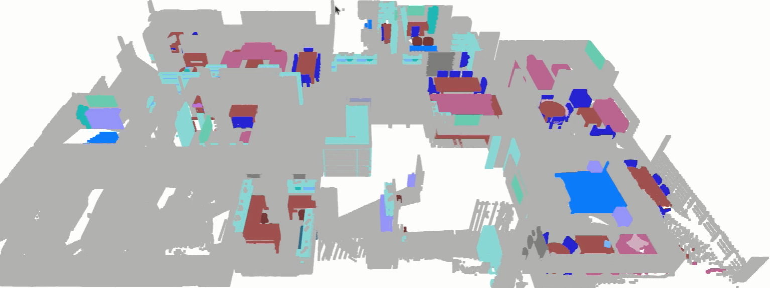
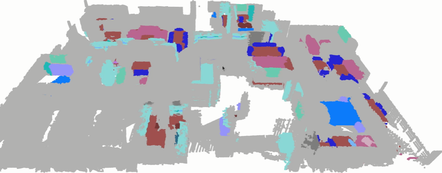
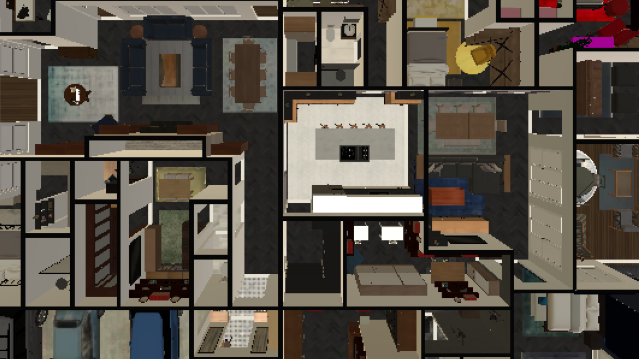
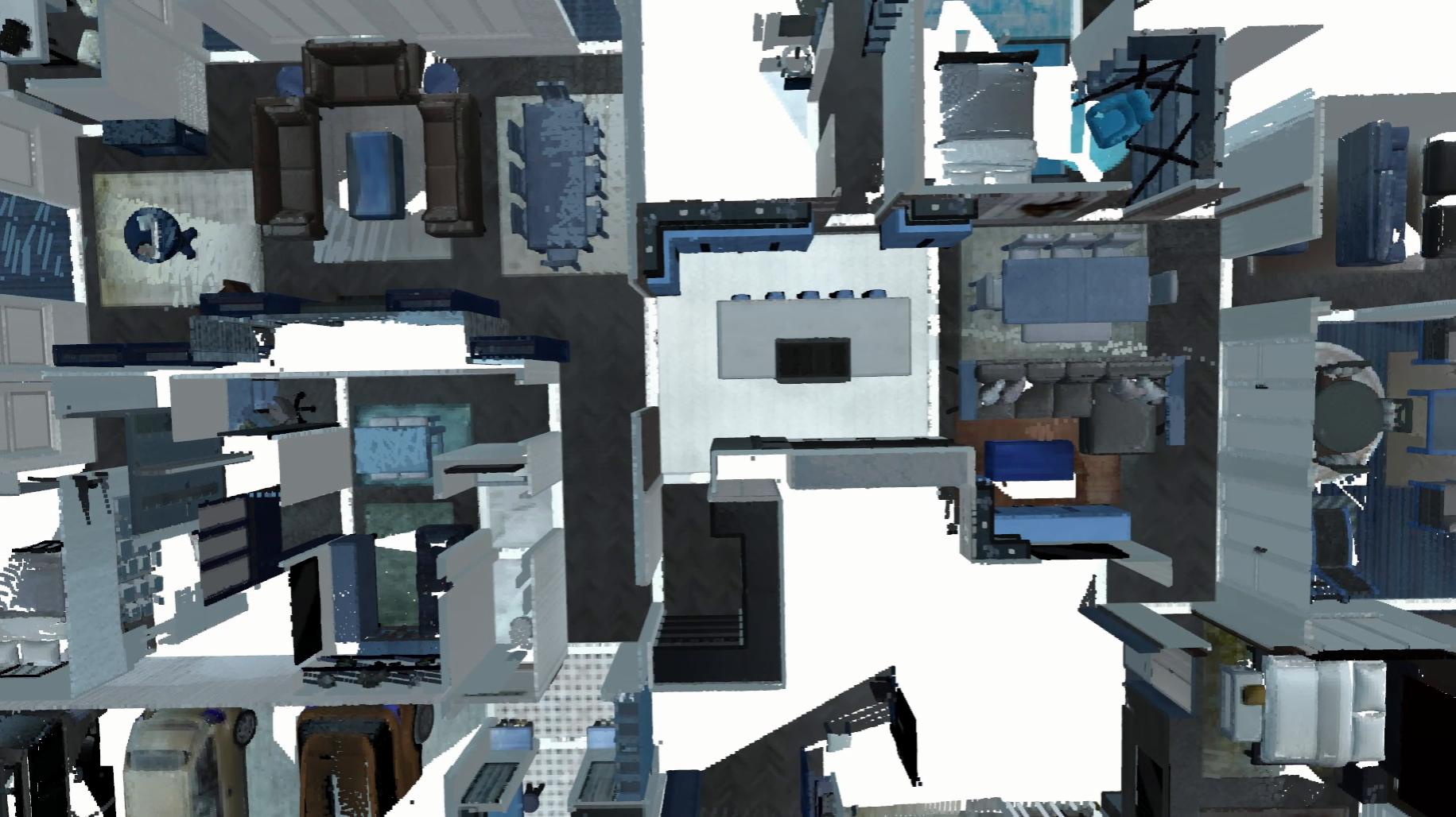
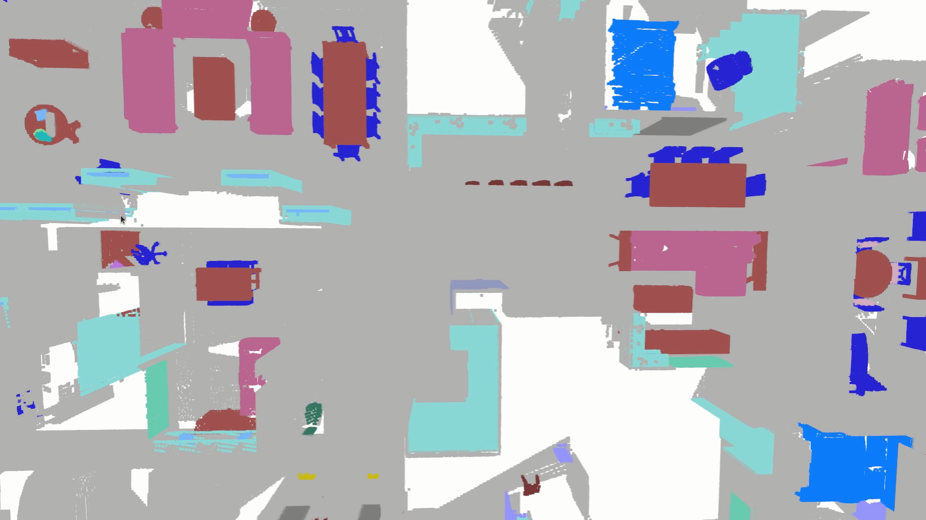
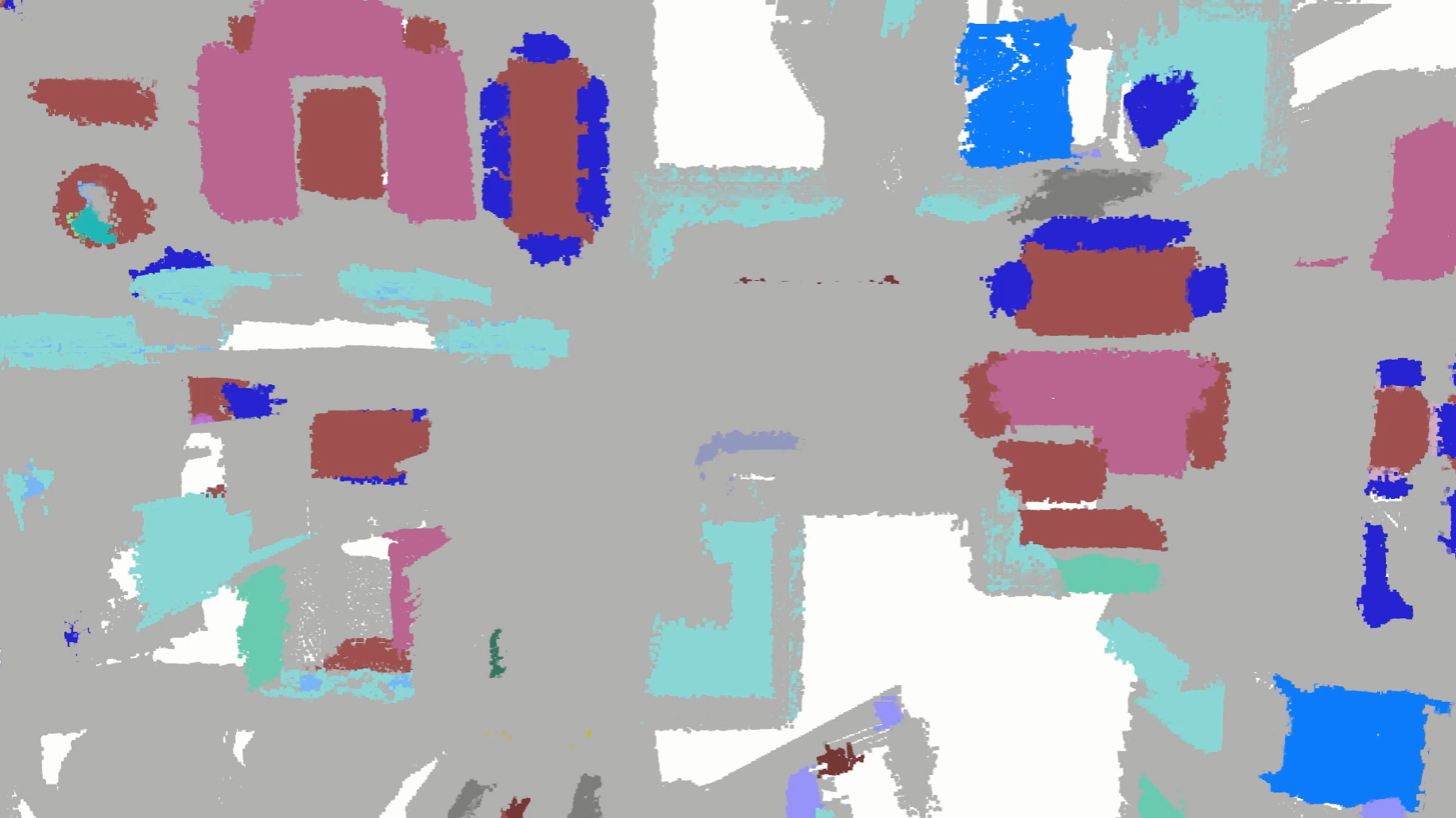
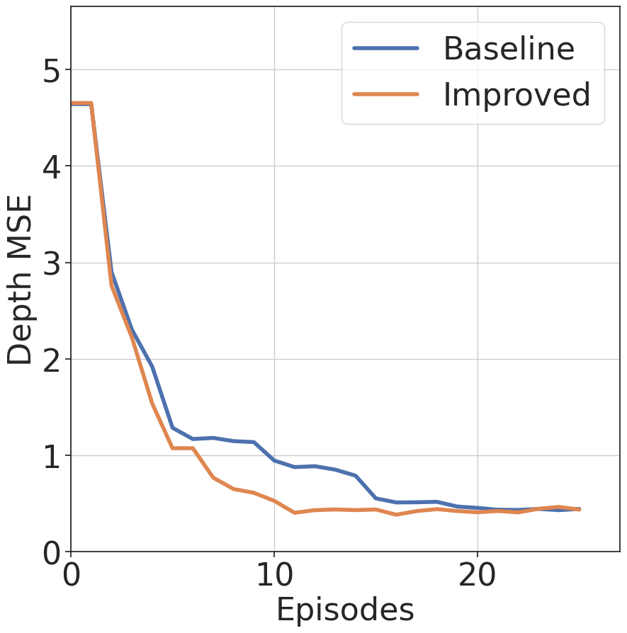
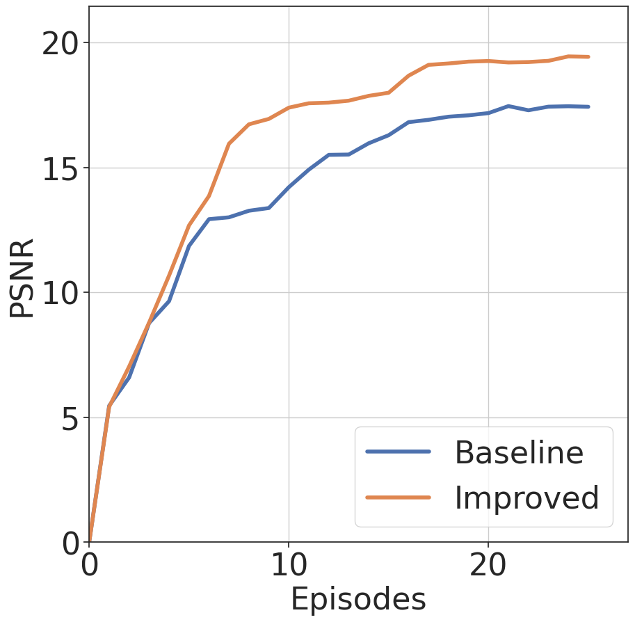
The 3D photorealistic Habitat-Sim [28, 29, 30] is used for our simulation experiments. RGBD images and semantic segmentations are used to train a semantic NeRF during exploration [20]. In all of the simulation experiments, the robot started at a random location in the map and collects an initial set of observations to build the map. Then, we uniformly sampled 20 goals on the x-y plane and generated the paths with Dijkstra’s algorithm. We discretized the path with steps and evaluated the information at each step. The path with the highest aggregated information was passed into Rotorpy [31] to generate a dynamically feasible trajectory for execution.
We use a deep ensemble of NeRFs as in Section II. The includes RGB images, depth measurements, semantic segmentation, and transmittance. For RGB and depth, we model each ray in as a Gaussian distribution where and are estimated from the ensemble [20]. Hence, . Since the entropy depends on which could be arbitrarily large, we set an upper limit to the entropy in practice. In all NeRF experiments, we set the upper bound of the mutual information to be 5. Semantic segmentation generates a distribution over the categories for entropy calculation. We also set the upper bound of the mutual information of segmentation to be . Transmittance of a ray is a Bernoulli random variable of whether the ray hits obstacles. Hence, we set the upper bound of the mutual information of transmittance to be . In this setting, we have six categories of information gain corresponding to RGBD, segmentation, and transmittance. We improve the information prediction in each of the category independently using our algorithms. We choose the number of bins in Definition III.1 to be 100 and the number of measurements in Section II to be 40. Our algorithm generates the aggregated information prediction for each sampled path and executes the one that maximizes it.
After the execution of a path, we update the map based on collected observations . Since we assume the absolute certainty in the observation, observed is a Dirac-delta distribution which is non-zero only at the observations’ value. The feedback is computed as using collected observations from the episode. Given the erroneous information gain, agent’s improved predictions, and the feedback, we can refine the improvement function following LIP. The level of randomization is set to in practice since randomized path is costly for SWaP-constrained agents.
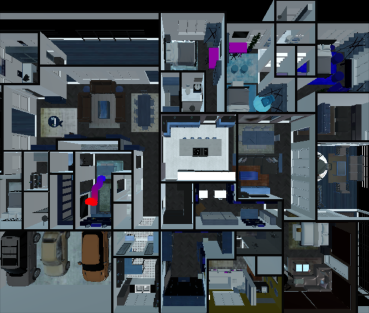
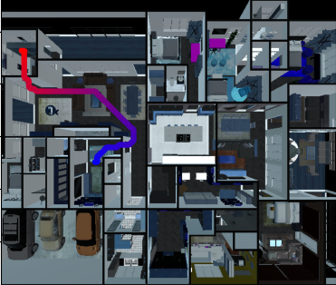
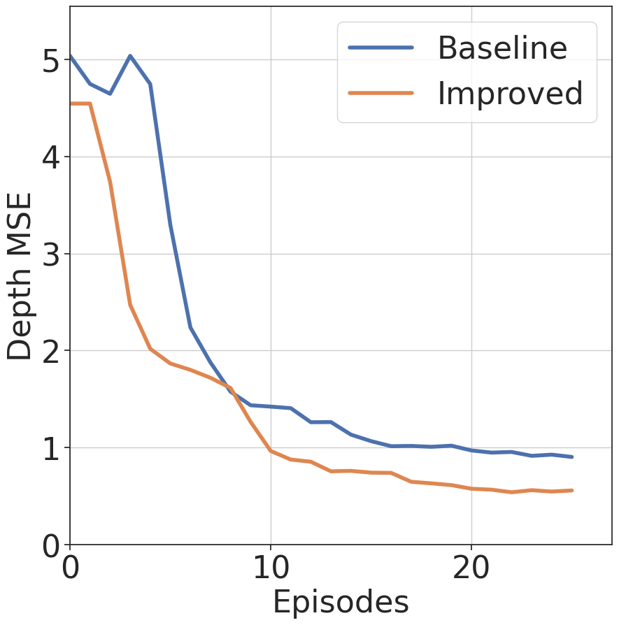
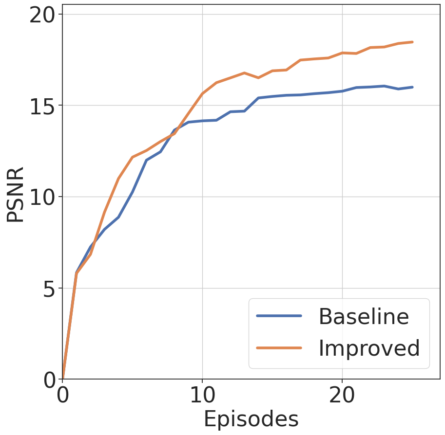
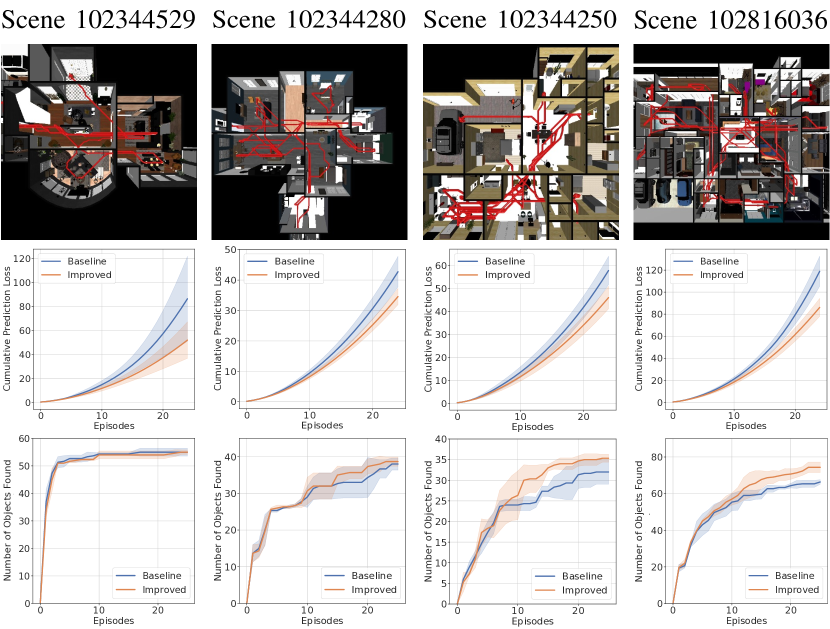
V-A2 Experiment Results
We tested our method in four different simulation environments of varying sizes and complexities. For each experiment, we calculated the cumulative loss of information gain prediction, which is defined as the absolute difference between the information prediction and the feedback. Besides, the number of objects observed during the experiment was recorded. As a result, the proposed method was capable of generating more accurate information predictions and selecting paths that provide observations of more semantic objects, as illustrated in Fig. 3 and Table I. From the statistics of the experiments, the proposed method reduced the error of information gain prediction by 18.6% - 40.0% on average and enabled the robot to observe up to 12% more objects. We envision the improvements will be more significant with the increase in the scale and complexity of the environments.
V-B M3ED Dataset Experiment
| Indoor: building_loop | Outdoor: penno_short_loop | |||||
|---|---|---|---|---|---|---|
| Noise Type | None | Gaussian | Impulse | None | Gaussian | Impulse |
| Baseline | 0.475 | 0.484 | 0.490 | 0.474 | 0.484 | 0.488 |
| Improved | 0.163 | 0.160 | 0.162 | 0.162 | 0.163 | 0.172 |
V-B1 Experiment Setup
We carried out experiments with a high-quality synchronized dataset M3ED [32] to study the performance of our method on information gain prediction under unmodeled sensor noise. In these experiments, we treated the raw lidar data and the associated odometry as the ground truth. We added Gaussian noises and Impulse noises to the ground truth measurements separately to simulate unmodeled sensor noises. Specifically, we applied Gaussian noise with zero mean and standard deviation that equals of the raw depth measurements. For Impulse noise, we replaced half of the measurements with new measurements that are uniformly sampled between and of the original value.
We represented the environment with 3D voxels and assumed they were independent of each other. All voxels were initialized with a probability of occupancy to be . For each measurement and its associated odometry, ray-castings were conducted, followed by a log-odds-based map update. To predict the information gain, rays were uniformly sampled at each position. For each ray that intersects with voxels in , we calculated . Since each ray maximally intersects with voxels, we normalized mutual information to better fit this with our algorithms. We summed up the information of all sampled rays and treated this as the information gain of the observation .
After every observation, we calculated the feedback information gain and the mean prediction loss between the prediction and the feedback. Subsequently, we followed the process described in LIP to improve future information predictions. We set , , and here for our algorithms in Section III-A.
V-B2 Experiment Results
Results in Table II demonstrate that our proposed algorithm significantly improved the accuracy of the prediction of information gain given unmodeled sensor noises. In particular, the prediction loss was reduced by over 67%. This set of experiments demonstrates that the proposed method is capable of providing more accurate information gain prediction even with unmodeled sensor noises.
V-C Real World Experiment
V-C1 Experiment Setup
To validate the effectiveness of our proposed method, we carried out real-world experiments by deploying it on a customized Clearpath Jackal platform. Details of our platform can be found in [33]. The Jackal UGV is equipped with an AMD Ryzen 3600 CPU and an NVIDIA GTX 1650 GPU. In addition, it carries an Ouster OS1-64 LiDAR. We used Faster-LIO [34] for state estimation and move-base [35] for global and local planning. In all our real-world experiments, we used the same map representations and the definition of information gain as described in Section V-B. To reduce computational overhead and enable real-time onboard operations, we set steps to be . In each episode, we sampled an grid centered around the robot with cell length meters. Then we predicted the information gain at each cell lattice. The path with the maximum predicted information gain is searched with DFS on the grid with a max length of 10 meters. Similar to simulation experiments, we set to .
V-C2 Experiment Results
We carried out experiments in both an indoor environment and an urban outdoor environment. One representative result in each environment is shown in Fig. 1. In the indoor environment Fig. 1(a), the robot actively navigated to the regions that are occluded from its start position to perceive more information. Similarly, as shown in outdoor environment in Fig. 1(b), the robot actively navigated to occluded areas that have high actual information gain. Areas that correspond to high information gain from the plot are highlighted. With the proposed algorithm running online, the robot was able to actively plan paths to maximize the gathered information, resulting in full coverage of areas with high information content.
VI DISCUSSION
Active exploration of unknown environments is a challenging task. Fundamentally, this is because the robot does not have an accurate model of the environment to explain its observations, and as a consequence, its estimated information gain is incorrect. We developed an online learning approach to incrementally refine the estimated information gain. We showed, across simulation experiments, evaluations on real-world datasets, and experiments on real robotic platforms, that this approach not only improves the estimate of information gain, but also enables robust active perception policies that can explore new environments effectively. These approaches are essential good real-world performance in applications such as search and rescue missions in unknown environments.
References
- [1] J. A. Placed, J. Strader, H. Carrillo, N. Atanasov, V. Indelman, L. Carlone, and J. A. Castellanos, “A survey on active simultaneous localization and mapping: State of the art and new frontiers,” 2023.
- [2] R. Zeng, Y. Wen, W. Zhao, and Y.-J. Liu, “View planning in robot active vision: A survey of systems, algorithms, and applications,” 2020.
- [3] A. Krause, A. Singh, and C. Guestrin, “Near-optimal sensor placements in gaussian processes: Theory, efficient algorithms and empirical studies,” J. Mach. Learn. Res., vol. 9, 2008.
- [4] A. Krause and C. Guestrin, “Nonmyopic active learning of gaussian processes: an exploration-exploitation approach,” in Proceedings of the 24th international conference on Machine learning, 2007.
- [5] A. Singh, A. Krause, C. Guestrin, and W. J. Kaiser, “Efficient informative sensing using multiple robots,” J. Artif. Int. Res., vol. 34, no. 1, 2009.
- [6] J. Binney and G. S. Sukhatme, “Branch and bound for informative path planning,” in IEEE International Conference on Robotics and Automation, 2012.
- [7] A. Viseras, D. Shutin, and L. Merino, “Robotic active information gathering for spatial field reconstruction with rapidly-exploring random trees and online learning of gaussian processes,” Sensors, vol. 19, no. 5, 2019.
- [8] C. Connolly, “The determination of next best views,” in IEEE International Conference on Robotics and Automation, vol. 2, 1985.
- [9] A. Bircher, M. Kamel, K. Alexis, H. Oleynikova, and R. Siegwart, “Receding horizon ”next-best-view” planner for 3d exploration,” in IEEE International Conference on Robotics and Automation, 2016.
- [10] L. Yoder and S. Scherer, Autonomous Exploration for Infrastructure Modeling with a Micro Aerial Vehicle. Cham: Springer International Publishing, 2016.
- [11] R. Border, J. D. Gammell, and P. Newman, “Surface edge explorer (see): Planning next best views directly from 3d observations,” in IEEE International Conference on Robotics and Automation, 2018.
- [12] L. Schmid, M. Pantic, R. Khanna, L. Ott, R. Siegwart, and J. Nieto, “An efficient sampling-based method for online informative path planning in unknown environments,” IEEE Robotics and Automation Letters, vol. 5, no. 2, 2020.
- [13] Z. Zhang, T. Henderson, V. Sze, and S. Karaman, “Fsmi: Fast computation of shannon mutual information for information-theoretic mapping,” in International Conference on Robotics and Automation, 2019.
- [14] B. Charrow, S. Liu, V. Kumar, and N. Michael, “Information-theoretic mapping using cauchy-schwarz quadratic mutual information,” in IEEE International Conference on Robotics and Automation, 2015.
- [15] T. Henderson, V. Sze, and S. Karaman, “An efficient and continuous approach to information-theoretic exploration,” in IEEE International Conference on Robotics and Automation, 2020.
- [16] R. Shrestha, F.-P. Tian, W. Feng, P. Tan, and R. Vaughan, “Learned map prediction for enhanced mobile robot exploration,” in International Conference on Robotics and Automation, 2019.
- [17] Y. Tao, E. Iceland, B. Li, E. Zwecher, U. Heinemann, A. Cohen, A. Avni, O. Gal, A. Barel, and V. Kumar, “Learning to explore indoor environments using autonomous micro aerial vehicles,” 2023.
- [18] Y. Tao, Y. Wu, B. Li, F. Cladera, A. Zhou, D. Thakur, and V. Kumar, “Seer: Safe efficient exploration for aerial robots using learning to predict information gain,” in IEEE International Conference on Robotics and Automation, 2023.
- [19] G. Georgakis, B. Bucher, K. Schmeckpeper, S. Singh, and K. Daniilidis, “Learning to map for active semantic goal navigation,” 2022.
- [20] S. He, C. D. Hsu, D. Ong, Y. S. Shao, and P. Chaudhari, “Active perception using neural radiance fields,” 2023.
- [21] Y. Tao, X. Liu, I. Spasojevic, S. Agarwal, and V. Kumar, “3d active metric-semantic slam,” IEEE robotics & automation letters., vol. 9, no. 3, 2024-3.
- [22] A. Dosovitskiy and V. Koltun, “Learning to act by predicting the future,” 2017.
- [23] X. Sun, Y. Wu, S. Bhattacharya, and V. Kumar, “Multi-agent exploration of an unknown sparse landmark complex via deep reinforcement learning,” 2022.
- [24] D. S. Chaplot, D. Gandhi, S. Gupta, A. Gupta, and R. Salakhutdinov, “Learning to explore using active neural slam,” 2020.
- [25] I. Globus-Harris, D. Harrison, M. Kearns, A. Roth, and J. Sorrell, “Multicalibration as boosting for regression,” 2023.
- [26] A. Roth, “Learning in games,” 2023. [Online]. Available: https://www.cis.upenn.edu/~aaroth/GamesInLearning.pdf
- [27] A. Slivkins, “Lecture notes: Bandits, experts and games (lecture 8),” 2016. [Online]. Available: https://www.cs.umd.edu/~slivkins/CMSC858G-fall16/lecture8-both.pdf
- [28] M. Savva, A. Kadian, O. Maksymets, Y. Zhao, E. Wijmans, B. Jain, J. Straub, J. Liu, V. Koltun, J. Malik, D. Parikh, and D. Batra, “Habitat: A Platform for Embodied AI Research,” in Proceedings of the IEEE/CVF International Conference on Computer Vision, 2019.
- [29] A. Szot, A. Clegg, E. Undersander, E. Wijmans, Y. Zhao, J. Turner, N. Maestre, M. Mukadam, D. Chaplot, O. Maksymets, A. Gokaslan, V. Vondrus, S. Dharur, F. Meier, W. Galuba, A. Chang, Z. Kira, V. Koltun, J. Malik, M. Savva, and D. Batra, “Habitat 2.0: Training home assistants to rearrange their habitat,” in Advances in Neural Information Processing Systems, 2021.
- [30] X. Puig, E. Undersander, A. Szot, M. D. Cote, T.-Y. Yang, R. Partsey, R. Desai, A. W. Clegg, M. Hlavac, S. Y. Min, et al., “Habitat 3.0: A co-habitat for humans, avatars and robots,” 2023.
- [31] S. Folk, J. Paulos, and V. Kumar, “Rotorpy: A python-based multirotor simulator with aerodynamics for education and research,” 2023.
- [32] K. Chaney, F. Cladera, Z. Wang, A. Bisulco, M. A. Hsieh, C. Korpela, V. Kumar, C. J. Taylor, and K. Daniilidis, “M3ed: Multi-robot, multi-sensor, multi-environment event dataset,” in Proceedings of the IEEE/CVF Conference on Computer Vision and Pattern Recognition Workshops, 2023.
- [33] I. D. Miller, F. Cladera, T. Smith, C. J. Taylor, and V. Kumar, “Stronger together: Air-ground robotic collaboration using semantics,” IEEE Robotics and Automation Letters, vol. 7, no. 4, 2022.
- [34] C. Bai, T. Xiao, Y. Chen, H. Wang, F. Zhang, and X. Gao, “Faster-lio: Lightweight tightly coupled lidar-inertial odometry using parallel sparse incremental voxels,” IEEE Robotics and Automation Letters, vol. 7, no. 2, 2022.
- [35] E. Marder-Eppstein. (2024) ROS move_base package.
APPENDIX
VI-A Lemmas
Lemma VI.1
Follow the regularized leader with regularization term of results in the update rule of LIP:
| (16) |
where are the learning rate for previous and current updates. Gradient is the output of .
Proof:
In follow the regularized leader, equals to
Since the objective is convex in , we can find the minimizer by solving which gives
Given , we get
∎
Lemma VI.2
Follow the regularized leader with regularization has the following regret bound:
| (17) |
Proof:
Firstly, by the first-order condition of convexity. We can decompose it as
Based on Lemma 1.4.1 and Lemma 1.4.2 in [26], we have
and
Secondly, we have
∎
Lemma VI.3
The filled loss is an unbiased estimator of the actual loss, i.e., .
Proof:
. ∎
Lemma VI.4
After the randomization, .
Proof:
With probability , any is selected with probability , i.e., . ∎
Lemma VI.5
We have the following bound on expected regret in bandit-feedback setting:
Proof:
With probability , we are using the full-information algorithm with filled loss which gives us the expected bound by Theorem IV.1 and Lemma VI.3. This bound uses instead of the original since the filled loss is bounded by according to Lemma VI.4. With probability , we are doing uniform sampling. The regret of this part is upper bounded by . Therefore, the overall regret for bandit feedback setting is
∎
VI-B Proof of Theorems
Proof of Theorem IV.3: Let the regret at each round be
We have
The first equality follows from linearity of in the second argument. The second equality holds from the definition of . Since , inequalities follow from the bound on regret in Eq. 12. Similarly,
In addition, we have
since is the optimal solution for . Then
We have shown that each pair of terms in the equality is bounded which leads to the final inequality.
Proof of Theorem IV.4: We decompose the regret to obtain the bound:
The first term in the inequality follows from Theorem IV.3. The second term in the inequality follows from the inequality in the proof of Theorem IV.3. The third term in the inequality follows from the bound for .
VI-C Additional Visualizations of Simulation Experiments