Adversarially-Robust Inference on Trees via Belief Propagation
Abstract
We introduce and study the problem of posterior inference on tree-structured graphical models in the presence of a malicious adversary who can corrupt some observed nodes. In the well-studied broadcasting on trees model, corresponding to the ferromagnetic Ising model on a -regular tree with zero external field, when a natural signal-to-noise ratio exceeds one (the celebrated Kesten-Stigum threshold), the posterior distribution of the root given the leaves is bounded away from , and carries nontrivial information about the sign of the root. This posterior distribution can be computed exactly via dynamic programming, also known as belief propagation.
We first confirm a folklore belief that a malicious adversary who can corrupt an inverse-polynomial fraction of the leaves of their choosing makes this inference impossible. Our main result is that accurate posterior inference about the root vertex given the leaves is possible when the adversary is constrained to make corruptions at a -fraction of randomly-chosen leaf vertices, so long as the signal-to-noise ratio exceeds and for some universal . Since inference becomes information-theoretically impossible when , this amounts to an information-theoretically optimal fraction of corruptions, up to a constant multiplicative factor. Furthermore, we show that the canonical belief propagation algorithm performs this inference.
1 Introduction
Posterior inference is the central problem in Bayesian statistics: given a multivariate probability distribution, often specified by a graphical model, and observed values for a subset of the random variables in this distribution, the goal is to infer resulting conditional, or posterior, distribution on the unobserved variables. Bayesian methods allow rich domain knowledge to be incorporated into inference, via prior distributions, and posterior distributions offer an expressive language to describe the uncertainty remaining in unobserved variables given observations. Observations are not necessarily distributed iid conditioned on unobserved variables – a graphical model may specify a complex joint distribution among observed variables.
How robust are posterior inferences to corruptions or errors in observed data? Or, to misspecifiation of the underlying probabilistic model? The rapidly developing field of robust estimation addresses similar questions in the frequentist setting where the goal is to construct point estimators which retain provable accuracy guarantees when a small fraction of otherwise iid samples have been maliciously corrupted [DK23]. But, to our knowledge, relatively little attention has been paid to questions of robustness to adversarial (i.e. non-probabilistic) contamination in posterior inference.
We study robustness of posterior inference to adversarial corruption and model misspecification for a protoypical family of graphical models: broadcast processes on trees (see [EKPS00] and references therein).
Definition 1.1 (Broadcasting and inference in regular trees).
Given a depth- tree with vertices where each non-leaf node has children, we consider the following joint probability distribution on . First, assign the root vertex a uniform draw from . Then, recursively assign each child vertex the same sign as its parent with probability and otherwise the opposite sign. Observing the signs of the leaf nodes in the broadcast tree, our goal is to infer the posterior distribution of the sign of the root.
The broadcast process on trees is a useful “model organism” for our purposes:
-
1.
Like many graphical models used in practice, it is tree-structured. This means that posterior inference is algorithmically tractable via dynamic programming, in this setting called “belief propagation”.
-
2.
Some graphical models exhibit correlation decay, meaning that the covariance/mutual information between subsets of random variables decays (exponentially) in the graph distance between the corresponding subsets. Strong forms of correlation decay (e.g., strong spatial mixing) imply that the distribution on any unobserved node far enough in graph distance to every observed node is insensitive to the values of the observed nodes. This means that any corruptions in observations won’t affect the posterior on the unobserved node, but also means that even without corruptions, no interesting inference can be made about the unobserved node.
As and increase, the broadcast process exhibits long-range correlations, because the leaf signs collectively carry information about the sign of the root vertex. In particular, when (the celebrated Kesten-Stigum threshold), this holds even in the limit of infinite tree depth, that is, . Thus, there is nontrival inference to be performed, but by the same token, incorrect observations of the leaf signs could adversely affect the accuracy of this inference.
We introduce and study several models for adversarially-robust inference in a broadcast tree. In each of these models, a malicious adversary observes the leaf signs resulting from a broadcast process and may flip a subset of them – the specifics of how this subset is chosen are important, and vary across our models. The corrupted leaf signs are then passed to an inference algorithm which aims to output the conditional distribution of the root sign conditioned on the signs of the non-corrupted leaves. Crucially, we do not know which subset of leaf signs has been flipped at inference time.
Organization
1.1 Results
The first adversarial model we consider is the simplest and most powerful: for some , the -fraction adversary can choose any leaves (out of leaves in total) and flip their signs. In this setting we confirm what we believe to be folklore [Pol23]:111However, we are not aware of anywhere it is written in the literature. for any , this adversary can make the posterior distribution at the root unidentifiable from given the (corrupted) leaf signs. In what follows, for a random variable , we write for the distribution of , and for an event , we write for the distribution of conditioned on . We also write for the total variation distance between two distributions.
Theorem 1.2 (Proof in Section 5).
There exists such that for every , and , there exists a -fraction adversary such that if is distributed according to the broadcast process with parameters ,
An alternative interpretation of Theorem 1.2 is that the Wasserstein distance, with respect to the Hamming metric, between the distributions and , decays exponentially with .
Theorem 1.2 implies that no algorithm can reliably distinguish whether or , with advantage better than over random guessing, in the presence of an -fraction adversary. Accurately computing the posterior distribution and then sampling from it would distinguish these cases with nonvanishing advantage as (if ). Hence, computing the posterior in the presence of this adversary is impossible.
While this may make it appear that posterior inference in the broadcast tree is inherently non-robust, recent works [MNS16, YP22] tell a contrasting story about a weaker adversary. The -random adversary simply flips each leaf sign independently with probability . It turns out that the posterior at the root vertex can still be accurately recovered in the presence of the -random adversary as long as is held fixed as [MNS16, YP22] – this is sometimes call “robust reconstruction.” This suggests the question:
Is posterior inference in the broadcast process possible in the presence of an adversary more malicious than the -random adversary?
We introduce a semirandom adversary, whose power lies in between the worst-case adversary of Theorem 1.2 and the -random one. For the semirandom adversary, the locations of allowed sign flips are random, but the decision whether to make a flip is made adversarially, in full knowledge of all of the leaf signs.
Definition 1.3 (-semirandom adversary).
Fix . A -semirandom adversary receives leaf signs and flips an independent coin for each leaf which is heads with probability . For each leaf , if ’s coin is heads, the adversary may choose to flip the sign .
Our main result shows that when the signal-to-noise ratio exceeds the Kesten-Stigum threshold by a logarithmic factor, there is such that the distribution of the root vertex can be successfully inferred even in the presence of a -semirandom adversary, for large-enough depth . In what follows, we write to denote distributed according to the broadcast on tree process with parameters run up to depth .
Theorem 1.4 (Main theorem, follows from Lemma 3.2 and Lemma 3.11).
For any there exists such that for any satisfying there exists and such that if and , for any -semirandom adversary , the belief-propagation algorithm BP satisfies
where the expectation is taken over the broadcast process as well as the random choice of which vertices the adversary may choose to corrupt.
The algorithm BP in Theorem 1.4 simply computes the posterior distribution of the root spin as if the leaf spins had been rather than , via dynamic programming – this is the canonical method to compute posterior distributions in tree-structured graphical models [EKPS00, MNS16]. Our analysis of belief propagation borrows techniques from the arguments of [MNS16] for the random-adversary case, but since the semirandom adversary can introduce nasty dependencies among leaf vertices, these arguments are far from transferring immediately.
We can also replace the assumption that the allowed corruptions are in random locations with a natural deterministic assumption on the pattern of allowed corruption locations. Concretely, if , then for every there is such that if the adversary makes at most corruptions in every height- subtree of the broadcast tree, we show that our algorithm successfully infers the distribution at the root vertex. We capture this in Theorem 4.2.
Open question: robustness down to the KS threshold
Theorem 1.4 leaves an important open question: is robustness against a semirandom adversary possible for all , as in the random-adversary case? Or, does the semirandom adversary shift the information-theoretic phase transition from non-recoverability to recoverability of the root spin away from ?222In the related stochastic blockmodel setting, a so-called “monotone” adversary is known to shift the analogous non-recoverability threshold by a constant factor [MPW16]. In our setting, a monotone adversary would correspond to one who observes the root sign and may flip any leaf sign to agree with .
1.2 Adversarial Corruption versus Model Misspecification
Adversarial robustness is of course desirable when inference is performed with potentially-corrupted data. But is it useful beyond protection against malicious data poisoning?
Background: corruptions and misspecification in frequentist statistics
In (frequentist) robust statistics, there is an appealing relationship between adversarial corruption of a subset of otherwise-iid samples and learning/estimation under model misspecification. Suppose we design a learning algorithm which takes samples from some distribution in a class of distributions , of which have been corrupted by an adversary, and successfully learns some which is close to in total variation distance.
Now, suppose that is misspecified, in the sense that it does not contain the ground truth distribution , but only contains some such that . Since the adversary could have coupled and to make corrupted samples from look as though they are from , then even given samples from the algorithm must still learn some with small .
Misspecified Bayesian models
Adversarially-robust algorithms in our setting are also robust against an appropriate notion of model misspecification. Concretely, fix a joint probability distribution and random variables jointly distributed according to , and consider the posterior inference problem where we observe a joint sample and aim to output the distribution . Now, let be a set of possible subsets of observed variables which are correctly specified by , the remaining ones being misspecified – formally, we introduce the following definition:
Definition 1.5.
An algorithm ALG solves the -misspecified inference problem for with error if for every and every such that ,
Importantly, the algorithm ALG only knows , not the particular or .
In Definition 1.5, is our “ground truth” description of the world, and is our misspecified model. Given a sample from , if we knew then the best inference we could make about would be the conditional distribution of given . But there is a problem – we do not know . If we knew , we could discard the observations whose distributions we know nothing about, and infer . We do not know , but Definition 1.5 requires ALG to compete with a hypothetical algorithm that does.
Of course, many other possible notions of model misspecification for the posterior inference problem are possible – we make no claim that this definition is universally applicable. Exploring alternative notions of graphical model misspecification and their consequences for posterior inference is a fascinating open direction.
Interpreting our results as robustness to model misspecification
In the context of the broadcast process on trees, we take above to be the sign at the root vertex , and to be the leaf vertex signs . Theorem 1.2 shows if we take to be all subsets of size then the -misspecified problem is impossible. Theorem 1.4 has the following corollary, showing that there is a large set of possible misspecifications against which robust inference is possible (indeed, a random suffices).
Corollary 1.6.
Under the same hypotheses on as Theorem 1.4, there is some such that if then there exists with and an algorithm which solves the -misspecified inference problem with error , where indicates asymptotic behavior as .
The proof of this corollary constructs a -semi-random adversary which can sample from a misspecification distribution . We defer the proof to Section A.
1.3 Related Work
Algorithmic Robust Statistics
Algorithmic robust statistics in high dimensions has developed rapidly in both statistics and computer science in the last decade. This field has focused on parameter estimation, distribution learning, and prediction using (otherwise-)iid samples of which a small fraction have been maliciously corrupted. The recent book [DK23] provides a comprehensive overview.
We highlight one parallel between our results and robust supervised learning. In PAC learning, the Massart noise model [MN06] is a parallel to our semirandom adversary. In the Massart noise model, for each labeled example , the learner gets to see , where is selected by flipping a coin which comes up heads with probability and then allowing an adversary who sees the chance to make a (randomized) decision whether to let or . The Massart noise model is an important middle ground between randomized noise models (e.g. random classification noise [Kea90]) and nastier noise models (e.g. agnostic learning), and has recently led to several algorithmic advances [DGT19, DKTZ20].
A couple of recent works in algorithmic robust statistics design “robustified” versions of belief propagation or its dense-graph analogue, approximate message passing [IS23, LM22], often in the context of adversarially-robust algorithms analogues of the “linearized-BP” algorithm for community detection (often called the “nonbacktracking spectral algorithm” [Abb18]) in the stochastic blockmodel [BMR21, DdNS22].
Finally, our work has a parallel in [CKMY22], which studies Bayesian inference with corruption in a Gaussian time-series setting (Kalman filtering). This work also finds a strong information-theoretic impossibility result for corruptions at adversarially-chosen times (corresponding for us to adversarially-chosen leaf locations), and an efficient inference algorithm when corruptions are made at random times but with knowledge of the rest of the time series.
Broadcasting on Trees
Broadcasting on trees is an important special case of the ferromagnetic Ising model, and the problem of reconstructing the root vertex label from observations at the leaves has been extensively studied in probability, statistical physics, and computer science [Mos04]. It has significant connections to Markov-chain mixing times [BKMP05, MSW04], phylogenetic reconstruction [DMR06], and community detection [MNS15]. Of particular interest because of an important application to inference in the stochastic block model [MNS16, YP22] is the “robust reconstruction” problem, originally introduced in [JM04] to study sharpness of the Kesten-Stigum phase transition. From the perspective of our work, this is the root-inference problem in the presence of a random adversary.
Robust Bayesian Inference
Ensuring that Bayesian inferences are robust to inaccuracies in the choices of priors and models is a longstanding concern dating at least to the 1950s [Goo50, BB86], with too vast a literature to survey here. Well-studied approaches involve choosing flat-tailed or noninformative priors and placing a hyperprior on a family of models to capture uncertainty about the true model.
1.4 Overview of Proofs
Optimal recovery from -semirandom adversary
In Section 3.1, we prove Theorem 1.4 in the regime of small , that is for some small . In Section 3.2, we finish the proof of Theorem 1.4 by addressing the case that . Both proofs use the following template. The belief propagation algorithm produces, for each vertex , a “belief” , which implicitly specifies an inferred posterior distribution by specifying the bias of that distribution. is a function of , where are children of and for a leaf-vertex .
Let denote the belief which would have been produced by BP if it were run on a non-corrupted leaf spins , and the belief produced when BP is run with corrupted leaf spins. Our goal will be to show that for as small as we like, so long as is at large-enough height in the tree.
We begin by showing that when exceeds Kesten-Stigum threshold by a multiplicative factor, the difference in our estimated belief for any vertex at height is moderately close to the actual “ground truth” belief . That is, we show that
where the expectation is taken over the randomness in the broadcast process and also the allowed corruption locations in the -semirandom adversary (Lemma 3.4), and denotes maximizing over choices of leaf-spin flips made by the -semirandom adversary at the allowed locations .
Next, we employ a contraction argument to show that this “worst case” perturbation of beliefs contracts as we move up the broadcast tree. More precisely, in Lemma 3.6 we basically show that if is the parent of then
This would then show that by taking a sufficiently large tree, we are able to recover the belief at the root to arbitrarily high precision.
We note that [MNS16] employs a similar contraction argument. However, the random adversary of [MNS16] flips each leaf spin independently. In comparison, our -semirandom adversary can introduce new long-range correlations between the leaves in our broadcast tree.
Our contraction argument uses a first order Taylor expansion of the belief propagation function. Fix a vertex with children . In Lemma 3.6, we effectively show that there is some which captures the effect of each on in the sense that
where the second inequality above follows from an application of the mean value theorem (plus some additional facts about monotonicity of ).
Now, if were independent of (conditioned on ), as it would be in the random adversary setting, we could modify the above chain of inequalities to condition each one on and then use this independence to separate the term from the term. As long as we could show that the latter term was small, we would be able to obtain a contraction in this way.
But because of long range correlations introduced by the adversary, even though is expected to be small by the induction hypothesis, it is conceivable that the adversary can coordinate its flips in a way that blows up . To circumvent this, we carefully reintroduce independence by splitting the -semi-random adversary into several independent “local” adversaries who can only see small subtrees. Formally, this corresponds to continuing the above with the bound
Strengthening the induction hypothesis to include will allow us to bound remaining terms above involving and , leading to our contraction.
Information-theoretic lower bound: Proof of Theorem 1.2
To prove that a -fraction adversary makes posterior inference impossible, we construct a coupling between the distributions and such that with all but exponentially-small probability, and differ on a -fraction of coordinates. The key observation is that, for a spin and children , the distributions and have Wasserstein distance roughly . If we are allowed to flip an -fraction of coordinates, we can couple the distributions successfully with high probability. This -fraction propagates down a height- tree to become an fraction of necessary flips.
This argument can even be adapted to the -semirandom adversary when is (see Theorem 5.3), by showing that the coupling needs only to flip signs which the -semirandom adversary is allowed allowed to flip.
Spread adversary
In Theorem 4.2 we show that for every there exists such that if an adversary makes at most corruptions in every height- subtree of the broadcast tree, then we can optimally infer the root.
The algorithm for Theorem 4.2 proceeds in two stages: first we run a “noise injection” phase – flipping each leaf node independently with small probability – and then we run belief propagation. We appeal to the bounded-sensitivity property of the posterior inference function in Theorem 4.4 (which is where the noise injection phase arises) in order to establish the base case of the contraction. The inductive step of the contraction is identical to that of Theorem 1.4.
2 Preliminaries
For a set , we write to denote the space of probability distributions over . If , a distribution is also associated to a belief . For , clearly where are the respective beliefs.
For a random variable and event , we write for the distribution of conditioned on . For distributions , we write for the total variation distance between and . We write to denote the random process of generating spins on depth -regular trees according to the broadcast on tree process with parameters . In an abuse of notation, we will often write to mean a sample from the marginal distribution of on the spins of the root and the spins of the leaves .
3 -semi-random Adversary
In this section we prove our main result, Theorem 1.4. We make no attempt at optimizing the relevant constants and prove Theorem 1.4 with
| (1) |
Given the output of a broadcast on tree process that was run up till depth , we recursively apply belief propagation until we reach the root and output the belief thus obtained. Specifically, suppose the spins of the leaves are given by (), then recursively define
for and , where is the belief propagation function given by
We argue separately in the cases of small and large .
3.1 Small- case
In this section we will prove Theorem 1.4 when for some sufficiently small constant ; we capture this in Lemma 3.2. This small- case already captures the main ideas in the proof of Theorem 1.4; we defer the large- case to Section 3.2. Before we state Lemma 3.2 we introduce some convenient notation.
Definition 3.1.
Given , for a function , let be the expected value of:
-
•
Sampling and a -valued vector of length with entries independently equal to with probability and otherwise
-
•
Given and , return where and differ only on the coordinates indicated by .
The main result in this section is:
Lemma 3.2.
There exist absolute constants and such that if and then for any , with as in (1), for any ,
Note that Lemma 3.2 establishes Theorem 1.4 in the case since is the bias corresponding to the posterior distribution of the root. Before we describe the main ideas behind the proof, we need one more piece of notation. If is the random bitstring produced by the -semi-random adversary, we define:
Definition 3.3.
Given a vector indexed by leaves of a -ary tree of depth and an (internal) node in that tree, we write to denote the restriction of to the leaves of the subtree rooted at .
The key steps in our contraction argument are given by the following two lemmas. The first, Lemma 3.4 captures that even at height- internal nodes, the adversary cannot (in expectation) corrupt the beliefs by more than . We will prove Lemma 3.4 later in this section.
Lemma 3.4.
There exists an absolute constant such that for any , if then for any vertex at level , we have
We note that because we are above the Kesten-Stigum regime, it follows that , and so we can recover the beliefs at level up to error . The bound on the RHS of Lemma 3.4 is crucial as the base case for an induction up the remaining levels of the tree. Our induction hypothesis, captured below in Lemma 3.6, relies on the computed beliefs at a higher level being distance at most to (in expectation).
For the both the base case and inductive step of the contraction argument, we will start by rearranging the belief propagation function definition of to . We obtain a simpler bound on by then applying an elementary-calculus bound on to :
Claim 3.5 (Proof in Section A).
For any and any , we have .
So, it will be enough to bound . Conditioned on the values of , the extremal values for are achieved when is the same for all ; we introduce random variables and to capture the hypothetical situation that all these signs have lined up.
The following Lemma 3.6 says that both the resulting extremal values are close to . The technical key underlying our contraction argument is that we get a bound relying only on the assumption that
is in turn bounded. It would be much easier to argue under the stronger assumption of a bound on
| (2) |
The latter would amount to the assumption that the adversary has been unable to have much effect on the beliefs computed at any of the children of . But this would be too strong an assumption to use inductively – the risk is that at level of the induction we would need an assumption on
| (3) |
and so on. This eventually would amount to a union bound aiming to show that simultaneously for every height- vertex , but this simply isn’t true – since the adversary gets to corrupt a constant fraction of leaves, there are subtrees of the broadcast tree where they could achieve, say, .
In the non-adversarial setting, [MNS15] can make a similar argument, avoiding an assumption like (2) by leveraging the independence of the beliefs conditioned on the sign . Crucially for them, the signs of conditioned on are independent across , which leads important cancellations. This independence fails in the adversarial setting, because the adversary’s choices whether to corrupt a leaf vertex may depend on signs of other far-away leaves! We carefully re-introduce independence by replacing the adversary who sees the whole tree with “local” adversaries who see only subtrees – we must argue that these local adversaries are not too much weaker than the original -semirandom adversary. We show this argument in Section 3.1.2.
Lemma 3.6.
Define and . There exist constants such that if , , the following holds: let , for any vertex at level with children and suppose , then
Furthermore, the above holds with replacing respectively.
Proof of Lemma 3.2.
Let . We prove by induction on that for any vertex at level , we have
| (4) |
Having proved this, it will suffice to take and iteratively apply (4).
The base case when follows from Lemma 3.4. Assume the claim is true for and we aim to prove the claim for . Fix a vertex at level and let its children be .
By taking in Claim 3.5, it follows for any that
| (5) |
By the monotonicity of , we have the pointwise inequalities
and therefore
| (6) |
That is, the “worst case adversary” is the one that is able to perturb the spins at level such that running belief propagation on these spins produces beliefs satisfying for all . It follows that
Applying Lemma 3.6 to the above gives
and by choosing sufficiently large such that , we can make the above smaller than as desired. ∎
3.1.1 Base case: level
In this subsection, we prove Lemma 3.4. Fix a vertex at level , and suppose the sum of the uncorrupted spins of its children is while the sum of the corrupted spins of its children is .
Proof idea:
The main idea is that a Chernoff bound gives . Vaguely speaking, if most of the input to the belief function function is , then we would expect the output of to also be quite close to 1. By writing à la Claim 3.5, we can convert and to a bound on the magnitude .
Proof of Lemma 3.4.
Let denote the random variable given by the sum of the uncorrupted spins of the children of and let be the sum of the corrupted spins of the children of . Then we have that , and in particular the Chernoff bound implies that for sufficiently large (which we can arrange by taking a sufficiently large ), we have
By a Chernoff bound, since in (1), we also have for sufficiently large ,
| (7) |
In particular, it follows that
3.1.2 Contraction in the presence of an adversary
We turn to the proof of Lemma 3.6. In the proof, we relate with (whose expected value is bounded by assumption) by applying the mean value theorem. Specifically, we write
| (8) |
where . The following two claims allow us to bound the size of each of the terms in the derivative. We comment that the proof of Lemma 3.6 strongly utilizes the independence of the locations in where a flip is allowed. This is because a priori we are only able to work with the expected value version of (8), and it is this independence that allows us to split the products and bound them term by term.
Claim 3.7.
Let . There exists such that if , then we have .
Claim 3.8.
There are such that for all , all and all , we have
We defer the proofs of Claims 3.7 and 3.8 to the Appendix. We also quote without proof the following lemma from [MNS16].
Lemma 3.9 ([MNS16, Lemma 3.5]).
For a vertex at level , let denote its children at level . Let denote the sum of the spins . Then
Using this second moment bound on the majority vote, we can deduce that the ground truth beliefs are all close to 1 in the regime where we exceed the Kesten-Stigum threshold by a constant.
Lemma 3.10.
There exists such that for all with , for all , we have
Proof.
Let be the sum of the spins of the children levels down from . By the optimality of as an estimate for given the spins of children levels down, we have
where in the second inequality we applied the Chebyshev inequality. Observe that
Consequently,
for sufficiently large . ∎
Proof of Lemma 3.6.
We will prove the case of ; the case follows by nearly identical reasoning.
Now, let , let , and let . By applying the mean value theorem, we can write
| (9) | ||||
In the above, is the constant from Claim 3.8. In the second inequality, we introduced the “local” adversaries who only looks at the subtree beneath . At this point, we note that only depends on the randomness which we revealed in the subtree below , while
only depends on the randomness that we reveal in the subtrees below for . Because of the tree structure, it follows that if we condition on , then is independent of . It is crucial that the derivative of the belief propagation function has this separation property, allowing us to leverage the independence to write:
where in the last inequality we used symmetry of the subtrees and also the fact that
This equality holds because measures the magnitude of the change in beliefs of the worst adversary, and there by flipping to and vice versa there is a coupling between the broadcast processes when and which leaves this magnitude invariant. In particular, this implies that
by the hypothesis of the claim. Next, we write
where the third equality follows because of independence of and for and the final inequality follows from the monotonicity of so that . Now we apply Claim 3.7 to the each term in the above inequality to obtain
where for the penultimate inequality we used the fact that for all .
To simplify this further, note that by Lemma 3.10 we have
| (10) |
And furthermore , since we have both , and . This allows us to write
as desired. ∎
3.2 Large- case
In this subsection, we aim to prove the following result.
Lemma 3.11.
For any , there is some such that for all and satisfying , then with as in (1), for any ,
Here, the expectation is taken with respect to the underlying broadcast process which produces leaf spins , and the variables indicating which leaf spins can be corrupted by the adversary.
The gist of the proof of Lemma 3.11 is similar to that of Lemma 3.4, with the main caveat being that approximations such as Claim 3.7 no longer work, and so we need to use other estimates to bound the belief propagation function. To that end, we first state a technical lemma that we need to bound the “worst case” derivative of the belief propagation function.
Lemma 3.12 (Effectively [MNS16, Lemma 3.16]).
For any , there is some , some such that for all , there exists such that if and for ,
In fact, we can take .
Because the proof of this lemma is near verbatim that of [MNS16, Lemma 3.16], we defer its proof to Subsection A.
First, we prove an analogue of Lemma 3.6 in the setting of large . For technical reasons, in the following we define the truncated random variables
and
These random variables effectively behave like their counterparts from before, in terms of recording the “worst case” adversary. In fact, we observe that this definition of and is quite natural; and are the extreme points that the adversary can perturb the beliefs. The reason why such a truncation is necessary is basically because when we apply equation 3.1, we need to ensure that avoids the singularity of .
Lemma 3.13.
For any , there is some such that for every and such that , the following holds: let , for any vertex at level with children and suppose , where is as in Lemma 3.12, then
Furthermore, the above holds with replacing .
Proof of Lemma 3.13.
First, by applying Markov’s inequality on the hypothesis of the claim, note that for any we have
| (11) |
Because of the independence of from for , we have for any such that ,
Let . By the independence of from for , we apply the mean value theorem to obtain
where the second inequality holds by monotonocity of and the symmetry of subtrees rooted at . For the first inequality, note that since is convex on with a minimum at and we truncated the random variables so that we always have , we can bound by its value at the endpoints
For the first inequality, we also used the fact that
which is fundamentally because measures the worst-case magnitude by which an adversary can perturb the beliefs.
Let be the event that for all and for all .
By the law of total probability,
Next, we use Lemma 3.12 to bound . Now, we note that
where the second equality follows since is independent from for , the penultimate inequality follows by applying Lemma 3.12 to bound the numerator and applying (11) to bound the denominator and the last equality follows for some by taking sufficiently large so that is sufficiently large. Putting all this together, it follows that
for sufficiently large . Combining these bounds, we obtain
by taking sufficiently large to ensure that
as desired. ∎
With this inductive contraction lemma in place, the proof of Lemma 3.11 is immediate.
4 -spread adversary
Finally, we introduce a deterministic adversary - the -spread adversary - for which we can also accurately reconstruct the spin of the root.
Definition 4.1.
Let and be given. The -spread adversary is an adversary that receives leaf signs and is allowed to flip of the leaf spins of his choice among every height subtree.
Theorem 4.2.
There exists a universal constant with the following property. For any and such that , there exists some and such that if then there exists an algorithm ALG which takes as input an element of and outputs an element of with the property that for any -spread adversary A acting on the broadcast, then
As before, we implement a contraction argument. Fix . Note, however, that for instance when , we cannot expect the base case of our contraction argument as in Lemma 3.4 to work because the adversary could choose to concentrate all of his flips in one subtree of height 1. For the base case of the induction, we instead look at a subtree of height ; this is captured by the following Theorem 4.4.
Definition 4.3.
The -flip adversary is an adversary that is allowed to flip of the leaves of his choice after witnessing the entire broadcast tree process.
Theorem 4.4.
There exists such that the following holds: for every there exists an algorithm A and a constant such that if and if , there exists an algorithm such that for any -flip adversary A, we have
Proof of Theorem 4.4.
Let . To define the algorithm A, consider first the following random process . A draw corresponds to the output from running the broadcast on tree process with flip probability down a -regular tree (i.e., each non-leaf node has children) and then passing each bit of the leaves through independent binary symmetric channels with flip probability .
We also define the “clean” process : a draw corresponds to the spins of the leaves at level of a broadcast on tree process with flip probability .
We let
and
both of which can be computed by belief propagation. Ultimately, we will take .
The goal is to find some such that for , we have the bound
| (13) |
We claim that [MNS16, Lemmas 3.4, 3.5] gives the quantitative bound that there is some constant such that if , then
| (14) |
Define to be the sum of all the spins drawn from the process . Then [MNS16, Lemmas 3.4, 3.5] gives
Since , there exists such that if , then , meaning that is dominated by . In particular, in this case we have the (crude) bound of
By Chebyshev’s inequality, it follows that if then
Because is the optimal estimator of given , we have
which upon rearranging gives (14).
Combining (14) with the proof of [MNS16, Theorem 3.3], we have that if , then
By iterating this contraction result, it follows that if , then we have
By the triangle inequality, in order to obtain the desired conclusion it suffices therefore to prove
By symmetry and the triangle inequality, it suffices to prove that
| (15) |
In fact, we will show that the difference above is at most for any choice of . For any , using Bayes’ rule, we can write
and for any choice of ,
Note that and . That is,
| (16) |
Our choice of gives the desired inequality 15. ∎
As mentioned earlier, we use Theorem 4.4 as a primitive to kickstart our contraction argument. To be more precise, our algorithm and the relevant parameters in our proof of Theorem 4.2 are as follows. Fix and let be the constant from Theorem 4.4 and set
| (17) |
Given the output of a broadcast on tree process that was run up till depth , we partition the bottom levels of the tree into subtrees of size (for an illustration, refer to Figure 1).
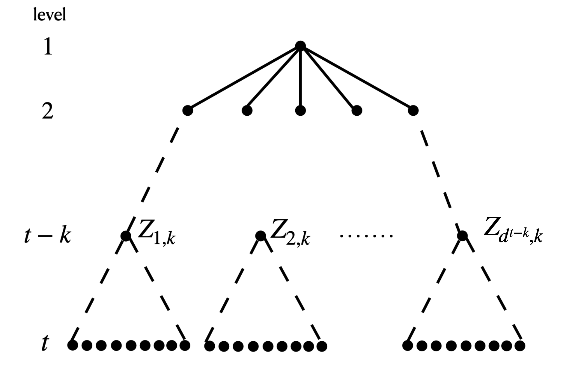
On the leaves of each of these subtrees, run the algorithm from Theorem 4.4 and suppose the outputs are beliefs () for the nodes at level of the broadcast tree. Now, recursively apply belief propagation until we reach the root and output the belief thus obtained. Specifically, recursively define
for and , where is the belief propagation function given by
We can restate Theorem 4.4 in terms of an upper bound on the maximum perturbation from the ground truth .
5 Information-theoretic lower bounds
First, we establish the folklore result that the -fraction adversary is very powerful and can in fact completely erode any information in the leaves about the posterior distribution of the root.
Definition 5.1.
Fix . The -fraction adversary is allowed to look at all the spins of the leaves and then flip the signs of leaves of his choosing.
Theorem 5.2.
For every , and , there exists some such that if the -fraction adversary is allowed to corrupt the leaves of the broadcast on tree process with parameters that was run up to level , it is information theoretically impossible to recover the root vertex. In fact, we prove that for there exists a -fraction adversary A for which we have
The quantitative bound in the theorem implies that it is impossible to have an algorithm A that recovers the root vertex with an advantage larger than .
Proof.
Set and throughout this proof we consider . Let be the distribution of the leaves at level of a broadcast process with parameters with root being and be the distribution with root being . And, let be the analogous joint distributions on the first levels of the broadcast tree.
We claim that it suffices to exhibit a coupling between and such that with probability , we have where refers to Hamming distance between the two strings.
Indeed, consider the following -fraction adversary : for , if then let , where by our choice of parameters we have that . Otherwise, let . Let denote the distribution corresponding to where . In particular, this means that
It suffices therefore to exhibit the coupling as claimed. Define for to act as follows: (in the following, let ) here one should think of marked vertices as the vertices where the adversary did not make any changes, and the goal of the adversary is to flip unmarked vertices that are labelled ‘+’ to ‘-’
-
•
Sample (that is, conditioned on the leaves of the tree taking labels ).
-
•
Let .
-
•
Traverse down the tree starting from the the nodes at level 1, that is, from the children of the root. If the current node is marked, let and mark all its children. Otherwise, if is unmarked and , then mark and all its children and set . Else, if is unmarked and , with probability leave it unmarked and set . Otherwise with probability , mark and its children and set .
-
•
Let be the restriction of to the vertices at level .
In order to prove that this coupling has the desired properties, we first show that with high probability, the Hamming distance between and is small.
Note that if for a vertex at the -th level, we have then has to be unmarked, and furthermore there is a path of unmarked vertices connecting to the root. The latter occurs with probability at most . Applying Markov’s inequality immediately gives
Next, we need to show that . We will actually show that by inducting on . For the base case, note that for any vertex on level 1, we have that
as desired.
For , we write to denote the restriction of to labels of vertices in levels . Note that it suffices to prove that for any vertex at level with parent ,
Indeed, note that
Since
and , the above indeed implies that
as desired. ∎
Another natural question is whether the bound on in Theorem 1.4 is tight; that is, can we prove any information theoretic lower bounds on -semi-random adversaries? To that end, we have the following upper bound of . This means that at least in the range of being a log-factor above the Kesten-Stigum threshold, belief propagation achieves the optimal (up to constant factors) in terms of being robust against -semi-random adversaries.
Theorem 5.3.
For every and , there exists such that if a -semi-random adversary is allowed to corrupt the leaves of the broadcast on tree process with parameters that was run up to level , then it is information theoretically impossible to recover the root vertex. That is, for there exists a -semi-random adversary A such that
Proof.
Set . We adapt the adversary that we used to prove the information theoretic bound in Theorem 5.2. Retain the notations as in the proof of Theorem 5.2, where defines a coupling on . Consider the following adversary B: for , if all the sites of (i.e. the sites where the two vectors differ) are selected as possible sites for corruption, and we call this event good, then output . Otherwise, return . Let denote the distribution corresponding to where .
We claim that the good event happens with probability . To that end, we traverse down the tree and mark vertices as in the process described in Theorem 5.2 until we reach level . For each of these marked vertices on level , we simulate the process of choosing whether to mark its children with the coin flips in the -semi-random adversary. In other words we couple random coin flips to mark the children and change their spins with the coin tosses in the adversary. The bound on the semi-random robust gain follows from Theorem 5.2 as well. ∎
Acknowledgements
We thank Guy Bresler and Po-Ling Loh for helpful conversations as this manuscript was being prepared.
Appendix A Deferred proofs
Proof of Corollary 1.6.
We claim that an equivalent formulation of Theorem 1.4 is that for any satisfying suitable hypothesis, there exists such that for any adversary B that takes as input and and is only allowed to flip the signs of the restriction , there exists an algorithm ALG with the following guarantee:
for all where is the uniform distribution on subsets of cardinality .
To this end, note that if then
Let be the distribution on subsets of cardinality where . Note that is decreasing on the range since . Consequently,
where the final inequality follows from the Chernoff bound. This implies that we can take .
By an application of Markov’s inequality, it follows that of subset have the property that
| (19) |
We claim that we can take to consist of the subsets which satisfy (19). First we check that these subsets have the desired property. Indeed, it suffices to note that for any with , we have
where the first inequality follows because of the convexity of the total variation distance and the second inequality follows by (19).
Finally, we show that is large in size. This follows because
where the second inequality is true for sufficiently large . ∎
Proof of Claim 3.5.
Let and . We claim that
The desired inequality then follows from the fundamental theorem of calculus. Now, and so when , we have and when we have . ∎
Proof of Claim 3.7.
It suffices to note that for sufficiently small , we have
Indeed, the above holds as for sufficiently small , we have
as desired. ∎
Proof of Claim 3.8.
It suffices to note that for
By setting and , it follows that for sufficiently small , it follows that the desired quantity is bounded above by a constant. ∎
Proof of Lemma 3.12.
In what follows, denote . We adapt the proof of [MNS16, Lemma 3.16]. For simplicity of notation denote . By applying Markov’s inequality to Lemma 3.10, it follows that for some to be chosen and sufficiently large relative to , we have
Since , it follows that
The remainder of the proof is near verbatim that of [MNS16, Lemma 3.16] and we repeat it here for completeness. Since is decreasing in , it follows that
for any random variable supported on and . Applying this for and , the above probability estimate implies that
We claim that we can make each of the terms above bounded away from by taking and . Note that this choice of satisfies .
We can compute
where the second inequality follows by Taylor expanding around , and our choice of parameters ensure that so that the derivative of is bounded. Finally, it can be checked that the above is bounded away from for our choice of parameters for our choice of and since ; in fact our choice of parameters ensures that for some . This follows because for , we have that and we also have and so we can write
We can also compute
Note that is bounded away from on the interval by our earlier calculation.
It follows that there is some such that for all , there is some such that
as desired. ∎
References
- [Abb18] Emmanuel Abbe. Community detection and stochastic block models: recent developments. Journal of Machine Learning Research, 18(177):1–86, 2018.
- [BB86] James Berger and L Mark Berliner. Robust bayes and empirical bayes analysis with -contaminated priors. The Annals of Statistics, pages 461–486, 1986.
- [BKMP05] Noam Berger, Claire Kenyon, Elchanan Mossel, and Yuval Peres. Glauber dynamics on trees and hyperbolic graphs. Probability Theory and Related Fields, 131(3):311–340, 2005.
- [BMR21] Jess Banks, Sidhanth Mohanty, and Prasad Raghavendra. Local statistics, semidefinite programming, and community detection. In Proceedings of the 2021 ACM-SIAM Symposium on Discrete Algorithms (SODA), pages 1298–1316. SIAM, 2021.
- [CKMY22] Sitan Chen, Frederic Koehler, Ankur Moitra, and Morris Yau. Kalman filtering with adversarial corruptions. In Proceedings of the 54th Annual ACM SIGACT Symposium on Theory of Computing, pages 832–845, 2022.
- [DdNS22] Jingqiu Ding, Tommaso d’Orsi, Rajai Nasser, and David Steurer. Robust recovery for stochastic block models. In 2021 IEEE 62nd Annual Symposium on Foundations of Computer Science (FOCS), pages 387–394. IEEE, 2022.
- [DGT19] Ilias Diakonikolas, Themis Gouleakis, and Christos Tzamos. Distribution-independent pac learning of halfspaces with massart noise. Advances in Neural Information Processing Systems, 32, 2019.
- [DK23] Ilias Diakonikolas and Daniel M Kane. Algorithmic High-dimensional Robust Statistics. Cambridge University Press, 2023.
- [DKTZ20] Ilias Diakonikolas, Vasilis Kontonis, Christos Tzamos, and Nikos Zarifis. Learning halfspaces with massart noise under structured distributions. In Conference on Learning Theory, pages 1486–1513. PMLR, 2020.
- [DMR06] Constantinos Daskalakis, Elchanan Mossel, and Sébastien Roch. Optimal phylogenetic reconstruction. In Proceedings of the thirty-eighth annual ACM symposium on Theory of computing, pages 159–168, 2006.
- [EKPS00] William Evans, Claire Kenyon, Yuval Peres, and Leonard J Schulman. Broadcasting on trees and the ising model. Annals of Applied Probability, pages 410–433, 2000.
- [Goo50] Isidore Jacob Good. Probability and the Weighing of Evidence. Charles Griffin & Co., Ltd., London; Hafner Publishing Co., New York, 1950.
- [IS23] Misha Ivkov and Tselil Schramm. Semidefinite programs simulate approximate message passing robustly. arXiv preprint arXiv:2311.09017, 2023.
- [JM04] Svante Janson and Elchanan Mossel. Robust reconstruction on trees is determined by the second eigenvalue. Ann. Probab., 32(3B):2630–2649, 2004.
- [Kea90] Michael J Kearns. The computational complexity of machine learning. MIT press, 1990.
- [LM22] Allen Liu and Ankur Moitra. Minimax rates for robust community detection. In 2022 IEEE 63rd Annual Symposium on Foundations of Computer Science (FOCS), pages 823–831. IEEE, 2022.
- [MN06] Pascal Massart and Élodie Nédélec. Risk bounds for statistical learning. Ann. Statist., 34(5):2326–2366, 2006.
- [MNS15] Elchanan Mossel, Joe Neeman, and Allan Sly. Reconstruction and estimation in the planted partition model. Probability Theory and Related Fields, 162:431–461, 2015.
- [MNS16] Elchanan Mossel, Joe Neeman, and Allan Sly. Belief propagation, robust reconstruction and optimal recovery of block models. Ann. Appl. Probab., 26(4):2211–2256, 2016.
- [Mos04] Elchanan Mossel. Survey: Information flow on trees. arXiv preprint math/0406446, 2004.
- [MPW16] Ankur Moitra, William Perry, and Alexander S. Wein. How robust are reconstruction thresholds for community detection? In STOC’16—Proceedings of the 48th Annual ACM SIGACT Symposium on Theory of Computing, pages 828–841. ACM, New York, 2016.
- [MSW04] Fabio Martinelli, Alistair Sinclair, and Dror Weitz. Glauber dynamics on trees: boundary conditions and mixing time. Communications in Mathematical Physics, 250:301–334, 2004.
- [Pol23] Yury Polyanskiy. Personal communication, December 2023. Personal communication with Yury Polyanskiy.
- [YP22] Qian Yu and Yury Polyanskiy. Ising model on locally tree-like graphs: Uniqueness of solutions to cavity equations. arXiv preprint arXiv:2211.15242, 2022.