Parameter & Data Efficient Spectral Style-DCGAN

Abstract

We present a simple, highly parameter, and data-efficient adversarial network for unconditional face generation. Our method: Spectral Style-DCGAN or SSD utilizes only 6.574 million parameters and 4739 dog faces from the Animal Faces HQ (AFHQ) (Choi et al., 2020) dataset as training samples while preserving fidelity at low resolutions up to 64x64. Code available at Github.

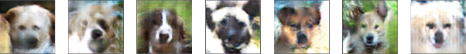
Figure 1: Spectral normalized discriminator improvement synthesis

1 Introduction

Typically, modern high-fidelity generators need $\sim$ $10^{5}-10^{6}$ images, which makes training GANs extremely costly and disadvantages important sectors like medicine (Yi et al., 2019). DCGAN (Radford et al., 2016) the first and arguably the smallest convolutional GAN (Goodfellow et al., 2014) still required tremendous amounts of training data: LSUN (Yu et al., 2015) ($\sim$3 million) and ImageNet-1K (Russakovsky et al., 2015) ($\sim$1.28 million). Data-efficient GAN frameworks that utilize tiny datasets of sizes $\sim 10^{3}$ are often marred with extensive compute requirements and/or massive parameterization (Tran et al., 2021; Lu et al., 2023; Karras et al., 2020b). See A.2. To alleviate the high data and parameters, we make the following contributions: a) We contribute a robust GAN framework that utilizes tiny datasets ($\sim$5000 samples), comparable to (Karras et al., 2020b; Kumari et al., 2022) while being extremely parameter-efficient. At 6.57 million parameters we use 624.44% fewer parameters than the state-of-the-art StyleGAN and variants. b) We demonstrate for the first time how spectral normalization implicitly aids meaningful generator-side learning and latent space disentanglement.

2 Method

To effectively understand the distribution and consequently not overfit, the generator needs to learn diverse image contents(pose, identity) and styles(hair, eye color). Gatys (Gatys et al., 2016) show that style and content are separable. Furthermore, sufficient disentanglement in the stochastic style space is needed for the generator to localize the style to the relevant content or regions of the image. Inspired by StyleGAN’s (Karras et al., 2019) learned style constant and adaptive instance normalization (adaIN) (Huang & Belongie, 2017a) to enforce the style, our generator’s head is a tiny 100-dimensional 4-layer MLP head, unlike StyleGAN-2’s huge 512-dimensional 8-layer MLP. This head maps the noise to a disentangled style-space similar to Karras et al. (2019; 2020b). The learned style vector is used for adaIN layers (Huang & Belongie, 2017b) introduced in our custom-DCGAN’s deconvolutional upsampling generator block. Finally, the synthesized and real images are sent to a spectrally normalized (SN) Miyato et al. (2018) weights’ ($W_{SN}:=W/\sigma(W)$) custom-DCGAN discriminator. This discriminator choice is inspired by the key insights from Arjovsky & Bottou (2017); Zhang & Khoreva (2019); Karras et al. (2020a) that the discriminator overfits in low data regimes to the training examples subsequently making the feedback to the generator meaningless. This diverges the overall training. To avoid vanishing gradients and increasing the parameters significantly we choose spectral normalization as an internal regularizer for the discriminator. Overall, these potent improvements allow our method to be data and parameter-efficient. Refer to Appendix A.5 for more architectural details.

3 Experiments

3.1 Results & Spectral Normalization Ablation

We observe that SN discriminator improvement slows the discriminator (Fig. 4) down thus allowing the generator to learn meaningful and coherent faces. See Fig 1. Without the SN improvement, the generator is not able to learn better high-level facial attributes like head shape, number of ears, etc. as shown in the ablation Fig 2.

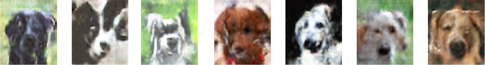
Figure 2: Ablation: No spectral normalization. Style Mapping and AdaIN synthesis

3.2 Quantitative Comparison & Data-Efficiency Ablation

We quantitatively evaluate our method, DCGAN (Radford et al., 2016) and StyleGAN (Karras et al., 2019) under identical deterministic settings using FID (Heusel et al., 2018a) in Table 1. We trained all baselines and our method for 20 epochs on the AFHQ Dog Subset with default hyperparameters.

Method	Parameters (M)	FID $\downarrow$
DCGAN (Radford et al., 2016)	6.342	424.512
StyleGAN (Karras et al., 2019)	47.625	355.620
Ours	6.574	285.579

Table 1: Generation fidelity and parameters: Our method produces the highest-fidelity results and uses 624.44% fewer parameters compared to StyleGAN. We also observe that StyleGAN requires significantly more data ($\sim 5\times 10^{4}$ images) and intensive training time to match our fidelity score.

To further validate our data-efficient solution, we perform ablation in Table 2 and evaluate the generation fidelity. Due to the aliased resizing operation, we observe an inconsistency in PyTorch-FID scores, similar to (Parmar et al., 2022). So, we evaluate further using clean-FID (Parmar et al., 2022) and clean-Kernel Inception Distance (Bińkowski et al., 2021; Parmar et al., 2022)

Training Data ($K$%)	FID $\downarrow$	clean-FID $\downarrow$	clean-KID $\downarrow$
100%	285.579	274.139	0.2054
75%	241.581	283.536	0.2379
50%	294.467	293.038	0.2452
25%	319.899	319.241	0.2510

Table 2: Ablation: Data Efficiency. Using $K$% of the dogs-AFHQ training split, we estimate the generation quality using FID, clean-FID (Parmar et al., 2022) and clean Kernel Inception Distance (Bińkowski et al., 2021) (clean-KID)

URM Statement

The authors acknowledge that the author of this work meets the URM criteria of the ICLR 2024 Tiny Papers Track.

Appendix A Appendix

The code is available at: repo.

A.1 Important note on the FID scores

FID scores are high as we upsampled the generated images while downsampling the real distribution from 512x512 due to compute limitations. Additionally, the 2048th layer of InceptionV3 is used to compute FID.

We notice the counter-intuitive dip in FID when using only 75% data in Tab. 2 and pin-point the issue to large aliasing during resizing operations done internally by PyTorch-FID, as first observed in (Parmar et al., 2022). So, we decide to use the clean-FID and clean-KID metrics from (Parmar et al., 2022) as well for Tab. 2.

The StyleDCGAN notebook in our codebase has the output cells saved as well with the clean-FID metrics for verification.

A.2 Extended Introduction/Motivation

With the substantial fidelity gains of GANs Goodfellow et al. (2014) over other explicit density modeling methods including VAEs (Kingma & Welling, 2022), many ground-breaking applications in defense (Bistron & Piotrowski, 2021), engineering (Luleci et al., 2022), healthcare (Yi et al., 2019) have made GANs mainstream.

GANs are being succeeded by diffusion and Poisson generative models (Croitoru et al., 2023) but still are extremely valuable as they use significantly less compute while still staying competitive in terms of fidelity (Dhariwal & Nichol, 2021).

However, modern GANs still require massive (of the order of $10^{6}$) training datasets (Karras et al., 2020a), and are often parametrically overburdened. For instance, StyleGAN-XL (Sauer et al., 2022) used $3\times$ more parameters than StyleGAN3 (Karras et al., 2021) and consumed massive amounts of energy during training. The environmental impact of StyleGAN3 was 224.62 Mega Watt Hours(MWh) and 91.77 GPU years or the time it would take one NVIDIA V100 to train. To put the energy impact in perspective, an average American citizen uses a total of 12.71 MWh in a year (data from EIA report, 2022).

This significantly limits the usage of GANs to a select few. When small GANs (networks’ parameters) and low-data regimes($\sim 10^{3}$) are used, detrimental issues like overfitting, mode collapse, aggravated loss divergence due to the inherent instability in the adversarial training set-up and significantly reduced generation fidelity are observed (Li et al., 2022). This is a critical issue for deployment and crucial applications. Especially in the healthcare sector, which is plagued by a chronic scarcity of labeled data (Yi et al., 2019).

To alleviate these pressing issues and still retain the advantages of this valuable technology, we present a parameter and data-efficient GAN that also trains quickly and stably.

A.3 Related Works

Strategy	Methods
Data Augmentation	Differential Augmentation (Zhao et al., 2020),
	GANs for synthetic data (Figueira & Vaz, 2022)
Loss side	WGAN (Arjovsky et al., 2017), Vision-Aided GAN Kumari et al. (2022)
	WGAN-GP, RaGAN (Jolicoeur-Martineau, 2018)
Training Regimes	TTUR (Heusel et al., 2018b)
Network Side	StyleGAN2-ADA (Karras et al., 2020a), Ours

Table 3: Related Works: In this table, we present noteworthy works for increasing data-efficiency(DE), parameter-efficiency(PE), and overall training stability(TS) of GANs

A.4 Dataset

We choose the dogs’ subset of the AFQH (Choi et al., 2020) dataset and use the default StarGAN-v2 split where 4739 are training samples while 500 are reserved for validation. We use PyTorch’s default bilinear interpolation to downsample all images to 64x64 from the original 512x512 resolution, for training and validation.

Figure 3: Training dataset samples at original 512x512 resolution.

A.5 Architecture & Training Details

A.5.1 Generator

The Generator takes in a 100-dimensional noise vector ($Z$-space) and then is mapped to another 100-dimensional vector ($W$-space) using a custom MLP named: MappingNetwork. This transformed vector aids in the disentanglement of the feature space and acts as a style vector used for computations for the adaptive instance normalization layers in the generator. Nevertheless, the MappingNetwork consists of 4 linear layers (same input-output dimensionality), each followed by an in-place leaky-ReLU activation with a slope of 0.2.

Following this simple mapping, we move towards a custom DCGAN where each fractionally strided convolution or transposed convolution is followed by an adaptive instance normalization (Huang & Belongie, 2017a) (just like StyleGAN) and finally a ReLU activation. The adaptive instance normalization layer repeatedly uses the W-space transformed latent to learn an affine transformation for the already instance normed output of the transposed-convolution layer. Simply put, $AdaIN(x_{i},w)=\alpha(w)*\frac{(x_{i}-\mu_{i})}{\sqrt{\sigma^{2}_{i}+\epsilon}}+\beta(w)$ where $\alpha$ and $\beta$ denote learnable linear layers.

The last and the 5th transposed convolution layer is special as it does not have an adaptive instance normalization layer and is succeeded by a TanH activation layer. These changes mark a significant deviation in the generator from both StyleGAN (Karras et al., 2019) and DCGAN (Radford et al., 2016).

The generator contains a total of 3,809,104 parameters and is trained with an Adam (Kingma & Ba, 2017) optimizer with a learning rate of $0.0005$ and $\beta_{1}$ of $0.5$ and $\beta_{2}$ equal to $0.999$.

A.5.2 Discriminator

Our discriminator is a tiny (2,765,568 parameters) 5-convolution layer CNN that uses spectral normalization followed by standard batch normalization and in-place Leaky-ReLU with default PyTorch parameters. This orthogonal combination of spectral normalization and then batch normalization layers provides enough regularization for stable adversarial training with the Adam (Kingma & Ba, 2017) optimizer. The learning rate is $0.0005$ and $\beta_{1}$ is set to $0.5$ while $\beta_{2}$ equals $0.999$.

A.5.3 Alternate Steps, Criterion & Framework

For every generator step, we move the discriminator one step as well. We only use the binary cross-entropy or adversarial criterion ($L_{a}dv(y_{i},x_{i})$ = $y_{i}*log(x_{i})+(1-y_{i})*log(1-x_{i})$; $y_{i}\in\{0,1\}$) for our unconditional generative solution. We monitor the generator’s validation loss and save the best one. We use PyTorch-Lightning for abstraction and a free Google Colab P100-GPU session for 20 epochs of training with a batch size of 32.

Please refer to the notebook version of our implementation in repo for a detailed architecture summary, training parameters, and more details.

A.6 Further Experiments

A.6.1 Ablation: With and without spectral normalization training losses

We argue that the weight regularization or spectral normalization slows down the discriminator allowing the generator to learn a richer and more diverse distribution. This slow learning for the generator is essential to avoid mode-collapse and diversity issues. Our argument is validated by the ablation in Fig. 4

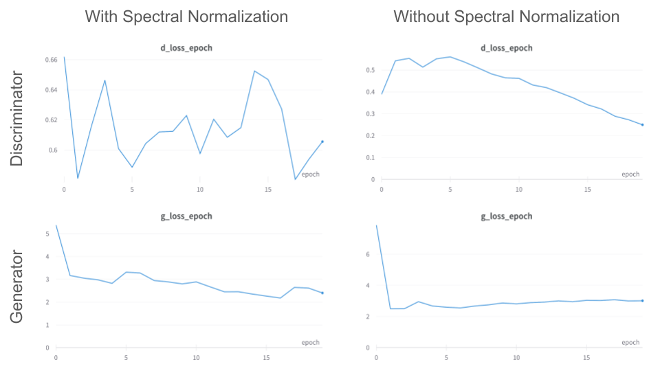
Figure 4: Ablation study: Effect of spectral normalization layers in the discriminator. The left column represents training loss plots of the discriminator(top) and generator(bottom) with the spectral normalization layers in the discriminator; while the right column demonstrates the ablated-discriminator-training loss plots.

A.6.2 Ablation: Style-Mapping Network Only Results (No AdaIN)

Here we see that disentanglement is not enough. We additionally need to repetitively fuse the learned style vector to get consistent textures, hair, and facial features and remove the aberrations. This is essential to fix the known problem that the latent space is always continuous, however, the real dataset is always discrete and discontinuous.

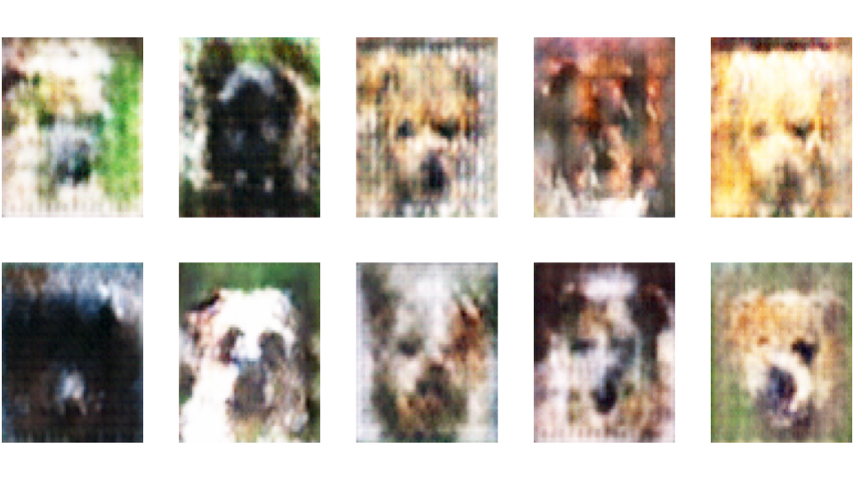
Figure 5: Ablation: Disentangling the latent vectors. Style-Mapping without AdaIN Synthesis

A.7 More Qualitative Results for Ablation: Without Spectral Normalization

We demonstrate some additional results of the ablation presented in Fig.2.

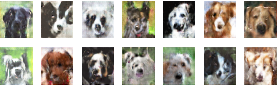
Figure 6: More Results of the ablation: No spectral normalization. Style Mapping and AdaIN synthesis

A.8 Z-Space Interpolation

We find a feature-preserving direction in our generator and linearly interpolate between two vectors sampled from this space. See 7.

(a) $z_{1}$

(b)

(c)

(d) $z_{2}$

Figure 7: Z-space Interpolation. We manually find a direction along which the ears are preserved. All dogs have just the left ear standing tall in (a) - (d).

A.9 Conclusion

We present a highly parameter and data-efficient GAN framework inspired by the seminal works: DCGAN and StyleGAN; getting the best of both worlds and further regularizing it with spectral normalization to learn meaningful and coherent underlying data distributions. Our work faces the limitation of not being able to impose any facial priors like lateral symmetry, pose, and feature positioning on the unconditional generation. Attention layers, as proposed in SAGAN (Zhang et al., 2019), can alleviate the same and aid in higher color consistency across the output image. However, this comes at an additional computational cost.

References

- Arjovsky & Bottou (2017) Martin Arjovsky and Léon Bottou. Towards principled methods for training generative adversarial networks, 2017.
- Arjovsky et al. (2017) Martin Arjovsky, Soumith Chintala, and Léon Bottou. Wasserstein gan, 2017.
- Bistron & Piotrowski (2021) Marta Bistron and Zbigniew Piotrowski. Artificial intelligence applications in military systems and their influence on sense of security of citizens. Electronics, 10(7), 2021. ISSN 2079-9292. doi: 10.3390/electronics10070871. URL https://www.mdpi.com/2079-9292/10/7/871.
- Bińkowski et al. (2021) Mikołaj Bińkowski, Danica J. Sutherland, Michael Arbel, and Arthur Gretton. Demystifying mmd gans, 2021.
- Choi et al. (2020) Yunjey Choi, Youngjung Uh, Jaejun Yoo, and Jung-Woo Ha. Stargan v2: Diverse image synthesis for multiple domains. In Proceedings of the IEEE Conference on Computer Vision and Pattern Recognition, 2020.
- Croitoru et al. (2023) Florinel-Alin Croitoru, Vlad Hondru, Radu Tudor Ionescu, and Mubarak Shah. Diffusion models in vision: A survey. IEEE Transactions on Pattern Analysis and Machine Intelligence, 45(9):10850–10869, 2023. doi: 10.1109/TPAMI.2023.3261988.
- Dhariwal & Nichol (2021) Prafulla Dhariwal and Alex Nichol. Diffusion models beat gans on image synthesis, 2021.
- Figueira & Vaz (2022) Alvaro Figueira and Bruno Vaz. Survey on synthetic data generation, evaluation methods and gans. Mathematics, 10(15), 2022. ISSN 2227-7390. doi: 10.3390/math10152733. URL https://www.mdpi.com/2227-7390/10/15/2733.
- Gatys et al. (2016) Leon A. Gatys, Alexander S. Ecker, and Matthias Bethge. Image style transfer using convolutional neural networks. In 2016 IEEE Conference on Computer Vision and Pattern Recognition (CVPR), pp. 2414–2423, 2016. doi: 10.1109/CVPR.2016.265.
- Goodfellow et al. (2014) Ian J. Goodfellow, Jean Pouget-Abadie, Mehdi Mirza, Bing Xu, David Warde-Farley, Sherjil Ozair, Aaron Courville, and Yoshua Bengio. Generative adversarial networks, 2014.
- Heusel et al. (2018a) Martin Heusel, Hubert Ramsauer, Thomas Unterthiner, Bernhard Nessler, and Sepp Hochreiter. Gans trained by a two time-scale update rule converge to a local nash equilibrium, 2018a.
- Heusel et al. (2018b) Martin Heusel, Hubert Ramsauer, Thomas Unterthiner, Bernhard Nessler, and Sepp Hochreiter. Gans trained by a two time-scale update rule converge to a local nash equilibrium, 2018b.
- Huang & Belongie (2017a) Xun Huang and Serge Belongie. Arbitrary style transfer in real-time with adaptive instance normalization, 2017a.
- Huang & Belongie (2017b) Xun Huang and Serge Belongie. Arbitrary style transfer in real-time with adaptive instance normalization, 2017b.
- Jolicoeur-Martineau (2018) Alexia Jolicoeur-Martineau. The relativistic discriminator: a key element missing from standard gan, 2018.
- Karras et al. (2019) Tero Karras, Samuli Laine, and Timo Aila. A style-based generator architecture for generative adversarial networks, 2019.
- Karras et al. (2020a) Tero Karras, Miika Aittala, Janne Hellsten, Samuli Laine, Jaakko Lehtinen, and Timo Aila. Training generative adversarial networks with limited data. In Proc. NeurIPS, 2020a.
- Karras et al. (2020b) Tero Karras, Samuli Laine, Miika Aittala, Janne Hellsten, Jaakko Lehtinen, and Timo Aila. Analyzing and improving the image quality of stylegan, 2020b.
- Karras et al. (2021) Tero Karras, Miika Aittala, Samuli Laine, Erik Härkönen, Janne Hellsten, Jaakko Lehtinen, and Timo Aila. Alias-free generative adversarial networks. In Proc. NeurIPS, 2021.
- Kingma & Ba (2017) Diederik P. Kingma and Jimmy Ba. Adam: A method for stochastic optimization, 2017.
- Kingma & Welling (2022) Diederik P Kingma and Max Welling. Auto-encoding variational bayes, 2022.
- Kumari et al. (2022) Nupur Kumari, Richard Zhang, Eli Shechtman, and Jun-Yan Zhu. Ensembling off-the-shelf models for gan training. In Proceedings of the IEEE/CVF Conference on Computer Vision and Pattern Recognition (CVPR), June 2022.
- Li et al. (2022) Ziqiang Li, Beihao Xia, Jing Zhang, Chaoyue Wang, and Bin Li. A comprehensive survey on data-efficient gans in image generation, 2022.
- Lu et al. (2023) Yingzhou Lu, Minjie Shen, Huazheng Wang, Capucine van Rechem, and Wenqi Wei. Machine learning for synthetic data generation: A review, 2023.
- Luleci et al. (2022) Furkan Luleci, F. Necati Catbas, and Onur Avci. A literature review: Generative adversarial networks for civil structural health monitoring. Frontiers in Built Environment, 8, 2022. ISSN 2297-3362. doi: 10.3389/fbuil.2022.1027379. URL https://www.frontiersin.org/articles/10.3389/fbuil.2022.1027379.
- Miyato et al. (2018) Takeru Miyato, Toshiki Kataoka, Masanori Koyama, and Yuichi Yoshida. Spectral normalization for generative adversarial networks, 2018.
- Parmar et al. (2022) Gaurav Parmar, Richard Zhang, and Jun-Yan Zhu. On aliased resizing and surprising subtleties in gan evaluation. In CVPR, 2022.
- Radford et al. (2016) Alec Radford, Luke Metz, and Soumith Chintala. Unsupervised representation learning with deep convolutional generative adversarial networks, 2016.
- Russakovsky et al. (2015) Olga Russakovsky, Jia Deng, Hao Su, Jonathan Krause, Sanjeev Satheesh, Sean Ma, Zhiheng Huang, Andrej Karpathy, Aditya Khosla, Michael Bernstein, Alexander C. Berg, and Li Fei-Fei. ImageNet Large Scale Visual Recognition Challenge. International Journal of Computer Vision (IJCV), 115(3):211–252, 2015. doi: 10.1007/s11263-015-0816-y.
- Sauer et al. (2022) Axel Sauer, Katja Schwarz, and Andreas Geiger. Stylegan-xl: Scaling stylegan to large diverse datasets, 2022.
- Tran et al. (2021) Ngoc-Trung Tran, Viet-Hung Tran, Ngoc-Bao Nguyen, Trung-Kien Nguyen, and Ngai-Man Cheung. On data augmentation for gan training. IEEE Transactions on Image Processing, 30:1882–1897, 2021. ISSN 1941-0042. doi: 10.1109/tip.2021.3049346. URL http://dx.doi.org/10.1109/TIP.2021.3049346.
- Yi et al. (2019) Xin Yi, Ekta Walia, and Paul Babyn. Generative adversarial network in medical imaging: A review. Medical Image Analysis, 58:101552, 2019. ISSN 1361-8415. doi: https://doi.org/10.1016/j.media.2019.101552. URL https://www.sciencedirect.com/science/article/pii/S1361841518308430.
- Yu et al. (2015) Fisher Yu, Yinda Zhang, Shuran Song, Ari Seff, and Jianxiong Xiao. Lsun: Construction of a large-scale image dataset using deep learning with humans in the loop. arXiv preprint arXiv:1506.03365, 2015.
- Zhang & Khoreva (2019) Dan Zhang and Anna Khoreva. Progressive augmentation of gans, 2019.
- Zhang et al. (2019) Han Zhang, Ian Goodfellow, Dimitris Metaxas, and Augustus Odena. Self-attention generative adversarial networks, 2019.
- Zhao et al. (2020) Shengyu Zhao, Zhijian Liu, Ji Lin, Jun-Yan Zhu, and Song Han. Differentiable augmentation for data-efficient gan training, 2020.