New method for the solution of the two-body Dirac equation: Estimation of the weights of $C$, $P$ and $CP$ symmetry-violating terms in positronium

Abstract

A new theoretical method is developed for the solution of the two-body bound-state Dirac equation for positronium. Only Coulomb potential was included in the Dirac Hamiltonian. It is shown that the two-body Dirac Hamiltonian can be written in the Hermitian matrix form of the $4\times 4$ size and contains terms, responsible for the violation of the $P$, $C$, and $CP$ symmetries. Numerical results for the energy spectrum of the para- and ortho-positronium ground states performed within the variational method using the harmonic oscillator basis functions are in good agreement with a high-precision finite-element method of T.C. Scott et al. The weights of the $P$ and $CP$ symmetry-violating components in the para-positronium ground state are identical to the weight of the $P$ symmetry-violating component of the ortho-Ps and are estimated to be 6.6E-6. The weights of the $C$ and $CP$ symmetry-violating components of the ortho-Ps are equal to the 2/3 and 1/3 parts of this value, respectively. These numbers are less by two orders of magnitude than the accuracy limit of current experimental facilities.

I Introduction

A new generation of the high sensitivity and multi-photon total-body positron emission tomography systems opens perspectives for clinical applications of positronium (Ps) in medicine bas2023 . On the other hand, Ps is the most important object for the precision tests of the violation of the discrete symmetries such as C (charge conjugation), P (spatial parity), T (time reversal) and their combinations PhysRep2022 . The spin-singlet bound states of the electron $e^{-}$ and its antiparticle, the positron $e^{+}$ present para-positronium ($p$-Ps), at the same time the spin-triplet bound states present the ortho-positronium (o-Ps). If the bound (para- or ortho-) positronium is in the state with orbital momentum $\ell$, then its $P$ symmetry is defined by the phase factor $(-1)^{\ell+1}$ including the intrinsic opposite parities of the $e^{-}$ and $e^{+}$. Consequently, the $C$ symmetry is defined by the eigenvalue $(-1)^{\ell+S}$ of the charge-conjugation operator which is obtained from the request of antisymmetry of the total wave function as a product of the spatial and spin wave functions. Then for the resulting eigenvalue of the $CP$ symmetry operator one obtains $(-1)^{S+1}$. Without violation of one of the discrete symmetries these phase factors should be conserved.

On the other hand, the search of the violation of the $CP$ symmetry concerns a very fundamental problem of the dominance of the matter over the anti-matter. The main question is, are the matter and anti-matter abundances different from the beginning? The answer to this question may reveal the mystery of the matter-dominated Universe. According to the Big Bang theory, the initial amounts of matter and anti-matter were equal. When matter and anti-matter come into contact, they annihilate into pure photons and nothing else. If so, how can be explained that some amount of matter survive the primordial annihilation? In 1967, Andrei Sakharov proposed a solution to this puzzle sakh1967 . Sakharov’s explanation required the violation of the fundamental symmetry of Nature, the $CP$ symmetry. In 1964 the $CP$ symmetry violation was discovered by Val Fitch and Jim Cronin, and collaborators for the first time chris1964 in the study of the decays of neutral $K$-mesons (kaons). The $CP$ violation in kaons was later explained by Makoto Kobayashi and Toshihide Maskawa by postulating the existence of a third family of quarks, the strange ($S$) quarks kob1973 . However, the amount of baryons in the Universe predicted within the Standard Model using the Kobayashi-Maskawa mechanism falls several orders of magnitude smaller than what is observed by astronomers yam2010 . The question is, whether the Standard Model is able to indicate other sources of $CP$ violation or new physics beyond the Standard Model is required rub2004 . In the meantime, a possible source of the $CP$ violation could be hidden in the structure of positronium PhysRep2022 .

There are several experimental research groups involved in the search for CP violation in ortho-positronium decay bar2020 ; hau2023 . The photon has intrinsic odd $C$ parity, and consequently the n-photon state has charge-conjugation parity $C_{\gamma}=(-1)^{n}$. The $C$ symmetry conservation requires a selection rule for annihilation of the positronium state with the orbital momentum $\ell$ and spin $S$ into n-photon state: $(-1)^{\ell+S}=(-1)^{n}$. The experimental tests for $C$ symmetry violation in Ps search for decays to the wrong ($C$ forbidden) numbers of photons. The dominant decay mode of para-Ps is two-photon decay, while for ortho-Ps it is three-photon decay. In Ref. vet2002 no $C$ (charge-conjugation) symmetry violating events were observed in the positronium decay to four- and five-photon final states. Recent experimental study of the $P$, $T$, and $CP$ symmetry violation tests using linear polarization of photons from ortho-positronium annihilations did not show evidence of the violations of above symmetries at $10^{-4}$ precision NatCom2024 . These tests confirm results of previous $CP$ violation search in the ortho-positronium decay with a sensitivity of $2.2\times 10^{-3}$ yam2010 . The preference for the symmetry violating checks in $o$-Ps is connected with its longer 142 ns life-time in comparison with a small 1.25$\times 10^{-10}$ s life-time of the $p$-Ps.

While the experimental groups are working on increasing the precision of the experimental data bar2020 ; hau2023 ; vet2002 ; NatCom2024 ; yam2010 for the $CP$ violation tests in positronium, any prediction within theoretical models would help to solve the problem. A possible theoretical estimate of the precision needed for the discrete symmetry violation search would be very useful for the experimental setup. The most important spectroscopic properties of the positronium, such as energy-level intervals are reproduced with a high precision at order $\alpha^{6}$ within the non-relativistic QED PR13 ; PR25 ; PR125 ; PR126 ; PR242 based on the solutions of the Schrödinger bound-state equation. The explicit relativistic invariance built into QED is essential for particle physics but leads to unnecessary complications when QED is applied to Coulombic bound states, which deals with the energy scales small compared to $m_{e}c^{2}$ PhysRep2022 . On the other hand, relativistic theory could help to resolve problems, connected with the above $CP$ violation search in positronium. The two-body Dirac equation (TBDE) for positronium was studied in Ref. scott1992 using only the Coulomb interaction potential. In Ref.fer2023 the sixteen-component, no-pair Dirac-Coulomb-Breit equation, derived from the Bethe-Salpeter equation, is solved in a variational procedure using Gaussian-type basis functions for positronium, muonium, hydrogen atom, and muonic hydrogen. Recent studies of properties of anomalous bound states within the TBDE formalism pat19 ; pat23 have demonstrated that there are still many open questions for the structure of positronium. Another type of relativistic Schrödinger equation was obtained and solved based on the Pauli reduction of the TBDE cra2006 ; cra2009 .

The aim of present work is to study the two-body Dirac equation in details from the viewpoint of the $CP$ violation search in positronium. We solve the TBDE for the positronium bound states within a new theoretical method. The method is based on the Hermitian Dirac Hamiltonian in the form of $4\times 4$ matrix, each element of which represents a four-component operator. The solution of the TBDE for the positronium state with total momentum $J$ and its projection $M$ with the spin-orbital couplings $\vec{\mathbf{J}}=\vec{\mathbf{l}}+\vec{\mathbf{S}}$ and $\vec{\mathbf{S}}=\vec{\mathbf{S}}_{1}+\vec{\mathbf{S}}_{2}$, $S_{1}=S_{2}=1/2$, can be expressed in the form of a column of four components. Each of the large-large (LL), large-small (LS), small-large (SL) and small-small (SS) components of the eigen function represents a four-component spinor. The radial parts of these components are expressed as linear combination of the basic functions. The main advantage of the method is that this form of the Hermitian Dirac Hamiltonian contains a term $\vec{\boldsymbol{\sigma}}\hat{\vec{\mathbf{p}}}$, responsible for the violation of the $C$, $P$ and $CP$ symmetries. Numerical calculations have been performed within the variational method on the harmonic oscillator basic functions gutsche ; gutschedis ; tur09 ; tur14 .

In Section II we give the main formalism of the method. Section III deals with numerical results and the conclusions are presented in the last Section.

II Solution of the two-body bound state Dirac equation

II.1 Two-body Dirac equation for positronium bound states

The Dirac Hamiltonian for the two-body bound system interacting via Coulomb potential ($\hbar=c=1$) is written in the form scott1992

$$\hat{\mathbf{H}}=\vec{\boldsymbol{\alpha}}_{1}\times\mathbf{I}^{(2)}_{4}\cdot\vec{\mathbf{p}}_{1}+\mathbf{I}^{(1)}_{4}\times\vec{\boldsymbol{\alpha}}_{2}\cdot\vec{\mathbf{p}}_{2}+\beta_{1}\times\mathbf{I}^{(2)}_{4}m_{1}+\mathbf{I}^{(1)}_{4}\times\beta_{2}m_{2}+\mathbf{I}_{16}{V}(r_{12}),$$ (1)

where the Dirac matrices

$$\vec{\boldsymbol{\alpha}}=\beta\vec{\boldsymbol{\gamma}}=\begin{pmatrix}0&\vec{\boldsymbol{\sigma}}\\ \vec{\boldsymbol{\sigma}}&0\end{pmatrix},\qquad\beta=\gamma^{0}=\begin{pmatrix}\mathbf{I}_{2}&0\\ 0&-\mathbf{I}_{2}\end{pmatrix},$$ (2)

and $\mathbf{I}_{n}$ is the unit $n\times n$ matrix operator, ${V}(r_{12})$ is the Coulomb potential. Index 1 (2) of the operator means that this operator acts on the wave function of the first (second) particle. In order to write the Hamiltonian in the relative coordinates we introduce the radius-vectors of the center of mass $\vec{\mathbf{R}}$ and the relative-motion $\vec{\mathbf{r}}$ of the positron-electron two-body system:

$$\begin{array}[]{l}\vec{\mathbf{R}}=\dfrac{1}{2}(\vec{\mathbf{r}}_{1}+\vec{\mathbf{r}}_{2}),\quad\vec{\mathbf{r}}=\vec{\mathbf{r}}_{1}-\vec{\mathbf{r}}_{2}.\end{array}$$

With the assumption $\vec{\mathbf{P}}_{\mathbf{R}}=0$, one can write the total Dirac Hamiltonian of the relative motion in terms of the relative momentum $\vec{\mathbf{p}}$ and coordinate $\vec{\mathbf{r}}$:

$$\begin{array}[]{l}\hat{\mathbf{H}}=\left\{\vec{\boldsymbol{\alpha}}_{1}\times\mathbf{I}^{(2)}_{4}-\mathbf{I}^{(1)}_{4}\times\vec{\boldsymbol{\alpha}}_{2}\right\}\cdot\vec{\mathbf{p}}+\beta_{1}\times\mathbf{I}^{(2)}_{4}m_{1}+\mathbf{I}^{(1)}_{4}\times\beta_{2}m_{2}+\mathbf{I}_{16}{V}(r).\end{array}$$ (3)

Using the standard representation of Dirac gamma matrices, the kinetic part of the Hamiltonian can be written in the form of symmetric matrix:

$$\left\{\vec{\boldsymbol{\alpha}}_{1}\times\mathbf{I}^{(2)}_{4}-\mathbf{I}^{(1)}_{4}\times\vec{\boldsymbol{\alpha}}_{2}\right\}\cdot\vec{\mathbf{p}}=\begin{pmatrix}0&-\mathbf{I}^{(1)}_{2}\times\vec{\boldsymbol{\sigma}}_{2}\cdot\vec{\mathbf{p}}&\vec{\boldsymbol{\sigma}}_{1}\times\mathbf{I}^{(2)}_{2}\cdot\vec{\mathbf{p}}&0\\ \\ -\mathbf{I}^{(1)}_{2}\times\vec{\boldsymbol{\sigma}}_{2}\cdot\vec{\mathbf{p}}&0&0&\vec{\boldsymbol{\sigma}}_{1}\times\mathbf{I}^{(2)}_{2}\cdot\vec{\mathbf{p}}\\ \\ \vec{\boldsymbol{\sigma}}_{1}\times\mathbf{I}^{(2)}_{2}\cdot\vec{\mathbf{p}}&0&0&-\mathbf{I}^{(1)}_{2}\times\vec{\boldsymbol{\sigma}}_{2}\cdot\vec{\mathbf{p}}\\ \\ 0&\vec{\boldsymbol{\sigma}}_{1}\times\mathbf{I}^{(2)}_{2}\cdot\vec{\mathbf{p}}&-\mathbf{I}^{(1)}_{2}\times\vec{\boldsymbol{\sigma}}_{2}\cdot\vec{\mathbf{p}}&0\end{pmatrix}.$$ (4)

Then the total Hermitian Dirac Hamiltonian can be written in the form of $4\times 4$ matrix, each element of which represents the $4\times 4$ matrix operator acting on the four-component spinor:

$$\hat{\mathbf{H}}=\begin{pmatrix}\boldsymbol{\delta}_{1}+\mathbf{I}_{4}{V}(r_{12})&-\mathbf{I}^{(1)}_{2}\times\vec{\boldsymbol{\sigma}}_{2}\cdot\vec{\mathbf{p}}&\vec{\boldsymbol{\sigma}}_{1}\times\mathbf{I}^{(2)}_{2}\cdot\vec{\mathbf{p}}&0\\ \\ -\mathbf{I}^{(1)}_{2}\times\vec{\boldsymbol{\sigma}}_{2}\cdot\vec{\mathbf{p}}&\boldsymbol{\delta}_{2}+\mathbf{I}_{4}{V}(r_{12})&0&\vec{\boldsymbol{\sigma}}_{1}\times\mathbf{I}^{(2)}_{2}\cdot\vec{\mathbf{p}}\\ \\ \vec{\boldsymbol{\sigma}}_{1}\times\mathbf{I}^{(2)}_{2}\cdot\vec{\mathbf{p}}&0&-\boldsymbol{\delta}_{2}+\mathbf{I}_{4}{V}(r_{12})&-\mathbf{I}^{(1)}_{2}\times\vec{\boldsymbol{\sigma}}_{2}\cdot\vec{\mathbf{p}}\\ \\ 0&\vec{\boldsymbol{\sigma}}_{1}\times\mathbf{I}^{(2)}_{2}\cdot\vec{\mathbf{p}}&-\mathbf{I}^{(1)}_{2}\times\vec{\boldsymbol{\sigma}}_{2}\cdot\vec{\mathbf{p}}&-\boldsymbol{\delta}_{1}+\mathbf{I}_{4}{V}(r_{12})\end{pmatrix},$$ (5)

where the diagonal elements read $\boldsymbol{\delta}_{1}=\mathbf{I}^{(1)}_{2}\times\mathbf{I}^{(2)}_{2}(m_{1}+m_{2})$,  $\boldsymbol{\delta}_{2}=\mathbf{I}^{(1)}_{2}\times\mathbf{I}^{(2)}_{2}(m_{1}-m_{2})$,  ${V}(r_{12})=-\dfrac{\alpha}{r}$. The identity operators $\mathbf{I}_{2}^{(1)}$, $\mathbf{I}_{2}^{(2)}$ of the $2\times 2$ size act only on the spin function of the first and second particles, respectively. The above form of the Hermitian Dirac Hamiltonian matrix differs from the non-Hermitian matrix Hamiltonian of Ref.scott1992 . However, they coincide with each other in the $16\times 16$ matrix form.

It can be proven that the operators $-\mathbf{I}_{2}^{(1)}\times\vec{\boldsymbol{\sigma}}_{2}\cdot\hat{\vec{\mathbf{p}}}$ and $\vec{\boldsymbol{\sigma}}_{1}\times\mathbf{I}_{2}^{(2)}\cdot\hat{\vec{\mathbf{p}}}$ of the Dirac Hamiltonian Eq.(5), where $\hat{\vec{\mathbf{p}}}=\vec{\mathbf{p}}/p$ is the unit momentum vector, acting on the spherical tensor $\mathcal{Y}^{{JM}}_{\ell{S}}(\vec{\xi}_{1},\vec{\xi}_{2};\hat{\vec{\mathbf{p}}})$, can change the spin $S$ and the orbital momentum $\ell$ of the system by one:

$$\begin{array}[]{l}(-\mathbf{I}^{(1)}_{2}\times\vec{\boldsymbol{\sigma}}_{2}\cdot\hat{\vec{\mathbf{p}}})\mathcal{Y}^{{JM}}_{({S}_{1},{S}_{2}){S}\ell}(\vec{\xi}_{1},\vec{\xi}_{2};\hat{\vec{\mathbf{p}}})=(-1)^{\ell+\ell^{\pm}}\sum_{h,{S}^{\prime}}[h](\left[{S}\right]\left[{S}^{\prime}\right])^{\frac{1}{2}}\left\{\begin{array}[]{ccc}S_{1}&S_{2}&{S}\\ \ell&{J}&h\end{array}\right\}\\ \\ \cdot\left\{\begin{array}[]{ccc}S_{1}&S_{2}&{S}^{\prime}\\ \ell^{\pm}&{J}&h\end{array}\right\}\mathcal{Y}^{{JM}}_{({S}_{1},{S}_{2}){S}^{\prime}\ell^{\pm}}(\vec{\xi}_{1},\vec{\xi}_{2};\hat{\vec{\mathbf{p}}}),\end{array}$$ (6)

$$\begin{array}[]{l}(\vec{\boldsymbol{\sigma}}_{1}\times\mathbf{I}^{(2)}_{2}\cdot\hat{\vec{\mathbf{p}}})\mathcal{Y}^{{JM}}_{({S}_{1},{S}_{2}){S}\ell}(\vec{\xi}_{1},\vec{\xi}_{2};\hat{\vec{\mathbf{p}}})=(-1)^{\ell+\ell^{\pm}+1}\sum_{h,{S}^{\prime}}(-1)^{{S}+{S}^{\prime}}[h]\left(\left[{S}\right][{S}^{\prime}]\right)^{\frac{1}{2}}\left\{\begin{array}[]{ccc}S_{1}&S_{2}&{S}\\ \ell&{J}&h\end{array}\right\}\\ \\ \cdot\left\{\begin{array}[]{ccc}S_{1}&S_{2}&{S}^{\prime}\\ \ell^{\pm}&{J}&h\end{array}\right\}\mathcal{Y}^{{JM}}_{({S}_{1},{S}_{2}){S}^{\prime}\ell^{\pm}}(\vec{\xi}_{1},\vec{\xi}_{2};\hat{\vec{\mathbf{p}}}),\\ \end{array}$$ (7)

where $\ell^{\pm}=\ell{\pm}1$, $S^{\prime}=0$ and/or 1, and $\vec{\boldsymbol{\ell}^{\pm}}+\vec{\mathbf{S}}^{\prime}=\vec{\mathbf{J}}$, yielding a violation of the $C$, ${P}$ and ${CP}$ symmetries on the Hamiltonian level. The last equations Eq.(6) and Eq.(7) contain the most important result for the structure of positronium within the two-body Dirac equation formalism.

II.2 Variational method on a harmonic-oscillator basis

The solution of the two-body Dirac equation for the positronium state with total momentum $J$ and its projection $M$, $\vec{\mathbf{J}}=\vec{\boldsymbol{\ell}}+\vec{\mathbf{S}}$ and $\vec{\mathbf{S}}=\vec{\mathbf{S}}_{1}+\vec{\mathbf{S}}_{2}$,

$$\left(\hat{\mathbf{H}}-E\right)\Psi^{{JM}}(\vec{\xi}_{1},\vec{\xi}_{2};\vec{\mathbf{r}})=0.$$ (8)

can be expressed as a column of four functions

$$\Psi^{{JM}}(\vec{\xi}_{1},\vec{\xi}_{2};\vec{\mathbf{r}})=\begin{pmatrix}\Psi_{{LL}}(\vec{\xi}_{1},\vec{\xi}_{2};\vec{\mathbf{r}})\\ \Psi_{{LS}}(\vec{\xi}_{1},\vec{\xi}_{2};\vec{\mathbf{r}})\\ \Psi_{{SL}}(\vec{\xi}_{1},\vec{\xi}_{2};\vec{\mathbf{r}})\\ \Psi_{{SS}}(\vec{\xi}_{1},\vec{\xi}_{2};\vec{\mathbf{r}})\end{pmatrix},$$ (9)

where each of the large-large (LL), large-small (LS), small-large (SL) and small-small (SS) components are four-component spinors and expressed as linear combination of the harmonic-oscillator basic functions with corresponding spin-angular parts. For the fixed total momentum $J$, possible spin-orbital couplings include terms with $\ell=J-1$, $\ell=J$, and $\ell=J+1$, and spins $S=0$ and $S=1$. From Eq.(6) and the form of the Hamiltonian of Eq.(5) one can find that the main LL- and the last SS- components of the eigen-state contain contributions from the same spin-orbital $(\ell,S)$ channels and differ from the LS- and SL- components containing contributions from channels $(\ell^{\pm},S^{\prime})$ which orbital components differ by one. In particular, in the ground state of the para-Ps with $J^{\pi}=0^{+}$ the LL- and SS- components consist of only $(\ell,S)=(0,0)$ spin-orbital channel, while the LS- and SL- components contain contributions only from the $(\ell^{\pm},S^{\prime})=(1,1)$ channel. In the case of the ortho-Ps with $J^{\pi}=1^{+}$, the main LL- and smallest SS-components contain contributions from the $(\ell,S)=(0,1)$ and $(2,1)$ spin-orbital channels, while the LS- and SL-components contain contributions from the $(\ell^{\pm},S^{\prime})=(1,0)$ and $(1,1)$ channels.

For the solution of the Dirac equation Eq.(8) a column of probe wave functions of Eq.(9) is expanded in a complete set of orthonormal harmonic oscillator states with which we calculate the matrix elements of the Hamiltonian of Eq.(5).

The harmonic oscillator basis functions $\Psi^{{JM}}_{n\ell S}(\vec{\xi}_{1},\vec{\xi}_{2};\vec{\mathbf{r}})$ with the variational oscillator parameter $a_{0}$:

$$\Psi^{{JM}}_{n\ell{S}}(\vec{\xi}_{1},\vec{\xi}_{2};\vec{\mathbf{r}})=R_{n\ell}(a_{0};r)\cdot\mathcal{Y}^{{JM}}_{\ell{S}}(\vec{\xi}_{1},\vec{\xi}_{2};\hat{\vec{{\mathbf{r}}}}),$$ (10)

where $\mathcal{Y}^{{JM}}_{\ell{S}}(\vec{\xi}_{1},\vec{\xi}_{2};\hat{\vec{{\mathbf{r}}}})$ is the spherical tensor $\mathcal{Y}^{{JM}}_{\ell{S}}(\vec{\xi}_{1},\vec{\xi}_{2};\hat{\vec{{\mathbf{r}}}})=\left\{\left\{\mathbf{\chi}^{{S}_{1}}(\vec{\xi}_{1})\times\chi^{{S}_{2}}(\vec{\xi}_{2})\right\}_{{S}}\times\mathbf{Y}_{\ell}(\hat{\vec{\mathbf{r}}})\right\}^{{J}}_{{{M}}}$, with ${S}_{1}={S}_{2}=\frac{1}{2}$. The radial part of the basis function is presented as

$$R_{nl}(a_{0};r)=\left[\dfrac{2(n!)}{a_{0}^{3}\Gamma(n+\ell+\frac{3}{2})}\right]^{\frac{1}{2}}\left(\dfrac{r}{a_{0}}\right)^{\ell}\exp\left(-\dfrac{r^{2}}{2a_{0}^{2}}\right)L^{\ell+\frac{1}{2}}_{n}\left(r^{2}/a_{0}^{2}\right).$$ (11)

where $L^{\ell+\frac{1}{2}}_{n}(r^{2})$ are the Laguerre polynomials:

$$L^{\ell+\frac{1}{2}}_{n}(r^{2})=\sum_{k=0}^{n}\dfrac{(-1)^{k}}{k!}\dfrac{\Gamma(n+\ell+3/2)}{(n-k)!\Gamma(k+\ell+3/2)}\cdot r^{2k}.$$

Accordingly, the harmonic oscillator basis functions $\Psi^{{JM}}_{n\ell S}(\vec{\xi}_{1},\vec{\xi}_{2};\vec{\mathbf{r}})$ are normalized to unity. The Fourier transformation of the coordinate-space basis functions is the same state multiplied by a phase gutsche ; gutschedis :

$$\Psi^{{JM}}_{n\ell{S}}(\vec{\mathbf{p}})=(2\pi)^{-3/2}\int d^{3}r\Psi^{{JM}}_{n\ell{S}}(\vec{\mathbf{r}})\exp(-i\vec{\mathbf{p}}\vec{\mathbf{r}})=(-i)^{2n+\ell}R_{n\ell}(a_{0};p)\cdot\mathcal{Y}^{{JM}}_{\ell{S}}(\vec{\xi}_{1},\vec{\xi}_{2};\hat{\vec{\mathbf{p}}}),$$ (12)

where the harmonic oscillator wave functions in momentum representation is defined by the equation

$$R_{nl}(a_{0};p)=\left[\dfrac{2(n!)a_{0}^{3}}{\Gamma(n+\ell+\frac{3}{2})}\right]^{\frac{1}{2}}(pa_{0})^{\ell}\exp\left(-\dfrac{p^{2}a_{0}^{2}}{2}\right)L^{\ell+\frac{1}{2}}_{n}(p^{2}a_{0}^{2}).$$ (13)

The matrix elements of the Hamiltonian Eq.(5) are calculated in the momentum state representation gutsche ; gutschedis , because in this case the overlaps are all real, in contrast to the coordinate space representation, where the contribution of the operators $-\mathbf{I}_{2}^{(1)}\times\vec{\boldsymbol{\sigma}}_{2}\cdot\hat{\vec{\mathbf{p}}}$ and $\vec{\boldsymbol{\sigma}}_{1}\times\mathbf{I}_{2}^{(2)}\cdot\hat{\vec{\mathbf{p}}}$ are purely imaginary. Therefore, in momentum space, the four-component spinors $\Psi_{LL}$, $\Psi_{LS}$, $\Psi_{SL}$, $\Psi_{SS}$ of Eq.(9) are expanded in a complete set of harmonic oscillators with corresponding coefficients according to

$$\Psi_{LL}(\vec{\xi}_{1},\vec{\xi}_{2};\vec{\mathbf{p}})=\sum_{n\ell S}a_{n\ell S}\ket{n\ell{S}{JM}}_{\mathbf{p}-space}$$

$$\Psi_{LS}(\vec{\xi}_{1},\vec{\xi}_{2};\vec{\mathbf{p}})=\sum_{n\ell S}b_{n\ell S}\ket{n\ell{S}{JM}}_{\mathbf{p}-space}$$

$$\Psi_{SL}(\vec{\xi}_{1},\vec{\xi}_{2};\vec{\mathbf{p}})=\sum_{n\ell S}c_{n\ell S}\ket{n\ell{S}{JM}}_{\mathbf{p}-space}$$

$$\Psi_{SS}(\vec{\xi}_{1},\vec{\xi}_{2};\vec{\mathbf{p}})=\sum_{n\ell S}d_{n\ell S}\ket{n\ell{S}{JM}}_{\mathbf{p}-space}$$

with  $\ket{n\ell{S}{JM}}_{\mathbf{p}-space}=R_{n\ell}(a_{0};p)\left\{\left\{\chi^{{S}_{1}}(\vec{\xi}_{1})\times\chi^{{S}_{2}}(\vec{\xi}_{2})\right\}_{{S}}\times\mathbf{Y}_{\ell}(\hat{\vec{\mathbf{p}}})\right\}_{JM}$.

A minimization of the energy is performed with the oscillator parameter $a_{0}$. After the inverse Fourier transformation, we again come to the solution of the Dirac equation in the coordinate space:

$$\Psi_{LL}(\vec{\xi}_{1},\vec{\xi}_{2};\vec{\mathbf{r}})=\sum_{n\ell S}i^{2n+\ell}a_{n\ell{S}}R_{n\ell}(a_{0};r)\mathcal{Y}^{{JM}}_{\ell{S}}(\vec{\xi}_{1},\vec{\xi}_{2};\hat{\vec{\mathbf{r}}})$$

$$\Psi_{LS}(\vec{\xi}_{1},\vec{\xi}_{2};\vec{\mathbf{r}})=\sum_{n\ell S}i^{2n+\ell}b_{n\ell{S}}R_{n\ell}(a_{0};r)\mathcal{Y}^{JM}_{\ell{S}}(\vec{\xi}_{1},\vec{\xi}_{2};\hat{\vec{\mathbf{r}}})$$

$$\Psi_{SL}(\vec{\xi}_{1},\vec{\xi}_{2};\vec{\mathbf{r}})=\sum_{n\ell S}i^{2n+\ell}c_{n\ell{S}}R_{n\ell}(a_{0};r)\mathcal{Y}^{{JM}}_{\ell{S}}(\vec{\xi}_{1},\vec{\xi}_{2};\hat{\vec{\mathbf{r}}})$$

$$\Psi_{SS}(\vec{\xi}_{1},\vec{\xi}_{2};\vec{\mathbf{r}})=\sum_{n\ell S}i^{2n+\ell}d_{n\ell S}R_{n\ell}(a_{0};r)\mathcal{Y}^{{JM}}_{\ell{S}}(\vec{\xi}_{1},\vec{\xi}_{2};\hat{\vec{\mathbf{r}}})$$

III Numerical results

Numerical calculations have been performed with the value of the fine-structure constant $\alpha=1/137$ for comparison with the high-precision results of the finite-element method scott1992 . From the form of the Dirac Hamiltonian in Eq.(5) one can find that the LS- and SL- components of the solution of the two-body Dirac equation are identical both for the para-PS and ortho-Ps. For the ground and excited states of the para-positronium with $J=0$ the main large-large (LL) and small-small (SS) components consist of only $(\ell,S)=(0,0)$ spin-orbital channel, while the large-small (LS) and small-large (SS) components consist of only $(\ell,S)=(1,1)$ channel. In the case of the ortho-Ps, the large-large (LL) and small-small (SS) components contain contributions from the $(\ell,S)=(0,1)$ and (2,1) spin-orbital channels, while the large-small (LS) and small-large (SL) components contain contributions from $(\ell,S)=(1,0)$ and (1,1) channels.

As can be noted, the spin-orbital channels of the LS- and SL- components yield violence of the $P$, $C$ and $CP$ symmetries. For the para-Ps, since the main component consist of the $(\ell,S)=(0,0)$ single channel, the lower LS- and SL-components consisting of the channel $(\ell,S)=(1,1)$, break the $P$ and $CP$ symmetries with the eigen values of $(-1)^{\ell+1}$ and $(-1)^{S+1}$, respectively. At the same time in the case of the ortho-Ps, where the main LL-component consists of the $(\ell,S)=(0,1)$ and $(2,1)$ channels, the LS- and SL- components with $(\ell,S)=(1,0)$ violate the $P$ and $CP$ symmetries, and components with $(\ell,S)=(1,1)$ violate both the $P$ and $C$ symmetries, where the $C$ symmetry is defined by the eigen-value of $(-1)^{\ell+S}$.

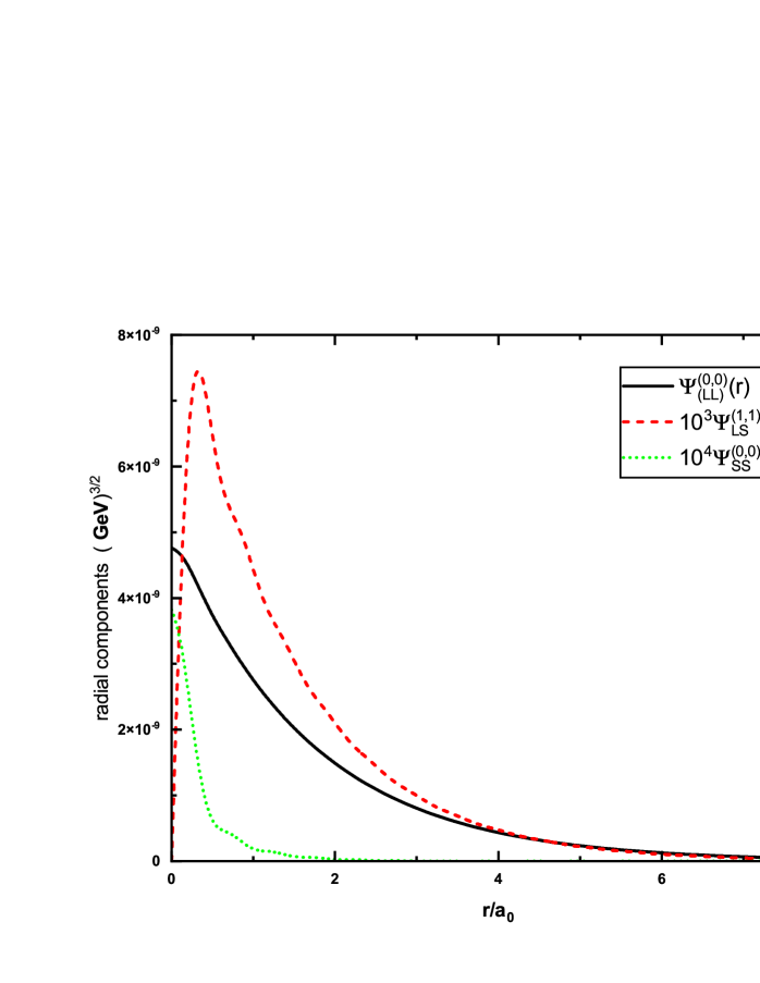
Figure 1: Radial wave-functions of the large-large (LL), large-small (LS) and small-small (SS) components of the para-Ps ground state.

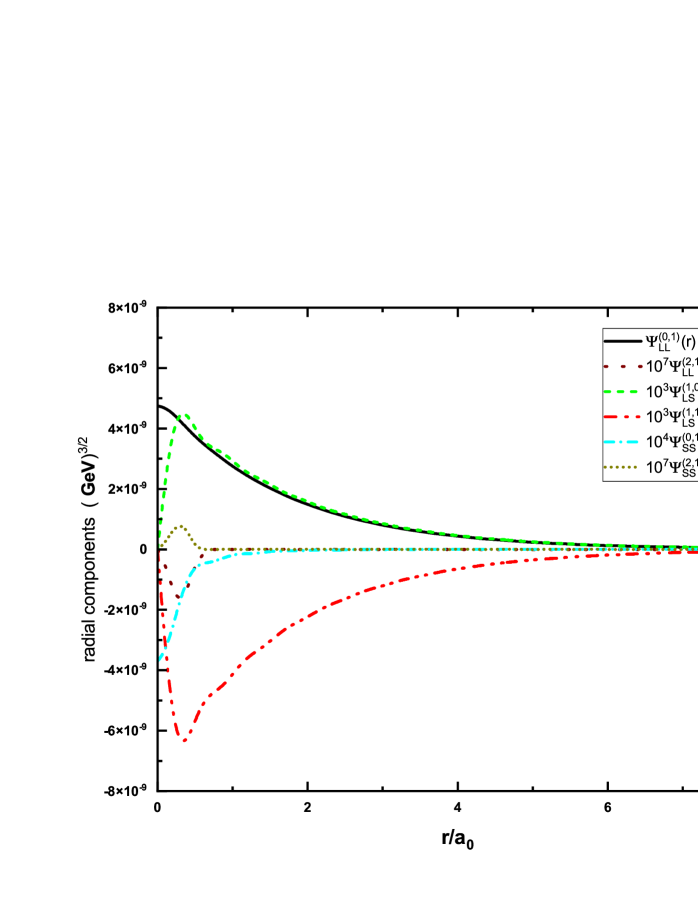
Figure 2: Radial wave-functions of the large-large (LL), large-small (LS) and small-small (SS) components of the ortho-Ps ground state.

In Fig.1 and Fig.2 the radial wave-functions of the large-large (LL), large-small (LS) and small-small (SS) components of the para-Ps and ortho-Ps ground states are presented, respectively. In the upper index of the radial function notations the corresponding spin-orbital channels are indicated. As can be noted, the behaviors of the radial wave functions of all the components of the para-Ps are close to main parts of the corresponding components of the ortho-Ps. In particular, the corresponding LL-components and the absolute values of the SS-components are almost identical, but the SS-components differ by the signatures. The LS-components of the ortho-Ps corresponding to different spin-orbital channels $\Psi_{LS}^{(1,0)}(r)$ and $\Psi_{LS}^{(1,1)}(r)$ are of the same form, but have opposite signs and differ by about 40% in the absolute values.

In Table 1 a convergence of the numerical results of calculations for the energy $E/2m_{e}$, binding energy $E_{b}$, weights of the components for breaking the $P$, $C$ and $CP$ symmetries in the para- and ortho-positronium ground-states are presented in respect to the maximal oscillator quantum number of basis sates $n_{max}$. The optimal value of the oscillator length $a_{0}=3.3\times 10^{5}$ GeV^-1. As can be seen from the table, all the parameters are well converged with increasing $n_{max}$. As noted above, the further increase of $n_{max}$ results in the collapse of the variational basis.

Table 1: Convergence of the numerical results for $E/2m_{e}$, $E_{b}$, weights of the components violating $P$, $C$ and $CP$ symmetries in the para- and ortho-positronium ground-states in respect to $n_{max}$.

State	$n_{max}$	$E/2m_{e}$	$E_{b}$ (eV)	$W_{P}$	$W_{C}$	$W_{CP}$
${}^{1}S_{0}$	10	0.9999935056580695	6.637203529	7.467E-6	0	7.467E-6
($p$-Ps)	20	0.9999933597022965	6.786370016	6.760E-6	0	6.760E-6
	30	0.9999933453955095	6.800991522	6.667E-6	0	6.667E-6
	35	0.9999933438924752	6.802527620	6.659E-6	0	6.659E-6
	37	0.9999933433568433	6.803075034	6.656E-6	0	6.656E-6
${}^{3}S_{1}$	10	0.9999935056580694	6.637203529	7.467E-6	4.978E-6	2.4892E-6
($o$-Ps)	20	0.9999933597022961	6.786370017	6.756E-6	4.504E-6	2.252E-6
	30	0.9999933453955091	6.800991522	6.666E-6	4.444E-6	2.222E-6
	35	0.9999933438924745	6.802527620	6.660E-6	4.440E-6	2.220E-6
	37	0.9999933433568923	6.803074984	6.656E-6	4.438E-6	2.218E-6

Table 2: Energies of the lowest states of the para- and ortho-Ps in comparison with the results of the finite-element method scott1992 .

$(\ell,S,J)$	$E/2m_{e}$	$E/2m_{e}$ scott1992
(0,0,0)	0.999 993 343 356 843	0.999 993 340 148 538 880
(0,1,1)	0.999 993 343 356 892	0.999 993 340 148 552 498
(1,1,0)	0.999 998 342 584 549	0.999 998 335 009 885 854
(1,0,1)	0.999 998 342 513 543	0.999 998 335 017 278 391

In Table 2 the energies of the lowest states of the para- and ortho-Ps are compared with the results of the finite-element method of high accuracy scott1992 . Of course, our variational method on the harmonic-oscillator basis is not very accurate as the finite-element method due-to the collapse of the variational basis at some value of $n_{max}$. The binding energies of the $p$-Ps and $o$-Ps ground states in our calculations are estimated to be 6.803075 eV, which should be compared with the values of 6.806403 eV for the para-Ps and 6.806354 eV for the ortho-Ps of Ref.scott1992 . This means that the precision of the energy calculations is of order $0.003$ eV, which is good enough for the application of corresponding wave functions to the estimation of the weights of the symmetry-violating terms in positronium as the norm-square of the corresponding components.

From Table 1 one can see that in the para-positronium the $P$ and $CP$ symmetry breaking terms have identical weights. The final result for the weights of the $P$ and $CP$ symmetry-violating components are estimated to be 6.656E-6. For the ortho-Ps, the weight of the $P$ symmetry-breaking components is identical to the case of para-Ps. On the other hand, the weight of the $P$ symmetry-breaking components is equal to the sum of the weights of the $C$- and $CP$- violating terms. At the same time, the weight of the $C$ symmetry-violating terms is twice the weight of the $CP$ symmetry-breaking components. And the final results for the weights of the $P$, $C$ and $CP$ symmetry violating components in the ortho-Ps are 6.656E-6, 4.438E-6, and 2.218E-6, respectively. Thus, the precision of order $10^{-4}$ of the results of experimental research work NatCom2024 and of order $10^{-3}$ of the data of Ref.yam2010 are still not enough for the observation of the $CP$ violation events in the ortho-positronium.

IV Summary

A new theoretical method was suggested to solve the two-body Dirac equation for positronium bound states. Only Coulomb potential was included into the Dirac Hamiltonian. It is shown that the two-body Hermitian Dirac Hamiltonian contains terms, responsible for violating the $P$, $C$ and $CP$ symmetries. Numerical results for the energy spectrum of the para- and ortho-positronium lowest states performed within the variational method using the harmonic oscillator basis functions are in good agreement with a high-precision finite-element method. The weights of the $P$ and $CP$ symmetry-violating components in the para-positronium ground state are identical to the weight of the $P$ symmetry-violating component of the ortho-Ps and estimated to be 6.6E-6. The weights of the $C$ and $CP$ symmetry-violating components of the ortho-Ps are equal to the 2/3 and 1/3 parts of this value, respectively. These numbers are less by two-order of magnitude than the precision limit of current experimental facilities.

References

• (1) S.D. Bass, S. Mariazzi, P. Moskal, E. Stepien, Rev. Mod. Phys. 95, 021002 (2023).
• (2) G.S. Adkins, D.B. Cassidy, J. Perez-Rios, Phys. Rep. 975, 1-61 (2022).
• (3) A.D. Sakharov, Pisma Zh. Eksp. Teor. Fiz. 5, 32 (1967), JETP Lett. 5, 24 (1967), Sov. Phys. Usp. 34, 392 (1991), Usp. Fiz. Nauk 161, 61 (1991).
• (4) J.H. Christenson, J.W. Cronin, V.L. Fitch, and R. Turlay, Phys. Rev. Lett. 13, 138 (1964)
• (5) M. Kobayashi and T. Maskawa, Prog. Theor. Phys. 49, 652 (1973).
• (6) T. Yamazaki, T. Namba, S. Asai, T. Kobayashi, Phys. Rev. Lett. 104, 083401 (2010).
• (7) A. Rubbia, Int. J. Mod. Phys. 19, 3961 (2004)
• (8) C Bartram and R Henning, J. Phys.: Conf. Ser. 1342, 012106 (2020).
• (9) T.-E. Haugen, E. A. George, O. Naviliat-Cuncic, and P. A. Voytas, EPJ Web of Conferences 282, 01003(2023).
• (10) P.A. Vetter, S. J. Freedman, Phys. Rev. A 66, 052505 (2002).
• (11) P. Moskal, E. Czerwinski, J. Raj et al. Nat. Commun. 15, 78 (2024).
• (12) W.E. Caswell, G.P. Lepage, Phys. Lett. B 167, 437 (1986).
• (13) A. Czarnecki, K. Melnikov, A. Yelkhovsky, Phys. Rev. Lett. 82, 311 (1999).
• (14) K. Pachucki, S.G. Karshenboim, Phys. Rev. Lett. 80, 2101 (1998).
• (15) A. Czarnecki, K. Melnikov, A. Yelkhovsky, Phys. Rev. A 59, 4316 (1999).
• (16) P. Labelle, Phys. Rev. D 58, 093013 (1998).
• (17) T.C. Scott, J. Shertzer, R. A. Moore, Phys. Rev. A 45, 4393 (1992)
• (18) D. Ferenc and E. Matyus, Phys. Rev. A bf 107, 052803 (2023).
• (19) C.W. Patterson, Phys. Rev. A 100, 062128 (2019).
• (20) C.W. Patterson, Phys. Rev. A 107, 042816 (2023).
• (21) H.W. Crater, C.Y. Wong, P. Van Alstine, Phys. Rev. D 74, 054028 (2006).
• (22) H.W. Crater, Jin-Hee Yoon, Cheuk-Yin Wong, Phys. Rev. D 79, 034011 (2009).
• (23) Th. Gutsche and D. Robson, Phys. Lett. B 229, 333 (1989).
• (24) Th. Gutsche. A chiral potential model for the light-quark baryons. Ph.D thesis, Florida State University, 249 p. (1987).
• (25) E.M. Tursunov, J. Phys. G 36, 095006 (2009).
• (26) E.M. Tursunov, and S. Krewald, Phys. Rev. D 90, 074015 (2014).