UDE-based Dynamic Motion/Force Control of Mobile Manipulators

Abstract

Mobile manipulators are known for their superior mobility over manipulators on fixed bases, offering promising applications in smart industry and housekeeping scenarios. However, the dynamic coupling nature between the mobile base and the manipulator presents challenges for the physical interactive tasks of the mobile manipulator. Current methods suffer from complex modeling processes and poor transferability. To address this, this article presents a novel dynamic model of the manipulator on the mobile base that requires only the manipulator dynamics and the kinematic information of the mobile base. In addition, embedding the dynamic model, an uncertainty and disturbance estimator-based (UDE-based) dynamic motion/force control scheme is proposed for the mobile manipulator, which compensates for the dynamic coupling and other unmodeled uncertainties. Passivity and stability analyses justify the proposed control law. Simulation and experimental results on our mobile manipulator platform demonstrate the feasibility and effectiveness of our proposed methodology.

I Introduction

The integration of a manipulator on the mobile base, commonly known as a mobile manipulator, has greatly expanded the manipulator’s workspace and gained popularity recently due to its enhanced mobility and interaction capabilities. It has various applications such as housekeeping [1, 2, 3], industrial inspection [4, 5], underwater exploration [6, 7, 8, 9], mine exploring [10], search and rescue [11], and so on.

In most scenarios, the common approach to control the mobile manipulator involves moving the mobile base to the desired location and then executing the interactive task with the manipulator. Although this method of control is straightforward, it has limitations in some application contexts. For example, in manufacturing and maintenance tasks, there is a need for contact-based inspection of large parts for defect detection and quality inspections, where the mobile manipulator needs to cover a large workspace and track the surface of the parts. Such tasks require mobility in the manipulator’s operations, and the aforementioned method cannot fulfill these types of tasks. Moreover, in industrial settings, enhancing the efficiency of mobile manipulators can significantly reduce the overall demand for these robots, thereby increasing factory productivity [12].

To simultaneously manage mobility and interaction tasks, the main challenge lies in the nonlinear dynamic coupling between the mobile base and the manipulator system. When motion changes dynamically in the mobile base, the manipulator generates undesired movement that leads to performance degradation [10] and potential collisions [13].

Some studies model the dynamic coupling effects between the mobile base and the manipulator in the whole-body dynamics and employ robust controllers to restrain other unmodeled uncertainties [10, 14, 15]. For instance, in [10], an $H_{\infty}$ controller augmented with a feedforward term is applied to restrain the undesired motion of the compliant forklift and the terrain-induced disturbance. This helps to reduce material spillage when the forklift is operating on uneven ground. In [14], a whole-body dynamic model is formed to address the holonomic and non-holonomic constraints of the mobile manipulator. At the same time, the adaptive neural network (NN) control is adopted to compensate for the unmodeled dynamics and disturbance. In [15], the coupled dynamic model of the mobile manipulator is established with physical human-robot interaction (pHRI) considered, and the force/torque of the mobile manipulator is monitored to prevent safety issues.

However, modeling the whole-body dynamics of the mobile manipulator system could be challenging [16]. According to [14], the base and the manipulator dynamic behaviors are different. The mobile base is typically propelled by a combination of multiple actuators, which contrasts with the most common form of manipulators driven by a series of actuators connected in a chain. Meanwhile, ground vehicles operate under unique constraints such as nonholonomic constraints that limit their movement. These factors contribute to the complexity and difficulty of whole-body modeling. The challenges lead to the high cost of developing effective and universally applicable solutions, which severely limits the transferability of whole-body modeling across different mobile manipulator platforms.

While work in mobile manipulators primarily focuses on whole-body dynamics, there are distinct approaches observed in aerial manipulators [17, 18]. In [17], variable inertia parameters are employed to describe the dynamic coupling effects caused by the mass distribution offset of the manipulator. The $H_{\infty}$ controller compensates the dynamic coupling to stabilize the unmanned aerial vehicle (UAV) during the dynamic motion of the manipulator. A parallel aerial manipulator is proposed in [18], where manipulator dynamics is compensated in the aerial vehicle’s pose controller. Nevertheless, these works are mainly constrained to motion control of the aerial manipulator without considering the force interaction with environments and continue to face challenges with model transferability.

Existing methods suffer from complex modeling processes and poor transferability. To address this, drawing inspiration from the aerial manipulator approach, we consider the dynamic coupling effects in manipulator dynamics and ignore effects on the mobile base. We assume that for mobile manipulators, the stability of the mobile base guarantees that the manipulator’s motions do not affect the base’s mobility. Moreover, our method requires only the manipulator dynamics and the kinematic information of the mobile base, which simplifies the complexity of system modeling and improves its transferability. Our method represents a novel direction in the field. In addition, we extend the methodologies in [19] from manipulators to mobile manipulators and introduce an uncertainty and disturbance estimator-based (UDE-based) dynamic motion/force control scheme, incorporating feedback and feedforward control mechanisms. The contributions of this article are concluded as follows:

• A novel dynamic model of the manipulator on the mobile base is proposed, where dynamic coupling effects are modeled by incorporating the kinematic information of the mobile base into the manipulator dynamics.

• Embedding our model, a UDE-based dynamic motion/force controller of the manipulator is proposed to improve the dynamic performance of the robot-environment interaction (REI) system. The feedforward control law is applied to predict dynamic coupling between the mobile base and the manipulator, and UDE compensates for other unmodeled uncertainties.

• Comparative simulations and experiments verify the dynamic model of manipulators, the motion/force tracking performance of the proposed control law, and its ability to withstand dynamic coupling effects.

The rest of the article is organized as follows: Sec II formulates the dynamic model of the manipulator on the mobile base. Sec III introduces the UDE-based dynamic motion/force control law design for the manipulator. Sec IV demonstrates the effectiveness of the proposed control law through simulations and experiments. Finally, Sec V concludes this article.

II Dynamic modeling of manipulator on the mobile base

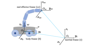
Figure 1: The mobile manipulator platform and the coordinate systems: the inertial frame $\{i\}$, the body frame $\{b\}$, and the end effector frame $\{ee\}$. The forward and yaw speed of the mobile base expressed in $\{b\}$ is given by $v$ and $w$.

In this section, we consider the dynamic coupling effects in the manipulator dynamics. Firstly, consider a $n$-degree of freedom (DOF) manipulator attached to a moving base, as shown in Fig. 1. The body frame $\{b\}$ centers at the center of gravity (CG) of the mobile base, denoted by $O_{b}$, and the end effector frame $\{ee\}$ centers at the CG of the end effector of the manipulator, namely $O_{ee}$. First, we develop the dynamic equation of the manipulator based on the Euler-Lagrange method:

$$M_{q}\ddot{q}+C_{q}\dot{q}+G_{q}=\tau+\hat{J}^{T}f_{e},$$ (1)

where $q\in\mathbb{R}^{n}$ denotes the joint vector of the manipulator. $M_{q}$, $C_{q}\dot{q}$, $G_{q}$ represents the inertial, the Coriolis and centrifugal forces, and the gravity term. $\tau\in\mathbb{R}^{n}$ represents the input torque vector exerted on the joint, while $f_{e}=[f_{x},f_{y},f_{z},f_{m},f_{n},f_{k}]^{T}\in\mathbb{R}^{6}$ is expressed in $\{i\}$ and accounts for wrenches due to the contact with the environment. $\hat{J}=\begin{bmatrix}{R^{i}_{b}}&\mathbf{0}\\ \mathbf{0}&{R^{i}_{b}}\end{bmatrix}J$ is the augmented Jacobian matrix, where $J$ represents the analytic Jacobian matrix of the manipulator and $R^{i}_{b}$ denotes the rotation matrices of frame $\{i\}$ with respect to $\{b\}$.

Furthermore, the Cartesian coordinates of the mobile manipulator expressed in the inertial frame $\{i\}$ are given by $X=\begin{bmatrix}\eta\\ x\end{bmatrix}\in\mathbb{R}^{12}$, where $\eta=\begin{bmatrix}p_{\eta}\\ \Theta_{\eta}\end{bmatrix}=[\eta_{1},\eta_{2},\eta_{3},\eta_{4},\eta_{5},\eta_{6}]^{T}\in\mathbb{R}^{6}$ are the Cartesian coordinates of the mobile base and $x=\begin{bmatrix}p_{x}\\ \Theta_{x}\end{bmatrix}=[x_{1},x_{2},x_{3},x_{4},x_{5},x_{6}]^{T}\in\mathbb{R}^{6}$ are the Cartesian coordinates of the end effector of the manipulator.

Let $\phi(t;0,x_{d}(0),\dot{x}_{d}(0),f_{e,d}(0))$ represent the desired trajectory of the end effector of the manipulator during the time interval $[0,t]$ with an initial state $x_{d}(0),\dot{x}_{d}(0),f_{e,d}(0)$. The task of the mobile manipulator is to track the motion/force trajectory $\phi(t;0,x_{d}(0),\dot{x}_{d}(0),f_{e,d}(0))$ in Cartesian space for the end effector while maintaining the compliance of the end effector and compensating dynamic coupling effects and other unmodeled uncertainties during operation.

Based on Fig. 1, the kinematic relation between $\eta$ and $x$ is given by:

$$p_{x}=p_{\eta}+ P^{i}_{ee/b}=p_{\eta}+R^{i}_{b}P^{b}_{ee/b},$$ (2)

$$R^{i}_{ee} =R^{i}_{b}R^{b}_{ee},$$ (3)

where $R^{i}_{b}$, $R^{b}_{ee}$, $R^{i}_{ee}$ are the rotation matrices of frame $\{i\}$ with respect to $\{b\}$, $\{b\}$ with respect to $\{ee\}$, $\{i\}$ with respect to $\{ee\}$. $P^{b}_{ee/b}$ denotes the position of the end effector with respect to the body frame $\{b\}$ expressed in $\{b\}$ and $P^{i}_{ee/b}$ denotes the position of the end effector with respect to the body frame $\{b\}$ expressed in $\{i\}$.

Take the derivative of (1) yields:

$$\dot{p}_{x}=\dot{p}_{\eta}+R^{i}_{b}\dot{P}^{b}_{ee/b}+\omega^{i}_{ee/b}\times P^{i}_{ee/b},$$ (4)

where $\omega^{i}_{b/b}$ denotes the angular velocity of the end effector with respect to the body frame $\{b\}$ expressed in $\{b\}$, and $``\times"$ denotes the cross-product operator.

Take the derivative of (2) yields:

$$\omega^{i}_{ee/i}=\omega^{i}_{b/i}+R^{i}_{b}\omega^{b}_{ee/b}.$$ (5)

Combining (4) and (5), the kinematic relation between $\dot{\eta}$ and $\dot{x}$ is expressed as follows:

$$\dot{x}=\dot{\eta}+\begin{bmatrix}{R^{i}_{b}}&\mathbf{0}\\ \mathbf{0}&{R^{i}_{b}}\end{bmatrix}\begin{bmatrix}\dot{p}^{b}_{ee/b}\\ \omega^{b}_{ee/b}\end{bmatrix}+\begin{bmatrix}\omega^{i}_{ee/b}\times P^{i}_{ee/b}\\ 0\end{bmatrix}.$$ (6)

Consider the transformation of the manipulator between joint space and Cartesian space:

$$\begin{bmatrix}\dot{p}^{b}_{ee/b}\\ \omega^{b}_{ee/b}\end{bmatrix}=J(q)\dot{q}.$$ (7)

Substituting (7) into the kinematic equation (6), the overall kinematic equation can be rewritten as:

$$\dot{x}=\dot{\eta}+\hat{J}\dot{q}+d,$$ (8)

where $d=\begin{bmatrix}\omega^{i}_{ee/b}\times P^{i}_{ee/b}\\ 0\end{bmatrix}$.

The derivative of (8) is given by:

$$\ddot{x}=\ddot{\eta}+\dot{\hat{J}}\dot{q}+\hat{J}\ddot{q}+\dot{d}.$$ (9)

To directly control the motion and force of the end effector, according to the kinematic relationship (8) and the derivative (9), multiplying $(\hat{J}^{\dagger})^{T}$ on both sides of (1) yields the task space dynamic model of the manipulator on the moving base:

$$M_{0}(\ddot{x}-\ddot{\eta}-\dot{d})+C_{0}(\dot{x}-\dot{\eta}-d)+G_{0}=f+f_{e},$$ (10)

where $M_{0}=(\hat{J}^{\dagger})^{T}M\hat{J}^{\dagger}$ , $C_{0}=(\hat{J}^{\dagger})^{T}C\hat{J}^{\dagger}-(\hat{J}^{\dagger})^{T}M\hat{J}^{\dagger}\dot{\hat{J}}\hat{J}^{\dagger}$, $G_{0}=(\hat{J}^{\dagger})^{T}G$, and $f=(\hat{J}^{\dagger})^{T}\tau$. The equations of motion (8) and (10) provide a direct means to design a Cartesian controller for the manipulator on the moving base.

III UDE-based Dynamic Motion/Force Controller Design

This section proposes a novel feedback-feedforward control strategy to compensate for dynamic coupling and various unmodeled uncertainties during the movement of the mobile base. The overall control diagram of the proposed UDE-based dynamic motion/force controller is illustrated in Fig. 2. Specifically, the feedforward term $f_{FF}$ predicts the dynamic coupling effects, thereby improving the dynamic response of the REI system. On the other hand, the feedback term $f_{UDE}$ maintains the system’s stability and enhances system performance by estimating unmodeled dynamics.

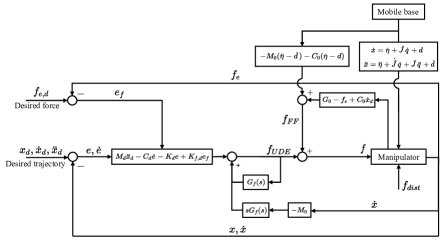
Figure 2: Control diagram of the proposed UDE-based dynamic motion/force control law.

III-A Feedforward controller design

A feedforward controller, denoted as $f_{FF}$, is proposed to predict and compensate for dynamic coupling effects and other modeled disturbances, which can improve the dynamic response of the mobile manipulator system. Based on the dynamic model of the manipulator on the mobile base (10), the base-manipulator coupling effects are expressed as $-M_{0}(\ddot{\eta}+\dot{d})-C_{0}(\dot{\eta}+d)$. The feedback linearization term, $G_{0}-f_{e}+C_{0}\dot{x}_{d}$, compensates for the gravity and the external wrench exerted on the manipulator and ensures the tracking of the desired impedance behavior.

Consequently, the overall feedforward term $f_{FF}$ is given by:

$$f_{FF}=-M_{0}(\ddot{\eta}+\dot{d})-C_{0}(\dot{\eta}+d)+G_{0}-f_{e}+C_{0}\dot{x}_{d},$$ (11)

which combines the compensation terms for the dynamic coupling effects, gravity, and external wrench.

III-B UDE design

In practice, obtaining accurate dynamic model parameters can be challenging. To further improve the disturbance rejection ability of the mobile manipulator system, UDE is proposed to compensate for dynamic coupling between the mobile base and the manipulator, as well as other unmodeled uncertainties.

The mobile manipulator system is designed to exhibit the impedance behavior at the end effector [20]. Specifically, the desired impedance behavior is expressed in the form of:

$$M_{d}(\ddot{x}-\ddot{x}_{d})+C_{d}\dot{e}+K_{d}e=K_{f,d}e_{f},$$ (12)

where $M_{d}$, $C_{d}$, $K_{d}$, $K_{f,d}$ represents the inertial, damping, stiffness, and force matrix. Motion and force error terms is defined as $e={x}-{x}_{d}$, $e_{f}=f_{e}-f_{e,d}$. Without loss of generality, we select $M_{d}=M_{0}$, which yields:

$$M_{0}(\ddot{x}-\ddot{x}_{d})+C_{d}\dot{e}+K_{d}e=K_{f,d}e_{f}.$$ (13)

Adding $f_{UDE}$ on both sides of the desired impedance model (13) yields:

$$\begin{split}f_{UDE}=M_{0}\ddot{x}_{d}-(C_{d}\dot{e}+K_{d}e-K_{f}e_{f})-(M_{0}\ddot{x}-f_{UDE}).\end{split}$$ (14)

Let $\mu_{d}=M_{0}\ddot{x}-f_{UDE}$, and according to [19], $\mu_{d}$ denotes all unmodeled uncertainties in the system. Then:

$$f_{UDE}=(M_{0}\ddot{x}_{d}-C_{d}\dot{e}-K_{d}e+K_{f,d}e_{f})-\mu_{d}.$$ (15)

Assuming that the system dynamics and the unmodeled disturbance are limited below a cutoff frequency $\omega_{c}$, then uncertainties $\mu_{d}$ can be estimated with an ideal low-pass filter $G_{f}(s)$:

$$\hat{\mu}_{d}=\mathbf{L}^{-1}\{G_{f}(s)\}\ast(M_{0}\ddot{x}-f_{UDE}).$$ (16)

where $``\ast"$ represents the convolution symbol and $\mathbf{L}^{-1}$ represents the inverse Laplace transform symbol. $G_{f}(s)$ has an unit gain and zero phase shift when $\omega\leq\omega_{c}$ and zero gain when $\omega>\omega_{c}$. Zero estimation error is thus guaranteed in both scenes when $\omega\leq\omega_{c}$ and $\omega>\omega_{c}$. In other words:

$$\begin{split}\mu_{d}-\hat{\mu}_{d}=\mathbf{L}^{-1}\{1-G_{f}(s)\}\ast(M_{0}\ddot{x}-f_{UDE})=0.\end{split}$$ (17)

This indicates that UDE can effectively estimate unmodeled uncertainties in the system, thus improving the disturbance rejection ability of the mobile manipulator system.

Substituting (16) and (17) in (15) yields:

$$\begin{split}f_{UDE}=&(M_{d}\ddot{x}_{d}-C_{d}\dot{e}-K_{d}e+K_{f,d}e_{f})\\ &-\mathbf{L}^{-1}\{G_{f}(s)\}\ast(M_{0}\ddot{x}-f_{UDE}).\end{split}$$ (18)

And the final input $f_{UDE}$ is given by:

$$\begin{split}f_{UDE}=&\mathbf{L}^{-1}\{\frac{1}{1-G_{f}(s)}\}\ast(M_{0}\ddot{x}_{d}-C_{d}\dot{e}-K_{d}e+K_{f,d}e_{f})\\ &-\mathbf{L}^{-1}\{\frac{G_{f}(s)}{1-G_{f}(s)}\}\ast M_{0}\ddot{x}\\ =&\mathbf{L}^{-1}\{\frac{1}{1-G_{f}(s)}\}\ast(M_{0}\ddot{x}_{d}-C_{d}\dot{e}-K_{d}e+K_{f,d}e_{f})\\ &-\mathbf{L}^{-1}\{\frac{sG_{f}(s)}{1-G_{f}(s)}\}\ast M_{0}\dot{x}.\end{split}$$ (19)

Note that the UDE-based control law (19) relies solely on velocity rather than acceleration information, making it easier to implement in practice. In the proposed control law, UDE is utilized as a compensator within the controller, allowing it to estimate the dynamic coupling and other disturbances by filtering system inputs and states.

III-C Stability analysis

Theorem III.1.

Under the control law (20), the manipulator system on the mobile base (10) is guaranteed to be globally asymptotic stable in the full motion control mode and stable and able to achieve the desired hybrid impedance model (13) in motion/force control mode.

$$f=f_{UDE}+f_{FF}.$$ (20)

Proof.

Consider a Lyapunov candidate:

$$V=\frac{1}{2}\dot{e}^{T}M_{0}\dot{e}+\frac{1}{2}{e}^{T}K_{d}e.$$ (21)

The first derivative of the Lyapunov candidate $V$ is given by:

$$\begin{split}\dot{V}&=\dot{e}^{T}\left(M_{0}\ddot{e}+\frac{1}{2}\dot{M}_{0}\dot{e}\right)+{e}^{T}K_{d}\dot{e}.\end{split}$$ (22)

Substituting the dynamic model of the manipulator on the moving base (10) to (22) yields:

$$\begin{split}\dot{V}=&\dot{e}^{T}(M_{0}(\ddot{\eta}+\dot{d})+C_{0}(\dot{\eta}+d)-C_{0}\dot{x}-G_{0}+f_{e}+f\\ &-M_{0}\ddot{x}_{d}+\frac{1}{2}\dot{M}_{0}\dot{e})+{e}^{T}K_{d}\dot{e}.\end{split}$$ (23)

Substituting control law $f$ (20) into (23) produces:

$$\begin{split}\dot{V}=&\dot{e}^{T}(-C_{0}\dot{e}+\frac{1}{2}\dot{M}_{0}\dot{e}-M_{0}\ddot{x}_{d}+K_{d}e\\ &+\mathbf{L}^{-1}\{\frac{1}{1-G_{f}(s)}\}\ast(M_{0}\ddot{x}_{d}-C_{d}\dot{e}-K_{d}e+K_{f,d}e_{f})\\ &-\mathbf{L}^{-1}\{\frac{G_{f}(s)}{1-G_{f}(s)}\}\ast M_{0}\ddot{x}).\end{split}$$ (24)

Using the desired impedance behavior (13) leads to:

$$\begin{split}\dot{V}&=\dot{e}^{T}(-C_{d}\dot{e}+K_{f,d}e_{f}).\end{split}$$ (25)

Rewrite (25), we obtain:

$$\begin{split}\dot{V}=-\dot{e}^{T}C_{d}\dot{e}+\dot{e}^{T}K_{f,d}e_{f}\leq\dot{e}^{T}K_{f,d}e_{f}.\end{split}$$ (26)

It can be concluded from (26) that when the REI system is in full motion control mode, i.e., $K_{f,d}=0$, we have $\dot{V}=-\dot{e}^{T}C_{d}\dot{e}$, which is negative semi-definite. According to the Lyapunov stability theorem, the system is globally asymptotic stable. When the system is in motion/force control mode, the close-loop system (1) (13) (20) is a passive system, which ensures a stable behavior. This completes the proof. ∎

IV Simulation and Experiment

To evaluate the effectiveness and dynamic performance of the UDE-based dynamic motion/force control scheme, three controllers are selected for simulation and experiment studies, namely C1, C2, and C3.

• C1: the proposed control law, UDE-based dynamic motion/force control scheme (20) (UDE-based controller incorporated with the dynamic model (10) and feedforward base information);

• C2: IC law incorporated with our dynamic model and feedforward base information;

• C3: IC.

IV-A Simulation results

Comparisons of C1, C2, and C3 are operated in the simulation to verify the proposed model and the proposed control law. The controller runs at a speed of $180$ Hz, and the simulation studies were operated on an open-source Gazebo simulator.

IV-A1 Prediction of the dynamic coupling effects

(a)

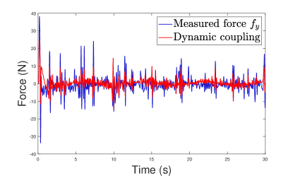
(b)

Figure 3: Comparison of the dynamic coupling effects and the proposed model for $30s$ at $180Hz$.

In the first simulation, the proposed dynamic model is validated. The mobile base is assigned to move a sine trajectory, and the force sensor is equipped between the manipulator and the mobile base to measure dynamic coupling effects.

The comparison between ground truth and the predicted wrenches, i.e., the dynamic coupling effects are shown in Fig. 3. We quantified the discrepancies using weighted mean absolute percentage deviations (wMAPDs)in the $x$ and $y$ directions, which amounted to $81.51\%$ and $80.12\%$, respectively. The findings substantiate the efficacy of our proposed model, with the residual discrepancies primarily due to noisy sensors and unmodeled uncertainties.

IV-A2 Dynamic motion/force tracking of the manipulator under dynamic coupling effects

In this simulation, comparisons are conducted among three controllers to verify the proposed UDE-based dynamic motion/force control scheme’s effectiveness and ability to withstand dynamic coupling effects and other unmodeled uncertainties.

The mobile base moves on rough terrain at a surging speed of $0.2$ m/s, which causes random changes in its movement and leads to undesired motions of the manipulator. This can be observed in the disturbances recorded by lateral $\eta_{2}$ motion of the mobile base, as illustrated in Fig. 4 (a).

The manipulator is tasked to move toward the wall along the predefined motion trajectory $\phi(t;0,x_{d}(0),\dot{x}_{d}(0),f_{e,d}(0))$. Once in contact with the wall, it follows a motion trajectory and applies forces of $5$ N and $10$ N on the wall, respectively. For controller C1, $G_{f}$ is selected as a first-order low-pass filter $G_{f}=\frac{\omega_{c}}{s+\omega_{c}}$ and $\omega_{c}$ is selected as 6 in the setup. For controllers C1, C2, and C3, the impedance parameters are initialized as $K_{d}=[200,200,200,20,20,20]$, $D_{d}=[2,2,2,1,1,1]$, $K_{f,d}=[0,5,0,0,0,0]$.

The mobile manipulator initially operates in full motion control mode with the desired force $f_{e,d}=0N$ and the desired motion trajectory $x_{2,d}=0.4m$. It then transitions to impedance control mode at $20$s by changing the desired motion/force trajectory. The manipulator is commanded to exert $f_{e,d}=5N$ force on the wall and follow a motion trajectory $x_{2,d}=0.6m$ in the y-axis. The desired force increases to 10 N at $30$s and returns to 5N at $40$s. After the wiping task finishes, the manipulator gradually returns to full motion control at $50$s by reverting the desired force to $f_{e,d}=0N$ and the desired motion to $x_{2,d}=0.4m$.

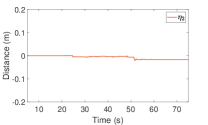
(a)

(b)

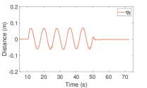
(c)

(d)

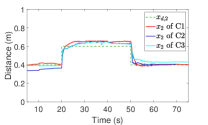
(e)

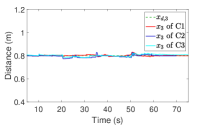
(f)

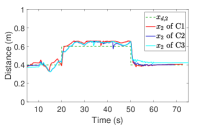
(g)

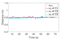
(h)

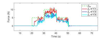
(i)

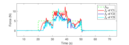
(j)

Figure 4: Comparative motion/force tracking results of simulation 1 and simulation 2 among C1, C2, and C3. (a), (b), (e), (f), and (i) belong to simulation 1, while (c), (d), (g), (h), and (j) belong to simulation 2. (a) and (c) is the lateral position $\eta_{2}$ of the mobile base in simulation 1 and simulation 2. (b), (e), (f) and (d), (g), (h) are the comparative results of position tracking, while (i) and (j) are the comparative results of force tracking in Simulation 1 and Simulation 2.

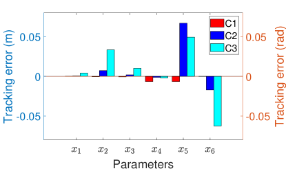
(a)

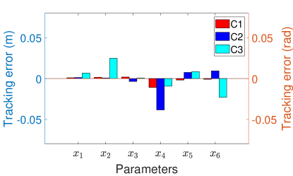
(b)

Figure 5: Motion tracking error of C1, C2, and C3 in two simulations in full motion control. (a) Motion tracking error in simulation 1. (b) Motion tracking error in simulation 2. C1 achieves the lowest motion tracking error in both simulations, compared to C2 and C3, except for the $x_{4}$ in the second simulation.

TABLE I: Force tracking performance of three controllers in two simulations. The contents in brackets indicate the percentage improvement compared to the metrics of C1 (the first row).

	Simulation 1			Simulation 2
Controller	RMSE	MAD	SSE	RMSE	MAD	SSE
C3	11.3141	1.0870	3.0172	11.5719	1.3400	2.9437
C2	9.5819 (15.31%)	0.8476 (22.02%)	2.8081 (6.93%)	10.4534 (9.67%)	0.9811 (26.78%)	2.8479 (3.25%)
C1	2.8968 (74.40%)	0.6035 (44.48%)	1.1531 (61.78%)	2.7134 (76.55%)	0.6293 (53.04%)	1.0522 (64.26%)

Results of the first simulation are shown in Fig. 4 (b), (e), (f), and (i) and 5 (a). As shown in Fig. 4 (b), (e), (f) and 5 (a), when the end effector returns to the full motion control ($t>55s$), motions of C1 converge to the setpoint while motions of C2 and C3 deviate from the setpoint due to the static friction of the joints. The performance of C2 is marginally better than that of C3, except for the pitch $x_{5}$, which demonstrates the effectiveness of the feedforward base information and the dynamic model (10). Moreover, C1 achieves the lowest motion tracking error compared to C2 and C3, maintaining negligible tracking errors, which validates the motion tracking ability of C1.

Quantitative evaluation of force tracking performance of three different controllers across two simulations is shown in Table I. Force tracking performance is measured by three metrics: root mean squared error (RMSE), mean absolute deviation (MAD), and steady-state error (SSE). The RMSE indicates the root squared difference error between the state and the setpoint, which is sensitive to outliers. A low RMSE suggests higher accuracy. The MAD measures the average difference between the state and the mean of the state. A small MAD suggests a tighter clustering of the state, signifying higher stability and consistency. Additionally, a low SSE signifies that the system more closely achieves its setpoint in the steady state.

Overall, C1 outperforms C2 and C3 in all three metrics. For Simulation 1, the RMSE of C1 and C2 improved by approximately 74.40% and 15.31% compared to C3, and the MAD of C1 and C2 improved by approximately 44.48% and 22.02% compared to C3. The results show that, under dynamic coupling effects (rough terrain and the moving base), C1 demonstrated the best performance in the simulation, with the lowest RMSE, MAD, and SSE, indicating it has a superior force tracking ability compared to C2 and C3 under base motions.

IV-A3 Motion/Force tracking under large base motions

In the third simulation, the mobile base moves forward at a constant speed of 0.2m/s, and the manipulator is required to track a given motion/force trajectory. In addition, to further examine the impact of significant motion changes on the mobile base, the mobile vehicle now follows a $sine$ trajectory in the $y$-axis. The motion of the mobile vehicle is illustrated in Fig. 4 (c).

Results of the second simulation are shown in Fig. 4 (d), (g), (h), and (j) and  5 (b). As shown in Fig. 4 (d), (g), and (h) and 5 (b), in the second simulation, C1 achieves the lowest motion tracking error compared to C2 and C3, except for the roll $x_{4}$. This demonstrates its motion tracking ability despite repeated steering of the mobile base. In addition, as shown in Fig. 4 (j), C1 achieves superior force tracking performance compared to C2 and C3. As shown in Table I, for Simulation 2, the RMSE of C1 and C2 improved by approximately 76.55% and 9.67% compared to C3, and the MAD of C1 and C2 improved by approximately 53.04% and 26.78% compared to C3.

From Simulation 1 to Simulation 2, the RMSE of C2 increased from 9.5819 to 10.4534, which is slightly better than the RMSE of C3 in Simulation 2 (11.5719). It shows limitations of the feedforward control in maintaining optimal performance when faced with significant external disturbances.

However, in contrast to the limitations in C2, the performance of C1 demonstrates a different trend. The minimal increase in MAD (increases by 4.28%) of C1 indicates superior performance, especially when compared to the significant increases in MAD observed in C2 (increases by 15.75%) and C3 (increases by 23.28%). Importantly, C1 maintained a small MAD and reduced in both RMSE and SSE, which further suggests that C1 is more robust and effective in managing large deviations, particularly under large base motions.

IV-B Experiment results

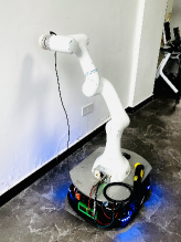
Figure 6: Experiment setup. The end effector is equipped with a 6-axis force sensor and a cleaning tool, and the mobile manipulator is tasked to follow a motion/force trajectory along the rigid wall.

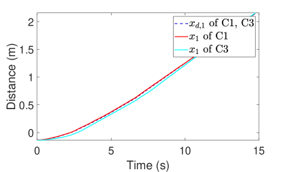
(a)

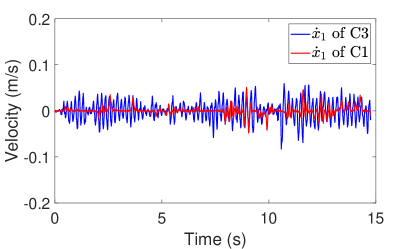
(b)

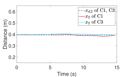
(c)

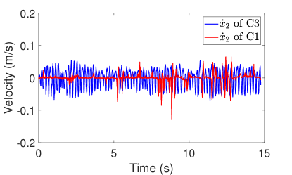
(d)

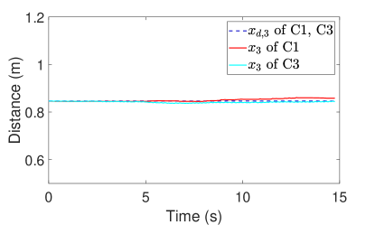
(e)

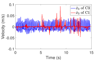
(f)

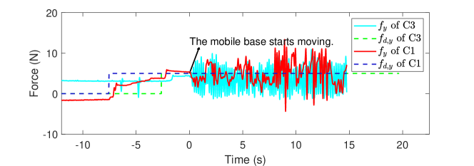
(g)

Figure 7: Comparative motion/force tracking results of the experiment. (a), (c), (e) are the comparative results of position tracking between C1 and C3, while (b), (d), (f) are the comparative results of the velocity between C1 and C3. (g) denotes the comparative results of force tracking between C1 and C3.

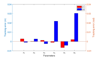
Figure 8: Motion tracking error of C1 and C3 in the experiment in full motion control.

TABLE II: Force tracking performance of two controllers in the experiment. The contents in brackets indicate the percentage improvement compared to the metrics of C1 (the first row).

	Experiment
Controller	RMSE	MAD	SSE
C3	8.3417	2.0913	1.4029
C1	5.3426 (35.95%)	1.9324 (7.60%)	-0.0696 (95.04%)

To further demonstrate the motion/force tracking performance of mobile manipulators’ proposed UDE-based dynamic motion/force, experiments are conducted using a mobile manipulator with an Atien TT15 mobile base and a Rokae SR3 manipulator. The experiment platform is shown in Fig. 6. The end effector is equipped with a 6-axis force sensor, and to replicate the practical working environment, a cleaning tool is mounted at its end. In the experiment, The mobile manipulator is tasked to swipe the rigid wall and apply a force of $5N$ against the wall while the mobile base moves along it. The maximum torque output in the experiment is limited to $[6,6,3,2,2,2]N\cdot m$ for safety considerations.

For controller C1, $\omega_{c}$ is selected as 3. The impedance parameters remain $K_{d}=[25,25,25,2.5,2.5,2.5]$, $D_{d}=[10,10,10,1,1,1]$, $K_{f,d}=[0,1,0,0,0,0]$. At $t=10s$, values of $e_{f,d}$ are gradually changed through a ramp function from $0N$ to $5N$. After changing the desired force, the mobile base starts to move along the wall at a forward speed of $0.16m/s$.

The motion/force tracking results of C1 and C3 are shown in Fig. 7, 8, and quantitative results are shown in Table II. Fig. 7 (a)-(f) and 8 shows that C1 exhibits commendable motion tracking capabilities compared to C3 by successfully keeping all tracking errors within 0.01 meters and radians.

For the force tracking performance, notably, C1 almost eliminates the SSE (-0.0696$N$) while the SSE of C3 is 1.4029$N$. During the movement of the mobile base, C3 exhibited oscillations, whereas C1 effectively mitigates this behavior. These observations imply that the proposed method is proficient in compensating for the dynamic coupling and other unmodeled uncertainties during the mobile base’s movement.

Moreover, the RMSE and MAD of C1 improve by approximately 35.95% and 7.60% compared to C3. The substantial improvement in RMSE suggests that C1 was particularly effective in reducing the magnitude of more significant errors. The slight improvement in MAD indicates that while C1 also reduced the average error, the improvement was not significant when considering minor deviations. This indicates that C1 is adept at minimizing errors within a smaller range.

IV-C Discussion

The simulation and experiment results reveal that the proposed control law C1 provides a more robust and effective control approach for mobile manipulators compared to C2 and C3.

However, it’s noteworthy that environmental stiffness and damping were set to mimic soft materials in the simulations. Under such conditions, the equilibrium point of interaction between the mobile manipulator and the environment shifts. This is evident in Fig. 4 (e) and Fig. 4 (g), where the position $x_{2}$ of the end effector exceeds $x_{2,d}$, and there’s a noticeable deviation of the actual force from the tracked value. Conversely, in the experiment, the mobile manipulator is tasked to swipe the rigid wall, and the environmental parameters are more substantial, ensuring that the force trajectory remains closely aligned with the set course. This indicates the limitation of this proposed method, and such deviation happens especially when interacting with soft environments.

V Conclusion

In this article, we present a novel dynamic model of the manipulator on the mobile base by incorporating the base kinematic information into the manipulator dynamics. Our method requires only the manipulator dynamics and the kinematic information of the mobile base, which simplifies the complexity of system modeling and improves its transferability. Moreover, embedding our dynamic model, a UDE-based dynamic motion/force control scheme is proposed to improve the dynamic performance of the mobile manipulator system, which compensates for the dynamic coupling and other unmodeled uncertainties. Theoretical analysis proves that the proposed control law guarantees stability and achieves the desired hybrid impedance model. Comparative simulations and experiments verify the dynamic model of manipulators, the motion/force tracking performance of the proposed control law, and its ability to withstand dynamic coupling effects. Future work will focus on enhancing system interaction performance by integrating the perception of unknown environments and exploring interactions with soft environments.

References

- [1] T. Kim, S. Yoo, T. Seo, H. S. Kim, and J. Kim, “Design and force-tracking impedance control of 2-dof wall-cleaning manipulator via disturbance observer,” IEEE/ASME Trans. Mechatronics, vol. 25, no. 3, pp. 1487–1498, 2020.
- [2] C. C. Kemp, A. Edsinger, H. M. Clever, and B. Matulevich, “The design of stretch: A compact, lightweight mobile manipulator for indoor human environments,” in Proc. IEEE Int. Conf. Robot. Autom. IEEE, 2022, pp. 3150–3157.
- [3] J. Zhao, A. Giammarino, E. Lamon, J. M. Gandarias, E. D. Momi, and A. Ajoudani, “A hybrid learning and optimization framework to achieve physically interactive tasks with mobile manipulators,” IEEE Robot. Autom. Lett., vol. 7, no. 3, pp. 8036–8043, 2022.
- [4] A. Ollero, G. Heredia, A. Franchi, G. Antonelli, K. Kondak, A. Sanfeliu, A. Viguria, J. R. Martinez-de Dios, F. Pierri, J. Cortes, A. Santamaria-Navarro, M. A. Trujillo Soto, R. Balachandran, J. Andrade-Cetto, and A. Rodriguez, “The aeroarms project: Aerial robots with advanced manipulation capabilities for inspection and maintenance,” IEEE Robot. Autom. Mag., vol. 25, no. 4, pp. 12–23, 2018.
- [5] M. Tognon, H. A. T. Chávez, E. Gasparin, Q. Sablé, D. Bicego, A. Mallet, M. Lany, G. Santi, B. Revaz, J. Cortés, and A. Franchi, “A truly-redundant aerial manipulator system with application to push-and-slide inspection in industrial plants,” IEEE Robot. Autom. Lett., vol. 4, no. 2, pp. 1846–1851, 2019.
- [6] J. Liu, S. Iacoponi, C. Laschi, L. Wen, and M. Calisti, “Underwater mobile manipulation: A soft arm on a benthic legged robot,” IEEE Robot. Autom. Mag., vol. 27, no. 4, pp. 12–26, 2020.
- [7] Z. Gong, X. Fang, X. Chen, J. Cheng, Z. Xie, J. Liu, B. Chen, H. Yang, S. Kong, Y. Hao, T. Wang, J. Yu, and L. Wen, “A soft manipulator for efficient delicate grasping in shallow water: Modeling, control, and real-world experiments,” Int. J. Robot. Res., vol. 40, no. 1, pp. 449–469, 2021.
- [8] H. Huang, Q. Tang, J. Li, W. Zhang, X. Bao, H. Zhu, and G. Wang, “A review on underwater autonomous environmental perception and target grasp, the challenge of robotic organism capture,” Ocean Eng., vol. 195, p. 106644, 2020.
- [9] O. Khatib, X. Yeh, G. Brantner, B. Soe, B. Kim, S. Ganguly, H. Stuart, S. Wang, M. Cutkosky, A. Edsinger, P. Mullins, M. Barham, C. R. Voolstra, K. N. Salama, M. L’Hour, and V. Creuze, “Ocean one: A robotic avatar for oceanic discovery,” IEEE Robot. Autom. Mag., vol. 23, no. 4, pp. 20–29, 2016.
- [10] M. Rigotti-Thompson, M. Torres-Torriti, F. A. Auat Cheein, and G. Troni, “-based terrain disturbance rejection for hydraulically actuated mobile manipulators with a nonrigid link,” IEEE/ASME Trans. Mechatronics, vol. 25, no. 5, pp. 2523–2533, 2020.
- [11] F. Pastor, F. J. Ruiz-Ruiz, J. M. Gómez-de Gabriel, and A. J. García-Cerezo, “Autonomous wristband placement in a moving hand for victims in search and rescue scenarios with a mobile manipulator,” IEEE Robot. Autom. Lett., vol. 7, no. 4, pp. 11 871–11 878, 2022.
- [12] S. Thakar, P. Rajendran, A. M. Kabir, and S. K. Gupta, “Manipulator motion planning for part pickup and transport operations from a moving base,” IEEE Trans. Autom. Sci. Eng., vol. 19, no. 1, pp. 191–206, 2022.
- [13] V. Pilania and K. Gupta, “Mobile manipulator planning under uncertainty in unknown environments,” Int. J. Robot. Res., vol. 37, no. 2-3, pp. 316–339, 2018.
- [14] Y. Liu, Z. Li, H. Su, and C.-Y. Su, “Whole-body control of an autonomous mobile manipulator using series elastic actuators,” IEEE/ASME Trans. Mechatronics, vol. 26, no. 2, pp. 657–667, 2021.
- [15] Z. Zhou, X. Yang, H. Wang, and X. Zhang, “Digital twin with integrated robot-human/environment interaction dynamics for an industrial mobile manipulator,” in Proc. IEEE Int. Conf. Robot. Autom., 2022, pp. 5041–5047.
- [16] M. Souzanchi-K., A. Arab, M.-R. Akbarzadeh-T., and M. M. Fateh, “Robust impedance control of uncertain mobile manipulators using time-delay compensation,” IEEE Trans. Contr. Syst. Technol., vol. 26, no. 6, pp. 1942–1953, 2018.
- [17] G. Zhang, Y. He, B. Dai, F. Gu, J. Han, and G. Liu, “Robust control of an aerial manipulator based on a variable inertia parameters model,” IEEE Trans. Ind. Electron., vol. 67, no. 11, pp. 9515–9525, 2020.
- [18] K. Bodie, M. Tognon, and R. Siegwart, “Dynamic end effector tracking with an omnidirectional parallel aerial manipulator,” IEEE Robotics and Automation Letters, vol. 6, no. 4, pp. 8165–8172, 2021.
- [19] Y. Dong and B. Ren, “Ude-based variable impedance control of uncertain robot systems,” IEEE Trans. Syst., Man, Cybern. Syst., vol. 49, no. 12, pp. 2487–2498, 2019.
- [20] Y. Lin, Z. Chen, and B. Yao, “Unified motion/force/impedance control for manipulators in unknown contact environments based on robust model-reaching approach,” IEEE/ASME Trans. Mechatronics, vol. 26, no. 4, pp. 1905–1913, 2021.