Invertibility of Discrete-Time Linear Systems with Sparse Inputs
Abstract
One of the fundamental problems of interest for discrete-time linear systems is whether its input sequence may be recovered given its output sequence, a.k.a. the left inversion problem. Many conditions on the state space geometry, dynamics, and spectral structure of a system have been used to characterize the well-posedness of this problem, without assumptions on the inputs. However, certain structural assumptions, such as input sparsity, have been shown to translate to practical gains in the performance of inversion algorithms, surpassing classical guarantees. Establishing necessary and sufficient conditions for left invertibility of systems with sparse inputs is therefore a crucial step toward understanding the performance limits of system inversion under structured input assumptions. In this work, we provide the first necessary and sufficient characterizations of left invertibility for linear systems with sparse inputs, echoing classic characterizations for standard linear systems. The key insight in deriving these results is in establishing the existence of two novel geometric invariants unique to the sparse-input setting, the weakly unobservable and strongly reachable subspace arrangements. By means of a concrete example, we demonstrate the utility of these characterizations. We conclude by discussing extensions and applications of this framework to several related problems in sparse control.
I Introduction
Dynamical systems, ubiquitous in modern applied mathematics, are often characterized by their intrinsic properties, such as stability and orbit structure. However, in many instances, one is less interested in the system itself, and more interested in the relationship the system induces between some input time series, and the resulting observations, usually produced as some state-dependent function of the inputs. Nowhere is the importance of this fundamental relationship more apparent than in signal processing, where one observes some transformed or corrupted version of an input signal, and wishes to recover the original signal.
In systems theory, the ability to uniquely recover a sequence of inputs given a sequence of outputs, or demonstrate the existence of a sequence of inputs which produces a desired output, is called invertibility [1, 2]. In addition to guaranteeing the well-posedness of signal recovery problems, left invertibility is a necessary condition for the existence of unknown input observers, and is closely related to fault detection [3, 4] and input observability [5, 6].
In the linear setting, several equivalent and interpretable characterizations of invertibility providing different perspectives on the problem have been established. In particular, the geometric approach emphasizes certain invariant subspaces of the system which give rise to the so-called special coordinate basis [7], which has been used to great practical effect in observer design [8]. Another characterization focuses on the algebraic properties of the input-output map, establishing a clear path to the design of delayed system inverses [1, 9]. Yet another characterization concerns the zeros of the Rosenbrock system matrix [10], providing a connection to transfer function methods and the stronger problem of stable invertibility [11]. These differing characterizations illuminate complementary aspects of the system, and have been used to great effect in the analysis of various recovery problems.
In recent years, there has been an increased awareness of the benefit of modeling input structure at the heart of various control applications. Notably, sparsity in the inputs has been explored in some depth [12, 13, 14, 15], particularly in the context of networked systems [16, 17]. Various algorithms have been developed for online recovery of sparse signals [18, 19, 20], and more recently, for the recovery of sparse inputs to general linear systems [12, 21, 14]. Necessary and sufficient conditions for the finite-horizon case have been established in [13], a problem for which a performant Bayesian recovery algorithm was introduced in [14].
Despite the empirical success of these approaches, characterizations of the well-posedness of the infinite-horizon left invertibility problem for linear systems with sparse inputs have yet to emerge. Such characterizations are vital in particular for applications to structured and networked systems, in which the minimial required delay for input recovery may be generically nontrivial [22].
In this work, we establish necessary and sufficient characterizations of left invertibility for linear systems with sparse inputs, which parallel established characterizations for standard linear systems. Our contributions are as follows:
-
1.
We introduce the notion of weakly unobservable and strongly reachable subspace arrangements, generalizing key invariants of classical geometric linear systems theory to the sparse input setting, and show that these objects can be computed and used to directly certify invertibility.
-
2.
We establish rank-based conditions for left sparse invertibility, and show that if an inverse exists, it may be realized with finite delay.
-
3.
The invertibility of systems with sparse inputs having temporally periodic support patterns is characterized via the zeros of a generalized Rosenbrock matrix, and this construction is used to provide a final necessary and sufficient condition for left invertibility under a generic sparse input assumption.
-
4.
We present an example to illustrate application of these ideas, and conclude by discussing extensions and connections to related problems in sparse control.
II Preliminaries
In this section, we first introduce the basic notation that will be used throughout the paper (see Section II-A). Then in Section II-B, we overview several necessary and sufficient conditions for left invertibility of linear systems, including geometric, rank-based and spectral characterizations. Finally, in Section II-C we review basic properties of subspace arrangements that are needed to extend classical invertibility results to linear systems with sparse inputs.
II-A Notation
We denote , and for any natural number , . Let be sets. We define the product , and identify with the set of functions ; and equivalently, the set of -tuples . is the cardinality of . For a sequence , we denote by the tuple , which may be read as the first elements of beginning at . We also define the shift operator on tuples and sequences such that ; note that for tuples and for sequences. We liberally define to be the zero element in the relevant context. We denote the th canonical Euclidean basis vector by , the canonical subspace associated with as , and the preimage of a set under a linear map/matrix as . If is a set of sets, given , we define the sequence . If consists of subsets of the support of , for , is the matrix consisting of columns indexed by . For a block matrix with block columns and , we define the matrix to be the block matrix with block columns .
II-B Linear Systems
Throughout, we consider a fixed, finite-dimensional, discrete time linear system . To this system, for any , we associate the following block matrices; respectively, the observability, finite response, and controllability matrices:
Note that our definition of the controllability matrix has a reversed order of powers from the typical definition; this permits concise identities like the following, for any :
| (1) |
Given an input sequence , we define the infinite response of from to be the sequence such that for any , the following conditions hold:
| (2) | ||||
| (3) |
Note that is just the sequence of outputs for the linear system with initial state and inputs , and that is linear: . To denote the zero-state response, we write .
The geometric approach to analyzing system invertibility emphasizes certain subspaces linking output behavior to choice of inputs:
Definition 1 (Invariant Subspaces)
-
•
The weakly unobservable subspace consists of s.t. , .
-
•
The strongly reachable subspace consists of s.t. , and .
Note that contains the unobservable subspace , and is a subspace of the reachable subspace . They are thus naturally viewed as respectively weakened and strengthened versions of these spaces, accounting for particular choices of inputs.
An alternative viewpoint of the input-output characteristics of a linear system involves its invariant zeros, which are defined as the such that the following matrix pencil drops rank:
Definition 2 (Rosenbrock System Matrix)
| (4) |
We now recall the definition of left invertibility for linear systems [1]:
Definition 3 (Left Invertibility)
We say that is left invertible if for any , implies .
There are several equivalent characterizations of when left invertibility holds, which can be considered as arising from complementary perspectives on what it means for a system to be invertible. In the case of left invertibility:
Theorem 1 (Left Invertibility, [10, 1])
The following are equivalent:
-
1.
is left invertible.
-
2.
and .
-
3.
, .
-
4.
, .
One may think of conditions (2-4) as providing geometric, rank based, and spectral characterizations of left invertibility: (2) indicates that no input is invisible to measurement results in a weakly unobservable perturbation to the state; (3) indicates that if an inverse exists, it can be implemented with some finite delay; and (4) can be used to show that the associated transfer function matrix admits a rational polynomial left inverse.
II-C Subspace Arrangements
In the sparse recovery literature, one often considers the set of all vectors with a particular sparsity pattern. If we denote , this set of vectors may be written as . Generally speaking, for any set of subsets of , we will write
| (5) |
This object is an example of a finite subspace arrangement:
Definition 4 (Finite Subspace Arrangement)
Let . We call a finite subspace arrangement in if there exists an natural number and a collection of subspaces , such that . We denote the smallest such as , and call this the size of .
For example, the set of -sparse vectors in has size . While this case only contains subspaces of dimension , in general, subspace arrangements may contain subspaces of differing dimension.
Definition 5 (Dimension Vector)
Let be a finite subspace arrangement of size such that . Define , and . We refer to as the dimension vector of .
Note that for a linear subspace , we have that . This provides a means of assessing the relative size of two subspace arrangements, in a similar fashion as simple dimension for subspaces:
Definition 6 (Dimensional Order)
Define the totally ordered set such that for , if for , and analogously. Given subspace arrangements , we define the dimensional order such that if .
Lastly, we note that if are finite subspace arrangements and is a well-defined linear map, then are all finite subspace arrangements.
III Invertibility of Linear Systems with Sparse Inputs
In this section, we will generalize the classical notion of left invertibility to systems with piecewise -sparse inputs:
Definition 7 (Left -Invertibility)
Let . We say that is left -invertible if . We will say that is left -sparse invertible when .
One can interpret this as a statement about the injectivity of when restricted to a given input class . The remainder of this section is dedicated to establishing analogous conditions for -sparse invertibility to those in Theorem 1, beginning with the characterization of sparse counterparts to the weakly unobservable and strongly reachable subspaces.
III-A Geometric Characterization
The notion of weak unobservability generalizes immediately to the sparse setting:
Definition 8 (Weakly Unobservable Point)
Let . If there exists such that , then we call weakly -sparse unobservable, and denote by the set of all such .
We will proceed to show that is a finite subspace arrangement. To compute , consider the following set mapping:
| (6) |
Intuitively, returns the set of such that there exists an -sparse input satisfying and . Note that, by construction, for any , ; and if , .
Lemma 1
,
Proof:
We first remark , this is readily seen by considering that . The remaining proof is by induction on . For , . Now suppose :
Where follows from the subspace identity when and distributivity of preimage over unions, and the last step follows from the inductive hypothesis together with the fact that . ∎
Proposition 1
For every , is a finite subspace arrangement. Furthermore, defining
| (7) |
there exists such that . We define the weak -sparse observability index to be the smallest such .
Proof:
Suppose that there exists such that , then is a fixed point of . Hence, suppose , it follows that there exists such that and , hence we we may construct such that , so .
Fix , and denote . Consider that, if are subspace arrangments, . Note that , as there are at most subspaces in for every subspace in .
Suppose that for some , there exists such that and . Suppose that . We have that , so . But , this is a contradiction, hence if , , and therefore .
By way of contradiction, suppose there does not exist such that . Then the sequence is strictly decreasing by inclusion in , and therefore strictly decreasing in dimension. By the above, . We show a contradiction by induction on .
Suppose such that and . Since , .
Now assume, by induction, that if such that and , that such that . Suppose that such that and . Let be such that , and . Then since , . Then there exists such that and . So, by the inductive hypothesis, there exists such that . By repeated application of this fact, such that .
It follows by induction that as , there exists such that . But then , and so , a contradiction.
To see that the resulting subspace arrangement is finite, it suffices to note that the subspace arrangement is of size at most . ∎
The set of strongly -sparse reachable points likewise is readily generalized from the linear case:
Definition 9
Let . If there exists and such that and , then is said to be strongly -sparse reachable. We denote the set of all such as .
We omit the proof for the following, as it follows from essentially the same argument as for :
Proposition 2
For every , is a finite subspace arrangement. Furthermore, defining
| (8) |
there exists such that . We define the strong -sparse reachability index to be the smallest such .
It may be in turn shown that is obtained as the fixed point of an iterated set map, as in (6)
Corollary 1
satisfies the recursion
| (9) |
Using these subspace arrangements, we may geometrically characterize left invertibility.
Proposition 3
The following are equivalent:
-
1.
is left -sparse invertible.
-
2.
and
-
3.
For any , .
Proof:
Suppose is left -sparse invertible. Toward contradiction, take such that , then there exists such that and not equal such that and , so necessarily , this is a contradiction. Now suppose instead that , then there exists and such that and , and .
Suppose , then there exists such that and . But then , contradicting .
Let , and suppose . Then and , so . So by , . Hence we conclude is left -sparse invertible. ∎
III-B Rank-Based Characterization
While informative from a geometric perspective, it is not clear how one could approach the problem of actually building an inverse system from the geometric characterization. By considering the rank of when restricted to piecewise--sparse supports, we show that if the system is -sparse invertible, then it is possible to construct an inverse with a finite delay.
Proposition 4
The system is -sparse invertible if and only if there exists s.t. for any ,
| (10) |
In this event, we say is -sparse invertible with delay .
Proof:
Recall that for , .
Note that is equal to , so this characterization is equivalent to showing that . Suppose that for all , there exists such that . Then there exists such that , and . But then for , , contradicting invertibility.
Suppose that there exists such that for any , the rank condition holds. Then for any , . Suppose . It follows that . It follows by strong induction on that . ∎
In light of this result, we will define the inherent -sparse delay of the system as follows:
By definition, if is finite, . As is the case with the inherent delay of linear systems with generic inputs, provides a lower bound on the delay of any -sparse inversion algorithm.
III-C Spectral Characterization
The characterization of invertibility based on the Rosenbrock matrix is unique in its apparent simplicity, relying on no complicated block matrices or subspaces far removed from basic system parameters. Unfortunately, this simplicity prevents it from being able to capture the complex properties of changing input support patterns. To obtain a spectral characterization of left -sparse invertibility, it is thus necessary to work with a version of the Rosenbrock matrix generalized to a pattern of supports :
| (11) |
Before addressing the general case, it is worth considering what the properties of this matrix can tell us about invertibility of the system over the set of -piecewise sparse inputs with -periodic supports, that is:
Lemma 2
If there exists such that is rank deficient, then is not left -invertible.
Proof:
Suppose that for some , is not full rank. Then there exists , , but such that and . Then , and , so . Therefore, is not left -invertible. ∎
Proposition 5
is left -invertible if and only if for any , there exists such that .
Proof:
Suppose that there exists such that for any , is rank deficient. Denote the LTI system , then is the Rosenbrock matrix of this system. Hence, by theorem 1, is not left invertible, so there exists not equal such that this system’s response satisfies . Choose such that , and define such that , , and , then and . It follows that is not left -invertible.
() Suppose is not left -invertible, then there exists distinct such that . Denote such that , it follows that there exists not equal such that, denoting the response of the system , , so is not invertible. It follows that for all , is rank deficient. ∎
In particular, we obtain a necessary and sufficient characterization of invertibility with respect to inputs with constant support:
Corollary 2
is left -invertible if and only if ,
| (12) |
It is probably clear that, for a system to be left -sparse invertible, it must be left invertible for all . However, there is no guarantee that generic -piecewise sparse inputs will have periodic supports. Our final result shows that we may bound the required to check, by considering the size of the strongly reachable subspace arrangement .
Proposition 6
Suppose , and let be a basis for . Then is left -sparse invertible if and only if , ,
| (13) |
Proof:
Suppose there exists , , , and such that the rank condition fails. Then there exists and such that and . Let be defined such that for some , , this is possible as . Further, we have that and , it follows that , hence the system is not invertible.
Suppose that is not left -sparse invertible. If there exists and such that is rank deficient, then we have the claim. So in light of proposition 3, assume instead that . Let , there exists an input such that . Since is a finite subspace arrangement, there exists a subspace which occurs twice in this trajectory within time steps. Therefore, denoting the points where this trajectory passes through and , there exists and such that and . It may then be shown based on the subspace-preserving property of the iteration (9) that there exists a linear map such that and . As it is therefore an invariant subspace, contains an eigenvector of . Denote a basis for , and and , we have that there exists satisfying
We then conclude is not full rank. ∎
This result may be alternatively characterized without detailed knowledge of , using only its size and the strong -sparse reachability index:
Corollary 3
is left -sparse invertible if and only if , , ,
| (14) |
IV Example: Network with Edge Attacks
In this section, we demonstrate our results on two linear systems, one which is left -sparse invertible and one which is not, illustrating the three primary characterizations of left -sparse invertibility introduced in section III, as well as an instance of a nontrivial weakly unobservable subspace arrangement .
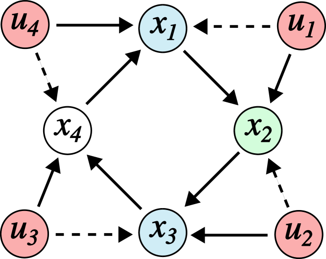
Consider the following system , where , depicted as a network in figure 1:
The dynamics simply permute the state of four nodes, and measures the state of nodes and , and if . The inputs may be thought of as edge attacks which could “interfere” with the transmission of information from a given node to the next, by changing the apparent amount of information transmitted. Since in this example, the system is not classically left invertible, but here we will suppose that inputs are -sparse. We will demonstrate that the system is not left -sparse invertible with but is left -sparse invertible when , using propositions 3, 4, and 6.
IV-A , Geometric Characterization
Consider the state . By choosing , . Hence, for all , . Likewise, implies , and a choice of results in . So . However, suppose , then no 1-sparse input can result in , but there does exist a 2-sparse input satisfying this requirement. It follows that and .
Observe that , so . In particular, it contains , which is also contained in . Therefore, by proposition 3, is not -sparse invertible.
IV-B , Rank-Based Characterization
Consider that the matrix
| (15) |
satisfies for any . Since , for any other , , so by proposition 4, is left -sparse invertible with delay 1.
IV-C , Spectral Characterization
Consider the strongly -sparse reachable point . The input results in . Let denote a basis for the subspace of to which belongs, we may write . Setting , we have that
| (16) |
By proposition 6, we may conclude that is not left -sparse invertible.
V Discussion
As a collection of necessary and sufficient conditions for the well-posedness of sparse recovery problems, this work deals with conditions that are by their nature computationally hard [23]. However, they provide a natural scaffolding to deal with sparse inversion problems, and in particular for structured and networked systems, where the inherent delay of a system can be generically nontrivial [22]. We expect that, as in the case of the classical relaxation for sparse recovery, optimal and computationally tractable implementations will arise as relaxations of appropriate combinatorial problems in this setting. The following are interesting future directions and applications of our results:
V-A Bounding constants associated with
The difficulty of verifying the conditions in this work is determined by the size of and their indices . We expect that the magnitude of implied by the proof of proposition 1 is a dramatic overshoot in most cases, and future work should seek to establish general bounds.
V-B Connections to Inversion of Switched Systems
One may formally identify linear systems with sparse inputs with a class of switched systems: consider the support to be an unknown switching signal determining the time varying system . We expect that our results on invertibility may therefore be generalized to a class of switched systems, where switching is restricted to the and matrices.
V-C Generalization to Inputs taking values in Subspace Arrangements
All of our results use properties of sparsity which are also features of subspace arrangements generally. We therefore expect immediate generalization to the setting where , and is a finite subspace arrangement. In the case that is a subspace arrangement that is not finite–for example, taken to be the set of rank 1 matrices–generalization is less clear, and is an interesting direction for future work. Such results could
V-D Strong Observability and Unknown Input Observers
Strong observability, the ability to recover the initial state in finite time in the presence of unknown inputs, may be geometrically characterized for linear systems as having a trivial weakly unobservable subspace. Analogously, is necessary and sufficient for initial state recovery in the presence of unknown -sparse inputs. Exploring a characterization of strong detectability, known to be a necessary and sufficient condition for the existence of an unknown input observer for linear systems, is a direction of interest in the sparse case.
V-E Right Invertibility
Right invertibility is formally the ability to construct an input and initial condition which produces any desired output. Due to space constraints, we have restricted our exposition in this work to focus on left invertibility; however, we expect similar arguments to lead to characterizations of right invertibility in the sparse input setting.
VI Conclusions
In this work, we have established the first necessary and sufficient conditions for the left invertibility of linear systems with sparse inputs. Leveraging properties of the novel weakly unobservable and strongly reachable subspace arrangements, these characterizations echo the fundamental characterizations of invertibility for standard linear systems. We expect that these characterizations will lead to the generalization of a variety of techniques for inversion of linear systems, and enable a systematic approach to related problems in sparse control.
References
- [1] M. Sain and J. Massey, “Invertibility of linear time-invariant dynamical systems,” IEEE Transactions on automatic control, vol. 14, no. 2, pp. 141–149, 1969.
- [2] R. M. Hirschorn, “Invertibility of nonlinear control systems,” SIAM Journal on Control and Optimization, vol. 17, no. 2, pp. 289–297, 1979.
- [3] B. Liu and J. Si, “Fault detection and isolation for linear time-invariant systems,” in Proceedings of 1994 33rd IEEE Conference on Decision and Control, vol. 3, 1994, pp. 3048–3053 vol.3.
- [4] A. Edelmayer, J. Bokor, Z. Szabó, and F. Szigeti, “Input reconstruction by means of system inversion: A geometric approach to fault detection and isolation in nonlinear systems,” International Journal of Applied Mathematics and Computer Science, vol. 14, no. 2, pp. 189–199, 2004.
- [5] M. Hou and R. J. Patton, “Input observability and input reconstruction,” Automatica, vol. 34, no. 6, pp. 789–794, 1998.
- [6] A. Martinelli, “Nonlinear unknown input observability: Extension of the observability rank condition,” IEEE Transactions on Automatic Control, vol. 64, no. 1, pp. 222–237, 2019.
- [7] P. Sannuti and A. Saberi, “Special coordinate basis for multivariable linear systems—finite and infinite zero structure, squaring down and decoupling,” International Journal of Control, vol. 45, no. 5, pp. 1655–1704, 1987.
- [8] M. Tranninger, H. Niederwieser, R. Seeber, and M. Horn, “Unknown input observer design for linear time-invariant systems—a unifying framework,” International Journal of Robust and Nonlinear Control, vol. 33, no. 15, pp. 8911–8934, 2023.
- [9] A. Ansari and D. S. Bernstein, “Deadbeat unknown-input state estimation and input reconstruction for linear discrete-time systems,” Automatica, vol. 103, pp. 11–19, 2019.
- [10] H. L. Trentelman, A. A. Stoorvogel, M. Hautus, and L. Dewell, “Control theory for linear systems,” Appl. Mech. Rev., vol. 55, no. 5, pp. B87–B87, 2002.
- [11] P. Moylan, “Stable inversion of linear systems,” IEEE Transactions on Automatic Control, vol. 22, no. 1, pp. 74–78, 1977.
- [12] S. Sefati, N. J. Cowan, and R. Vidal, “Linear systems with sparse inputs: Observability and input recovery,” in IEEE American Control Conference (ACC), 2015, pp. 5251–5257.
- [13] K. Poe, E. Mallada, and R. Vidal, “Necessary and sufficient conditions for simultaneous state and input recovery of linear systems with sparse inputs by -minimization,” in IEEE Conference on Decision and Control (CDC), 2023, pp. 6499–6506.
- [14] R. K. Chakraborty, G. Joseph, and C. R. Murthy, “Joint state and input estimation for linear dynamical systems with sparse control,” arXiv preprint arXiv:2312.02082, 2023.
- [15] C. Sriram, G. Joseph, and C. R. Murthy, “Control of linear dynamical systems using sparse inputs,” in IEEE International Conference on Acoustics, Speech and Signal Processing (ICASSP), 2020, pp. 5765–5769.
- [16] A. J. Florez and L. F. Giraldo, “Structural sparsity in networked control systems,” IEEE Transactions on Systems, Man, and Cybernetics: Systems, vol. 50, no. 12, pp. 5152–5161, 2020.
- [17] M. Zhang, B. Alenezi, S. Hui, and S. H. Żak, “State estimation of networked control systems corrupted by unknown input and output sparse errors,” in American Control Conference (ACC), 2020, pp. 4393–4398.
- [18] A. S. Charles, A. Balavoine, and C. J. Rozell, “Dynamic filtering of time-varying sparse signals via minimization,” IEEE Transactions on Signal Processing, vol. 64, no. 21, pp. 5644–5656, 2016.
- [19] N. P. Bertrand, A. S. Charles, J. Lee, P. B. Dunn, and C. J. Rozell, “Efficient tracking of sparse signals via an earth mover’s distance dynamics regularizer,” IEEE Signal Processing Letters, vol. 27, pp. 1120–1124, 2020.
- [20] G. Joseph, C. R. Murthy, R. Prasad, and B. D. Rao, “Online recovery of temporally correlated sparse signals using multiple measurement vectors,” in IEEE Global Communications Conference (GLOBECOM), 2015, pp. 1–6.
- [21] G. Joseph and C. R. Murthy, “A noniterative online bayesian algorithm for the recovery of temporally correlated sparse vectors,” IEEE Transactions on Signal Processing, vol. 65, no. 20, pp. 5510–5525, 2017.
- [22] F. Garin, “Generic delay-l left invertibility of structured systems,” IFAC-PapersOnLine, vol. 55, no. 13, pp. 210–215, 2022.
- [23] S. T. McCormick, A combinatorial approach to some sparse matrix problems. Stanford University Stanford, CA, 1983, vol. 83.