Probing Heavy Charged Higgs Boson Using Multivariate Technique at Gamma-Gamma Collider
Abstract
The current study explores the production of charged Higgs particles through photon-photon collisions within the Two Higgs Doublet Model context, including one-loop-level scattering amplitude of Electroweak and QED radiation. The cross-section has been scanned for plane () investigating the process of . Three particular numerical scenarios low-, non-alignment, and short-cascade are employed. Hence using for low- and for non-alignment and short-cascade scenario, the new experimental and theoretical constraints are applied. The decay channels for charged Higgs particles are examined in all the scenarios along with the analysis for cross-sections revealing that at low energy it is consistently higher for all scenarios. However, as increases, it reaches a peak value at 1 TeV for all benchmark scenarios. The branching ratio of the decay channels indicates that for non-alignment, the mode of decay takes control and for short cascade, the prominent decay mode remains , while in the low- the dominant decay channel is of . In our research, we employ contemporary machine-learning methodologies to investigate the production of high-energy Higgs Bosons within a 3TeV Gamma-Gamma collider. We have used multivariate approaches such as Boosted Decision Trees (BDT), LikelihoodD, and Multilayer Perceptron (MLP) to show the observability of heavy-charged Higgs Bosons versus the most significant Standard Model backgrounds. The purity of the signal efficiency and background rejection are measured for each cut value.
pacs:
12.60.Fr, 14.80.FdI Introduction
A neutral Higgs boson was discovered by the ATLAS and CMS collaborations at the Large Hadron Collider (LHC) in 2012 having approximately a mass of 125 GeV and its properties were consistent with the prediction of Standard Model (SM) Higgs atlas2012observation ; cms2012observation ; collaboration2015precise . Within the SM framework, gauge boson acquire their masses due to the Brout–Englert–Higgs mechanism utilizing the concept of electroweak symmetry breaking (EWSB). The SM of particle physics does not provide any indications of charged Higgs bosons. However, theories beyond the SM propose the existence of charged Higgs bosons and are frequently incorporated into theoretical frameworks such as Two-Higgs-Doublet Models (2HDM), supersymmetric models, composite Higgs models grand unified theories, and axion models. Among all these BSM theories, the two Higgs doublet model is very important due to its structural relevance to many new physics models like MSSM arhrib2017prospects ; ross1975neutral , composite Higgs models, axion models veltman1976second ; veltman1977limit . Depending upon the couplings to the quarks, the types of 2HDMs predict different properties and interactions for charged Higgs bosons. A charged Higgs boson would be a more massive counterpart to the SM and bosons, which are carriers of the weak force.
The Higgs sector in 2HDM is extended to incorporate other degrees of freedom that include the prediction of five Higgs candidates of the minimal supersymmetric extension of the SM (MSSM) atlas2015study ; collaborations2015combined . From these five Higgs boson candidates, two are CP even neutral states , , one is CP odd state and the remaining two states charge Higgs states . The discovery of any new scalar Higgs boson either neutral or charged will be a strong hint towards the physics beyond the SM of particle physics and the immediate sign of an extended Higgs sector.
The future and colliders, with high energy and luminosity, offer a great potential for discovering charged Higgs boson. The output rate at a collider could exceed that of collisions at the tree level. In 2HDM, the process has been analyzed at the tree level, while the process was only studied at the Born level with Yukawa corrections hashemi2014charged ; ma1996yukawa . Due to the s-channel contribution the triumphs over the cross-section, so the rate of production of is higher than the . The scattering process of has been studied at the one-loop level.
This paper will focus on the multivariate analysis of charged Higgs boson production at the photon-photon collider at the International Linear Collider (ILC). Three benchmark points are selected for numerical examination, each with a -even scalar mass of and couplings consistent with the known Higgs boson. These points are derived from the “non-alignment”, “low-”, and “short-cascade” scenarios, and have been accurately delineated within the constraints of current experimental data and are fully consistent with theoretical constraints haber2016erratum . The cross-section is scanned for plane , where is for low- and for non-alignment and short-cascade scenarios. Additionally, the polarization effect is also discussed for all scenarios.
II Review of Two Higgs Doublet Model
The two scalar doublets are used to acquire masses for gauge bosons and fermions after having their vacuum expectation values (VEVs). The Lagrangian is given by:
| (1) |
Where is the Lagrangian for two scalar doublets including kinetic term and scalar potential terms. The symmetry is involved to ignore the Flavour Changing Neutral currents (FCNCs), then the transformation for even, , and for odd is . To keep invariant for fermions under -symmetry the fermions are coupled with one scalar field:
| (2) |
In Equation 2 the is either or , so based on the discrete symmetry of fermions the 2HDM is classified into four types called as Type-I, II, III, and IV. The review for this relevant study is discussed here for -conserving 2HDM. If we assume that in the 2HDM the electromagnetic gauge symmetry is present to perform rotation on two doublets for alignment of VEVs of two doublets with and the will occupy one neutral Higgs doublet craig2013searching . The two complex doublets, from SM and from EW symmetry-breaking are used to construct the 2HDM. The scalar potential under invariant gauge group is defined as
| (3) |
In the above Equation 3 the quartic coupling parameters are and the complex two doublets are . Hermiticity of the potential forces to be real while and can be complex. The Paschos-Glashow-Weinberg theorem suggests that a discrete -symmetry can explain certain low-energy observables glashow1977natural ; paschos1977diagonal . Utilizing this symmetry is crucial to effectively prevent any possibility of FCNCs occurring at the tree level. The -symmetry requires that and also . If this is not allowed i.e. is non-zero then the -symmetry is softly broken for the translation of and . The assignments produce four 2HDM-types as mentioned earlier branco2012theory ; gunion2000print . Table 1 demonstrates how fermions bind to each Higgs doublet in the permitted kinds when flavor conservation is naturally observed.
| Type | |||
|---|---|---|---|
| I | |||
| II | |||
| III | |||
| IV |
This work focuses only on Type-I and Type-II 2HDM whereas in Type-I only doublet interacts with both quarks and lepton similarly as SM. In Type-II the couples with d-type quarks and leptons while the with only u-type quarks.
After electroweak symmetry breaking of , the scalar doublet’s neutral components gets VEV to be .
| (4) |
where and are real scalar fields. The quartic coupling parameters and mass terms , are considered as physical masses of with and mixing term . After -symmetry is broken softly the parameter is given by
| (5) |
where the last equality is only for the tree level. By considering and equal to zero concerning -symmetry, , and mixing angle with four Higgs mass is enough to compute a complete model in physical basis. So, with all this, there are seven independent free parameters to explain the Higgs sector in 2HDM. The terms and are given in the form of other parameters:
| (6) |
| (7) |
The phenomenology is dependent upon the mixing angle with angle . In the limit where -even Higgs boson acts like SM Higgs then it approaches the non-alignment limit which is most favored by experimentalists if or . The acts as gauge-phobic such that its coupling with vector bosons is much more suppressed, but when the acts SM-like Higgs boson. For the decoupling limits and so at this limit interacts with SM particles completely appears like the couplings of the SM Higgs boson that contain coupling .
III Constraints from Theory and Experiment
The theoretical restrictions of potential unitarity, stability, and perturbativity compress the parameter space of the scalar 2HDM potential. The vacuum stability of the 2HDM limits the . Specifically, needs to be met for all and directions. As a result, the following criteria are applied to the parameters deshpande1978pattern ; cms2010search
| (8) |
Another set of constraints enforces that the perturbative unitarity needs to be fulfilled
for the scattering of longitudinally polarized gauge and Higgs bosons. Besides, the scalar potential needs to be perturbative by demanding that all quartic coefficients satisfy . The global fit to EW requires to be gfitter2014global . This prevents
substantial mass splitting between Higgs boson in 2HDM and requires that or
.
Aside from the theoretical restrictions mentioned above, 2HDMs have been studied in
previous and continuing experiments, such as direct observations at the LHC or indirect B-physics observables. As a consequence, numerous findings have been amassed since then, and the parameter space of the 2HDM is now constrained by all results
obtained. In the Type-I of 2HDM, the following pseudoscalar Higgs mass regions for for for with have been excluded by the LHC experiment aaboud2018search . Furthermore, the odd Higgs mass is bounded as for aad2015collisions and the mass range with is excluded for the Type-I aad2016measurements .
The mass is constrained by experiments at the LHC and prior colliders, as well as B-physics observables. The BR() measurement limits the charged Higgs mass in Type-II and IV 2HDM with for misiak2015updated ; misiak2017weak . On the other hand, the bound is significantly lower in Type-I and III of 2HDM kanemura2015unitarity . With , the in Type-I and III of 2HDM can be as light as enomoto2016flavor ; arhrib2017bosonic while meeting LEP, LHC, and B-physics constraints aad2015search ; khachatryan2015search ; aad2013search ; aleph2013search ; akeroyd2017prospects .
IV Benchmark points scenarios
We have taken three scenarios haber2016erratum : non-alignment, short cascade, and low-. All of these are taken for even scalar of mass and couplings are well arranged with observed Higgs boson. The additional Higgs boson searches leave a considerable portion of their parameter space unconstrained, emphasizing the need for further investigation. Validation of potential stability, perturbativity, and unitarity for each BP was performed using 2HDMC 1.8.0 eriksson20102hdmc .
These benchmark situations, shown in Table 2, are created using a hybrid approach, where the input parameters are specified as with softly broken 2HDM of symmetry, where the are quartic couplings in Higgs basis of (1). The mass of charged Higgs and pseudoscalar Higgs in this basis are obtained as:
| (9) |
| (10) |
In the non-alignment scenario, the lightest even scalar , the discovered Higgs boson is interpreted, with SM-like properties. In an alignment scenario heavy even
could not decay into GB but in a non-alignment scenario it is allowed by present constraints. In this situation to have a must satisfy the constraint, and quartic couplings are set to -2. The and are remain free parameters.
In the short-cascade scenario the SM like is taken exactly to alignment i.e . We considered mass hierarchy such as to decay or which results Higgs-to-Higgs decay in small cascade. The and are remained fixed parameters.
A low scenario is proposed where both even Higgs boson () are light. The heavier one is assumed to be an SM-like Higgs boson, resulting in . The heavier even Higgs coupling to gauge bosons is proportional to . Because , the couplings of lighter even scalars to vector bosons must have been strongly suppressed
to comply with direct search limits, forcing . The parameter space for is constrained by searches at the LHC, which leads to an upper constraint on .
| Scenario |
[GeV] |
[GeV] |
|||||
|---|---|---|---|---|---|---|---|
| BP-1 | 125 | 150…600 | 0.1 | -2 | -2 | 0 | 1…20 |
| BP-2 | 125 | 250…500 | 0 | -1 | 1 | -1 | 2 |
| BP-3 | 125 | 250…500 | 0 | 2 | 0 | -1 | 2 |
| BP-4 | 65…120 | 125 | 1.0 | -5 | -5 | 0 | 1.5 |
The mass hierarchy is considered for these benchmark points along with the type of the 2HDMs, shown in Table 3. In Table 2, and .
| Scenarios | BP’s | 2HDM-Type | Mass Hierarchy |
|---|---|---|---|
| Non-alignment | BP-1 | I | |
| Short Cascade | BP-2 | I | |
| Short Cascade | BP-3 | I | |
| Low- | BP-4 | II |
V The leading order cross-section of charged Higgs production
Analytical formulations of the cross-section of the collider for charged Higgs pair generation are presented in this section. The process used in this paper is given as:
| (11) |
where represent the four momenta. There are three different diagrams at the tree level that are topologically distinct because of photon coupling as shown in Figure 1. The total Feynman amplitude is given by:
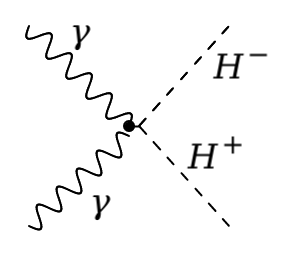
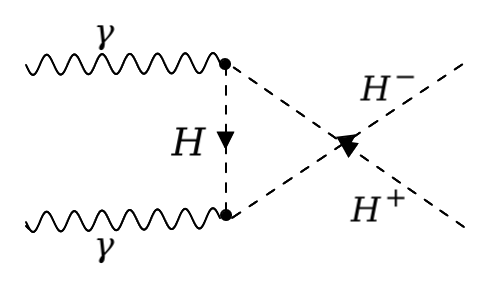
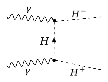
| (12) |
where and are amplitudes of quartic couplings, t-channel, and u-channel Feynman diagrams respectively. The relations for these channels are given as follows:
| (13) |
| (14) |
| (15) |
where the Mandelstam variables are represented by and . After calculating the square of the total amplitude and summing up the polarization vectors, the expression becomes:
| (16) |
The scattering amplitude is calculated numerically in the center of the mass frame, where the four-momentum and scattering angle are indicated by . In the center of mass energy, the energy and momentum of incoming and outgoing particles are:
| (17) |
| (18) |
| (19) |
| (20) |
| (21) |
where is the mass of relevant particles. The cross-section is calculated by taking the flux of incoming particles and the integral over the phase space of outgoing particles is given by:
| (22) |
In above expression the is the Kllen function relevant to phase space of outgoing . The total integrated cross section for -collider could be calculated by:
| (23) |
where and are the C.M enrgy in -collider and subprocess of , respectively. The value of represents the minimum amount of energy needed to generate a pair of charged Higgs particles and is given by , where the is 0.83 telnov1990problems . The distribution function of the photon luminosity is:
| (24) |
The energy spectrum of Compton back-scattered photons, , is characterized by the electron beam’s longitudinal momentum telnov1990problems .
VI NUMERICAL RESULTS AND DISCUSSIONS
The numerical results of generating charged Higgs boson via photon-photon collisions are thoroughly examined in the context of 2HDM including QED radiations. Cross sections at the tree level are calculated numerically for each benchmark scenario as a function of the C.M energy and the Higgs boson mass. Polarization distributions are presented to improve the production rate by considering longitudinal polarizations of initial beams. Decay pathways of the charged Higgs boson are under study for relevant scenarios.
In our work, for analytical and numerical evaluation we have used MadGraph5 v3.4.2 alwall2011madgraph for the calculations of the cross-sections, the 2HDMC 1.8.0 rathsman20112hdmc for the branching ratio and total decay width. The GnuPlot williams2012gnuplot is used for the graphical plotting.
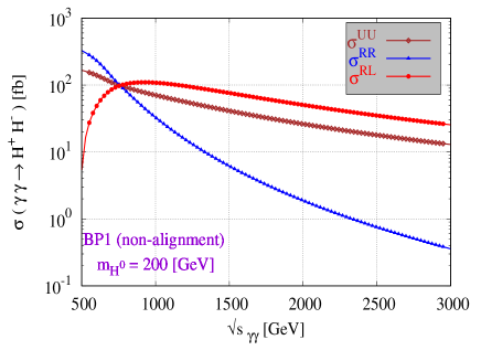
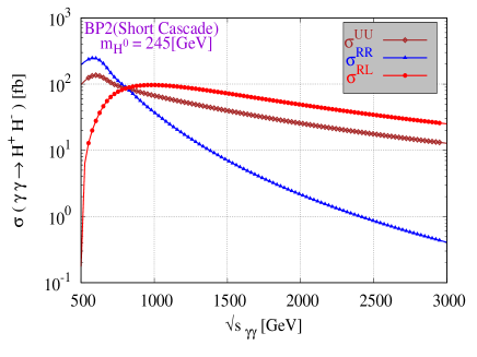
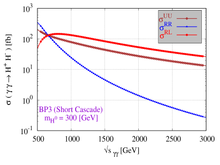
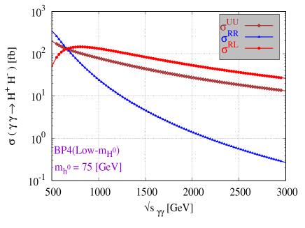
As in Figure 2 the cross-section for the process is shown for the C.M energy of for three types of polarization; right handed (), oppositely-polarized () and unpolarized beam . The cross-section is the same for the polarization modes of . In Figure 2 it can be seen that the cross-section is higher for and for low and gradually decreases. But for the mode of polarization, the cross-section reaches a peak value and then gradually decreases. As we can see the cross-section is not enhanced for and at higher energies but it does only for .
In Figure 3 for both BPs, the cross-section changes slowly with the mass of and because of the small range of charged Higgs mass. For both and modes of polarization the cross-section decreases with C.M energy and for mode it reaches a peak value and then decreases. The cross-section decreases for when .
VII decays of charged Higgs Boson
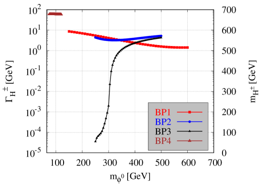
The probability that a particular particle will decay per unit time is called decay width. While it is impossible to predict the lifespan of a single particle, a statistical distribution can be determined for a large sample, for this purpose the decay width is used. In this section, we will study the final decay products of the charged Higgs bosons created in all scenarios. To investigate the process in a collider, we must first identify all potentially charged Higgs products. The total decay widths of the charged Higgs boson versus the mass of Higgs or are plotted for all BPs.
The total rate of decay per unit time is the sum of all individual decay rates,
.
In our system of natural units, the dimension of is equivalent to mass (or energy) as it is the inverse of time. As expected, the mass of the charged Higgs boson increases with increasing neutral Higgs mass under all circumstances. The decay widths are highly sensitive to the mass hierarchy and mass splitting. Shrinking of the decay width is observed when , the mass splitting is minimal, as shown in Figure 4. The decay width for BP-1 decreases from to when the goes from to . For BP-2, the decay width increases from to for in the range of . The for BP-3 increases from to when runs from to . For the last BP-4, the decay width decreases from to for change of from to .
The BR (or branching fraction) is the proportional frequency of a particular decay mode. The BR is the decay rate to the specific mode i.e. relative to the total decay rate.
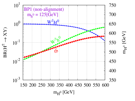
Here is the total decay width and is the partial decay width i.e. decay width of an individual particle. We showed the dominant modes of BR for as function of and , for all scenarios. The channel is the primary decay mode for in BP-1, as shown in Figure 5. The sub-dominant channels are as follows: and for charged Higgs for BP-1, other suppressed channels are and for range . The mode of decay takes control when decreases at larger values of . So for range rises from 1.2 to of . The process to is also another dominant decay mode with BR of 88.7 to 50.2% and with hadronic decay of has 12-jets in the final state.
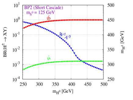
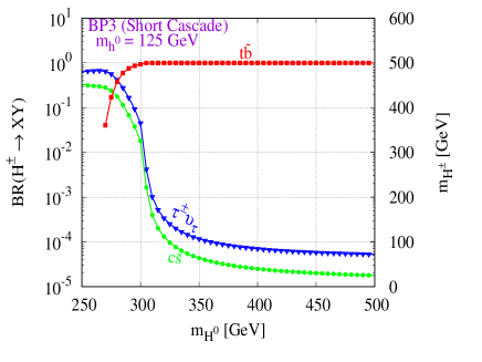
In the BP-2 and BP-3 as shown in Figure 5 and Figure 6 respectively, as the BR of 100% prominent decay mode is . The suppressed decay modes of are for and in both BP-2 and BP-3; the quark decay is an ideal for the reconstruction of the process at . So for process gives trace at the detector which can be tagged with 8-jets and 2-b-tagged jets.
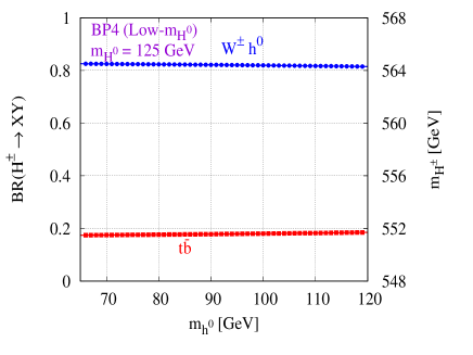
For BP-4, shown in Figure 6, for a range of the dominant channel is because for it leads to 100%. 4-jets and 4-b-tagged jets can be used to tag the process.
VIII Multivariate Analysis for charged Higgs production
An integrated ROOT framework for parallel running and computation of several multivariate categorization algorithms is called the “Toolkit for Multivariate Analysis” brun1997root , which categorizes using two sorts of events: signal and background. TMVA especially has many applications in high energy physics for the complex multiparticle final state. To train the classifiers, a set of events with well-defined event types is inserted into the Factory. The event samples for signal and background can either be read using a tree-like structure or a plain text file using a defined structure. All variables that are supposed to separate signal and background events must be known by the Factory. Cuts are applied on signal and background trees separately.
We represent three classifiers in our work; Boosted Decision Tree (BDT), LikelihoodD (Decorrelation), and MLP. In BDT a selection Tree is a tree-like structure that illustrates the different outcomes of a choice using a branching mechanism. An event is categorized as either a signal or a background event by passing or failing to pass a condition (cut) on a certain node until a choice is reached. The “root node” of the decision tree is used to find these cuts. The node-splitting process concludes when the BDT algorithm specifies minimal events (NEventsMin).

| MVA Classifier | AUC (with cut) | AUC (without cut) |
|---|---|---|
| MLP | 0.958 | 0.922 |
| BDT | 0.957 | 0.925 |
| LikelihoodD | 0.941 | 0.896 |
The final nodes (leaves) are classified according to their “purity” (p). The value for signal or background (usually for signal and 0 or for background) depends on whether p is greater than or less than the stated number, e.g. +1 if and if coadou2022boosted . To differentiate between the background class and signal, a labeling process is carried out. All occurrences with a classifier output are labeled as a signal, while the rest are classified as background. The purity of the signal efficiency , and background rejection () are evaluated for each cut value of speckmayer2010toolkit . ADA-Boost algorithm re-weights every misclassified event candidate. The new candidate weight consists of the one used in the former tree multiplied by , where is the misclassification error. This leads to an increase in the weight and therefore an increase in the candidate’s importance when searching for the best separation values. The weights of each new tree are based on the ones of its predecessor meir2003introduction .
An Artificial Neural Network (ANN) comprises linked neurons, each with its weight. To speed up the processing, a reduced layout can be used as well, the so-called multilayer perception (MLP). The network consists of three kinds of layers. The input layer, consisting of neurons and a bias neuron, many deep layers containing a user-specified number of neurons (set in the option HiddenLayers) plus a bias node, and an output layer and each of the connection between two neurons carries a weight.
For event , the likelihood ratio is defined by
| (25) |
where the likelihood of a candidate to be signal/background may be determined using the following formula
| (26) |
where is the PDF for the th input variable . The PDFs are normalized to one for all :
| (27) |
The projective likelihood classifier has a major drawback in that it does not use correlation among the discriminating input variables. In the realistic approach, it does not provide an accurate analysis and leads to performance loss. Even other classifiers underperform in the presence of variable correlation. Linear Correlation was used to quantify the training sample by obtaining the square root of the covariant matrix. The square root of the matrix is , which when multiplied by itself yields . As a result, TMVA employs diagonalization of the (symmetric) covariance matrix provided by:
| (28) |
is the diagonal matrix, while denotes the symmetric matrix. The linear decorrelation is calculated by multiplying the starting variable by the inverse of .
| (29) |
Only linearly coupled and Gaussian distributed variables have full decorrelation. In this work, the signal and background events are taken to be 50000 with applied cuts:
| MVA Classifier |
Signal Significance
(with cuts) |
Signal Significance
(without cuts) |
|---|---|---|
| MLP | 201.44 | 192.187 |
| LikelihoodD | 198.658 | 188.409 |
| BDT | 201.532 | 193.05 |
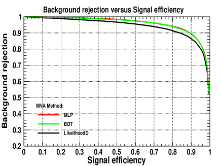
The curve of background rejection against signal efficiency provides a reasonable estimate of a classifier’s performance. A classifier’s performance is measured by the area under the signal efficiency versus the background rejection curve, so the bigger the area, the better a classifier’s predicted separation power, as shown in Figure 7. The values of area under the curve (AUC) for Figure 7. Table 4 shows that the best classifier among all is the MLP and BDT, improved after applying cuts and gave the largest area under the curve.
We used 800 trees to improve the BDT’s performance, with node splitting at event threshold. Max tree depth set at 3. Trained using Adaptive Boost with a learning rate of parent node and the sum of the indices of the two daughter nodes are compared to optimize the cut value on the variable in a node. For the separation index, we use the Gini Index. Finally, the variable’s range is evenly graded into 20 cells. The signal values are taken to be 1 and background values approach to 0.
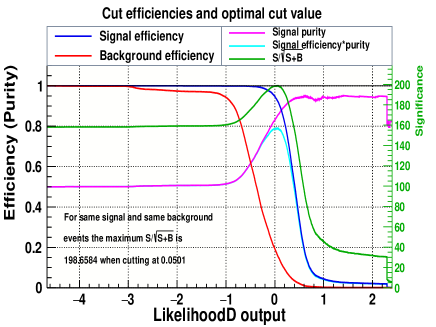
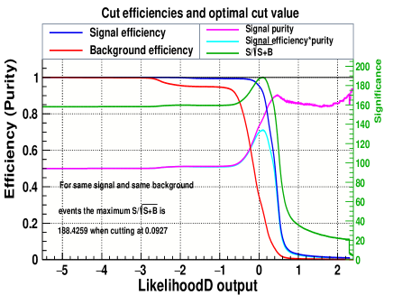
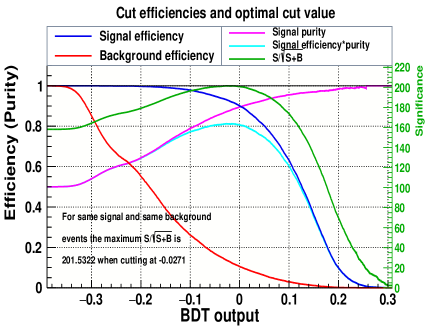
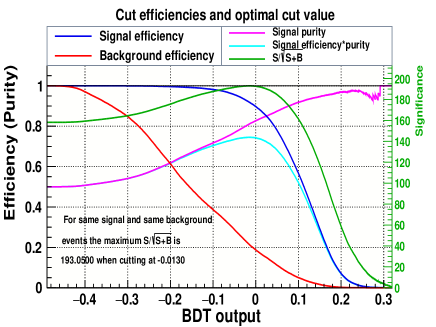
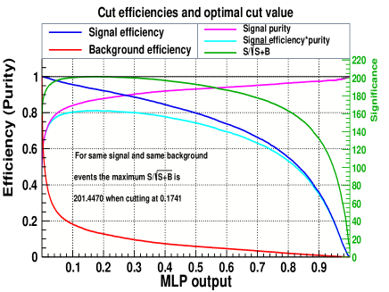
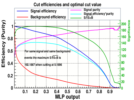
Figure 8 depicts that the signal significance, , of the classifier, is improved by applying cuts with an optimal cut of -0.0271. Similarly, Figure 9 shows the best classifier that is improved by applying cuts with an optimal cut value of 0.1741, and the signal efficiency is also higher than without applied cuts. The LikelihoodD signal significance is shown in Figure 10, has been improved by applied cuts with the optimal cut of 0.0501.
IX conclusion
The simplest extension of SM is 2HDM containing charged Higgs Boson and the exact measurement of its nature corresponding model parameters are crucial for the discovery. The pair production is one of the best channels that provided the observable signal in the vast range of parameters in 2HDM.
The generation rates of incoming beams are investigated in various polarization collision patterns. The cross-section can be increased twice by oppositely polarized beams of photons at high energies and right-handed polarized beams of photons at low energies as shown in the figures of the cross-section. For BP-1 at the the fb , for fb and for fb. For BP-2 the cross section for fb, fb and for fb at the center of mass energy . The cross section at for BP-3 for different polarizations are fb, fb and fb respectively. The Low- scenario for BP-4 the cross section for polarized beams are fb, fb and for fb at respectively. So we concluded that for all BP’s, the cross-section is low at high energy for and polarized beams of photons, while high for at high energy.
For each scenario, the charged Higgs Boson reconstruction has been provided, and its prominent decay modes have been examined. The branching ratio of the decay channel for non-alignment, the bosonic decay channel is the dominant while in the low scenarios the bosonic decay of is dominant rises to . The dominant decay channel in a short-cascade scenario is that concludes the decay is the ideal candidate for the reconstruction of the process. Limited phase space and alignment constraints restrict bosonic decay channels.
Our Machine Learning models for Multivariate Analysis results are improved by applying cuts. The signal efficiency and background rejection are increased when cuts are applied to the MLP, BDT, and LikelihoodD classifiers. The area under the curve (AUC) is increased for MLP to , for BDT increased to , and the LikelihoodD increased up to which shows that the LikelihoodD is the more efficient classifier for signal efficiency and background rejection. The signal significance is increased for MLP to , for the BDT increased to , and for LikelihooD, it is increased to by applying cuts. The significance values obtained with cuts demonstrate how well these models can separate charged Higgs production-related background events from signal occurrences. These cuts most likely aid in lowering background noise, enhancing overall performance, and separating signal events associated with charged Higgs generation. This consistency upholds the validity of the selected machine-learning approaches and increases trust in the outcomes.
X Acknowledgements
We gratefully acknowledge support from the Simons Foundation and member institutions. The current submitted version of the manuscript is available on the arXiv pre-prints home page
XI Statements and Declarations
Funding
The authors declare that no funds, grants, or other support were received during the preparation of this manuscript.
Competing Interests
The authors have no relevant financial or non-financial interests to disclose.
Availability of data and materials
Data sharing does not apply to this article as no datasets were generated or analyzed during the current study.
References
- (1) Observation of a new particle in the search for the Standard Model Higgs boson with the ATLAS detector at the LHC, ATLAS, Collaboration, arXiv preprint arXiv:1207.7214, (2012)
- (2) Observation of a new boson at a mass of 125 GeV with the CMS experiment at the LHC, CMS Collaboration, arXiv preprint arXiv:1207.7235, (2012)
- (3) Precise determination of the mass of the Higgs boson and tests of compatibility of its couplings with the standard model predictions using proton collisions at 7 and 8 TeV, Collaboration, CMS, Eur. Phys. J. C, (2015)
- (4) Prospects for charged Higgs searches at the LHC., Arhrib, A and Hernandez-Sanchez, J and Mahmoudi, F and Santos, R and Akeroyd, A and Moretti, S and Yagyu, K and Yildirim, E and Khater, W and Krawczyk, M and others, European Physical Journal C–Particles & Fields, (2017)
- (5) Neutral currents and the Higgs mechanism, Ross, DA and Veltman, M, Nuclear Physics B, (1975)
- (6) Second threshold in weak interactions, Veltman, MJG, Acta Phys. Pol. B, (1976)
- (7) Limit on mass differences in the Weinberg model, Veltman, M, Nuclear Physics B, (1977)
- (8) Study of production and Higgs boson couplings using decays with the ATLAS detector, ATLAS collaboration and others, arXiv preprint arXiv:1506.06641, (2015)
- (9) Combined Measurement of the Higgs Boson Mass in pp Collisions at 7 and 8 TeV with the ATLAS and CMS Experiments, Collaborations, CMS, and others, arXiv preprint arXiv:1503.07589, (2015)
- (10) Charged Higgs pair production in a general two Higgs doublet model at and linear colliders, author=Hashemi, Majid, Communications in Theoretical Physics, (2014)
- (11) Yukawa corrections to charged Higgs-boson pair production in photon-photon collisions, Ma, Wen-Gan and Li, Chong Sheng and Liang, Han, Physical Review D, (1996)
- (12) Erratum to New LHC benchmarks for the CP-conserving two-Higgs-doublet model, Haber, Howard E and Stål, Oscar, The European Physical Journal C, (2016)
- (13) Searching for signs of the second Higgs doublet, Craig, Nathaniel and Galloway, Jamison and Thomas, Scott, arXiv preprint arXiv:1305.2424, (2013)
- (14) Natural conservation laws for neutral currents, Glashow, Sheldon L, and Weinberg, Steven, Physical Review D, (1977)
- (15) Diagonal neutral currents, Paschos, Emmanuel A, Physical Review D, (1977)
- (16) Theory and phenomenology of two-Higgs-doublet models, Branco, Gustavo Castelo and Ferreira, PM and Lavoura, L and Rebelo, MN and Sher, Marc and Silva, Joao P, Physics reports, (2012)
- (17) PRINT-86-1324 (UC, DAVIS); JF Gunion, HE Haber, GL Kane and S. Dawson, Gunion, John F and Kayser, B, and Mohapatra, RN and Deshpande, NG and Grifols, J and Mendez, A and Olness, FI and Pal, PB, Front. Phys, (2000)
- (18) Pattern of symmetry breaking with two Higgs doublets, Deshpande, Nilendra G and Ma, Ernest, Physical Review D, (1978)
- (19) Search for microscopic black hole signatures at the Large Hadron Collider, CMS collaboration and others, arXiv preprint arXiv:1012.3375, (2010)
- (20) The global electroweak fit at NNLO and prospects for the LHC and ILC, Gfitter Group and Baak, M, and Cúth, J and Haller, J and Hoecker, A and Kogler, Roman and Mönig, K and Schott, M and Stelzer, J, The European Physical Journal C, (2014)
- (21) Search for heavy ZZ resonances in the final states using proton-proton collisions at TeV with the ATLAS detector, Aaboud, M and Aad, G and Abbott, B and Abeloos, B and Abidi, SH and AbouZeid, OS and Abraham, NL and Abramowicz, H and Abreu, H and Abreu, R and others, The European Physical Journal. C, Particles, and fields, (2018)
- (22) collisions at TeV with the ATLAS detector. Physics Letters B, 744, pp. 163-183. Copyright© 2015 CERN, for the ATLAS Collaboration., Aad, G, and others, Physics Letters B, (2015)
- (23) Measurements of the Higgs boson production and decay rates and coupling strengths using pp collision data at and 8 TeV in the ATLAS experiment, Aad, Georges and Abbott, Brad and Abdallah, Jalal, and Aben, R and Abolins, M and AbouZeid, OS and Abramowicz, H and Abreu, H and Abreu, R and Abulaiti, Y and others, The European Physical Journal C, (2016)
- (24) Updated next-to-next-to-leading-order QCD predictions for the weak radiative B-meson decays, Misiak, M and Asatrian, HM, Boughezal, Radja and Czakon, M and Ewerth, T and Ferroglia, A. and Fiedler, P. and Gambino, Paolo and Greub, Christoph and Haisch, U, and others, Physical review letters, (2015)
- (25) Weak radiative decays of the B meson and bounds on in the Two-Higgs-Doublet Model, Misiak, Mikołaj and Steinhauser, Matthias, The European Physical Journal C, (2017)
- (26) Unitarity bound in the most general two Higgs doublet model, Kanemura, Shinya and Yagyu, Kei, Physics Letters B, (2015)
- (27) Flavor constraints on the two Higgs doublet models of symmetric and aligned types, Enomoto, Tetsuya and Watanabe, Ryoutaro, Journal of High Energy Physics, (2016)
- (28) Bosonic decays of charged Higgs bosons in a 2HDM type-I, Arhrib, Abdesslam and Benbrik, Rachid and Moretti, Stefano, The European Physical Journal C, (2017)
- (29) Search for charged Higgs bosons decaying via in fully hadronic final states using pp collision data at s = 8 TeV with the ATLAS detector, Aad, Georges Abbott, B. and Abdallah, J and Abdel Khalek, S and Aben, R. and Abi, B. and Abolins, M and AbouZeid, OS and Abramowicz, H and Abreu, H and others, Journal of High Energy Physics, (2015)
- (30) Search for a charged Higgs boson in pp collisions at = 8 TeV, Khachatryan, Vardan and Sirunyan, Albert M and Tumasyan, Armen and Adam, Wolfgang and Asilar, E and Bergauer, Thomas and Brandstetter, Johannes and Brondolin, Erica and Dragicevic, Marko and Erö, Janos and others, Journal of High Energy Physics, (2015)
- (31) Search for a light-charged Higgs boson in the decay channel H+-GT c (s) over-bar in t (t) over-bar events using pp collisions at TeV with the ATLAS detector, Aad, G and Borjanović, Iris and Božović-Jelisavčić, Ivanka and Ćirković, Predrag and Agatonović-Jovin, Tatjana and Krstić, Jelena and Mamužić, Judita and Popović, DS and Sijackii, Dj and Simić, Lj and others, European Physical Journal C. Particles and Fields, (2013)
- (32) Search for charged Higgs bosons: combined results using LEP data, ALEPH Collaboration, DELPHI Collaboration, L3 Collaboration, OPAL Collaboration, and LEP working group for Higgs boson searches, The European Physical Journal C, (2013)
- (33) Prospects for charged Higgs searches at the LHC, Akeroyd, AG and Aoki, M and Arhrib, A and Basso, L and Ginzburg, IF and Guedes, R and Hernandez-Sanchez, J and Huitu, K and Hurth, T and Kadastik, M and others, The European Physical Journal C, (2017)
- (34) 2HDMC–two-Higgs-doublet model calculator, Eriksson, David and Rathsman, Johan and Stål, Oscar, Computer Physics Communications, (2010)
- (35) Problems in obtaining and e colliding beams at linear colliders, Telnov, Valery I, Nuclear Instruments and Methods in Physics Research Section A: Accelerators, Spectrometers, Detectors and Associated Equipment, (1990)
- (36) MadGraph 5: going beyond, Alwall, Johan and Herquet, Michel and Maltoni, Fabio and Mattelaer, Olivier and Stelzer, Tim, Journal of High Energy Physics, (2011)
- (37) 2HDMC-a two Higgs doublet model calculator, Rathsman, Johan and Stål, Oscar, arXiv preprint arXiv:1104.5563, (2011)
- (38) gnuplot 4.6, Williams, Thomas and Kelley, Colin and Bröker, Hans-Bernhard and Campbell, John and Cunningham, Robert and Denholm, David and Elber, Gershon and Fearick, Roger and Grammes, Carsten and Hart, Lucas and others, An Interactive Plotting Program, (2012)
- (39) ROOT—An object-oriented data analysis framework, Brun, Rene and Rademakers, Fons, Nuclear instruments and methods in physics research section A: accelerators, spectrometers, detectors and associated equipment, 1997
- (40) Boosted decision trees, Coadou, Yann, Artificial Intelligence for High Energy Physics, (2022)
- (41) The toolkit for multivariate data analysis, TMVA 4, Speckmayer, P, and Höcker, A and Stelzer, J and Voss, H, Journal of Physics: Conference Series, (2010)
- (42) An introduction to boosting and leveraging, Meir, Ron and Rätsch, Gunnar, Advanced Lectures on Machine Learning: Machine Learning Summer School 2002 Canberra, Australia, February 11–22, 2002 Revised Lectures, (2003)