A reanalysis of the LHS 1140 b atmosphere observed with the Hubble Space Telescope
Abstract
The super-Earth LHS 1140 b is an interesting target for atmospheric observations since it is close to the habitable zone of its star and falls in the gap of the radius distribution of small exoplanets, in the region thought to correspond to the transition between planets with and without atmospheres. Observations of the primary transit with WFC3 on board of the Hubble Space Telescope (HST) revealed a modulation in the planet transmission spectrum compatible with the presence of water; however this modulation may be also due to stellar activity-related phenomena. Here we present a detailed analysis of the WFC3/HST observations to probe the nature of this modulation and to understand if it can be attributable to the presence of unocculted spots on the stellar surface. Our analysis strongly suggests that LHS1140 is a rather quiet star with subsolar [Fe/H] and enriched in elements. Therefore, we rule out the possibility that the planetary spectrum is affected by the presence of spots and faculae. This analysis shows the importance of a proper modelling of the stellar spectrum when analyzing transit observations. Finally, we modelled the planetary atmosphere of LHS1140 b to retrieve its atmospheric composition. However, the low resolution and the narrow spectral range of HST observations prevented us from definitively determining whether the spectral features are attributable to the presence of water or of other molecules in the planetary atmosphere.
keywords:
stars: individual: LHS 1140 – stars: activity – stars: abundances – stars: chemically peculiar – exoplanets – planets and satellites: atmospheres1 Introduction
Nowadays the study of exoplanets and their atmosphere is a leading topic of astronomical research. The main method to study this kind of targets is the transit method, both using photometry and spectroscopy. Specifically, in-transit spectroscopic observations are fundamental to study the atmosphere of exoplanets. The extraction of the planetary spectrum from the transit observations is based on the assumption of a uniform and quiet stellar surface, thus reducing the transit to a purely geometrical effect, but this is not the case for active stars. In fact, the stellar surface of active stars presents active regions which bias the correct derivation of both stellar and planetary parameters, including convection-related phenomena, such as granulation and pulsations (e.g. Berdyugina, 2005), and magnetic activity-related phenomena, such as spots (Solanki, 2003; Ballerini et al., 2012), faculae and flares (e.g. Ballerini et al., 2012). Due to their lower temperature, star spots have a spectrum distinct from that of the surrounding photosphere, with greater contrast at shorter wavelengths. This chromatic dependence changes the stellar spectrum and may distort the entire transmission spectrum of the transiting planet if the distortion is large enough, and may also mimic a planetary atmosphere even if there is none. Therefore, the presence of spots may hamper the extraction of the final transmission spectrum of the planetary atmosphere, for both photometric and spectroscopic observations (e.g. Pont et al., 2008; Czesla et al., 2009; Sing et al., 2009, 2011a, 2011b; Agol et al., 2010; Berta et al., 2011; Désert et al., 2011; Ballerini et al., 2012; Micela, 2015; Scandariato & Micela, 2015). The existence of activity-related “pseudo”-transmission effects is well known and has been discussed, e.g., in Salz et al. (2018), in the context of high-resolution atomic lines. They show that stellar activity related pseudo-signals mix with and confuse the planetary atmospheric absorption signal. Without an accurate analysis of stellar activity the atmospheric analysis remains often uncertain. A number of methods to extract the planetary spectrum taking into account the stellar activity have been proposed in literature (Czesla et al., 2009; Sing et al., 2011b; Ballerini et al., 2012; Micela, 2015; Cracchiolo et al., 2021a, b; Thompson et al., 2023).
On the other hand, the stellar spectrum depends on the stellar metallicity (Z) and the rate of elements (C, O, Ne, Mg, Si, S, Ar and Ca) in the stellar atmosphere can affect deeply the stellar spectrum leading to a wrong interpretation of the planetary spectrum if not correctly accounted for. So, anticipating one of the results of this work, a proper modelling of the stellar spectrum is mandatory in order to properly characterize the planetary atmosphere.
Today, many space missions, currently in flight like JWST (James Webb Space Telescope, Greene et al., 2016; Gardner et al., 2006) or in the development stage, e.g. ARIEL (Atmospheric Remote-Sensing Infrared Exoplanet Large-survey, Tinetti et al., 2018), aim at observing the extrasolar planets to understand their chemical and physical properties through their atmospheres; therefore, in order to achieve this goal, we need to improve our ability to remove chromatic distortions caused by the star.
In this work we analyzed the case of LHS 1140 b to understand how our knowledge of the host star might impact the extraction of the planetary signal and, hence, the retrieval of its atmospheric composition.
With an equilibrium temperature of about , LHS 1140 b is situated close to the habitable zone (HZ) of its star (Dittmann et al., 2017; Kane, 2018; Cadieux et al., 2023), where the existence of liquid water on the planet surface is possible. Recent ground-based observations are not precise enough to constrain atmospheric scenarios (Diamond-Lowe et al., 2020). However, Edwards et al. (2021) using transit observations from Hubble Space Telescope (HST) Wide Field Camera 3 (WFC3) found a modulation in the transit depth of LHS 1140 b over the wavelength range. The authors investigated this modulation, both evaluating multiple atmospheric scenarios to fit the data (trace of in the atmosphere, a moist atmosphere and an atmosphere with and also enriched with ) and investigating the possibility of contamination from stellar activity, specifically due to the presence of stellar spots.
In this paper, we aim to further evaluate the spectral contamination due to the stellar activity adopting the approach of Cracchiolo et al. (2021b) in order to better understand the nature of this system. We analyzed the WFC3/HST observations of LHS 1140 b to understand if this modulation is attributable to the presence of water in the planetary atmosphere or is an artifact due to the presence of spots on the stellar surface.
This paper is organized as follows: in Section 2 we shortly describe the LHS 1140 system and in Section 3 we explain the reduction pipeline that we used to analyze HST data. In Section 4 we derived the temperature and composition of the star from the out-of-transit observation. Section 5 investigates the possibility of stellar activity on this star, while Section 6 explores a discussion on its potential stellar population. Finally, in Section 7, we examine the implications of the stellar composition on the study of LHS 1140b.
2 LHS 1140 b
LHS 1140 is a M4.5-type star (mV = 14.5 Zacharias et al., 2013), located in the costellation of the Whale, at a distance of at () pc (Dittmann et al., 2017; Gaia Collaboration et al., 2023) from the solar system.
It has a surface temperature of K (Cadieux et al., 2023) while Ment et al. (2019) estimated a value of K. The star has a mass of and a radius of (Cadieux et al., 2023).
In April 2017, the exoplanet LHS 1140 b was discovered, orbiting at from its star with a period of (Gomes & Ferraz-Mello, 2020; Cadieux et al., 2023). Its radius is , as derived by (Ment et al., 2019; Cadieux et al., 2023, and references therein) from photometric transit observations of Spitzer (Werner et al., 2004) and MEarth-South (Berta et al., 2012) survey. Using radial velocity measurements from the high-resolution HARPS spectrograph (Mayor et al., 2003), Cadieux et al. (2023) estimated a planetary mass , resulting in a density of , very similar to the Earth density. Its equilibrium temperature is evaluated as (Cadieux et al., 2023).
We analyzed HST data from two transit observations of LHS 1140 b that were acquired for proposal 14888 (PI: Jason Dittmann) with the WFC3/HST G141 grism and were taken in January and December 2017. Our analysis starts from the raw spatially scanned spectroscopic images collected with Hubble WFC3 and obtained from the Mikulski Archive for Space Telescopes (MAST)111https://mast.stsci.edu/portal/Mashup/Clients/Mast/Portal.html.
Both visits utilised the GRISM256 aperture, and 256 × 256 subarray, with an exposure time of 103.13 s which consisted of 16 up-the-ramp non-destructive reads using the SPARS10 sequence. The visits had different scan rates with 0.10"/s and 0.14"/s used for January and December respectively, resulting in scan lengths of 10.9" and 15.9".
In 2018, a second terrestrial planet orbiting LHS 1140 was discovered with the primary transit technique: LHS 1140 c (Ment et al., 2019), orbiting at from its star, with an orbital period of and an equilibrium temperature of (Cadieux et al., 2023). Its radius is while its mass is , with a mean density of (Cadieux et al., 2023).
LHS 1140 b and c are ideal targets for atmospheric characterization with the JWST and the upcoming Ariel mission: they are both super-Earths orbiting an M dwarf star and the planet b is potentially in its HZ. Moreover Wunderlich et al. (2019) showed through simulations that , and also should be detectable in the case of LHS 1140 b.
| PARAMETER | VALUE |
|---|---|
3 REDUCTION AND ANALYSIS OF WFC3/HST DATA
Before we proceed further in the analysis of the HST data, it is mandatory to briefly summarize the main steps involved in the reduction of the data. Although two transits of LHS 1140 b were obtained using WFC3, the January visit was discarded from our analysis since it was affected by large shifts in the location of the spectrum on the detector (see also Edwards et al., 2021). For this reason we focus only on the December observation, which uses both forward and reverse scanning modes of the instrument. In the following, Iraclis222https://github.com/ucl-exoplanets/Iraclis (Tsiaras et al., 2018), a specialised open-source software for the analysis of WFC3 scanning observations, was used. The reduction process includes the following steps: zero-read subtraction, reference pixels correction, non-linearity correction, dark current subtraction, gain conversion, sky background subtraction, flat-field correction, and corrections for bad pixels and cosmic rays (for a detailed description of these steps, see the original Iraclis paper, Tsiaras et al., 2018) and this reduction pipeline is common for both out-of-transit and in-transit spectra. For the December observation, the reduced spatially scanned spectroscopic images were used to extract the white (from ) and spectral light curves. The spectral light curves bands were selected as in Edwards et al. (2021), that is in such a way that the signal-to-noise ratio (SNR) is approximately uniform across the planetary spectrum. The first orbit of each visit was discarded as it presents stronger wavelength-dependent ramps, and also the first exposure in each HST orbit after each buffer dump was removed since it contains significantly lower counts than subsequent exposures (e.g. Deming et al., 2013; Tsiaras et al., 2016). The light curves were fitted by using the transit model package PyLightcurve (Tsiaras et al., 2016) which utilises the MCMC (Markov Chain Monte Carlo) code emcee (Foreman-Mackey et al., 2013b). The only free parameters for the fitting of the white light curve were the mid-transit time and the planet-to-star radius ratio. The other planet parameters were fixed to the values from Cadieux et al. (2023) ()while we used the same limb darkening coefficients (LDCs) of Edwards et al. (2021). The stellar parameters used to download the LDCs were taken from Edwards et al. (2021) and the selected database was PHOENIX-2012-13333https://phoenix.ens-lyon.fr/Grids/ (Claret et al., 2012). The WFC3 exoplanet observations are usually affected by two kinds of time-dependent systematics: the long-term and short-term “ramps” (Tsiaras et al., 2018). In Iraclis, these systematics in the white time series are fitted by using Eq. (1):
| (1) |
where t is time, is a normalisation factor, is the mid-transit time, is the time when each HST orbit starts, is the slope of a linear systematic trend along each HST visit and are the coefficients of an exponential systematic trend along each HST orbit. The normalisation factor is the averaged out-of-transit flux in the white light curve. is adapted to for forward scanning mode and to for reverse scanning mode. The reason for using different normalisation factors is the slightly different effective exposure time due to the known upstream/downstream effect (McCullough & MacKenty, 2012). Initially, the white light curve is fitted by using Eq. 1 with Iraclis. Next, the spectral light curves are fitted with a transit model where the only free parameter is the planet-to-star radius ratio along with a model for the systematics () that included the white light curve (divide-white method, Kreidberg et al., 2014) and a wavelength-dependent, visit-long slope (Tsiaras et al., 2018) parameterised by Eq. (2):
| (2) |
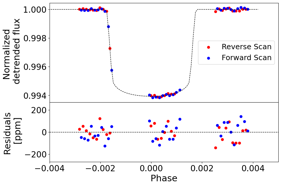
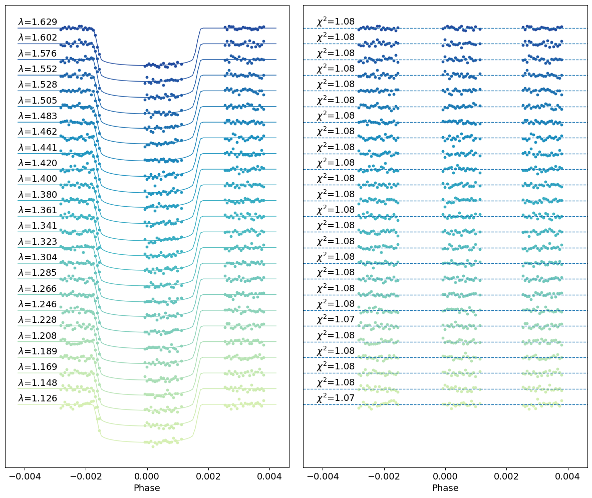
where is the slope of a wavelength-dependent linear systematic trend along each HST visit, is the white light curve and is the best-fit model for the white light curve. The normalisation factor is the averaged out-of-transit flux in each spectral bin centered at . Again, the normalisation factor is changed to for upward scanning directions (forward scanning) and to for downward scanning directions (reverse scanning). The white light curve fit is shown in Figure 1 and the subsequent spectral light-curve fits are shown in Figure 2. A full list of stellar and planet parameters used here for the fitting is given in Table 1. It should be noted that in this work we use the out-of-transit spectrum of the star to model its properties. In principle there could be some chromatic time-dependent systematics in the absolute flux estimations that could affect the retrieval of the stellar properties based on the out-of-transit spectrum of the star. We verified that these systematics, if present, are negligible for our analysis as it is shown it in APPENDIX A. It should also be noted that Iraclis corrections does not correct possible residual wavelength-dependent systematics in the absolute flux.
4 Spectral Analysis
Edwards et al. (2021) suggested the possibility that some features of the spectrum of LHS1140 b could be due to stellar spots contaminations and tried to simulate them. However, the X-ray luminosity value () of LHS 1140 b as reported by Spinelli et al. (2023) put this star at the lower end of the X-ray distribution function ( ) pointing to a quiet old star. Moreover, the analysis of the TESS lightcurves shows no significant signs of activity (Bonney & Kennefick, 2022). LHS 1140 has also a long rotational period of about 131 days (Dittmann et al., 2017; Newton et al., 2018) suggesting a low level of activity (Pizzolato et al., 2003). These observational evidences suggest that LHS 1140 is rather a quiet, inactive star. Therefore, it is rather unlikely that stellar spots might severely affect its stellar spectrum. In the following, we will test the alternative hypothesis that the star has a non-solar chemical composition.
4.1 Stellar Composition
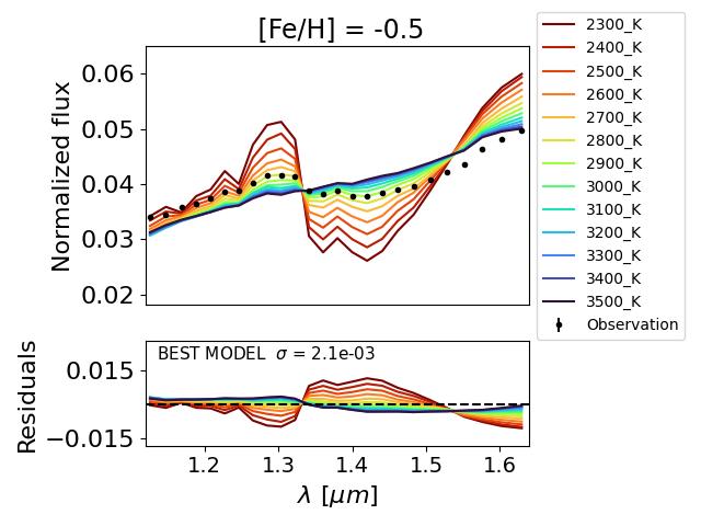
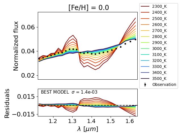
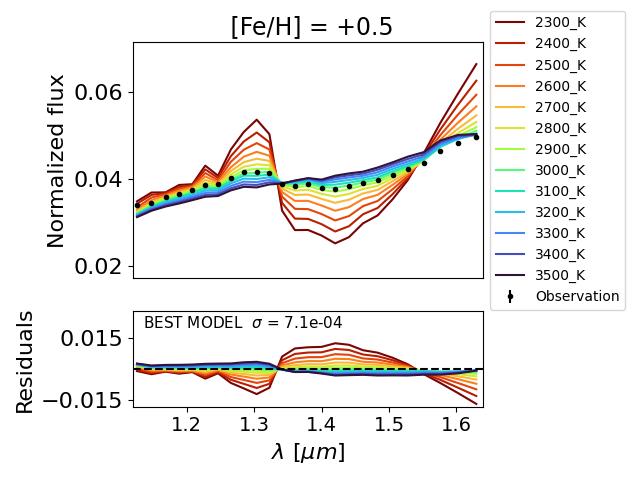
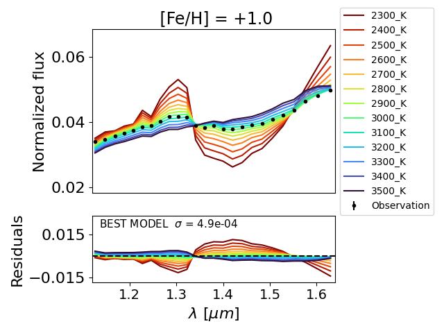
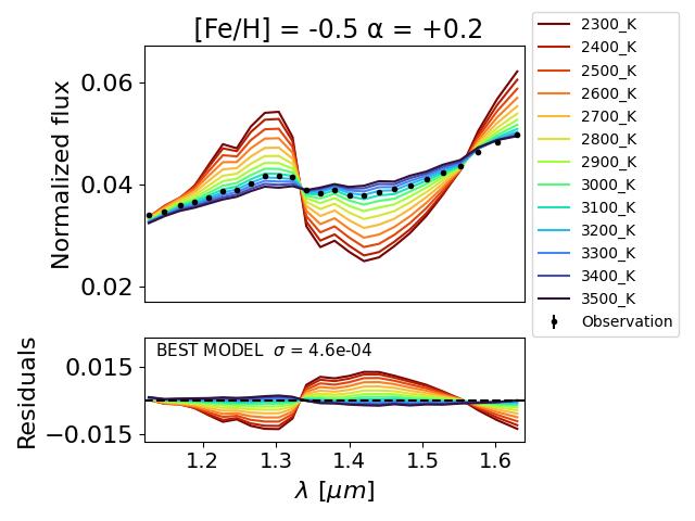
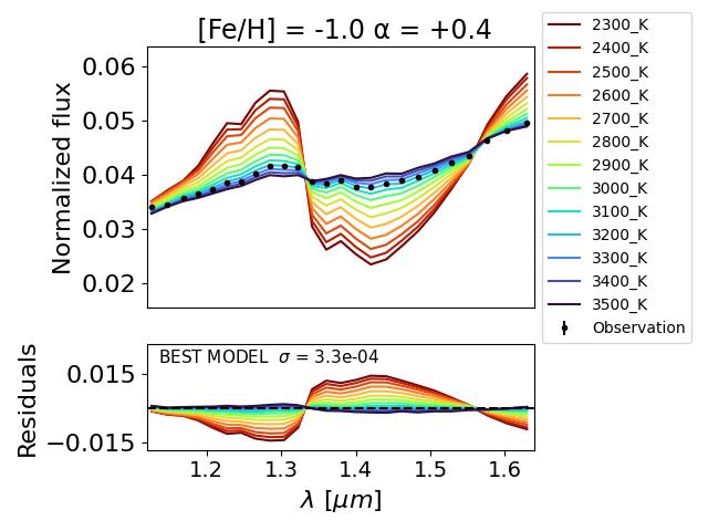
In order to do so, we evaluated various stellar atmospheric models to determine which one could best describe the observed out-of-transit spectrum. We generated a set of stellar spectra obtained from the PHOENIX-2012-2013 database to mimic the stellar photosphere. This involved selecting the models with log(g) =5.0 and with stellar temperature within a wide range (2300-3500 K). We explored several stellar compositions by combining the metallicity [Fe/H] and the value of the star. In particular, we tested the metallicity [Fe/H] within the range [-1.0,1.0] with a 0.5 step. Then, we also evaluate the enrichment for the low metallicities cases: [Fe/H] = -0.5 dex with and [Fe/H] = -1.0 dex with .
The resulting spectra were multiplied for the HST G141 grism sensitivity (calibrated by Kuntschner et al., 2011), accounting for the conversion from flux to electrons units. Two other chromatic components were taken into account: the dispersion of light from the star at the focal plane of the detector due to the grism and the dependence of the PSF (Point Spread Function) on the wavelenght observed. A detailed description of these two effects can be found in Varley et al. (2017). Finally, the spectra are binned by using the same binning used to fit the spectral light curves.
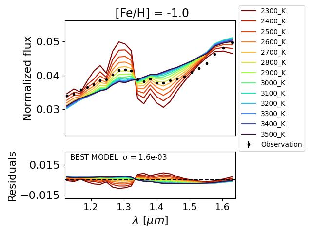
Figures 3 and 4 show a comparison between the data and the various tested models, highlighting how the parameters (temperature, metallicity [Fe/H] and enrichment) impact the shape of the stellar spectrum. Specifically, we observe an increase in the amplitude of the features around at lower temperature, and the rise in flux in the red end of the spectrum at higher metallicity. The residuals between the observed data and the models are shown at the bottom of each plot. Finally in Tab. 2 we show the values of the models at 3100, 3200 and 3300 K, that better fit the observations. Each value is obtained using Eq. 3 where N is the number of spectral bin observed, "" are the observed spectral fluxes and are the theoretical spectral fluxes predicted by the model for the specific stellar composition tested :
| (3) |
| Z | ||||
|---|---|---|---|---|
| -1.0 | 0.0 | |||
| -0.5 | 0.0 | |||
| 0.0 | 0.0 | |||
| +0.5 | 0.0 | |||
| +1.0 | 0.0 | |||
| -0.5 | +0.2 | |||
| -1.0 | 0.4 |
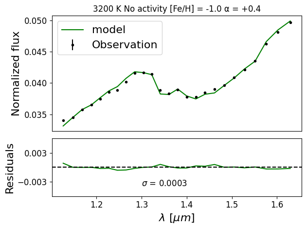
Based on these tests, we identified a model of a quiet star with a combination of temperature, metallicity, and that provides a good representation of the observed out-of-transit spectrum without evidence of chromaticity effects in the residuals, as illustrated in Figure 5. Note that we are comparing the data with a grid of models and not fitting the best temperature. This result, together with other previous evidences of the low level of activity of the star both from XUV observations (see Spinelli et al., 2023) and from TESS almost flat light curves analysis for this target (Bonney & Kennefick, 2022) and the good correspondence between the temperature of this model (3200 K) and that derived by literature (, derived by Ment et al., 2019), strongly suggests to rule out any strong stellar activity contribution in this transit observation. This lack of stellar activity implies that the planetary spectrum does not need a correction for stellar activity contaminations and that its spectral features are only due to the planetary atmosphere.
4.2 Stellar Activity Evaluation
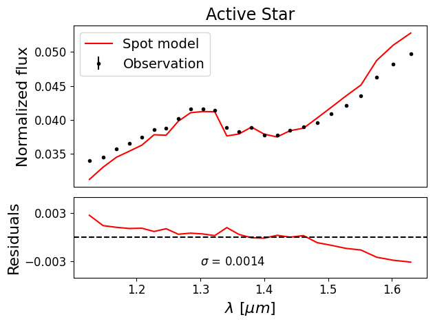
As a further check, we compared the observations with the simulated spectrum of a star with a dominant spot, following the methodology described in Cracchiolo et al. (2021b).
The star is modeled as having one dominant circular spot with radius (normalized to the stellar radius ) on the stellar surface, whose projection onto the stellar disk is an ellipse with eccentricity dependent on the fractional distance between the spot center and the center of the stellar disk. In this case the stellar disk is divided into N = 10 000 annuli, each with radius and width , and characterized by an emission given by a linear combination between the intensity emitted from the spot and the intensity emitted from photosphere.
The out-of-transit flux will be obtained by summing up the intensities from all the annuli:
| (4) |
where is the fraction of the annulus covered by the spot. and are the intensity profiles emitted from the photosphere and from the spot, respectively, for each annulus. Each intensity profile is obtained with a 4-coefficients limb darkening law (Claret et al., 2012):
| (5) |
with and the four LDCs. Here, we neglected the dependence of the limb darkening effect on the temperature and we assumed the same LDCs (the same from Edwards et al., 2021) for the spots and the photosphere.
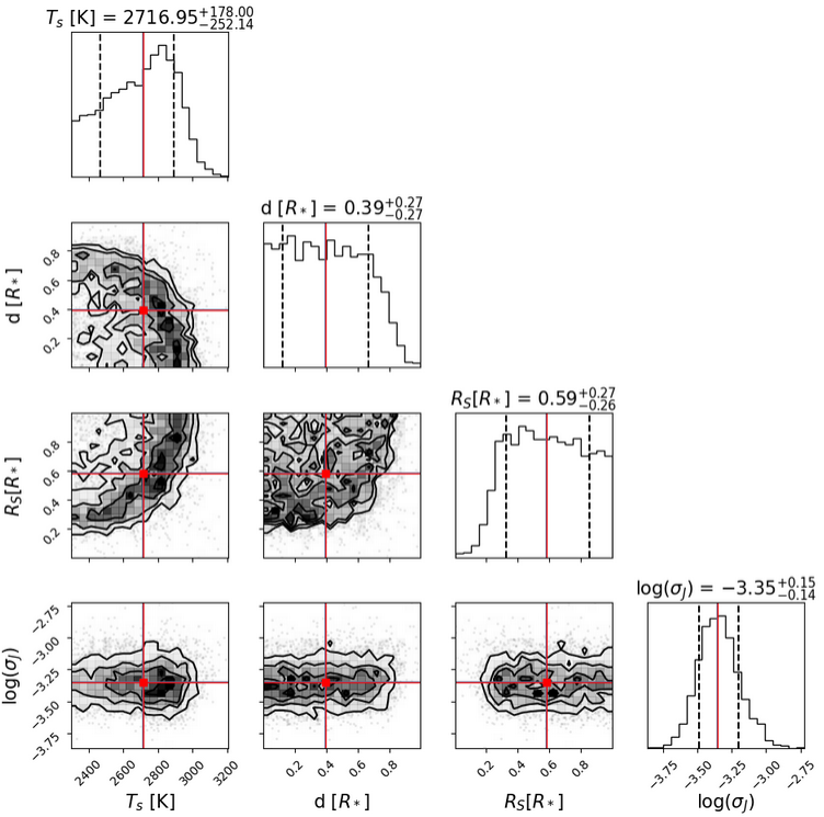
This model identifies the spot with 3 parameters: d, and . Using as fitting algorithm the MCMC code emcee with the same methodology of Cracchiolo et al. (2021b) we obtained as a result the fit showed in Figure 5.
Comparing the results of the model corresponding to a different composition of the star and the results of the model involving spot presence (Figure 5) it is clear that the
second one has a standard deviation much higher than the first one and a clear chromaticity of the residuals. Furthermore, the results of the fit accounting for the stellar activity suggest the presence of a big spot, with , results not compatible with the results of Spinelli et al. (2023) which found a low level of activity for LHS 1140.
As a consequence we are quite confident that the spectral modulation studied by Edwards et al. (2021) is due to the planetary atmosphere without relevant stellar activity contamination. Our results also suggests that stellar composition must be considered in analysis of exoplanetary transmission spectra.
5 Stellar Population Membership
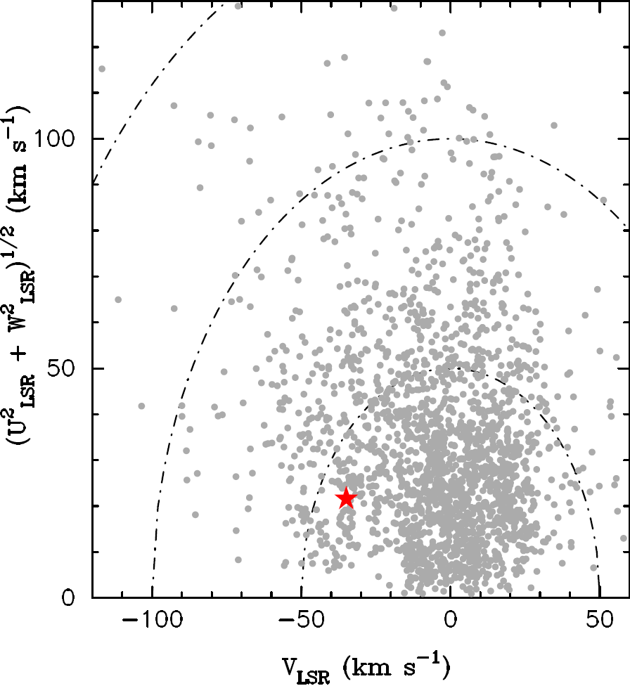
Low metallicity values and -element enrichment are typical of old stars of the thick disk (compatible with the estimated age of this star billion years, Spinelli et al., 2019). We, therefore, analysed the kinematics of the target to determine its kinematics age. Galactic-spatial velocity components (, , ) were computed using Gaia DR3 (Gaia Collaboration et al., 2023) proper motions, parallax and radial velocities by using the methodology described in Maldonado et al. (2010, 2020).
The derived values are , and , while the corresponding Toomre diagram is shown in Figure 7. To classify the star as belonging to the thin/thick disc population we made use of the procedure described by Bensby et al. (2003, 2005). We found that LHS1140 shows a kinematics compatible with an old thin disk star, populating the most external thin disk region of the Toomre diagram (Figure 7). However, the kinematics criterion is a statistical one and alone is not enough to classify an individual star as a member of the thick or thin disk population.
In order to further clarify the chemical composition of LHS 1140, we analysed the available HARPS high-resolution optical spectra of this star. We use the methodology developed in Maldonado et al. (2020) which is based on the use of principal component analysis and sparse Bayesian methods and is calibrated using M dwarfs in binary systems around an FGK primary. We derived a metallicity value of [Fe/H] = -0.38 dex, thus, confirming that LHS 1140 is a metal poor star. Moreover, we find that elements show higher abundances ([Mg/H] = 0.01 dex, [Si/H] = -0.15 dex, [Ca/H] = -0.10 dex).
We should caution to use quantitative results from Maldonado et al. (2020) since it might not be optimal for metal poor stars, as the number of "training" stars in this region of metallicities is rather low.
However also this analysis points toward a poor metal star with enhanced elements, that cannot be properly described by assuming solar-like atmospheric composition models.
| Parameter | Prior Bounds | Scale |
|---|---|---|
| -12, 0 | ||
| 50, 500 | linear | |
| -4, 6 | ||
| 0.123, 0.185 | linear | |
| 0.172 | fixed | |
| 0.2 | fixed |
6 Atmospheric Retrieval
Given our analysis of the chemical composition of LHS 1140 and the consequent attribution of the features of the in-transit spectrum to the planet, we reviewed the work of Edwards et al. (2021) analyzing the planetary spectrum by using the Taurex retrieval framework (Al-Refaie et al., 2021) with the same priors of Edwards et al. (2021) (shown in Tab. 3) and an expanded grid of atmospheric parameters with different combinations of , , and clouds as in Table 4.
Our aim was to confirm the results of Edwards et al. (2021) using the updated values for the planetary mass and radius from Cadieux et al. (2023), because the mass in particular can have a relevant impact in atmospheric retrievals (Di Maio et al., 2023).
We wanted also to include the flat case of an atmosphere without any relevant molecular contribution in the planetary spectrum for reference.
In order to efficiently explore the parameter space, TauREx uses the MultiNest optimizer (Feroz et al., 2009; Buchner et al., 2014) and we chose to use 3000 live points to achieve a higher precision for our fits.
To efficiently explore the parameter space, we used TauREx with the MultiNest optimizer, employing 3000 live points to enhance fitting precision. In our retrieval procedure we used the molecular cross sections of and taken from Polyansky et al. (2018) and Yurchenko et al. (2017) respectively. Finally we took into account collision-induced-absorption (CIA) due to
(Abel et al., 2011; Fletcher et al., 2018) and to and also Rayleigh scattering for alle the molecules in the atmosphere.
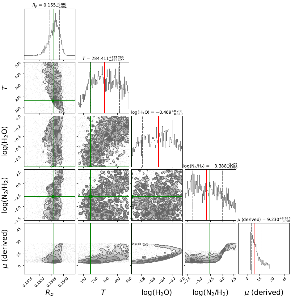
Following the criterion illustrated in Kass & Raftery (1995), bayesian evidence does not allow us to identify any specific atmospheric composition, probably because of the wavelength range and low resolution of our data that do not allow us to distinguish the bands of the specific molecules. However, the bayesian evidence suggests that the hypothesis of a flat atmosphere can be rejected. Furthermore it led to a slightly higher probability for comprehensive scenarios (Table 4) with respect to rich atmosphere. The corner plot corresponding to the best fit is shown in Figure 8.
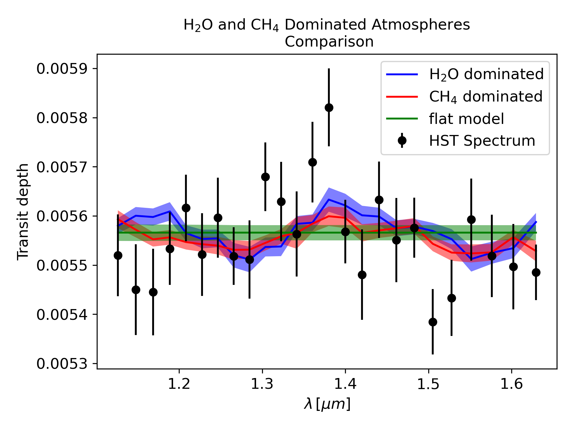
Figure 9 instead shows the comparison between the observed HST data and the two most extreme scenarios that we simulated: H2O dominated and CH4-dominated atmosphere, without cloud contributions. It is clear from the figure that, despite some small differences, both curves are similar and hard to distinguish.
7 Conclusions
LHS 1140 b is a planet close to the HZ of its host star. Previous studies (e.g. Edwards et al., 2021) analyzed its atmosphere suggesting the presence of water, but could not rule out the possibility that the modulation of the in-transit spectrum could be due to stellar activity contamination.
In this work, we found that the out-of-transit spectra of LHS 1140 during HST observations can be explained by a quiet, inactive star, with low [Fe/H] and high abundances, so the difference between the in- and -out transit spectra can be entirely attributed to the LHS 1140 b planet atmosphere. Therefore, we are confident that the derived planetary spectrum is not contaminated by a significant stellar contribution and that any spectral feature presented does indeed reflects the planetary atmosphere of LHS 1140 b.
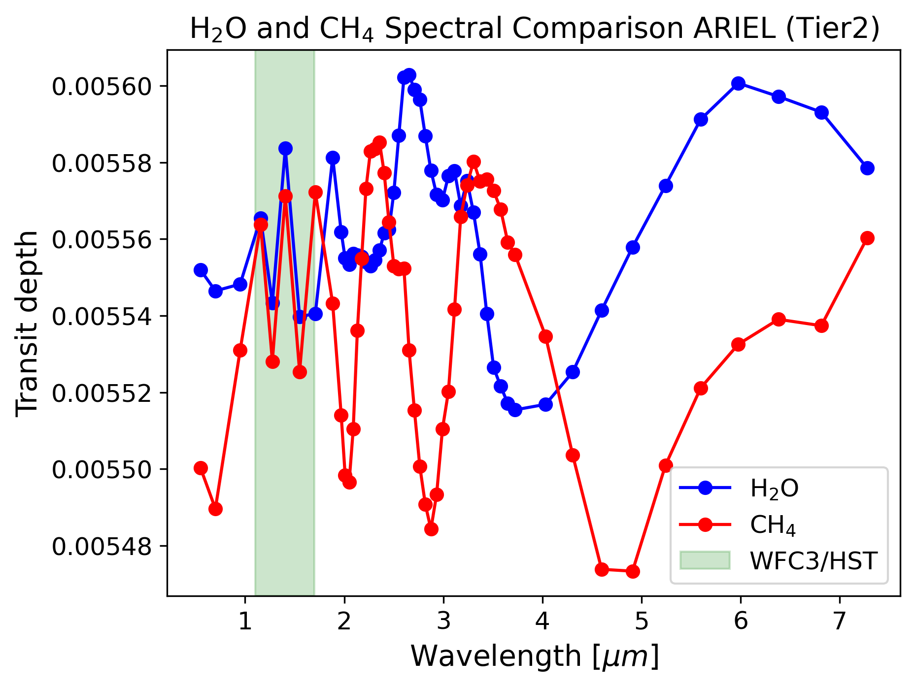
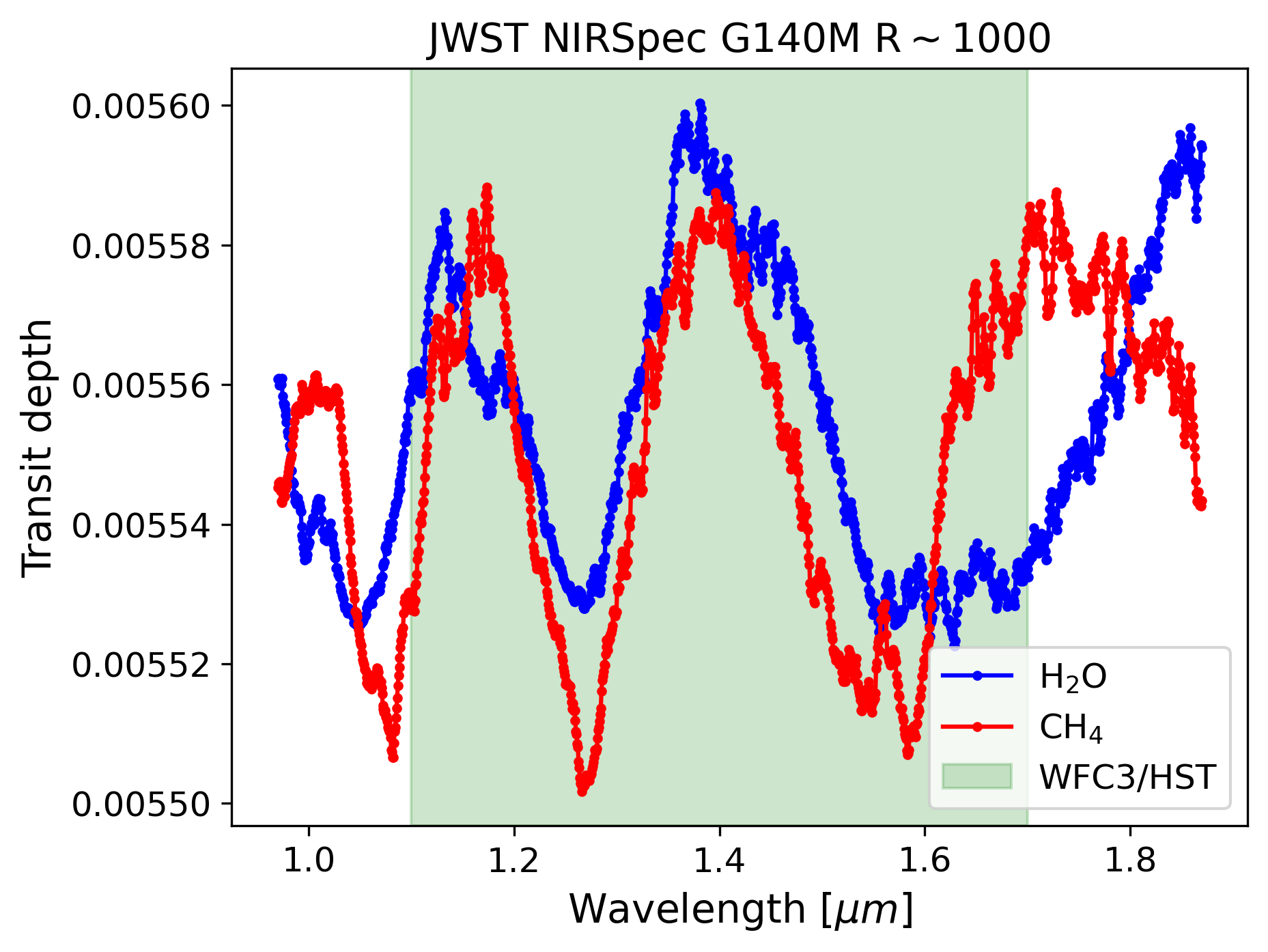
A proper evaluation of the atmospheric composition of LHS 1140 b will therefore require additional observations, as example with JWST or the upcoming Ariel mission, with higher spectral resolution or broader band coverage. In particular, we simulated the atmospheric signal of LHS 1140 b during a transit as observed with ARIEL tier 2, obtained through ARIELRAD (Mugnai et al., 2019) and we did the same also for JWST Nirspec (Jakobsen et al., 2022) with G140M grism, using PANDEXO (Batalha et al., 2017) to simulate the expected observed flux for this target. Figure 10 shows the results of this simulations, that is, the comparison between the simulated atmosphere of LHS 1140 b with the same scenarios analyzed in Figure 9. It can be seen that the difference between both cases is quite clear, and therefore detectable with ARIEL or JWST observations, mainly thanks to the long wavelength coverage, thus, allowing us to confirm or rule out the presence of water on the planet and to retrieve its abundance. The challenges in properly modeling the atmosphere of LHS 1140 b using HST WFC3 observations may arise from their low resolution and narrow spectral range together with a low signal to noise.
We finally stress the importance of an accurate modelling of the host stellar spectra, not limited to stellar activity but including also its chemical composition, when dealing with suspect features in the retrieved in-transit spectra.
| MODEL | log | T (K) | log() | log() | log() | log | |
| no clouds | 195.0 | - | - | ||||
| -clouds | 194.4 | - | |||||
| no clouds | 193.9 | - | |||||
| -clouds | 193.6 | ||||||
| -clouds | 192.7 | - | |||||
| no clouds | 192.6 | - | - | ||||
| no clouds | 191.7 | - | - | - | |||
| no clouds | 191.4 | - | - | - | |||
| -clouds | 191.1 | - | - | ||||
| -clouds | 191.0 | - | - | ||||
| -clouds | 191.0 | - | - | ||||
| -clouds | 191.0 | - | - | ||||
| flat model | 190.4 | - | - | - | - | ||
| no clouds | 189.9 | - | - | - | |||
| no clouds | 189.5 | - | - | - |
Acknowledgements
The authors acknowledge the support of the ASI-INAF agreement n. 2021-5-HH.0 and thank Angelos Tsiaras for his invaluable contribution in the processing and the reduction of HST WFC3 data, and Billy Edward for his helpful advices.
J. M. acknowledges support from the Italian Ministero dell’Università e della Ricerca and from the European Union - Next Generation EU through project PRIN MUR 2022PM4JLH “Know your little neighbours: characterizing low-mass stars and planets in the Solar neighbourhood”.
Based on data products from observations made with ESO Telescopes at the La Silla Paranal Observatory under programms ID 191.C-0873(A), 198.C-0838(A), 100.C-0884(A), 60.A-9709(G).
Part of the research activities described in this paper were carried out with contribution of the Next Generation EU funds within the National Recovery and Resilience Plan (PNRR), Mission 4 - Education and Research, Component 2 - From Research to Business (M4C2), Investment Line 3.1 - Strengthening and creation of Research Infrastructures, Project IR0000034 – “STILES - Strengthening the Italian Leadership in ELT and SKA”.
Data Availability
The analysis shown in this paper is derived from publicly available data and codes: https://archive.stsci.edu/hst/ (MAST portal), https://github.com/ucl-exoplanets/Iraclis (Iraclis, Tsiaras et al., 2018), https://phoenix.ens-lyon.fr/Grids/ (Phoenix, Claret et al., 2012)
https://github.com/ucl-exoplanets/TauREx3_public (TauReX, Al-Refaie et al., 2021), https://github.com/ucl-exoplanets/pylightcurve (pylightcurve, Tsiaras et al., 2016), https://emcee.readthedocs.io/en/stable/ (emcee, Foreman-Mackey et al., 2013a).
The specific result can be shared on reasonable request to the corresponding author.
References
- Abel et al. (2011) Abel M., Frommhold L., Li X., Hunt K. L. C., 2011, Journal of Physical Chemistry A, 115, 6805
- Agol et al. (2010) Agol E., Cowan N. B., Knutson H. A., Deming D., Steffen J. H., Henry G. W., Charbonneau D., 2010, ApJ, 721, 1861
- Al-Refaie et al. (2021) Al-Refaie A. F., Changeat Q., Waldmann I. P., Tinetti G., 2021, ApJ, 917, 37
- Ballerini et al. (2012) Ballerini P., Micela G., Lanza A. F., Pagano I., 2012, A&A, 539, A140
- Batalha et al. (2017) Batalha N. E., et al., 2017, PASP, 129, 064501
- Bensby et al. (2003) Bensby T., Feltzing S., Lundström I., 2003, A&A, 410, 527
- Bensby et al. (2005) Bensby T., Feltzing S., Lundström I., Ilyin I., 2005, A&A, 433, 185
- Berdyugina (2005) Berdyugina S. V., 2005, Living Reviews in Solar Physics, 2, 8
- Berta et al. (2011) Berta Z. K., Charbonneau D., Bean J., Irwin J., Burke C. J., Désert J.-M., Nutzman P., Falco E. E., 2011, ApJ, 736, 12
- Berta et al. (2012) Berta Z. K., Irwin J., Charbonneau D., Burke C. J., Falco E. E., 2012, AJ, 144, 145
- Bonney & Kennefick (2022) Bonney P., Kennefick J., 2022, in American Astronomical Society Meeting Abstracts. p. 309.03
- Buchner et al. (2014) Buchner J., et al., 2014, A&A, 564, A125
- Cadieux et al. (2023) Cadieux C., et al., 2023, arXiv e-prints, p. arXiv:2310.15490
- Claret et al. (2012) Claret A., Hauschildt P. H., Witte S., 2012, A&A, 546, A14
- Cracchiolo et al. (2021a) Cracchiolo G., Micela G., Peres G., 2021a, MNRAS, 501, 1733
- Cracchiolo et al. (2021b) Cracchiolo G., Micela G., Morello G., Peres G., 2021b, MNRAS, 507, 6118
- Czesla et al. (2009) Czesla S., Huber K. F., Wolter U., Schröter S., Schmitt J. H. M. M., 2009, A&A, 505, 1277
- Deming et al. (2013) Deming D., et al., 2013, ApJ, 774, 95
- Désert et al. (2011) Désert J. M., et al., 2011, A&A, 526, A12
- Di Maio et al. (2023) Di Maio C., Changeat Q., Benatti S., Micela G., 2023, A&A, 669, A150
- Diamond-Lowe et al. (2020) Diamond-Lowe H., Berta-Thompson Z., Charbonneau D., Dittmann J., Kempton E. M. R., 2020, AJ, 160, 27
- Dittmann et al. (2017) Dittmann J. A., et al., 2017, Nature, 544, 333
- Edwards et al. (2021) Edwards B., et al., 2021, AJ, 161, 44
- Feroz et al. (2009) Feroz F., Hobson M. P., Bridges M., 2009, MNRAS, 398, 1601
- Fletcher et al. (2018) Fletcher L. N., Gustafsson M., Orton G. S., 2018, ApJS, 235, 24
- Foreman-Mackey et al. (2013a) Foreman-Mackey D., et al., 2013a, emcee: The MCMC Hammer, Astrophysics Source Code Library, record ascl:1303.002 (ascl:1303.002)
- Foreman-Mackey et al. (2013b) Foreman-Mackey D., Hogg D. W., Lang D., Goodman J., 2013b, PASP, 125, 306
- Gaia Collaboration et al. (2023) Gaia Collaboration et al., 2023, A&A, 674, A1
- Gardner et al. (2006) Gardner J. P., et al., 2006, Space Sci. Rev., 123, 485
- Gomes & Ferraz-Mello (2020) Gomes G. O., Ferraz-Mello S., 2020, MNRAS, 494, 5082
- Greene et al. (2016) Greene T. P., Line M. R., Montero C., Fortney J. J., Lustig-Yaeger J., Luther K., 2016, ApJ, 817, 17
- Jakobsen et al. (2022) Jakobsen P., et al., 2022, A&A, 661, A80
- Kane (2018) Kane S. R., 2018, ApJ, 861, L21
- Kass & Raftery (1995) Kass R. E., Raftery A. E., 1995, Journal of the American Statistical Association, 90, 773
- Kreidberg et al. (2014) Kreidberg L., et al., 2014, Nature, 505, 69
- Kuntschner et al. (2011) Kuntschner H., Kümmel M., Walsh J. R., Bushouse H., 2011, Revised Flux Calibration of the WFC3 G102 and G141 grisms, ST-ECF Instrument Science Report WFC3-2011-05, 13 pages
- Maldonado et al. (2010) Maldonado J., Martínez-Arnáiz R. M., Eiroa C., Montes D., Montesinos B., 2010, A&A, 521, A12
- Maldonado et al. (2020) Maldonado J., et al., 2020, A&A, 644, A68
- Mayor et al. (2003) Mayor M., et al., 2003, The Messenger, 114, 20
- McCullough & MacKenty (2012) McCullough P., MacKenty J., 2012, Considerations for using Spatial Scans with WFC3, Instrument Science Report WFC3 2012-08, 17 pages
- Ment et al. (2019) Ment K., et al., 2019, AJ, 157, 32
- Micela (2015) Micela G., 2015, Experimental Astronomy, 40, 723
- Mugnai et al. (2019) Mugnai L., Edwards B., Papageorgiou A., Pascale E., Sarkar S., 2019, 2019, EPSC
- Newton et al. (2018) Newton E. R., Mondrik N., Irwin J., Winters J. G., Charbonneau D., 2018, AJ, 156, 217
- Pizzolato et al. (2003) Pizzolato N., Maggio A., Micela G., Sciortino S., Ventura P., 2003, A&A, 397, 147
- Polyansky et al. (2018) Polyansky O. L., Kyuberis A. A., Zobov N. F., Tennyson J., Yurchenko S. N., Lodi L., 2018, MNRAS, 480, 2597
- Pont et al. (2008) Pont F., Knutson H., Gilliland R. L., Moutou C., Charbonneau D., 2008, MNRAS, 385, 109
- Salz et al. (2018) Salz M., et al., 2018, A&A, 620, A97
- Scandariato & Micela (2015) Scandariato G., Micela G., 2015, Experimental Astronomy, 40, 711
- Sing et al. (2009) Sing D. K., Désert J. M., Lecavelier Des Etangs A., Ballester G. E., Vidal-Madjar A., Parmentier V., Hebrard G., Henry G. W., 2009, A&A, 505, 891
- Sing et al. (2011a) Sing D. K., et al., 2011a, MNRAS, 416, 1443
- Sing et al. (2011b) Sing D. K., et al., 2011b, A&A, 527, A73
- Solanki (2003) Solanki S. K., 2003, A&ARv, 11, 153
- Spinelli et al. (2019) Spinelli R., Borsa F., Ghirlanda G., Ghisellini G., Campana S., Haardt F., Poretti E., 2019, A&A, 627, A144
- Spinelli et al. (2023) Spinelli R., Gallo E., Haardt F., Caldiroli A., Biassoni F., Borsa F., Rauscher E., 2023, AJ, 165, 200
- Thompson et al. (2023) Thompson A., et al., 2023, arXiv e-prints, p. arXiv:2302.04574
- Tinetti et al. (2018) Tinetti G., et al., 2018, Experimental Astronomy, 46, 135
- Tsiaras et al. (2016) Tsiaras A., Waldmann I. P., Rocchetto M., Varley R., Morello G., Damiano M., Tinetti G., 2016, ApJ, 832, 202
- Tsiaras et al. (2018) Tsiaras A., et al., 2018, AJ, 155, 156
- Varley et al. (2017) Varley R., Tsiaras A., Karpouzas K., 2017, ApJS, 231, 13
- Werner et al. (2004) Werner M. W., et al., 2004, ApJS, 154, 1
- Wunderlich et al. (2019) Wunderlich F., et al., 2019, A&A, 624, A49
- Yurchenko et al. (2017) Yurchenko S. N., Amundsen D. S., Tennyson J., Waldmann I. P., 2017, A&A, 605, A95
- Zacharias et al. (2013) Zacharias N., Finch C. T., Girard T. M., Henden A., Bartlett J. L., Monet D. G., Zacharias M. I., 2013, AJ, 145, 44
Appendix A Pre and Post Transit Comparison
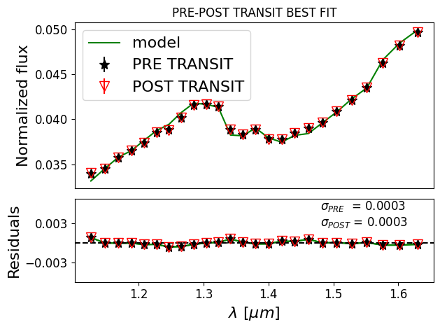
As discussed in section 3, processed data could be affected by time-dependent chromatic effects. For this reason we analyzed separately the pre-transit and post transit data to look for any relevant difference, possible clue of time-dependent systematics in our data. In Fig. 11 we show the resulting out-of-transit stellar spectra before and after transit. These two spectra clearly match each other and their differences are lower than their associated error and much lower than the differences between these spectra and their common best model. As a further check, we performed the analysis using only pre or post transit spectra to verify the self-consistency of our results about the stellar composition of the star. The results obtained from those analyses (see Table 5) are consistent with the results reported in Table 2 confirming the self-consistency of our approach and the temperature and metallicity found in section 4.1.
| Z | ||||
|---|---|---|---|---|
| pre/post | pre/post | pre/post | ||
| -1.0 | 0.0 | |||
| -0.5 | 0.0 | |||
| 0.0 | 0.0 | |||
| +0.5 | 0.0 | |||
| +1.0 | 0.0 | |||
| -0.5 | +0.2 | |||
| -1.0 | 0.4 |