LayerNorm: A key component in parameter-efficient fine-tuning

Abstract

Fine-tuning a pre-trained model, such as Bidirectional Encoder Representations from Transformers (BERT), has been proven to be an effective method for solving many natural language processing (NLP) tasks. However, due to the large number of parameters in many state-of-the-art NLP models, including BERT, the process of fine-tuning is computationally expensive. One attractive solution to this issue is parameter-efficient fine-tuning, which involves modifying only a minimal segment of the model while keeping the remainder unchanged. Yet, it remains unclear which segment of the BERT model is crucial for fine-tuning. In this paper, we first analyze different components in the BERT model to pinpoint which one undergoes the most significant changes after fine-tuning. We find that output LayerNorm changes more than any other components when fine-tuned for different General Language Understanding Evaluation (GLUE) tasks. Then we show that only fine-tuning the LayerNorm can reach comparable, or in some cases better, performance to full fine-tuning and other parameter-efficient fine-tuning methods. Moreover, we use Fisher information to determine the most critical subset of LayerNorm and demonstrate that many NLP tasks in the GLUE benchmark can be solved by fine-tuning only a small portion of LayerNorm with negligible performance degradation.

Keywords Parameter-Efficient Fine-Tuning  $\cdot$ LayerNorm  $\cdot$ Large Language Model  $\cdot$ Fisher Information

1 Introduction

Transformer-based (Vaswani et al., 2017) Large Language Models (LLMs), such as Bidirectional Encoder Representations from Transformers (BERT) (Devlin et al., 2018), Robustly optimized BERT approach (RoBERTa) (Liu et al., 2019), and XLNet (Yang et al., 2019b), yield splendid performance for many natural language processing (NLP) tasks, outperforming traditional word embedding models, such as Word2Vec (Mikolov et al., 2013) and GloVe (Pennington et al., 2014). Such models are first pre-trained on a huge corpus of unlabelled text, and then are fine-tuned for a specific downstream task.

Despite their excellent performance, these models are computationally expensive for fine-tuning (Zhao et al., 2019; Guo et al., 2020; Zaken et al., 2021; Radiya-Dixit & Wang, 2020; Gordon et al., 2020) due to their large number of parameters. This cost grows with increasing the number of tasks learned (Radiya-Dixit & Wang, 2020). Moreover, such models with the large number of parameters in conjunction with limited labeled data for the downstream task are prone to overfitting and hence poor generalization performance for out-of-distribution data (Aghajanyan et al., 2021; mahabadi et al., 2021; Xu et al., 2021). One popular approach to this issue is to only train a small portion of the model, rather than performing a full fine-tuning. For instance, Radiya-Dixit & Wang (2020) only trained 60 % of BERT parameters. Recently, Zaken et al. (2021) only trained bias parameters of BERT, which reached results that are comparable with full fine-tuning. We hypothesize, however, that the bias may not necessarily be the optimal component of BERT for parameter-efficient fine-tuning, and similar/better performance could be obtained by training a smaller number of parameters if the optimal component is chosen.

In this paper, we use BERT as an example to test our hypothesis. First, we examine how different components of BERT change during the full fine-tuning and discover that LayerNorm is a key component in fine-tuning. Second, we show that LayerNorm possesses the maximum Fisher information among all the components of BERT. Third, we demonstrate that just training LayerNorm can reach the similar performance as only training bias, yet with one-fifth number of parameters. Finally, we show that a comparable performance can be obtained even with only a portion of the LayerNorm, where such a portion can be obtained from the information available in the down-stream task at hand, or other down-stream tasks.

The rest of this paper is organized as follows. In Section 2, we demonstrate that LayerNorm is a key component in fine-tuning BERT. In Section 3, we present our method by only training LayerNorm and the results. Section 4 is dedicated to the discussions. Related works are reviewed in Section 5. Finally, the conclusions and the future works are provided in Section 6. A detailed description of LayerNorm is provided in Appendix A.

2 A key component of BERT

BERT consists of multiple layers, and in each layer there are different components, such as self-attention, feed-forward network, and LayerNorm. Our goal in this section is to pinpoint the most important component for fine-tuning. Radiya-Dixit & Wang (2020) demonstrated that in the BERT model, $L_{1}$ distance (See Appendix B for definitions) between the pre-trained model and the fine-tuned model is significantly lower than the $L_{1}$ distance between two independent random initialed models, or the distance between parameters before and after pre-training. This indicates that during the process of fine-tuning, the model parameters only undergo small changes. Additionally, good fine-tuned models exist that can have a small $L_{0}$ distance from the pre-trained model (Zaken et al., 2021; Radiya-Dixit & Wang, 2020). A small $L_{0}$ means that many parameters do not need to change. As such, we can achieve a good fine-tuning performance without training all the components. Therefore, the question is which components ought to be fine-tuned and which components do not need to change.

2.1 Data

We used the General Language Understanding Evaluation (GLUE) (Wang et al., 2019) dataset, which has been used in different studies (Houlsby et al., 2019b; Guo et al., 2020; Zaken et al., 2021; Xu et al., 2021) as the standard benchmark in this field. GLUE dataset consists of different tasks, namely, the Corpus of Linguistic Acceptability (CoLA) (Warstadt et al., 2019), the Stanford Sentiment Treebank (SST2) (Socher et al., 2013), the Microsoft Research Paraphrase Corpus (MRPC) (Dolan & Brockett, 2005), the Semantic Textual Similarity Benchmark (STS-B) (Cer et al., 2017), the Quora Question Pairs (QQP) (Iyer et al., 2017), the Multi-Genre Natural Language Inference Corpus (MNLI) (Williams et al., 2018), the Stanford Question Answering Dataset (QNLI) (Rajpurkar et al., 2016), and the Recognizing Textual Entailment (RTE) (Dagan et al., 2006; Bar-Haim et al., 2006; Giampiccolo et al., 2007; Bentivogli et al., 2009). We excluded the Winograd Schema Challenge (WNLI) (Levesque et al., 2012) since the results for WNLI are unreliable (Prasanna et al., 2020). Many other studies have also excluded this task (Devlin et al., 2019; Zaken et al., 2021; Xu et al., 2021). Table 4 in Appendix C shows the metric employed for the evaluation of each task.

2.2 Pipeline

Low training cost can be achieved by only training a small subset of the model, which is equivalent to having a small $L_{0}$ distance between the pre-trained and the fine-tuned model. Our goal is to find out which components in BERT must be frozen and which components must be trained in order to have a good performance and a low training cost. To achieve the goal, we directly addressed the following tangigle question: During the process of full fine-tuning, which components of the model undergo significant changes? To proceed, we fine-tuned BERT-large-cased for different tasks in GLUE (Wang et al., 2019). After fine-tuning, for each component, we compared the original value and the fine-tuned value of the parameters. For an array of all parameters in a component before fine-tuning (${C_{pre}}_{i}$) and after fine-tuning (${C_{fine}}_{i}$), where $i$ represents the index of different values in the component, and the size of the component is $n$, the change after fine-tuning, $D$, is defined as:

$$D=\frac{1}{n}\sum_{i=1}^{n}|{C_{fine}}_{i}-{C_{pre}}_{i}|$$ (1)

which is equal to the $L_{1}$ distance normalized by the length of the vector, to compensate for different sizes in different components.

For all the components at different layers, we calculated $D$ and plotted the heat map for different GLUE tasks. These heat maps are presented in Figure 1. For most GLUE tasks, we observed that the most significant change happens in the output LayerNorm, which we simply call LayerNorm.

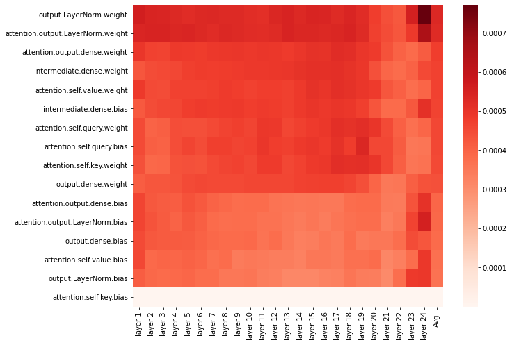
(a) RTE

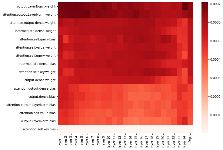
(b) MRPC

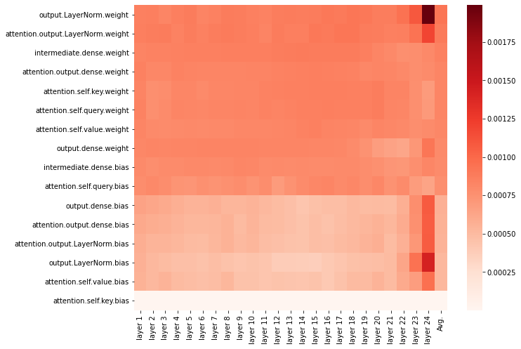
(c) STSB

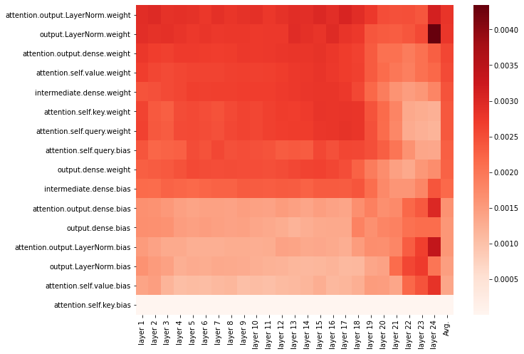
(d) SST2

Figure 1: Heat map of change in each component after fine-tuning for different GLUE tasks.

2.3 Effect of disabling LayerNorm

Various studies have shown that Transformer-based models are, in general, remarkably robust to pruning (Michel et al., 2019; Gordon et al., 2020; Prasanna et al., 2020; Chen et al., 2020), which means that removing parts of the model does not have a severe effect on its performance. Contrary to this, it has been shown by Kovaleva et al. (2021) that the performance of models from the BERT family degrades significantly if one component, LayerNorm, is disabled in the model. As an example, removing only 24 parameters in LayerNorm of RoBERTa (Liu et al., 2019) increases the loss of validation of WikiText (Merity et al., 2016) by nearly a factor of 4.

2.4 Search for the most important component using Fisher information

Similar to Xu et al. (2021), we used the Fisher information to choose which component to fine-tune and which to freeze. Fisher information is essentially an estimation of how much information a variable carries about a parameter of a distribution (Tu et al., 2016) and has proven to be a good metric to measure how important a certain parameter in a neural network is (Kirkpatrick et al., 2016; Xu et al., 2021). In a dataset with $N$ samples, where $\mathbf{X_{j}}$ represents the $j$-th input sample and $y_{j}$ represents the $j$-th output, and $\omega$ represents parameters, the Fisher information for the $i$-th parameter can be represented as:

$$F(\omega^{(i)})=\frac{1}{N}\sum_{j=1}^{N}{({\frac{\partial log(p(y_{j}|\mathbf{x_{j}};\omega^{(i)}))}{\partial\omega^{(i)}}})^{2}}$$ (2)

In each task, before running the fine-tuning, we showed the data to the model and calculated the gradient of all the parameters in all the components. Then we calculated the Fisher information of each parameter and obtained the average Fisher information of each component in each task. For each task, we normalized the Fisher information of each component by dividing it by the sum of all information in that task. The rationale for the normalization was to avoid the information of a task, where the total information is small, being overshadowed by a task where the total information is big, and ensure that all of the tasks equally contribute to the final result. After calculating the total information, we sorted the components in descending order, based on their total information in all tasks. The results are presented in Table 1. Again, we can see that “output.LayerNorm”, which we call LayerNorm, has the maximum Fisher information, and “attention.output.LayerNorm”, which we will call attention LayerNorm, comes the second.

Table 1: BERT components sorted by the sum of normalized Fisher information in GLUE tasks.

Rank	Component
1	output.LayerNorm
2	attention.output.LayerNorm
3	attention.output.dense
4	attention.self.value
5	output.dense
6	attention.self.query
7	intermediate.dense
8	attention.self.key

3 Proposed method: Only training LayerNorm

Based on the previous analysis and the observation of Kovaleva et al. (2021), we hypothesized that freezing most of the BERT and only training LayerNorm would result in performance comparable to full fine-tuning. We provided several experiments to test this hypothesis.

3.1 Fine-tuning results

In this section, we reported the details of fine-tuning BERT-large-cased (Devlin et al., 2018). For each GLUE task, we tested the fine-tuning of the full model, bias only (BitFit) (Zaken et al., 2021), LayerNorm only (our proposed method), and fine-tuning the same number of parameters as LayerNorm that were randomly selected. The random parameter experiment was performed as a control to show that the good performance of LayerNorm can not be obtained by any random choice of parameters. In each experiment, we tried 4 different learning rates on the validation set and selected the best. For full fine-tuning, we used the learning rates of $1*10^{-5}$, $2*10^{-5}$, $3*10^{-5}$, and $5*10^{-5}$, and for parameter-efficient fine-turnings (LayerNorm, BitFit, and random) we used $1*10^{-4}$, $4*10^{-4}$, $7*10^{-4}$, and $1*10^{-3}$. In all cases, we tried 20 epochs to select the best number of epochs. The development set results were obtained on our servers and are presented in Table 2. Since for some GLUE tasks the true labels of the test data are held privately, we obtained test set results by submitting our test results to the GLUE benchmark website (GLU, 2021). Test results are shown in Table 3. The full model has 333,581,314 parameters, the BitFit method has 274,434 parameters and LayerNorm has 51,202 parameters, which is less than one-fifth of the number of parameters in the BitFit method.

Table 2: Development set results of fine-tuning BERT large cased for different GLUE tasks, using different methods.

	% of full	QNLI	SST2	MNLI-m	MNLI-mm	CoLA	MRPC	STSB	RTE	QQP
Full	100%	0.9143	0.9335	0.8559	0.8567	0.6554	0.9239	0.9091	0.7653	0.8769
BitFit	0.082%	0.9145	0.9278	0.8399	0.8457	0.6364	0.9183	0.9043	0.7473	0.8476
LayerNorm	0.015%	0.9072	0.9312	0.8285	0.8348	0.6412	0.9130	0.9039	0.7401	0.8361
Random	0.015%	0.8975	0.9220	0.8113	0.8105	0.5851	0.8493	0.8822	0.6065	0.8391

Table 3: Test set results of fine-tuning BERT large cased for different GLUE tasks, using different methods.

	% of full	QNLI	SST2	MNLI-m	MNLI-mm	COLA	MRPC	STSB	RTE	QQP
Full	100%	0.917	0.918	0.849	0.841	0.590	0.890	0.872	0.706	0.696
BitFIt	0.082%	0.912	0.928	0.841	0.838	0.559	0.877	0.860	0.687	0.687
LayerNorm	0.015%	0.910	0.926	0.831	0.828	0.542	0.871	0.865	0.682	0.669
Random	0.015%	0.894	0.924	0.811	0.813	0.520	0.817	0.804	0.562	0.666

Our results show that fine-tuning only LayerNorm can reach almost the same performance as BitFit suggested by (Zaken et al., 2021), yet with one-fifth of the parameters.

To check if there is any statistically signigcant difference in the performance between LayerNorm and BitFit, we ran the Kruskal and Wallis (K-W) test (Kruskal & Wallis, 1952) between their results. Specifically, we compared BitFit and LayerNorm in two vectors, each having the 9 values from 9 different metrics in GLUE tasks. For the validation set, the K-W P-value was 0.56599 and for the test set, it was 0.62703. To increase the statistical power, we combined the results of validation and test to create $1\times 18$ vectors. For the combination of both validation and test results, the P-value was 0.54773. These tests indicate that the difference between groups is not statistically significant.

3.2 Using only a portion of LayerNorm

Next, we asked whether training all the parameters of LayerNorm are required. In other words, can we only train a subset of LayerNorm parameters and still maintain a good performance? We used Fisher information to select a subset of LayerNorm parameters. In each task, before running the fine-tuning, we calculated the gradient of all the parameters in LayerNorm and sorted the parameters based on their Fisher information. Then we only selected a fraction of parameters ($f$), where $0<f<1$, and fine-tuned the model based only on these parameters. For example, when $f=0.2$, only 20% of LayerNorm parameters are fine-tuned and the remaining parameters are frozen. Similar to previous experiments, all other parameters in the components other than LayerNorm are frozen. The results of different tasks after freezing a portion of LayerNorm are presented in Figure 2. The results show that only fine-tuning a small portion of LayerNorm parameters in some cases, such as QNLI, SST2, and STS-B slightly decreases the performance, but in other cases, such as MRPC and RTE, the performance is even improved.

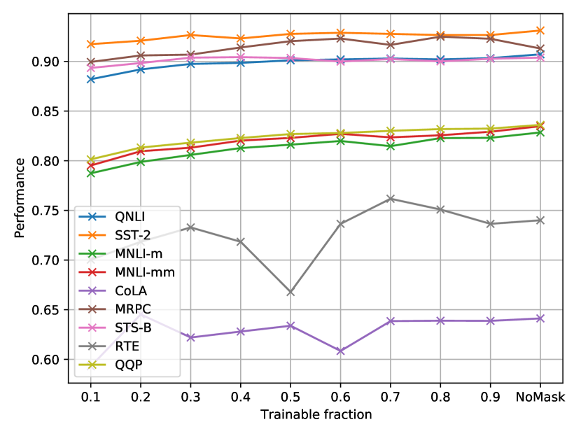
Figure 2: Validation results after training only a fraction of LayerNorm for different values of the trainable fraction.

3.3 Visualizing Fisher information of LayerNorm parameters

In this section, we visualize Fisher information of different parameters of LayerNorm in various tasks. We calculated the heat map of Fisher information of LayerNorm in different layers by summing the total Fisher information of each component. These heat maps are presented in Figure 3. Since LayerNorm has the weight and bias sub-components, we plotted them separately. The task is shown in the X-axis, and the Layer number is shown in Y-axis.

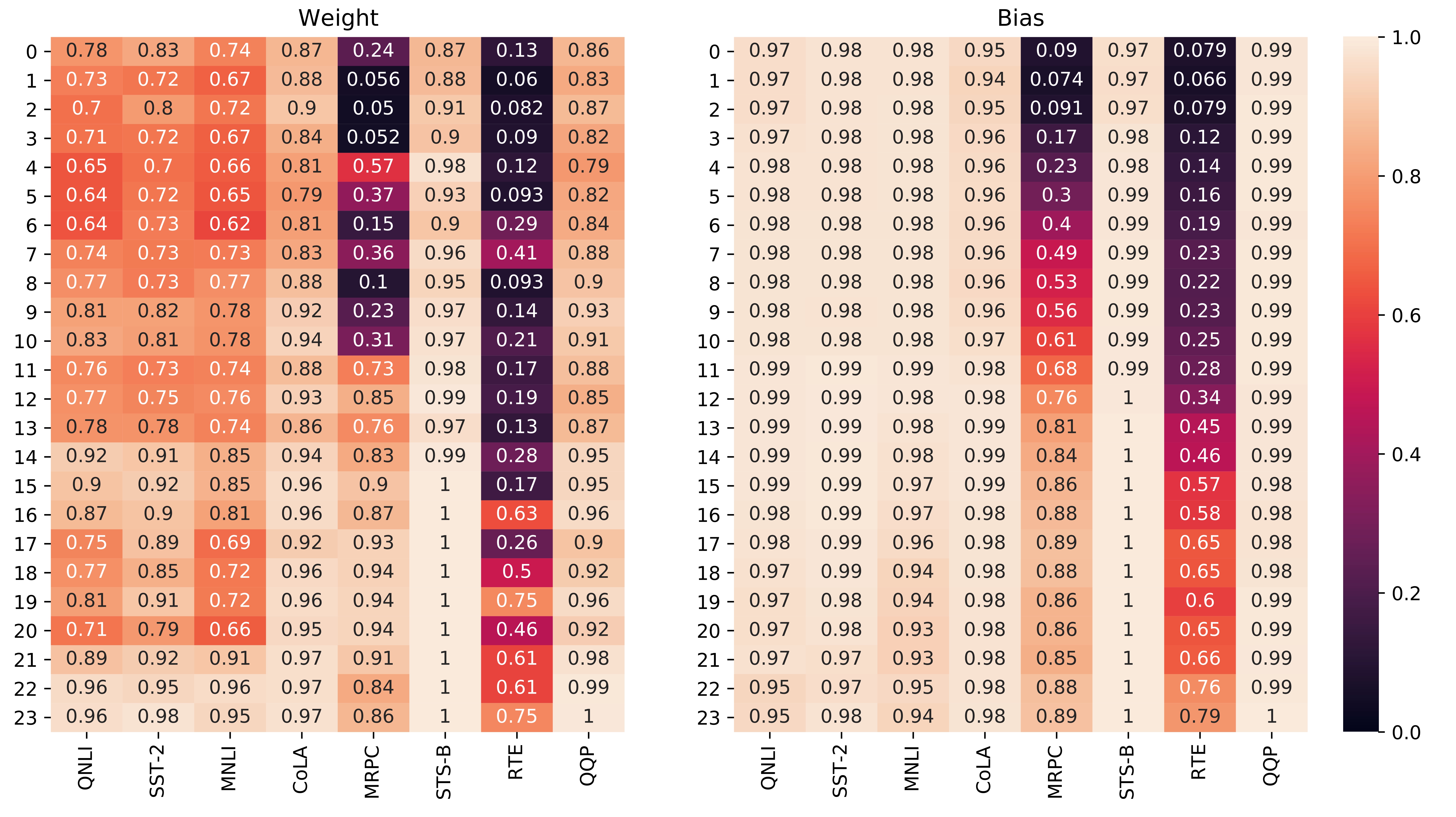
Figure 3: Heat map of Fisher information of LayerNorm in different layers. The X-axis is the task, the Y-axis is the Layer number.

Two findings can be observed from Figure 3: (1) the LayerNorm of BERT contains more information in the final layers than the initial layers, and (2) there is more information in the bias terms than the weights.

3.4 Global subset of LayerNorm

In section 3.2, we fine-tuned only a portion of LayerNorm for each task in the GLUE benchmark. However, for each task, we used a different subset of the network. In other words, the selected subset was task-specific. As an alternative, in this section, we used a single subset of the LayerNorm parameters for all the tasks to make the selected subset task-independent.

To find the global subset of the LayerNorm component, we calculated the Fisher information of each task separately, as described in section 3.2. Then, eight Fisher information, corresponding to eight tasks, were normalized by dividing the information of each task by its sum. This step was performed, because otherwise in one task, the total amount of information could be higher than other tasks, which would make the information of one task overshadowed by another task. After normalization, the Fisher information of all tasks were added to create a single global information matrix. The heat map of this information is presented in Figure 4. This global information was used to create masks with different densities as described in section 3.2. Validation results of training the model with the global subset of the LayerNorm are presented in Figure 5, as labeled as global. For the sake of comparison, for each task, we also plotted the results of running the algorithm using the individual (task-specific) masks, labeled as individual.

3.5 Cross-validating the subset of LayerNorm

In section 3.4, for each task, Fisher information of all eight tasks were used. To show that the global mask obtained is generalizable, we performed a cross-validation (CV) experiment: For each task, we used the Fisher information of all 7 other tasks to find the important subset of LayerNorm, excluding the target task itself. For example, the mask for MRPC was obtained by all tasks in GLUE except MRPC itself. In Figure 5, the results of these masks are labeled as CV. The good performance of CV indicates that the mask obtained from other tasks can be generalized to a new task.

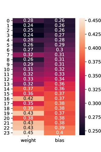
Figure 4: Heat map of Fisher information of LayerNorm in different layers. X-axis is the task and Y-axis is the Layer number. Left: Weight, right: Bias

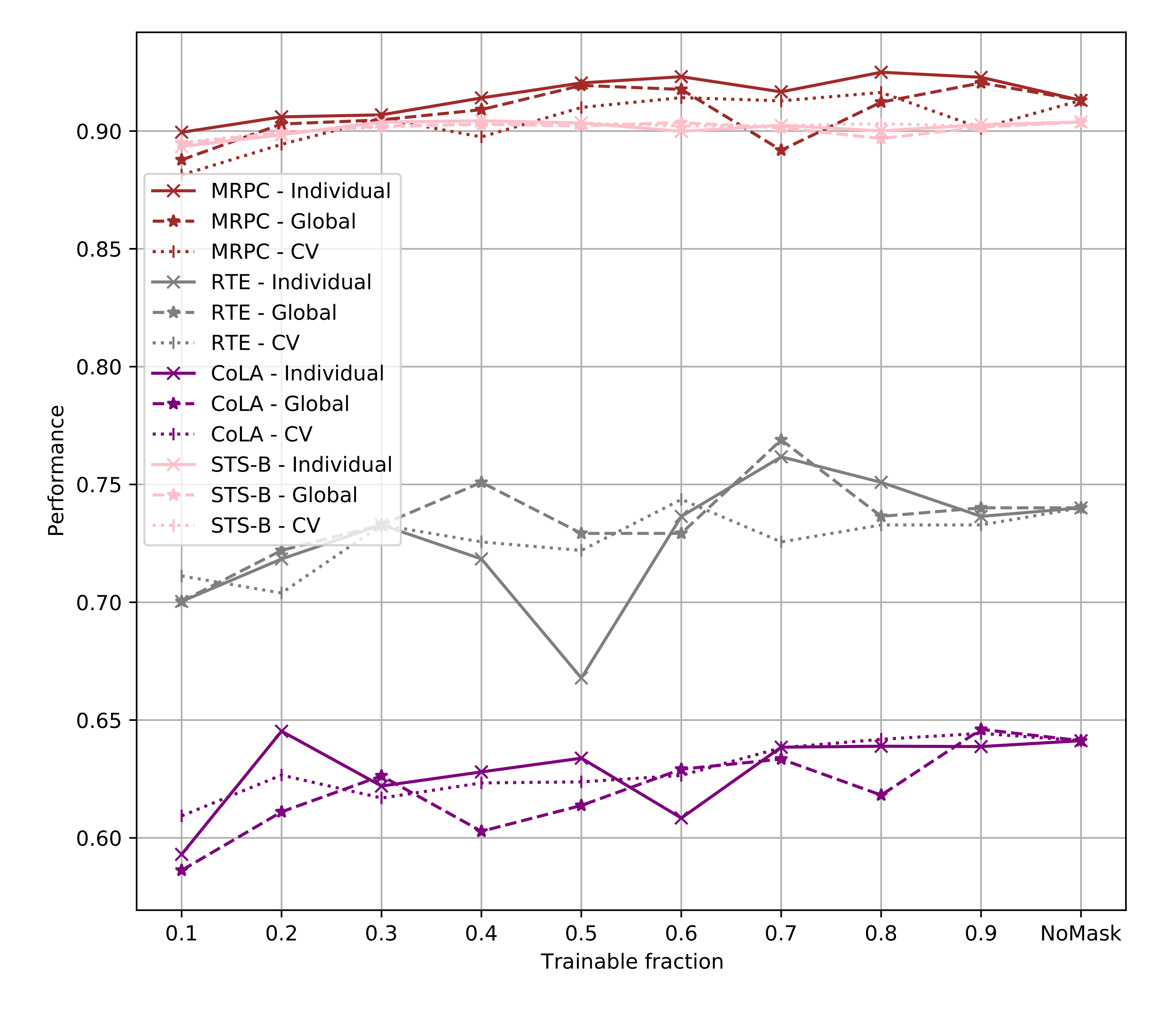
Figure 5: Validation results after training only a fixed fraction of LayerNorm for different values of the trainable fraction. For each task, the results of 3 experiments are plotted. Individual: The mask of each task is calculated based on information of that task. Global: The mask of each task is calculated based on information of all tasks. CV: The mask of each task has been calculated based on information of all tasks, excluding itself.

These results demonstrate that training a small subset of LayerNorm can achieve performance comparable to training the entire model. This is true even if the chosen subset is not task-specific, as observed in the global experiment, or when the subset is chosen without using the information of the task, as in the CV experiment.

4 Discussion

Although the Transformer-based models are robust against pruning (Michel et al., 2019; Gordon et al., 2020; Prasanna et al., 2020; Chen et al., 2020), Kovaleva et al. (2021) have demonstrated that the performance from the BERT family degrades significantly if LayerNorm is disabled in the model. This is consistent with our findings: Not only does LayerNorm undergo greater change than other components during the fine-tuning, but also training LayerNorm alone or a small portion of it has comparable performance to the fine-tuning of the full model or other components with a much larger size of parameters.

Each parameter in LayerNorm is multiplied by a weight and then a bias term is added to it. This indicates that the bias andhas the same size as the weight for this component. In Figure 3, we can see that for each task, bias terms have more information compared to the weight. This is consistent with the findings of (Zaken et al., 2021), where training only bias terms of BERT was proven to be effective.

In Figures 3 and 4 we observe that there is more information in the LayerNorm of the final layers of BERT and less information in the LayerNorm of the initial layers. This trend more or less exists in all the GLUE tasks. The higher Fisher information is, the larger gradient. As such, during the fine-tuning the final layers have larger gradient and will likely have more changes. This phenomenon has been observed in other studies (Merchant et al., 2020; Shi et al., 2022; ValizadehAslani et al., 2023).

5 Related work

In this section, we provide a brief overview of recent work related to parameter-efficient fine-tuning. In general, techniques proposed for parameter-efficient fine-tuning can be categorized into 5 groups: adding adaptors, adding prompts, model pruning, partial training, and low-rank decomposition. These groups are explained as follows.

Adding adaptors is to add trainable modules, called adaptors, into the original frozen model and only training the adaptors. Examples of such categories are Houlsby et al. (2019a); Guo et al. (2020); Mahabadi et al. (2021). Houlsby et al. (2019a) suggested injecting adapters between layers of the pre-trained network. Guo et al. (2020) proposed adding a sparse, task-specific difference-vector (diff-vector) to the pre-trained network.

Adding prompts involves prepended new tokens to the input text and only training the embeddings of these prompt tokens (Lester et al., 2021; Razdaibiedina et al., 2023). In such methods, the backpropagation is forced to apply the changes to the vectors corresponding to the soft prompt because the core model is frozen.

Model pruning is to remove certain weights from the network (LeCun et al., 1989; Hassibi et al., 1993; Han et al., 2015; Xia et al., 2022, 2023; Sun et al., 2024). To decide which weights should be pruned, Han et al. (2015) removed weights with low magnitude while Sun et al. (2024) evaluated each weight by the product of its magnitude and the norm of the corresponding input activation.

Partial training is only training a subset of the model (Lee et al., 2019; Zaken et al., 2021; Xu et al., 2021). Lee et al. (2019) only trained one-fourth of the final layers of BERT and RoBERTa. Zaken et al. (2021) suggested only fine-tuning the bias parameters. Xu et al. (2021) used Fisher information to select the most important parameters. Our proposed method falls within this category.

Low-rank decomposition methods utilize low-rank decomposition to approximate model update during fine-tuning (Hu et al., 2022; Zhang et al., 2023; Hyeon-Woo et al., 2022; Kopiczko et al., 2024; Liu et al., 2024). Hu et al. (2022) proposed Low-Rank Adaptation (LoRA). LoRA approximates the weight change of fine-tuning as the product of two low-rank matrices, where rather than training the whole model, only these low-rank matrices need to be trained. Liu et al. (2024) decomposed the pre-trained weight into two components, magnitude and direction, and used LoRA for the directional adaptation. These methods are similar to partial training because they apply a small modification to the weights of the pre-trained model.

6 Conclusions and future work

In this paper, we first examined all the components of BERT when fine-tuned for different GLUE tasks and showed that LayerNorm undergoes more changes after fine-tuning compared to other components. This is consistent with the findings of Kovaleva et al. (2021), where it was shown that, unlike other components, disabling LayerNorm has a dramatic negative effect on the performance of BERT. We then showed that only fine-tuning LayerNorm has a comparable performance to Bitfit, proposed by Zaken et al. (2021), in spite of being more sparse. Finally, using Fisher Information, we were able to select the important subsets of LayerNorm parameters and demonstrated that with slightly performance degradation, comparable results can be obtained by only fine-tuning as low as only 10% of LayerNorm parameters, which is one hundred thousandths of the BERT model.

In our analysis, we focused on the layer normalization, which is the popular method for normalization in the realm of NLP. However, in other fields, such as computer vision, batch normalization (see Appendix A) has been widely adopted (Shen et al., 2020). Applying the parameter-efficient training to batch-normalization can be employed as an extension of our work, and hence can make the training of batch-normalization models more computationally efficient.

Appendix A Normalization in neural networks

Generally, during the training of a deep neural network, adjustments in the parameters of a certain intermediate layer will cause a change in the distribution of the input to the next layer. This, phenomenon, called internal covariate shift, slows down the process of training by requiring a lower learning rate and a carful parameter initialization (Ioffe & Szegedy, 2015).

A.1 Batch normalization

One solution to this problem is batch normalization, which computes the mean and variance of the inputs to a neuron across a mini-batch of training examples. These statistics are then used to normalize the inputs to that neuron for each training sample. This simple modification makes the model robust against internal covariate shift and significantly reduces the training time (Ioffe & Szegedy, 2015).

A.1.1 Shortcomings of batch normalization

In spite of its effectiveness, batch normalization has multiple shortcomings:

1. Dependency on mini-batch size: Batch normalization relies on the mean and variance of the inputs across the mini-batch. This dependency can introduce significant variability in the normalization process, especially with small mini-batch sizes, which can be problematic for tasks that require small batches due to memory constraints (Ba et al., 2016a).

2. Performance in recurrent neural networks (RNNs): Batch normalization is less effective in RNNs due to the sequential nature of the data and the complications arising from applying normalization across time steps (Ba et al., 2016a).

3. Inference complications: Batch normalization requires maintaining running averages of the mean and variance during training to use for normalization during inference. This can complicate the model’s deployment, especially in models that see a significant shift in the input distribution at inference time. Unlike batch normalization, layer normalization carries out the same process at the training and inference phase (Ba et al., 2016a).

4. Batch Dependency: Since batch normalization normalizes inputs based on the batch’s statistics, it introduces a form of dependency between training examples within the batch. This can affect the model’s ability to generalize, especially for tasks where the independence of examples is crucial. This problem becomes particularly severe in NLP problems, where statistics of different batches are significantly different (Shen et al., 2020).

5. Inability to maintain criticality: In (Yang et al., 2019a), it was shown that batch normalization can cause gradient explosion. Generally, in a neural network, two undesired situations are exponentially growing co-variance and exponentially decaying covariance. The critical point between these two undesired situations is the point where the network has a perfect self-similarity of the co-variance and preserves it through the training from layer to layer (Roberts et al., 2021). This desired situation is called criticality (Roberts et al., 2021). Similar to Dropout (Schoenholz et al., 2017), batch normalization destroys criticality.

A.2 Layer Normalization (LayerNorm)

A.2.1 Description

Unlike, batch normalization, in LayerNorm, normalization is performed across the layer, not the batch, and all the hidden units in the same layer share the same normalization parameters for mean and variance (Song et al., 2023) (see Figure 6). As a result, normalization does not depend on the batch size and can be done with any batch size (including 1) (Ba et al., 2016a).

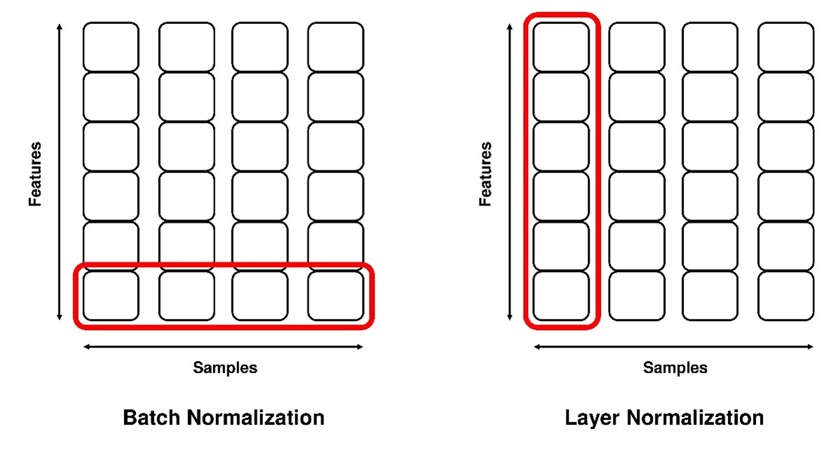
Figure 6: Unlike batch normalization, in layer normalization, normalization is performed across all features in the layer, not the same features in different samples of the batch..

LayerNorm works well in RNNs (Ba et al., 2016a). Additionally, the process of layer normalization is exactly the same in training and inference (Ba et al., 2016a). Unlike batch normalization, which destroys criticality, LayerNorm, maintains criticality because proper stacking of LayerNorm leads to an architecture that is critical for any initialization (Doshi et al., 2023). It was demonstrated by Xiong et al. (2020) that LayerNorm plays a crucial role in controlling the gradient scales and the effect of the location of LayerNorm on the gradient was investigated. In (Shleifer & Ott, 2022), the problem of uneven gradient magnitude mismatch in different layers was mitigated by adding 3 normalization operators to each layer. Alternative versions of LayerNorm have also been proposed to improve gradient propagation (Shen et al., 2020), (Xu et al., 2019), (Wang et al., 2020). Xu et al. (2019) suggested removing bias and gain parameters of LayerNorm to prevent over-fitting. Wang et al. (2020) proposed variance-only LayerNorm, where normalization is done without subtracting the mean in equation (4). LayerNorm has also been employed in RNNs (Wei, 2021). Next, a more technical description of LayerNorm is provided.

A.2.2 Technical details

LayerNorm normalizes the outputs of both self-attention and linear layers (Ba et al., 2016b). For an input of the $i$-th layer, $\mathbf{x_{i}}$, of size $H$, where each element is represented by $x_{ij}$, LayerNorm first computes mean $\mu_{i}$ and variance ${\sigma_{i}}^{2}$ across the features:

$$\mu_{i}=\frac{1}{H}\sum_{j=1}^{H}{x_{ij}},\;\;{\sigma_{i}}^{2}=\frac{1}{H}\sum_{j=1}^{H}{({x_{ij}-\mu_{i}})^{2}}$$ (3)

After calculating the above values, the inputs are normalized based on these values:

$$\hat{x}_{ij}=\frac{x_{ij}-\mu_{i}}{\sqrt{\sigma^{2}+\epsilon}}$$ (4)

Note that $\epsilon$ is only used to avoid zero-division. Then, the normalized value go through an affine transformation, which contains the learnable parameters $\boldsymbol{\omega}$ and bias $\mathbf{b}$:

$$\mathbf{y_{i}}=\boldsymbol{\omega}\odot\mathbf{\hat{x}_{i}}+\mathbf{b}$$ (5)

where $\odot$ is Hadamard (element-wise) multiplication.

Appendix B Distance definitions

For 2 vectors, like $V_{1}$, and $V_{2}$, of size $n$, $L_{0}$ distance is defined as the number of non-zero elements in ${V_{1}}_{i}-{V_{2}}_{i}$ where $i$ indicates element index. This is a similar idea to Hamming distance (Waggener, 1995).

$L_{1}$, or Manhattan, distance, between 2 such vectors is defined as:

$$L_{1}=\sum_{i=1}^{n}|{V_{1}}_{i}-{V_{2}}_{i}|$$ (6)

Appendix C Metrics for GLUE results

Table 4 shows the metric used for each task.

Table 4: Metrics used to evaluate GLUE Benchmark.

Task	Metric
QNLI	accuracy
SST-2	accuracy
MNLI	Matched accuracy/mismatched accuracy
CoLA	Matthews correlation
MRPC	F1
STS-B	Spearman correlation
RTE	accuracy
QQP	F1

References

- GLU (2021) Glue. https://gluebenchmark.com/, 2021. Accessed: 2021-11-03.
- Aghajanyan et al. (2021) Armen Aghajanyan, Akshat Shrivastava, Anchit Gupta, Naman Goyal, Luke Zettlemoyer, and Sonal Gupta. Better fine-tuning by reducing representational collapse. In International Conference on Learning Representations, 2021. URL https://openreview.net/forum?id=OQ08SN70M1V.
- Ba et al. (2016a) Jimmy Lei Ba, Jamie Ryan Kiros, and Geoffrey E. Hinton. Layer normalization, 2016a.
- Ba et al. (2016b) Jimmy Lei Ba, Jamie Ryan Kiros, and Geoffrey E. Hinton. Layer normalization, 2016b.
- Bar-Haim et al. (2006) Roy Bar-Haim, Ido Dagan, Bill Dolan, Lisa Ferro, Danilo Giampiccolo, and Bernardo Magnini. The second pascal recognising textual entailment challenge. 2006.
- Bentivogli et al. (2009) Luisa Bentivogli, Ido Dagan, Hoa Trang Dang, Danilo Giampiccolo, and Bernardo Magnini. The fifth pascal recognizing textual entailment challenge. In In Proc Text Analysis Conference (TAC’09, 2009.
- Cer et al. (2017) Daniel Cer, Mona Diab, Eneko Agirre, Iñigo Lopez-Gazpio, and Lucia Specia. SemEval-2017 task 1: Semantic textual similarity multilingual and crosslingual focused evaluation. In Proceedings of the 11th International Workshop on Semantic Evaluation (SemEval-2017), pp. 1–14, Vancouver, Canada, August 2017. Association for Computational Linguistics. doi:10.18653/v1/S17-2001. URL https://aclanthology.org/S17-2001.
- Chen et al. (2020) Tianlong Chen, Jonathan Frankle, Shiyu Chang, Sijia Liu, Yang Zhang, Zhangyang Wang, and Michael Carbin. The lottery ticket hypothesis for pre-trained bert networks, 2020.
- Dagan et al. (2006) Ido Dagan, Oren Glickman, and Bernardo Magnini. The pascal recognising textual entailment challenge. In Joaquin Quiñonero-Candela, Ido Dagan, Bernardo Magnini, and Florence d’Alché Buc (eds.), Machine Learning Challenges. Evaluating Predictive Uncertainty, Visual Object Classification, and Recognising Tectual Entailment, pp. 177–190, Berlin, Heidelberg, 2006. Springer Berlin Heidelberg. ISBN 978-3-540-33428-6.
- Devlin et al. (2018) Jacob Devlin, Ming-Wei Chang, Kenton Lee, and Kristina Toutanova. BERT: pre-training of deep bidirectional transformers for language understanding. CoRR, abs/1810.04805, 2018. URL http://arxiv.org/abs/1810.04805.
- Devlin et al. (2019) Jacob Devlin, Ming-Wei Chang, Kenton Lee, and Kristina Toutanova. BERT: Pre-training of deep bidirectional transformers for language understanding. In Proceedings of the 2019 Conference of the North American Chapter of the Association for Computational Linguistics: Human Language Technologies, Volume 1 (Long and Short Papers), pp. 4171–4186, Minneapolis, Minnesota, June 2019. Association for Computational Linguistics. doi:10.18653/v1/N19-1423. URL https://aclanthology.org/N19-1423.
- Dolan & Brockett (2005) William B. Dolan and Chris Brockett. Automatically constructing a corpus of sentential paraphrases. In Proceedings of the Third International Workshop on Paraphrasing (IWP2005), 2005. URL https://aclanthology.org/I05-5002.
- Doshi et al. (2023) Darshil Doshi, Tianyu He, and Andrey Gromov. Critical initialization of wide and deep neural networks through partial jacobians: General theory and applications, 2023. URL https://openreview.net/forum?id=xb333aboIu.
- Giampiccolo et al. (2007) Danilo Giampiccolo, Bernardo Magnini, Ido Dagan, and Bill Dolan. The third PASCAL recognizing textual entailment challenge. In Proceedings of the ACL-PASCAL Workshop on Textual Entailment and Paraphrasing, pp. 1–9, Prague, June 2007. Association for Computational Linguistics. URL https://aclanthology.org/W07-1401.
- Gordon et al. (2020) Mitchell Gordon, Kevin Duh, and Nicholas Andrews. Compressing BERT: Studying the effects of weight pruning on transfer learning. In Proceedings of the 5th Workshop on Representation Learning for NLP. Association for Computational Linguistics, 2020. doi:10.18653/v1/2020.repl4nlp-1.18. URL https://doi.org/10.18653/v1/2020.repl4nlp-1.18.
- Guo et al. (2020) Demi Guo, Alexander M. Rush, and Yoon Kim. Parameter-efficient transfer learning with diff pruning, 2020.
- Han et al. (2015) Song Han, Jeff Pool, John Tran, and William J. Dally. Learning both weights and connections for efficient neural network. In Neural Information Processing Systems, 2015. URL https://api.semanticscholar.org/CorpusID:2238772.
- Hassibi et al. (1993) B. Hassibi, D.G. Stork, and G.J. Wolff. Optimal brain surgeon and general network pruning. In IEEE International Conference on Neural Networks, pp. 293–299 vol.1, 1993. doi:10.1109/ICNN.1993.298572.
- Houlsby et al. (2019a) Neil Houlsby, Andrei Giurgiu, Stanislaw Jastrzebski, Bruna Morrone, Quentin de Laroussilhe, Andrea Gesmundo, Mona Attariyan, and Sylvain Gelly. Parameter-efficient transfer learning for NLP. CoRR, abs/1902.00751, 2019a. URL http://arxiv.org/abs/1902.00751.
- Houlsby et al. (2019b) Neil Houlsby, Andrei Giurgiu, Stanislaw Jastrzebski, Bruna Morrone, Quentin de Laroussilhe, Andrea Gesmundo, Mona Attariyan, and Sylvain Gelly. Parameter-efficient transfer learning for nlp, 2019b.
- Hu et al. (2022) Edward J Hu, yelong shen, Phillip Wallis, Zeyuan Allen-Zhu, Yuanzhi Li, Shean Wang, Lu Wang, and Weizhu Chen. LoRA: Low-rank adaptation of large language models. In International Conference on Learning Representations, 2022. URL https://openreview.net/forum?id=nZeVKeeFYf9.
- Hyeon-Woo et al. (2022) Nam Hyeon-Woo, Moon Ye-Bin, and Tae-Hyun Oh. Fedpara: Low-rank hadamard product for communication-efficient federated learning. In International Conference on Learning Representations, 2022. URL https://openreview.net/forum?id=d71n4ftoCBy.
- Ioffe & Szegedy (2015) Sergey Ioffe and Christian Szegedy. Batch normalization: Accelerating deep network training by reducing internal covariate shift. In Francis Bach and David Blei (eds.), Proceedings of the 32nd International Conference on Machine Learning, volume 37 of Proceedings of Machine Learning Research, pp. 448–456, Lille, France, 07–09 Jul 2015. PMLR. URL https://proceedings.mlr.press/v37/ioffe15.html.
- Iyer et al. (2017) Shankar Iyer, Nikhil Dandekar, and Kornél Csernai. First quora dataset release: Question pairs., 2017.
- Kirkpatrick et al. (2016) James Kirkpatrick, Razvan Pascanu, Neil C. Rabinowitz, Joel Veness, Guillaume Desjardins, Andrei A. Rusu, Kieran Milan, John Quan, Tiago Ramalho, Agnieszka Grabska-Barwinska, Demis Hassabis, Claudia Clopath, Dharshan Kumaran, and Raia Hadsell. Overcoming catastrophic forgetting in neural networks. CoRR, abs/1612.00796, 2016. URL http://arxiv.org/abs/1612.00796.
- Kopiczko et al. (2024) Dawid Jan Kopiczko, Tijmen Blankevoort, and Yuki M Asano. ELoRA: Efficient low-rank adaptation with random matrices. In The Twelfth International Conference on Learning Representations, 2024. URL https://openreview.net/forum?id=NjNfLdxr3A.
- Kovaleva et al. (2021) Olga Kovaleva, Saurabh Kulshreshtha, Anna Rogers, and Anna Rumshisky. Bert busters: Outlier dimensions that disrupt transformers, 2021.
- Kruskal & Wallis (1952) William H. Kruskal and W. Allen Wallis. Use of ranks in one-criterion variance analysis. Journal of the American Statistical Association, 47(260):583–621, December 1952. doi:10.1080/01621459.1952.10483441. URL https://doi.org/10.1080/01621459.1952.10483441.
- LeCun et al. (1989) Yann LeCun, John Denker, and Sara Solla. Optimal brain damage. In D. Touretzky (ed.), Advances in Neural Information Processing Systems, volume 2. Morgan-Kaufmann, 1989. URL https://proceedings.neurips.cc/paper_files/paper/1989/file/6c9882bbac1c7093bd25041881277658-Paper.pdf.
- Lee et al. (2019) Jaejun Lee, Raphael Tang, and Jimmy J. Lin. What would elsa do? freezing layers during transformer fine-tuning. ArXiv, abs/1911.03090, 2019. URL https://api.semanticscholar.org/CorpusID:207847573.
- Lester et al. (2021) Brian Lester, Rami Al-Rfou, and Noah Constant. The power of scale for parameter-efficient prompt tuning. In Marie-Francine Moens, Xuanjing Huang, Lucia Specia, and Scott Wen-tau Yih (eds.), Proceedings of the 2021 Conference on Empirical Methods in Natural Language Processing, pp. 3045–3059, Online and Punta Cana, Dominican Republic, November 2021. Association for Computational Linguistics. doi:10.18653/v1/2021.emnlp-main.243. URL https://aclanthology.org/2021.emnlp-main.243.
- Levesque et al. (2012) Hector J. Levesque, Ernest Davis, and Leora Morgenstern. The winograd schema challenge. In 13th International Conference on the Principles of Knowledge Representation and Reasoning, KR 2012, Proceedings of the International Conference on Knowledge Representation and Reasoning, pp. 552–561. Institute of Electrical and Electronics Engineers Inc., 2012. ISBN 9781577355601. 13th International Conference on the Principles of Knowledge Representation and Reasoning, KR 2012 ; Conference date: 10-06-2012 Through 14-06-2012.
- Liu et al. (2024) Shih-Yang Liu, Chien-Yi Wang, Hongxu Yin, Pavlo Molchanov, Yu-Chiang Frank Wang, Kwang-Ting Cheng, and Min-Hung Chen. Dora: Weight-decomposed low-rank adaptation, 2024.
- Liu et al. (2019) Yinhan Liu, Myle Ott, Naman Goyal, Jingfei Du, Mandar Joshi, Danqi Chen, Omer Levy, Mike Lewis, Luke Zettlemoyer, and Veselin Stoyanov. Roberta: A robustly optimized bert pretraining approach, 2019.
- mahabadi et al. (2021) Rabeeh Karimi mahabadi, Yonatan Belinkov, and James Henderson. Variational information bottleneck for effective low-resource fine-tuning. In International Conference on Learning Representations, 2021. URL https://openreview.net/forum?id=kvhzKz-_DMF.
- Mahabadi et al. (2021) Rabeeh Karimi Mahabadi, Sebastian Ruder, Mostafa Dehghani, and James Henderson. Parameter-efficient multi-task fine-tuning for transformers via shared hypernetworks. In Annual Meeting of the Association for Computational Linguistics, 2021. URL https://api.semanticscholar.org/CorpusID:235309789.
- Merchant et al. (2020) Amil Merchant, Elahe Rahimtoroghi, Ellie Pavlick, and Ian Tenney. What happens to BERT embeddings during fine-tuning? CoRR, abs/2004.14448, 2020. URL https://arxiv.org/abs/2004.14448.
- Merity et al. (2016) Stephen Merity, Caiming Xiong, James Bradbury, and Richard Socher. Pointer sentinel mixture models, 2016.
- Michel et al. (2019) Paul Michel, Omer Levy, and Graham Neubig. Are sixteen heads really better than one? In H. Wallach, H. Larochelle, A. Beygelzimer, F. d'Alché-Buc, E. Fox, and R. Garnett (eds.), Advances in Neural Information Processing Systems, volume 32. Curran Associates, Inc., 2019. URL https://proceedings.neurips.cc/paper/2019/file/2c601ad9d2ff9bc8b282670cdd54f69f-Paper.pdf.
- Mikolov et al. (2013) Tomas Mikolov, Ilya Sutskever, Kai Chen, Greg S Corrado, and Jeff Dean. Distributed representations of words and phrases and their compositionality. In C. J. C. Burges, L. Bottou, M. Welling, Z. Ghahramani, and K. Q. Weinberger (eds.), Advances in Neural Information Processing Systems, volume 26. Curran Associates, Inc., 2013. URL https://proceedings.neurips.cc/paper/2013/file/9aa42b31882ec039965f3c4923ce901b-Paper.pdf.
- Pennington et al. (2014) Jeffrey Pennington, Richard Socher, and Christopher Manning. GloVe: Global vectors for word representation. In Proceedings of the 2014 Conference on Empirical Methods in Natural Language Processing (EMNLP), pp. 1532–1543, Doha, Qatar, October 2014. Association for Computational Linguistics. doi:10.3115/v1/D14-1162. URL https://aclanthology.org/D14-1162.
- Prasanna et al. (2020) Sai Prasanna, Anna Rogers, and Anna Rumshisky. When BERT plays the lottery, all tickets are winning. In Proceedings of the 2020 Conference on Empirical Methods in Natural Language Processing (EMNLP). Association for Computational Linguistics, 2020. doi:10.18653/v1/2020.emnlp-main.259. URL https://doi.org/10.18653/v1/2020.emnlp-main.259.
- Radiya-Dixit & Wang (2020) Evani Radiya-Dixit and Xin Wang. How fine can fine-tuning be? learning efficient language models, 2020.
- Rajpurkar et al. (2016) Pranav Rajpurkar, Jian Zhang, Konstantin Lopyrev, and Percy Liang. SQuAD: 100,000+ questions for machine comprehension of text. In Proceedings of the 2016 Conference on Empirical Methods in Natural Language Processing, pp. 2383–2392, Austin, Texas, November 2016. Association for Computational Linguistics. doi:10.18653/v1/D16-1264. URL https://aclanthology.org/D16-1264.
- Razdaibiedina et al. (2023) Anastasia Razdaibiedina, Yuning Mao, Rui Hou, Madian Khabsa, Mike Lewis, Jimmy Ba, and Amjad Almahairi. Residual prompt tuning: Improving prompt tuning with residual reparameterization. In Proceedings of the 61st Annual Meeting of the Association for Computational Linguistics, 2023.
- Roberts et al. (2021) Daniel A. Roberts, Sho Yaida, and Boris Hanin. The principles of deep learning theory. CoRR, abs/2106.10165, 2021. URL https://arxiv.org/abs/2106.10165.
- Schoenholz et al. (2017) Samuel S. Schoenholz, Justin Gilmer, Surya Ganguli, and Jascha Sohl-Dickstein. Deep information propagation. In International Conference on Learning Representations, 2017. URL https://openreview.net/forum?id=H1W1UN9gg.
- Shen et al. (2020) Sheng Shen, Zhewei Yao, Amir Gholami, Michael W. Mahoney, and Kurt Keutzer. Powernorm: rethinking batch normalization in transformers. In Proceedings of the 37th International Conference on Machine Learning, ICML’20. JMLR.org, 2020.
- Shi et al. (2022) Yiwen Shi, Jing Wang, Ping Ren, Taha ValizadehAslani, Yi Zhang, Meng Hu, and Hualou Liang. Fine-tuning bert for automatic adme semantic labeling in fda drug labeling to enhance product-specific guidance assessment, 2022.
- Shleifer & Ott (2022) Sam Shleifer and Myle Ott. Normformer: Improved transformer pretraining with extra normalization, 2022. URL https://openreview.net/forum?id=GMYWzWztDx5.
- Socher et al. (2013) Richard Socher, Alex Perelygin, Jean Wu, Jason Chuang, Christopher D. Manning, Andrew Ng, and Christopher Potts. Recursive deep models for semantic compositionality over a sentiment treebank. In Proceedings of the 2013 Conference on Empirical Methods in Natural Language Processing, pp. 1631–1642, Seattle, Washington, USA, October 2013. Association for Computational Linguistics. URL https://aclanthology.org/D13-1170.
- Song et al. (2023) Jia Song, A-Xing Zhu, and Yunqiang Zhu. Transformer-based semantic segmentation for extraction of building footprints from very-high-resolution images. Sensors, 23(11), 2023. ISSN 1424-8220. doi:10.3390/s23115166. URL https://www.mdpi.com/1424-8220/23/11/5166.
- Sun et al. (2024) Mingjie Sun, Zhuang Liu, Anna Bair, and J Zico Kolter. A simple and effective pruning approach for large language models. In The Twelfth International Conference on Learning Representations, 2024. URL https://openreview.net/forum?id=PxoFut3dWW.
- Tu et al. (2016) Ming Tu, Visar Berisha, Yu Cao, and Jae-Sun Seo. Reducing the model order of deep neural networks using information theory. In 2016 IEEE Computer Society Annual Symposium on VLSI (ISVLSI). IEEE, July 2016. doi:10.1109/isvlsi.2016.117. URL https://doi.org/10.1109/isvlsi.2016.117.
- ValizadehAslani et al. (2023) Taha ValizadehAslani, Yiwen Shi, Ping Ren, Jing Wang, Yi Zhang, Meng Hu, Liang Zhao, and Hualou Liang. PharmBERT: a domain-specific BERT model for drug labels. Briefings in Bioinformatics, 24(4):bbad226, 06 2023. ISSN 1477-4054. doi:10.1093/bib/bbad226. URL https://doi.org/10.1093/bib/bbad226.
- Vaswani et al. (2017) Ashish Vaswani, Noam Shazeer, Niki Parmar, Jakob Uszkoreit, Llion Jones, Aidan N Gomez, Ł ukasz Kaiser, and Illia Polosukhin. Attention is all you need. In I. Guyon, U. V. Luxburg, S. Bengio, H. Wallach, R. Fergus, S. Vishwanathan, and R. Garnett (eds.), Advances in Neural Information Processing Systems, volume 30. Curran Associates, Inc., 2017. URL https://proceedings.neurips.cc/paper/2017/file/3f5ee243547dee91fbd053c1c4a845aa-Paper.pdf.
- Waggener (1995) William Waggener. Pulse code modulation techniques : with applications in communications and data recording. Van Nostrand Reinhold, New York, 1995. ISBN 9780442014360.
- Wang et al. (2019) Alex Wang, Amanpreet Singh, Julian Michael, Felix Hill, Omer Levy, and Samuel R. Bowman. Glue: A multi-task benchmark and analysis platform for natural language understanding, 2019.
- Wang et al. (2020) Zhiqiang Wang, Qingyun She, Pengtao Zhang, and Junlin Zhang. Correct normalization matters: Understanding the effect of normalization on deep neural network models for click-through rate prediction. CoRR, abs/2006.12753, 2020. URL https://arxiv.org/abs/2006.12753.
- Warstadt et al. (2019) Alex Warstadt, Amanpreet Singh, and Samuel R. Bowman. Neural Network Acceptability Judgments. Transactions of the Association for Computational Linguistics, 7:625–641, 09 2019. ISSN 2307-387X. doi:10.1162/tacl_a_00290. URL https://doi.org/10.1162/tacl_a_00290.
- Wei (2021) Siheng Wei. Distantly supervision for relation extraction via layernorm gated recurrent neural networks. In 2021 2nd International Conference on Computing and Data Science (CDS), pp. 94–99, 2021. doi:10.1109/CDS52072.2021.00022.
- Williams et al. (2018) Adina Williams, Nikita Nangia, and Samuel Bowman. A broad-coverage challenge corpus for sentence understanding through inference. In Proceedings of the 2018 Conference of the North American Chapter of the Association for Computational Linguistics: Human Language Technologies, Volume 1 (Long Papers), pp. 1112–1122, New Orleans, Louisiana, June 2018. Association for Computational Linguistics. doi:10.18653/v1/N18-1101. URL https://aclanthology.org/N18-1101.
- Xia et al. (2022) Mengzhou Xia, Zexuan Zhong, and Danqi Chen. Structured pruning learns compact and accurate models. ArXiv, abs/2204.00408, 2022. URL https://api.semanticscholar.org/CorpusID:247922354.
- Xia et al. (2023) Mengzhou Xia, Tianyu Gao, Zhiyuan Zeng, and Danqi Chen. Sheared LLaMA: Accelerating language model pre-training via structured pruning. In Workshop on Advancing Neural Network Training: Computational Efficiency, Scalability, and Resource Optimization (WANT@NeurIPS 2023), 2023. URL https://openreview.net/forum?id=6s77hjBNfS.
- Xiong et al. (2020) Ruibin Xiong, Yunchang Yang, Di He, Kai Zheng, Shuxin Zheng, Huishuai Zhang, Yanyan Lan, Liwei Wang, and Tie-Yan Liu. On layer normalization in the transformer architecture, 2020. URL https://openreview.net/forum?id=B1x8anVFPr.
- Xu et al. (2019) Jingjing Xu, Xu Sun, Zhiyuan Zhang, Guangxiang Zhao, and Junyang Lin. Understanding and improving layer normalization. CoRR, abs/1911.07013, 2019. URL http://arxiv.org/abs/1911.07013.
- Xu et al. (2021) Runxin Xu, Fuli Luo, Zhiyuan Zhang, Chuanqi Tan, Baobao Chang, Songfang Huang, and Fei Huang. Raise a child in large language model: Towards effective and generalizable fine-tuning, 2021.
- Yang et al. (2019a) Greg Yang, Jeffrey Pennington, Vinay Rao, Jascha Sohl-Dickstein, and Samuel S. Schoenholz. A mean field theory of batch normalization. In International Conference on Learning Representations, 2019a. URL https://openreview.net/forum?id=SyMDXnCcF7.
- Yang et al. (2019b) Zhilin Yang, Zihang Dai, Yiming Yang, Jaime Carbonell, Ruslan Salakhutdinov, and Quoc V. Le. Xlnet: Generalized autoregressive pretraining for language understanding, 2019b.
- Zaken et al. (2021) Elad Ben Zaken, Shauli Ravfogel, and Yoav Goldberg. Bitfit: Simple parameter-efficient fine-tuning for transformer-based masked language-models, 2021.
- Zhang et al. (2023) Qingru Zhang, Minshuo Chen, Alexander Bukharin, Nikos Karampatziakis, Pengcheng He, Yu Cheng, Weizhu Chen, and Tuo Zhao. Adalora: Adaptive budget allocation for parameter-efficient fine-tuning, 2023.
- Zhao et al. (2019) Sanqiang Zhao, Raghav Gupta, Yang Song, and Denny Zhou. Extremely small bert models from mixed-vocabulary training, 2019.