Quantum critical engine at finite temperatures

Abstract

We construct a quantum critical Otto engine that is powered by finite temperature baths. We show that the work output of the engine shows universal power law behavior that depends on the critical exponents of the working medium, as well as on the temperature of the cold bath. Furthermore, higher temperatures of the cold bath allows the engine to approach the limit of adiabatic operation for smaller values of the time period, while the corresponding power shows a maximum at an intermediate value of the cold bath temperature. These counterintuitive results stems from thermal excitations dominating the dynamics at higher temperatures.

1 Introduction

Quantum thermodynamics is a rapidly progressing field aimed at understanding the thermodynamics at the quantum level [1, 2]. The field is getting much attention from the scientific community not just because it provides a link between quantum mechanics and thermodynamics but also because it aids in the development of nanoscale devices that aims to harness the potential benefits of the “quantumness" in their working medium (WM) [3]. The recent advances in the experiments such as trapped ions or ultracold atoms [4, 5], using NMR techniques [6], nitrogen vacancy centres in diamond [7] have made the realization of quantum devices possible. Among the various quantum devices studied, for example, quantum refrigerators [8, 9], quantum batteries [10, 11], quantum sensors [12], quantum thermal transistors [13, 14], etc., our work focusses on quantum heat engines that follow the quantum Otto cycle [15, 16].

The effect of phase transitions in quantum engines has been studied in Refs. [17, 18, 19, 20, 21, 22, 23, 24]. While some of these studies concentrated on how to improve the performance of quantum engines with respect to its efficiency and power [23, 24], some focussed on showcasing universality in their working [22, 21]. For instance, in Ref. [22], the authors showed that the work output of the engine up to an additive constant follows a universal power law governed by the driving speed with which the quantum critical points are crossed, where the exponent of the power law is determined by the critical points (CP) crossed. However, they considered the case of relaxing bath that takes the WM close to its ground state so that Kibble Zurek mechanism becomes relevant. On the other hand, in this paper, we specifically use thermal baths at different temperatures and study the effect of thermal excitations on the scalings of the work output. As discussed before, we prepare a many body quantum heat engine using a free fermionic model as WM that undergoes a quantum phase transition. We describe the details of the free fermionic model in Section 2, elaborate on the many body quantum Otto cycle that the engine follows in Section 3, followed by the universal scalings shown by the engine in Section 4. We demonstrate our results using the transverse field Ising model in Section 5 and finally conclude in Section 6.

2 Free fermionic model

Let us consider a free fermionic model described by the Hamiltonian

$$H=\sum_{k}\psi_{k}^{\dagger}H_{k}\psi_{k},$$ (1)

with $H_{k}$ taking the form

$$H_{k}=(\alpha+m_{k})\sigma^{z}+n_{k}\sigma^{x}.$$ (2)

Here, $\sigma^{i}$ ($i=x,y,z$) are the Pauli matrices, $\psi_{k}=(c_{1k},c_{2k})$ where $c_{jk}(j=1,2)$ are the fermionic operators corresponding to the $k$-th momentum mode. The parameters $\alpha,m_{k}$ and $n_{k}$ depend on the specific model that one works on, say Ising [25], X-Y [26] or Kitaev model [27]. The energy gap between the ground state and the first excited state is given by $\Delta_{k}=2\sqrt{(\alpha+m_{k})^{2}+|n_{k}|^{2}}$. This Hamiltonian shows a quantum phase transition at the quantum critical point where the energy gap $\Delta_{k}$ vanishes for the critical mode $k=k_{c}$ for certain combinations of $\alpha,~{}m_{k}$ and $n_{k}$.

With each momentum mode being independent and non-interacting, we can write the density matrix of the system as

$$\rho=\otimes_{k}\rho_{k},$$ (3)

where $\rho_{k}$ is written in the basis $|0_{1k},0_{2k}\rangle,|1_{1k},0_{2k}\rangle,|0_{1k},1_{2k}\rangle$ and $|1_{1k},1_{2k}\rangle$ so that the first index corresponds to presence (1) or absence (0) of $c_{1k}$ fermions, which is also the case for second index related to $c_{2k}$ fermions. It is to be noted that since the non-unitary dynamics mixes all four basis, we need to rewrite the Hamiltonian $H_{k}$ in these four basis leading to [28, 29]

$$H_{k}=\begin{bmatrix}(\alpha+m_{k})&0&0&n_{k}\\ 0&0&0&0\\ 0&0&0&0\\ n_{k}&0&0&-(\alpha+m_{k})\end{bmatrix},$$ (4)

whose eigenvalues are $-\epsilon_{k},0,0,\epsilon_{k}$ where $\epsilon_{k}=\Delta_{k}/2=\sqrt{(\alpha+m_{k})^{2}+|n_{k}|^{2}}$.

3 Many body quantum Otto cycle

We now describe the quantum Otto cycle (QOC) which consist of four strokes (also shown in Fig.1):

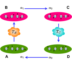
Figure 1: Schematic diagram of a quantum Otto cycle

• Stroke A $\rightarrow$ B: The WM with parameter $\alpha=\alpha_{1}$ is connected to the hot bath at a temperature $T_{H}$ for a time $\tau_{H}$ so that it reaches the thermal state at B given by

  $$\rho_{k}^{B}=\begin{bmatrix}\frac{e^{\beta_{H}\epsilon_{k}}}{Z_{H}}&0&0&0\\ 0&\frac{1}{Z_{H}}&0&0\\ 0&0&\frac{1}{Z_{H}}&0\\ 0&0&0&\frac{e^{-\beta_{H}\epsilon_{k}}}{Z_{H}}\end{bmatrix}.$$ (5)

  Here $\beta_{H}=\frac{1}{k_{B}T_{H}}$, (we have set $k_{B}=1$ throughout this article) and $Z_{H}=2+e^{\beta_{H}\epsilon_{k}}+e^{-\beta_{H}\epsilon_{k}}$ is the partition function for each mode $k$ with $\epsilon_{k}$ as the energy when $\alpha=\alpha_{1}$. The energy exchanged in this stroke is denoted by $\mathcal{Q}_{in}$.
  

• Stroke B $\rightarrow$ C: The WM is disconnected from the hot bath and $\alpha$ is changed from $\alpha_{1}$ to $\alpha_{2}$ using the driving protocol,

  $$\alpha(t)=\alpha_{1}+(\alpha_{2}-\alpha_{1})(\frac{t}{\tau_{1}}),\hskip 8.5359ptt\in[0,\tau_{1}].$$ (6)

  The evolution being a unitary evolution is given by the von-Neumann equation of motion:

  $$\frac{d\rho_{k}}{dt}=-i[H_{k},\rho_{k}].$$ (7)

  In this work, we shall focus on $\alpha_{2}=\alpha_{c}$, the critical value, for the reasons that will be explained later.
  

• Stroke C $\rightarrow$ D: The WM with $\alpha=\alpha_{2}$ is next connected to the cold bath at a temperature $T_{C}$ till $\tau_{C}$ so that it reaches the thermal state at D given by

  $$\rho_{k}^{D}=\begin{bmatrix}\frac{e^{\beta_{C}\epsilon_{k}}}{Z_{C}}&0&0&0\\ 0&\frac{1}{Z_{C}}&0&0\\ 0&0&\frac{1}{Z_{C}}&0\\ 0&0&0&\frac{e^{-\beta_{C}\epsilon_{k}}}{Z_{C}}\end{bmatrix}$$ (8)

  where $\beta_{C}=\frac{1}{k_{B}T_{C}}$ and $\epsilon_{k}$ is the energy when $\alpha=\alpha_{2}$. The energy exchanged in this stroke is denoted as $\mathcal{Q}_{out}$.
  

• Stroke D $\rightarrow$ A: In this last stroke, the WM is disconnected from the cold bath, and $\alpha$ is changed back to $\alpha_{1}$ from $\alpha_{2}$ using

  $$\alpha(t)=\alpha_{2}+(\alpha_{1}-\alpha_{2})(\frac{t-a}{\tau_{2}}),\hskip 8.5359ptt\in[a,a+\tau_{2}]$$ (9)

  to reach A through unitary dynamics and thus the cycle repeats.

Energies at the end of each stroke $i$ is calculated using the equation

$$\mathcal{E}_{i}=\text{Tr}(H_{i}\rho_{i})=\sum_{k}\text{Tr}(H_{k}^{i}\rho_{k}^{i}),$$ (10)

with $i=A,~{}B,~{}C,~{}D$. The quantum Otto cycle works as an engine when energy is absorbed from the hot bath ($\mathcal{Q}_{in}>0$), the energy is released to the cold bath ($\mathcal{Q}_{out}<0$), and the work is done by the engine ($\mathcal{W}<0$), where

$$\mathcal{Q}_{in} = \mathcal{E}_{B}-\mathcal{E}_{A}$$ (11)

$$\mathcal{Q}_{out} = \mathcal{E}_{D}-\mathcal{E}_{C}$$ (12)

$$\mathcal{W} = -(\mathcal{Q}_{in}+\mathcal{Q}_{out}).$$ (13)

We characterize the engine performance using the quantities efficiency and power which are computed as

$$\eta=\frac{-\mathcal{W}}{\mathcal{Q}_{in}}$$ (14)

$$\mathcal{P}=\frac{\mathcal{W}}{\tau_{total}}.$$ (15)

4 Universal scalings in work output

The two unitary strokes of the quantum Otto cycle involve driving the Hamiltonian of the WM from one parameter to another. During this driving, the quantum critical point may or may not be crossed. Let us quickly revisit universal scalings in the non-equilibrium dynamics of a quantum system which is initially prepared in the ground state of the Hamiltonian, and is driven through the critical point linearly with a speed $1/\tau$. The diverging relaxation time close to the CP results in loss of adiabaticity, and thus generation of defects (excitations) no matter how slowly the CP is crossed [30, 31, 32, 33]. The density of such defects $n_{ex}$ follows a universal power law with the rate of driving where the power is determined by the critical exponents and dimensionality of the system, and is given by

$$n_{ex}\sim\tau^{\frac{-\nu d}{\nu z+1}}.$$ (16)

Here $n_{ex}$ denotes the defect density, $\nu$ is the exponent associated with correlation length and $z$ is the dynamical exponent with $d$ being the dimensionality of the system. This scaling between the defect density and the rate of driving is called the Kibble-Zurek scaling which connects the equilibrium critical exponents with the non-equilibrium dynamics. However, this scaling gets modified when the driving starts from a thermal equilibrium state as opposed to the ground state of the system; In Refs. [34, 35, 36, 37], the authors consider the case when the driving starts from the critical point and obtain a scaling of defects as a function of temperature and the driving rate, which we present below.

Consider the system at criticality prepared in a thermal equilibrium state corresponding to a temperature $T$. This system is then driven far away from the critical point with a rate $1/\tau$. Then for fermionic quasiparticles, it has been shown that the excess number of quasiparticles excited into the momentum mode $k$ starting from a thermal state at temperature $T$ denoted as $\Delta n_{ex,k}(T)$ is related to the quasiparticles at zero temperature $n_{ex,k}^{0}$ as [35, 36, 37]

$$\Delta n_{ex,k}^{T}\sim n_{ex,k}^{0}\tanh(\frac{\epsilon_{k}}{2T}),$$ (17)

where $\epsilon_{k}$ is the initial energy of the mode $k$. Integrating upto all relevant modes denoted by $k_{max}$ ($\sim\tau^{-\nu/(z\nu+1)})$ which depends on the rate of driving (see Ref. [37] for a detailed calculations), we can calculate the defect density as

$$\Delta n_{ex}(T)\sim\int_{0}^{k_{max}}p_{k}\tanh\frac{\epsilon_{k}}{2T},$$ (18)

where $p_{k}$ is the two level Landau Zener probability. While in the limit $T\rightarrow 0$, this equation reduces to Eq. 16, the high temperature limit defined by $T\gg\epsilon_{k}$ can be obtained by approximating $\tanh(\frac{\epsilon_{k}}{2T})\sim\frac{\epsilon_{k}}{2T}$ and integrating upto $\tau$ dependent maximum $k-$ mode. Substituting $\epsilon_{k}\sim k^{z}$ for modes near the critical mode followed by integration, the excess defect density starting from a thermal state at temperature $T$ follows

$$\Delta n_{ex}\sim\frac{1}{T}\tau^{\frac{-(d+z)\nu}{\nu z+1}}.$$ (19)

One can quantify the non-adiabatic excitations through the excess energy $\mathcal{E}^{excess}$ with respect to the adiabatically evolved state as well. In case of systems for which $\mathcal{E}^{excess}$ is proportional to the defect density when far away from the critical point, such as for the transverse Ising [25] and X-Y [26] models in one dimension and the Kitaev model in two dimensions [27], similar scalings (Cf. (18) and (19)) hold for excess energy as well. It is to be noted the temperature is used only to determine the initial thermal state, after which the system follows unitary dynamics during the unitary stroke D to A.

Now let us move on to discuss how these scalings can be related to the engine parameters. At the end of the non-unitary strokes at B and D, the system reaches the thermal states corresponding to temperatures $T_{H}$ and $T_{C}$, respectively. We consider $T_{H}$ to be large so that $B$ is a high entropy state which results to $\rho_{B}\approx\rho_{C}$ so that $\mathcal{E}_{C}\approx\mathcal{E}_{C}^{adia}$ independent of $\tau_{1}$. On the other hand, the non-adiabatic evolution from D to A due to the presence of the critical point and the associated generation of defects increases the energy at A which we denote as [34]

$$\mathcal{E}_{A}=\mathcal{E}_{A}^{adia}+\mathcal{E}_{A}^{excess},$$ (20)

where $\mathcal{E}_{A}^{excess}$ is the excess energy at A. Now, the work done is given by

$$\mathcal{W} = -(\mathcal{Q}_{in}+\mathcal{Q}_{out})$$ (21)

$$= -(\mathcal{E}_{B}-\mathcal{E}_{A}+\mathcal{E}_{D}-\mathcal{E}_{C})$$

$$= -(\mathcal{E}_{B}-\mathcal{E}_{A}^{adia}-\mathcal{E}_{A}^{excess}+\mathcal{E}_{D}-\mathcal{E}_{C}^{adia})$$

$$= \mathcal{\tilde{W}}+\mathcal{E}_{A}^{excess}$$

where $\tilde{\mathcal{W}}=-(\mathcal{E}_{B}-\mathcal{E}_{A}^{adia}+\mathcal{E}_{D}-\mathcal{E}_{C}^{adia})$ which is the work output had the evolution from D $\rightarrow$ A being fully adiabatic.

Thus the work output upto a constant $\tilde{\mathcal{W}}$ shows scaling manifested by $\mathcal{E}_{A}^{excess}$, i.e.,

$$\mathcal{W}-\tilde{\mathcal{W}}=\mathcal{E}_{A}^{excess}.$$ (22)

Consider the case where $\alpha_{2}$ is set to its critical value. Extending the scaling results to the Otto cycle in the limit when $T\gg\epsilon_{k}$, we get

$$\mathcal{E}_{A}^{excess}\sim\frac{1}{T_{C}}\tau_{2}^{\frac{-(d+z)\nu}{\nu z+1}}.$$ (23)

The work output can be then written as

$$\mathcal{W}-\tilde{\mathcal{W}}=\frac{R_{1}}{T_{C}}\tau_{2}^{\frac{-(d+z)\nu}{\nu z+1}}$$ (24)

where $R_{1}$ is the proportionality constant. From Eq. 24, it can be inferred that a wise choice of the WM belonging to appropriate universality class and dimensionality greatly helps in designing Otto cycles so that it can deliver maximum output work.

As seen from Eq. (24), adiabatic operation of QHE, signified by $\mathcal{W}\to\tilde{\mathcal{W}}$, demands

$$\tau_{2}\gg\tau_{min}=\left(\frac{R_{1}}{T_{C}}\right)^{\frac{\nu z+1}{\nu(d+z)}}.$$ (25)

Clearly, a higher $T_{C}$ allows us to achieve adiabatic operation for lower values of $\tau_{2}$. This can be attributed to the presence of thermal fluctuations at high temperatures, which dominate for $\tau_{2}\gg\tau_{min}$. Consequently, increasing $\tau_{2}$ above $\tau_{min}$ fails to yield any additional work output.

5 Transverse Ising model as working medium

We demonstrate the results derived in the previous section using the prototypical model of transverse Ising model (TIM) as the WM of the Otto cycle. The Hamiltonian of TIM is given by

$$H=-J\sum_{n}\sigma_{n}^{z}\sigma_{n+1}^{z}-h\sum_{n}\sigma_{n}^{x}$$ (26)

where $J$ is the interaction strength, $\sigma_{n}^{\mu}$ with $\mu=x,y,z$ are the Pauli matrices at site $n$, and $h$ is the transverse field which plays the role of $\alpha$ in Section 2. The model shows a quantum phase transition from the paramagnetic state ($J\ll h$) to the ferromagnetic state ($J\gg h$) at the quantum critical point $J=\pm h$ [38, 39, 40].

When written in momentum ($k$) space using the basis $|0,0\rangle$, $|k,0\rangle$, $|0,-k\rangle$, $|k,-k\rangle$, the Hamiltonian takes the form

$$H=\sum_{k>0}\psi_{k}^{\dagger}H_{k}\psi_{k}$$ (27)

with $\psi_{k}^{\dagger}=(c_{k}^{\dagger},c_{-k})$ and

$$H_{k}=\begin{bmatrix}-2(h(t)-\cos k)&0&0&2\sin k\\ 0&0&0&0\\ 0&0&0&0\\ 2\sin k&0&0&2(h(t)-\cos k)\end{bmatrix}.$$ (28)

The eigenenergies of $H_{k}$ are $-\epsilon_{k},0,0,\epsilon_{k}$ with $\epsilon_{k}=2\sqrt{(h-\cos k)^{2}+\sin k^{2}}$.

During the unitary strokes of the QOC, the transverse field is changed from $h_{1}$ to $h_{2}$ in the B $\rightarrow$ C stroke using the driving protocol

$$h(t)=h_{1}+(h_{2}-h_{1})\frac{t}{\tau_{1}},\hskip 14.22636pt0<t<\tau_{1},$$ (29)

and vice versa in the D $\rightarrow$ A stroke using the protocol

$$h(t)=h_{2}+(h_{1}-h_{2})\frac{t-a}{\tau_{2}},\hskip 14.22636pta<t<a+\tau_{2}.$$ (30)

At the end of the non-unitary strokes, the TIM reaches the thermal equilibrium states corresponding to $h_{1}$ and $T_{H}$ at B and $h_{2}$, and $T_{C}$ at D. The analytical expressions for $\mathcal{E}_{B}$, $\mathcal{E}_{C}^{adia}$, $\mathcal{E}_{D}$ and $\mathcal{E}_{A}^{adia}$ has been calculated in the Appendix of Ref. [23] using which the expression for $\tilde{\mathcal{W}}$ can be written as

$$\tilde{\mathcal{W}} =\sum_{k}\left(\epsilon_{k}(h_{1})-\epsilon_{k}(h_{2})\right)$$ (31)

$$\{ \frac{\left(e^{-\beta_{H}\epsilon_{k}(h_{1})}-e^{\beta_{H}\epsilon_{k}(h_{1})}\right)}{Z(h_{1})}$$

$$- \frac{\left(e^{-\beta_{C}\epsilon_{k}(h_{2})}-e^{\beta_{C}\epsilon_{k}(h_{2})}\right)}{Z(h_{2})}\}$$

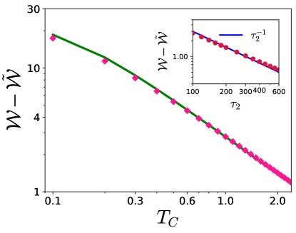
Figure 2: The data points correspond to $\mathcal{W}-\tilde{\mathcal{W}}$ obtained numerically where as the green colored solid line corresponds to the analytical expression obtained by integrating Eq. 18. Clearly, one can observe $1/T_{C}$ scaling at large $T_{C}$. The inset shows $\mathcal{W}-\tilde{\mathcal{W}}$ as a function of $\tau_{2}$ for $T_{C}=1.0$. The blue solid line corresponds to $1/\tau_{2}$. The parameters used are: $L=100,h_{1}=10,h_{2}=1,T_{H}=1000,\tau_{1}=10$.

For TIM, the value of the critical exponents are $\nu=z=1$ which gives

$$\mathcal{W}-\tilde{\mathcal{W}}\sim\frac{1}{T_{C}\tau_{2}}.$$ (32)

One can also obtain the expression for excess defects or excess energy by integrating the analytical expression given in Eq. 18 where $p_{k}$ is given by the Landau Zener probability which in our case takes the form

$$p_{k}=e^{-2\pi\tau_{2}\sin^{2}{k}/(h_{1}-h_{2})}.$$ (33)

We plot in Fig. 2 the numerically obtained $\mathcal{W}-\tilde{\mathcal{W}}$, and compare it with the analytical form given in Eqs. 18 and Eq. 33; as expected, the $1/T_{C}$ scaling given in Eq. 19 is satisfied for large $T_{c}$.

Let us now focus on the work done $\mathcal{|W|}$. We first show the presence of $\tau_{min}$, which is the minimum $\tau$ above which $\mathcal{W}\to\tilde{\mathcal{W}}$. Fig. 3 gives the plot of $\mathcal{|W|}$ as a function of $\tau_{2}$ for different values of $T_{C}$. Clearly, $\mathcal{|W|}$ increases with $\tau_{2}$ till $\tau_{2}\approx\tau_{min}$, after which it saturates. Notably, $\mathcal{|W|}$ saturates at lower $\tau_{2}$ values for higher $T_{C}$, as is predicted by Eq. 25. Further, $|\tilde{\mathcal{W}}|$ is higher for lower $T_{C}$ as expected, and as also seen in Fig. 4. The inset of Fig. 4 shows $\tau_{min}$ as a function of $T_{C}$, where we have taken $\tau_{min}$ as the $\tau_{2}$ value for which $\mathcal{W}-\tilde{\mathcal{W}}<\epsilon$, and compared it with the scaling given by Eq. (25).

In Fig. 5, we plot the maximum output power $|\mathcal{P}(T_{C},\tau_{min})|=|\tilde{W}|/\tau_{min}$ one can obtain without compromising on the work output, i.e., the the output power for $\tau_{2}=\tau_{min}$, which corresponds to approximately the minimum time for which $\mathcal{W}\to\tilde{\mathcal{W}}$, as a function of $T_{C}$. Interestingly, $|\mathcal{P}(T_{C},\tau_{min})|$ increases with increasing $T_{C}$ for small $T_{C}$, attains a maximum at an intermediate value of $T_{C}$, before decreasing with increasing $T_{C}$ for higher $T_{C}$ values. This can be explained as follows: both $\tilde{\mathcal{W}}$ and $\tau_{min}$ decrease with increasing $T_{C}$, which eventually results in a peak in the curve. This suggests the intriguing possibility of an optimum cold bath temperature $T_{C}$ to get high power as well as work output $\mathcal{W}\approx\tilde{\mathcal{W}}$, as opposed to the zero temperature limit where the work output $\mathcal{W}$ will be maximum ($\mathcal{W}\approx\tilde{\mathcal{W}}$) for $\tau_{2}\to\infty$ and $\mathcal{P}(T_{C}\to 0,\tau_{2}\to\infty)\to 0$.

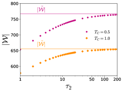
Figure 3: $\mathcal{|W|}$ as a function of $\tau_{2}$ for different values of $T_{C}$. Here the data points correspond to the numerical values and the solid lines correspond to respective $\mathcal{|\tilde{W}|}$ value. The parameters used are : $L=100,h_{1}=10,h_{2}=1,T_{H}=1000,\tau_{1}=10$.

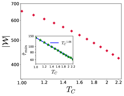
Figure 4: $\mathcal{|W|}$ as a function of $T_{C}$. The parameters used are : $L=100,h_{1}=10,h_{2}=1,T_{H}=1000,\tau_{1}=10,\tau_{2}=100.$ Inset: $\tilde{\tau}_{min}$ as a function of $T_{C}$ where $\tilde{\tau}_{min}$ is the $\tau_{2}$ at which $\mathcal{W}-\tilde{\mathcal{W}}<\epsilon$ where $\epsilon=2$. The fitted blue continuous line corresponds to a slope of $-1.06$, very close to the theoretical value of -1 given by Eq. (25).

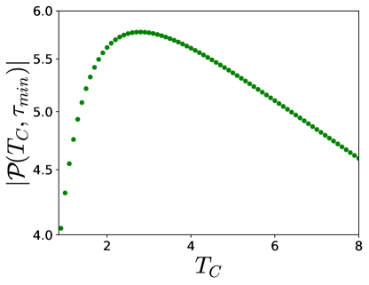
Figure 5: $|\mathcal{P}(T_{C},\tau_{min})|$ as a function of $T_{C}$. Here $|\mathcal{P}(T_{C},\tau_{min})|=\mathcal{|W|}/\tilde{\tau}_{min}$ where $\tilde{\tau}_{min}$ and other parameters are same as in Fig. 4.

6 Conclusion

We construct a many body quantum Otto cycle with a WM that undergoes a quantum phase transition. The non-unitary strokes of the cycle are powered by finite temperature baths, while the unitary strokes involve driving the WM close to the critical point. This driving leads to non-adiabatic excitations which can be quantified using relative excess energy that follows universal scalings with the rate of driving as well as the temperature of the cold bath. The excess energy can be linked to the output work of the engine which thus manifests the universal scalings shown by the excess energy. Notably, we show that higher values of the cold bath temperature $T_{C}$ allows one to operate the engine close to the adiabatic limit for lower values of $\tau_{2}\approx\tau_{min}$, which further follows universal scaling relations. This raises interesting questions regarding the importance of control methods such as shortcuts to adiabaticity [41], or bath engineering [23], for finite temperature quantum heat engines. Furthermore, our results for one-dimensional transverse Ising model WM suggest the existence of an optimal value of the cold bath temperature $T_{C}>0$, for operating the QHE with high work output at high power. These counterintituve results stem from the dominance of thermal fluctuations over quantum fluctuations in finite-temperature quantum critical heat engines, for higher bath temperatures.

Acknowledgements R.B.S. and U.D. acknowledge the use of HPC facility Chandra at IIT Palakkad. U.D. acknowledges support from SERB (SPG/2022/000708). V.M. acknowledges support from SERB through MATRICS (Project No. MTR/2021/000055) and a Seed Grant from IISER Berhampur. Data Availability Statement Any data that support the findings of this study are included within the article.

References

- [1] Jochen Gemmer, Mathias Michel, and Günter Mahler. Quantum thermodynamics: Emergence of thermodynamic behavior within composite quantum systems, volume 784. Springer, 2009.
- [2] Robert Alicki and Ronnie Kosloff. Introduction to Quantum Thermodynamics: History and Prospects. Springer International Publishing, 2018.
- [3] Sai Vinjanampathy and Janet Anders. Quantum thermodynamics. Contemporary Physics, 57:545, 2016.
- [4] Johannes Roßnagel, Samuel T. Dawkins, Karl N. Tolazzi, Obinna Abah, Eric Lutz, Ferdinand Schmidt-Kaler, and Kilian Singer. A single-atom heat engine. Science, 352(6283):325–329, 2016.
- [5] D. von Lindenfels, O. Gräb, C. T. Schmiegelow, V. Kaushal, J. Schulz, Mark T. Mitchison, John Goold, F. Schmidt-Kaler, and U. G. Poschinger. Spin heat engine coupled to a harmonic-oscillator flywheel. Phys. Rev. Lett., 123:080602, Aug 2019.
- [6] John P. S. Peterson, Tiago B. Batalhão, Marcela Herrera, Alexandre M. Souza, Roberto S. Sarthour, Ivan S. Oliveira, and Roberto M. Serra. Experimental characterization of a spin quantum heat engine. Phys. Rev. Lett., 123:240601, Dec 2019.
- [7] James Klatzow, Jonas N. Becker, Patrick M. Ledingham, Christian Weinzetl, Krzysztof T. Kaczmarek, Dylan J. Saunders, Joshua Nunn, Ian A. Walmsley, Raam Uzdin, and Eilon Poem. Experimental demonstration of quantum effects in the operation of microscopic heat engines. Phys. Rev. Lett., 122:110601, Mar 2019.
- [8] Obinna Abah and Eric Lutz. Optimal performance of a quantum otto refrigerator. Europhysics Letters, 113(6):60002, apr 2016.
- [9] Andreas Hartmann, Victor Mukherjee, Glen Bigan Mbeng, Wolfgang Niedenzu, and Wolfgang Lechner. Multi-spin counter-diabatic driving in many-body quantum otto refrigerators. Quantum, 4:377, 2020.
- [10] Thao P. Le, Jesper Levinsen, Kavan Modi, Meera M. Parish, and Felix A. Pollock. Spin-chain model of a many-body quantum battery. Phys. Rev. A, 97:022106, Feb 2018.
- [11] Francesco Campaioli, Felix A. Pollock, and Sai Vinjanampathy. Quantum batteries - review chapter. arXiv: Quantum Physics, 2018.
- [12] Victor Montenegro, Marco G. Genoni, Abolfazl Bayat, and Matteo G. A. Paris. Quantum metrology with boundary time crystals. Communications Physics, 6(1):304, Oct 2023.
- [13] Karl Joulain, Jérémie Drevillon, Younès Ezzahri, and Jose Ordonez-Miranda. Quantum thermal transistor. Phys. Rev. Lett., 116:200601, May 2016.
- [14] Nikhil Gupt, Srijan Bhattacharyya, Bikash Das, Subhadeep Datta, Victor Mukherjee, and Arnab Ghosh. Floquet quantum thermal transistor. Phys. Rev. E, 106:024110, Aug 2022.
- [15] H. T. Quan, Yu-xi Liu, C. P. Sun, and Franco Nori. Quantum thermodynamic cycles and quantum heat engines. Phys. Rev. E, 76:031105, Sep 2007.
- [16] Ronnie Kosloff and Yair Rezek. The quantum harmonic otto cycle. Entropy, 19(4), 2017.
- [17] M. Campisi and R. Fazio. The power of a critical heat engine. Nat. Commun., 7:11895, 2016.
- [18] Thomás Fogarty and Thomas Busch. A many-body heat engine at criticality. Quantum Science and Technology, 6(1):015003, nov 2020.
- [19] Giulia Piccitto, Michele Campisi, and Davide Rossini. The ising critical quantum otto engine. New Journal of Physics, 2022.
- [20] Yu-Han Ma, Shan-He Su, and Chang-Pu Sun. Quantum thermodynamic cycle with quantum phase transition. Phys. Rev. E, 96:022143, Aug 2017.
- [21] Watanabe G. Yu YC Guan XW Chen, YY. and del Campo. An interaction-driven many-particle quantum heat engine and its universal behavior. npj Quantum Inf, 5, 2019.
- [22] Revathy B.S, Victor Mukherjee, Uma Divakaran, and Adolfo del Campo. Universal finite-time thermodynamics of many-body quantum machines from kibble-zurek scaling. Phys. Rev. Res., 2:043247, 2020.
- [23] Revathy B.S, Victor Mukherjee, and Uma Divakaran. Bath engineering enhanced quantum critical engines. Entropy, 24(10), 2022.
- [24] Revathy B.S, Harsh Sharma, and Uma Divakaran. Improving performance of quantum heat engines by free evolution. arXiv preprint arXiv:2302.07003, 2023.
- [25] Jacek Dziarmaga. Dynamics of a quantum phase transition: Exact solution of the quantum ising model. Phys. Rev. Lett., 95:245701, Dec 2005.
- [26] Victor Mukherjee, Uma Divakaran, Amit Dutta, and Diptiman Sen. Quenching dynamics of a quantum spin- chain in a transverse field. Phys. Rev. B, 76:174303, Nov 2007.
- [27] K. Sengupta, Diptiman Sen, and Shreyoshi Mondal. Exact results for quench dynamics and defect production in a two-dimensional model. Phys. Rev. Lett., 100:077204, Feb 2008.
- [28] Maximilian Keck, Simone Montangero, Giuseppe E Santoro, Rosario Fazio, and Davide Rossini. Dissipation in adiabatic quantum computers: lessons from an exactly solvable model. New Journal of Physics, 19(11):113029, nov 2017.
- [29] Souvik Bandyopadhyay, Sudarshana Laha, Utso Bhattacharya, and Amit Dutta. Exploring the possibilities of dynamical quantum phase transitions in the presence of a markovian bath. Scientific Reports, 8(1):11921, 2018.
- [30] Bogdan Damski and Wojciech H. Zurek. Adiabatic-impulse approximation for avoided level crossings: From phase-transition dynamics to landau-zener evolutions and back again. Phys. Rev. A, 73:063405, Jun 2006.
- [31] Anatoli Polkovnikov, Krishnendu Sengupta, Alessandro Silva, and Mukund Vengalattore. Colloquium: Nonequilibrium dynamics of closed interacting quantum systems. Rev. Mod. Phys., 83:863–883, Aug 2011.
- [32] Adolfo Del Campo and Wojciech H Zurek. Universality of phase transition dynamics: Topological defects from symmetry breaking. International Journal of Modern Physics A, 29(08):1430018, 2014.
- [33] Amit Dutta, Gabriel Aeppli, Bikas K Chakrabarti, Uma Divakaran, Thomas F Rosenbaum, and Diptiman Sen. Quantum phase transitions in transverse field spin models: from statistical physics to quantum information. Cambridge University Press, 2015.
- [34] A. Polkovnikov and V. Gritsev. Breakdown of the adiabatic limit in low-dimensional gapless systems. Nature Physics, 4:477, June 2008.
- [35] C. De Grandi, V. Gritsev, and A. Polkovnikov. Quench dynamics near a quantum critical point: Application to the sine-gordon model. Phys. Rev. B, 81:224301, Jun 2010.
- [36] C. De Grandi, V. Gritsev, and A. Polkovnikov. Quench dynamics near a quantum critical point. Phys. Rev. B, 81:012303, Jan 2010.
- [37] Shusa Deng, Gerardo Ortiz, and Lorenza Viola. Dynamical critical scaling and effective thermalization in quantum quenches: Role of the initial state. Phys. Rev. B, 83:094304, 2011.
- [38] Pierre Pfeuty. The one-dimensional ising model with a transverse field. Annals of Physics, 57(1):79 – 90, 1970.
- [39] J. E. Bunder and Ross H. McKenzie. Effect of disorder on quantum phase transitions in anisotropic xy spin chains in a transverse field. Phys. Rev. B, 60:344–358, Jul 1999.
- [40] Elliott Lieb, Theodore Schultz, and Daniel Mattis. Two soluble models of an antiferromagnetic chain. Annals of Physics, 16(3):407 – 466, 1961.
- [41] Andreas Hartmann, Victor Mukherjee, Wolfgang Niedenzu, and Wolfgang Lechner. Many-body quantum heat engines with shortcuts to adiabaticity. Phys. Rev. Res., 2:023145, May 2020.