Risk exchange under infinite-mean Pareto models

Abstract

We study the optimal decisions and equilibria of agents who aim to minimize their risks by allocating their positions over extremely heavy-tailed (i.e., infinite-mean) and possibly dependent losses. The loss distributions of our focus are super-Pareto distributions, which include the class of extremely heavy-tailed Pareto distributions. Using a recent result on stochastic dominance, we show that for a portfolio of super-Pareto losses, non-diversification is preferred by decision makers equipped with well-defined and monotone risk measures. The phenomenon that diversification is not beneficial in the presence of super-Pareto losses is further illustrated by an equilibrium analysis in a risk exchange market. First, agents with super-Pareto losses will not share risks in a market equilibrium. Second, transferring losses from agents bearing super-Pareto losses to external parties without any losses may arrive at an equilibrium which benefits every party involved.

Keywords: super-Pareto distributions; diversification; risk exchange; equilibrium; risk measures.

1 Introduction

Over the last decades, the insurance industry has observed a rising trend in both the frequency and magnitude of huge losses caused by natural disasters and man-made catastrophes (e.g., Embrechts et al., (1999)). In quantitative risk management, Pareto distributions (or generalized Pareto distributions) have been widely used in modeling catastrophic losses (see McNeil et al., (2015)), mainly due to their unique role in Extreme Value Theory (EVT): By the Pickands-Balkema-de Haan Theorem (Pickands, (1975) and Balkema and de Haan, (1974)), generalized Pareto distributions are the only possible non-degenerate limiting distributions of excess-of-loss random variables. Although statistical and actuarial methods often focus on finite-mean EVT models, data analyses in the literature show that the best-fitted models for many catastrophic losses in various contexts do not have finite means. At the end of this section, we collect many examples and related literature on infinite-mean Pareto-type models.

It is well known that infinite-mean models lead to intriguing phenomenon in risk management; see e.g., Ibragimov et al. (2011). This paper focuses on the following question.

1. Suppose that there is a pool of identically distributed extremely heavy-tailed losses (i.e., infinite mean), possibly statistically dependent. Each agent (e.g., a reinsurance provider) needs to decide whether and how to diversify in this pool. Without knowing the preferences of the agents, what can we say about the optimal decisions and equilibria in a multiple-agent setting?

Assume for simplicity that the losses in the pool, denoted by $X_{1},\dots,X_{n}$, are independent and identically distributed (iid) Pareto losses with infinite mean. Let $\theta_{1},\dots,\theta_{n}\geq 0$ with $\sum_{i=1}^{n}\theta_{i}=1$ be the exposures of an agent over $X_{1},\dots,X_{n}$. Our analysis is built on a recent result of Chen et al. (2024) that gives

$$X_{1}\leq_{\rm st}\theta_{1}X_{1}+\dots+\theta_{n}X_{n},$$ (1)

where $\leq_{\rm st}$ stands for first-order stochastic dominance; that is, for two random variables $X$ and $Y$, $X\leq_{\rm st}Y$ if $\mathbb{P}(X\leq x)\geq\mathbb{P}(Y\leq x)$ for all $x\in\mathbb{R}$. This inequality is shown to be strict when the agent holds at least two losses in their portfolio. Intuitively, the left-hand side of (1) is a portfolio concentrated on $X_{1}$, and the right-hand side is a diversified portfolio of $X_{1},\dots,X_{n}$. Inequality (1) implies that if the agent aims to minimize their default probability, the optimal decision is non-diversification; this observation is generalized in Section 4.

Besides iid Pareto losses with infinite mean, (1) and its implications also hold for weakly negatively associated and identically distributed super-Pareto losses by Theorem 1 of Chen et al. (2024); we briefly summarize in Section 2 the definitions of super-Pareto distributions and weak negative association. Section 3 presents several generalizations of (1) beyond weakly negatively associated super-Pareto models considered by Chen et al. (2024). Propositions 1 and 2 provide some high-level conditions for generalizing the marginal distributions and the dependence structure. Proposition 3 provides a model for losses that are super-Pareto only in the tail region and Proposition 4 considers a classic insurance model.

We discuss in Section 4 useful decision models in the presence of extremely heavy-tailed losses and the implications of (1) and related inequalities on the risk management decision of a single agent. First, although (1) never holds for non-degenerate random variables with finite mean (see Proposition 2 in Chen et al. (2024)), we show that a similar preference for non-diversification exists for truncated super-Pareto losses, as long as the thresholds are high enough (Theorem 2). Second, for super-Pareto losses, the action of diversification increases the risk uniformly for all risk preferences, such as VaR, expected utilities, and distortion risk measures, as long as the risk preferences are monotone and well-defined. The increase of the portfolio risk is strict, and it provides an important implication in decision making: For an agent who faces super-Pareto losses and aims to minimize their risk by choosing a position across these losses, the optimal decision is to take only one of the super-Pareto losses (i.e., no diversification).

We proceed to study the equilibria of a risk exchange market for super-Pareto losses in Section 5. As individual agents do not benefit from diversification over super-Pareto losses, we may expect that agents will not share their losses. Indeed, if each agent in the market is associated with an initial position in one super-Pareto loss, the agents will merely exchange the entire loss position instead of risk sharing in an equilibrium model (Theorem 3 (i)). The situation becomes quite different if the agents with initial losses can transfer their losses to external parties. If the external agents have a stronger risk tolerance than the internal agents, both parties may benefit by transferring losses from the internal to the external agents (Theorem 4 (ii)). In Proposition 7, we show that agents prefer to share losses with finite mean among themselves; this is in sharp contrast to the case of super-Pareto losses.

In Section 6, some examples are presented to illustrate the presence of extremely heavy tails in two real datasets in which the phenomenon of inequality (1) or its generalizations can be empirically observed. Section 7 concludes the paper. Some background on risk measures is put in Appendix A. Proofs of all results are put in Appendix B.

Review of infinite-mean Pareto-type models. The key assumption of our paper is that losses follow super-Pareto distributions, which have infinite mean. Whereas statistical models with some divergent higher moments are ubiquitous throughout the risk management literature, the infinite mean case needs more specific motivation. For power-tail data, a standard approach for the estimation of the underlying tail parameters is the Peaks Over Threshold (POT) methodology from EVT; see Embrechts et al. (1997). Other estimation methods include the classic Hill estimators (see Embrechts et al. (1997)) and the log-log rank-size estimation (see Ibragimov et al., (2015)). It is known that the Hill estimator may be sensitive to the dependence in the data and small sample sizes, and the log-log rank-size estimation can be biased in small samples; see Gabaix and Ibragimov, (2011) for an improved version of log-log rank-size estimation. Below we discuss some examples from the literature leading to extremely heavy-tailed Pareto models.

In the parameterization used in Section 2, a tail parameter $\alpha\leq 1$ corresponds to an infinite-mean Pareto model. Ibragimov et al. (2009) used standard seismic theory to show that the tail indices $\alpha$ of earthquake losses lie in the range $[0.6,1.5]$. Estimated by Rizzo, (2009), the tail indices $\alpha$ for some wind catastrophic losses are around $0.7$. Hofert and Wüthrich, (2012) showed that the tail indices $\alpha$ of losses caused by nuclear power accidents are around $[0.6,0.7]$; similar observations can be found in Sornette et al., (2013). Based on data collected by the Basel Committee on Banking Supervision, Moscadelli, (2004) reported the tail indices $\alpha$ of (over $40000$) operational losses in $8$ different business lines to lie in the range $[0.7,1.2]$, with $6$ out of the $8$ tail indices being less than $1$, with $2$ out of these $6$ significantly less than $1$ at a $95\%$ confidence level. For a detailed discussion on the risk management consequences in this case, see Nešlehová et al., (2006). Losses from cyber risk have tail indices $\alpha\in[0.6,0.7]$; see Eling and Wirfs, (2019), Eling and Schnell, (2020) and the references therein. In a standard Swiss Solvency Test document (FINMA, (2021, p. 110)), most major damage insurance losses are modelled by a Pareto distribution with default parameter $\alpha$ in the range $[1,2]$, with $\alpha=1$ attained by some aircraft insurance. As discussed by Beirlant et al., (1999), some fire losses collected by the reinsurance broker AON Re Belgium have tail indices $\alpha$ around $1$. Biffis and Chavez, (2014) showed that several large commercial property losses collected from two Lloyd’s syndicates have tail indices $\alpha$ considerably less than $1$. Silverberg and Verspagen, (2007) concluded that the tail indices $\alpha$ are less than $1$ for financial returns from some technological innovations. The tail part of cost overruns in information technology projects can have tail indices $\alpha\leq 1$; see Flyvbjerg et al., (2022). In the model of Cheynel et al., (2024), which considers managers’ fraudulent behavior, detected fraud size behaves like a power law with tail index 1. Besides large financial losses and returns, the number of deaths in major earthquakes and pandemics modelled by Pareto distributions also has infinite mean; see Clark, (2013) and Cirillo and Taleb, (2020). City sizes and firm sizes follow Zipf’s law ($\alpha\approx 1$); see Gabaix, (1999) and Axtell, (2001). Heavy-tailed to extremely heavy-tailed models also occur in the realm of climate change and environmental economics. Weitzman’s Dismal Theorem (see Weitzman (2009)) discusses the breakdown of standard economic thinking like cost-benefit analysis in this context. This led to an interesting discussion with William Nordhaus, a recipient of the 2018 Nobel Memorial Prize in Economic Sciences; see Nordhaus, (2009).

The above references exemplify the occurrence of infinite mean models. Our perspective on these examples and discussions is that if these models are the result of some careful statistical analyses, then the practicing modeler has to take a step back and carefully reconsider the risk management consequences. Of course, in practice, there are several methods available to avoid such extremely heavy-tailed models, like cutting off the loss distribution model at some specific level or tapering (concatenating a light-tailed distribution far in the tail of the loss distribution). In examples like those referred to above, such corrections often come at the cost of a great variability depending on the methodology used. It is in this context that our results add to the existing literature and modeling practice in cases where power-tail data play an important role.

2 Preliminaries

Throughout, random variables are defined on an atomless probability space $(\Omega,\mathcal{F},\mathbb{P})$. Denote by $\mathbb{N}$ the set of all positive integers and $\mathbb{R}_{+}$ the set of non-negative real numbers. For $n\in\mathbb{N}$, let $[n]=\{1,\dots,n\}$. Denote by $\Delta_{n}$ the standard simplex, that is, $\Delta_{n}=\{(\theta_{1},\dots,\theta_{n})\in[0,1]^{n}:\sum_{i=1}^{n}\theta_{i}=1\}$. For $x,y\in\mathbb{R}$, write $x\wedge y=\min\{x,y\}$ and $x_{+}=\max\{x,0\}$. We write $\mathbf{X}\buildrel\mathrm{d}\over{=}\mathbf{Y}$ if $\mathbf{X}$ and $\mathbf{Y}$ have the same distribution. We always assume $n\geq 2$. Equalities and inequalities are interpreted component-wise when applied to vectors. For any random variable $X$, its essential infimum is given by $z_{X}=\inf\{z\in\mathbb{R}:\mathbb{P}(X>z)>0\}$, and its distribution function is denoted by $F_{X}$. In this paper, all terms like “increasing” and “decreasing” are in the non-strict sense.

We first introduce the super-Pareto distribution and weak negative association, and present the main result of Chen et al. (2024), on which most of our study is based. The distribution function of a Pareto random variable with parameters $\theta,\alpha>0$ is

$$P_{\alpha,\theta}(x)=1-\left(\frac{\theta}{x}\right)^{\alpha},~{}~{}x\geq\theta.$$

The mean of $P_{\alpha,\theta}$ is infinite (i.e., $P_{\alpha,\theta}$ is extremely heavy-tailed) if and only if the tail parameter $\alpha\in(0,1]$. As it suffices to consider $P_{\alpha,1}$ in this paper, we write $P_{\alpha,1}$ as $\mathrm{Pareto}(\alpha)$.

Definition 1.

A random variable $X$ is super-Pareto (or has a super-Pareto distribution) if $X\buildrel\mathrm{d}\over{=}f(Y)$ for some increasing, convex, and non-constant function $f$ and $Y\sim\mathrm{Pareto}(1)$.

As super-Pareto losses can be obtained by increasing and convex transforms of Pareto($1$) losses, their tails are heavier than (or equivalent to) those of Pareto($1$) losses and thus have infinite mean. All extremely heavy-tailed Pareto distributions are super-Pareto. Other examples of super-Pareto distributions include special cases of generalized Pareto distributions, Burr distributions, paralogistic distributions, and log-logistic distributions; see Chen et al. (2024).

Definition 2.

A set $S\subseteq\mathbb{R}^{k}$, $k\in\mathbb{N}$, is decreasing if $\mathbf{x}\in S$ implies $\mathbf{y}\in S$ for all $\mathbf{y}\leq\mathbf{x}$. Random variables $X_{1},\dots,X_{n}$ are weakly negatively associated if for any $i\in[n]$, decreasing set $S\subseteq\mathbb{R}^{n-1}$, and $x\in\mathbb{R}$ with $\mathbb{P}(X_{i}\leq x)>0$, it holds that $\mathbb{P}(\mathbf{X}_{-i}\in S\mid X_{i}\leq x)\leq\mathbb{P}(\mathbf{X}_{-i}\in S),$ where $\mathbf{X}_{-i}=(X_{1},\dots,X_{i-1},X_{i+1},\dots,X_{n})$.

Weak negative association includes independence as a special case. Weak negative association is implied by negative association (Alam and Saxena (1981) and Joag-Dev and Proschan (1983)) and negative regression dependence (Lehmann (1966) and Block et al., (1985)), and it implies negative orthant dependence (Block et al., (1982)). Multivaraite normal distributions with non-positive correlations are negatively associated and thus are weakly negatively associated.

This paper mainly considers weakly negatively associated and identically distributed (WNAID) super-Pareto random variables. This setting includes iid Pareto losses with infinite mean. For random variables $X$ and $Y$, we write $X<_{\rm st}Y$ if $\mathbb{P}(X>x)<\mathbb{P}(Y>x)$ for all $x\in\mathbb{R}$ satisfying $\mathbb{P}(X>x)\in(0,1)$, and this will be referred to as strict stochastic dominance. The following result serves as the basis for our study.

Theorem 1 (Chen et al. (2024)).

Let $X_{1},\dots,X_{n}$ be WNAID super-Pareto and $X\buildrel\mathrm{d}\over{=}X_{1}$. For $(\theta_{1},\dots,\theta_{n})\in\Delta_{n}$, we have

$$X\leq_{\rm st}\sum_{i=1}^{n}\theta_{i}X_{i}.$$ (2)

Moreover, strict stochastic dominance $X<_{\rm st}\sum_{i=1}^{n}\theta_{i}X_{i}$ holds if $\theta_{i}>0$ for at least two $i\in[n]$.

Inequality (2) implies that for an agent who wants to minimize the default probability of their loss portfolio, the optimal strategy is non-diversification. A similar inequality to (2) also holds in a model for catastrophic losses (i.e., a loss can be written as $Y\mathds{1}_{A}$ where $Y$ is a loss given the occurrence of a catastrophic event $A$), obtained in Theorem 1 (ii) of Chen et al. (2024), which we omit. Other generalizations of (2) will be obtained in Section 3.

3 Generalizations of the super-Pareto stochastic dominance

We discuss whether and how (2) can be generalized beyond the WNAID super-Pareto model. That is, whether

$$X\leq_{\rm st}\sum_{i=1}^{n}\theta_{i}X_{i}~{}\mbox{for all $(\theta_{1},\dots,\theta_{n})\in\Delta_{n}$, where $X,X_{1},\dots,X_{n}$ are identically distributed}$$ (DP)

holds under models other than those covered in Theorem 1 (“DP” stands for “diversification penalty”). We consider two directions of generalizations, one on the marginal distributions and one on the dependence structure. Below, $n\geq 2$ is fixed. First, let

$$\mathcal{F}_{\mathrm{IN}}=\{\mbox{distribution of $X$}:\mbox{\eqref{eq:R2-new} holds for all independent $X_{1},\dots,X_{n}$}\}.$$

The set $\mathcal{F}_{\mathrm{WNA}}$ is defined similarly, where the subscript WNA means weak negative association instead of independence, among $X_{1},\dots,X_{n}$. Clearly, $\mathcal{F}_{\mathrm{WNA}}\subseteq\mathcal{F}_{\mathrm{IN}}$, and each of them contains all super-Pareto distributions by Theorem 1. Below, by considering transforms on $\mathcal{F}_{\mathrm{WNA}}$ and $\mathcal{F}_{\mathrm{IN}}$, we mean that the transform is applied to the random variable $X$.

Proposition 1.

The set $\mathcal{F}_{\mathrm{IN}}$ is closed under convolution. Both $\mathcal{F}_{\mathrm{WNA}}$ and $\mathcal{F}_{\mathrm{IN}}$ are closed under strictly increasing convex transforms.

The second statement in Proposition 1 means (DP) also holds for strictly increasing convex transforms of $X,X_{1},\dots,X_{n}$ given some dependence assumptions (i.e., $f(X)\leq_{\rm st}\sum_{i=1}^{n}\theta_{i}f(X_{i})$ where $f$ is any strictly increasing convex function).

Second, we consider possible dependence structures for (DP). Copulas are useful tools for modeling dependence structures; see Nelsen (2006) for an overview. A copula is a distribution function with standard uniform (i.e., on $[0,1]$) marginal distributions. For a random vector $\mathbf{X}$ with distribution function $F$ and marginal distributions $F_{1},\dots,F_{n}$, by Sklar’s Theorem (e.g., Theorem 7.3 of McNeil et al., (2015)), there exists a copula $C$ satisfying $F(x_{1},\dots,x_{n})=C(F_{1}(x_{1}),\dots,F_{n}(x_{n}))$ for $(x_{1},\dots,x_{n})\in\mathbb{R}^{n}$, and such $C$ is called a copula of $\mathbf{X}$, which is unique when $\mathbf{X}$ has continuous marginal distributions. The copula for independence and the copula for comonotonicity are given by $\mathbf{u}\mapsto\prod_{i=1}^{n}u_{i}$ and $\mathbf{u}\mapsto\min(\mathbf{u})$ for $\mathbf{u}=(u_{1},\dots,u_{n})\in[0,1]^{n}$, respectively. A copula for weak negative association is any copula of weakly negatively associated standard uniform random variables. As their names suggest, these copulas represent the corresponding dependence structures. The set of dependence structures satisfying (DP) is then represented by

$$\mathcal{C}_{\mathrm{DP}}=\{\mbox{copula }C:\mbox{\eqref{eq:R2-new} holds for all super-Pareto $X_{1},\dots,X_{n}$ with copula $C$}\}.$$

Proposition 2.

The set $\mathcal{C}_{\mathrm{DP}}$ is closed under mixture, and it contains all copulas for comonotonicity, independence, and weak negative association.

By Proposition 2, (DP) holds under some particular forms of positive or mixed dependence, in addition to the weak negative association studied by Chen et al. (2024). Nevertheless, we did not find a natural model of positive dependence, other than a mixture of independence and comonotonicity, that yields (DP).

We present below two additional models for which similar results to Theorem 1 hold: the tail super-Pareto distribution model, and the collective risk model in insurance.

As reflected by the Pickands-Balkema-de Haan Theorem (see Theorem 3.4.13 (b) of Embrechts et al. (1997)), many losses have a power-like tail, but their distributions may not be power-like over the full support. Therefore, it is practically useful to assume that a random loss has a Pareto distribution only in the tail region; see the examples in the Introduction.

Let $X$ be a super-Pareto random variable. We say that $Y$ is distributed as $X$ beyond $x$ if $\mathbb{P}(Y>t)=\mathbb{P}(X>t)$ for $t\geq x$. Our next result suggests that, under an extra condition, a stochastic dominance also holds in the tail region for such distributions.

Proposition 3.

Let $X$ be a super-Pareto random variable, $Y_{1},\dots,Y_{n}$ be iid random variables distributed as $X$ beyond $x\geq z_{X}$, and $Y\buildrel\mathrm{d}\over{=}Y_{1}$. Assume that $Y\geq_{\rm st}X$. For $(\theta_{1},\dots,\theta_{n})\in\Delta_{n}$ and $t\geq x$, we have $\mathbb{P}\left(\sum_{i=1}^{n}\theta_{i}Y_{i}>t\right)\geq\mathbb{P}\left(Y>t\right)$, and the inequality is strict if $t>z_{X}$ and $\theta_{i}>0$ for at least two $i\in[n]$.

In Proposition 3, the assumption $Y\geq_{\rm st}X$, that is, $\mathbb{P}(Y>t)\geq\mathbb{P}(X>t)$ for $t\in[z_{X},x]$, is not dispensable. Here we cannot allow the distribution of $Y$ on $[z_{X},x]$ to be arbitrary; the entire distribution is relevant to establish the inequality $\mathbb{P}\left(\sum_{i=1}^{n}\theta_{i}Y_{i}>t\right)\geq\mathbb{P}\left(Y>t\right)$, even for $t$ in the tail region.

Random weights and a random number of risks are, for instance, common in modeling portfolios of insurance losses; see Klugman et al. (2012). Let $N$ be a counting random variable (i.e., it takes values in $\{0,1,2,\dots\}$), and $W_{i}$ and $X_{i}$ be positive random variables for $i\in\mathbb{N}$. We consider an insurance portfolio where each policy incurs a loss $W_{i}X_{i}$ if there is a claim, and $N$ is the total number of claims in a given period. If $W_{1}=W_{2}=\dots=1$ and $X_{1},X_{2},\dots$ are iid, then this model recovers the classic collective risk model. The portfolio loss of insurance policies is given by ${\sum_{i=1}^{N}W_{i}X_{i}},$ and its average loss across claims is $({\sum_{i=1}^{N}W_{i}X_{i}})/({\sum_{i=1}^{N}W_{i}})$ where both terms are $0$ if $N=0$.

Proposition 4.

Let $X_{1},X_{2},\dots$ be WNAID super-Pareto random variables, $X\buildrel\mathrm{d}\over{=}X_{1}$, $W_{1},W_{2},\dots$ be positive random variables, and $N$ be a counting random variable, such that $X,\{X_{i}\}_{i\in\mathbb{N}}$, $\{W_{i}\}_{i\in\mathbb{N}}$, and $N$ are independent. We have

$$X\mathds{1}_{\{N\geq 1\}}\leq_{\rm st}\frac{\sum_{i=1}^{N}W_{i}X_{i}}{\sum_{i=1}^{N}W_{i}}\mbox{~{}~{}~{}and~{}~{}~{}}\sum_{i=1}^{N}W_{i}X\leq_{\rm st}{\sum_{i=1}^{N}W_{i}X_{i}}.$$ (3)

If $\mathbb{P}(N\geq 2)\neq 0$, then for $t>z_{X}$, $\mathbb{P}(\sum_{i=1}^{N}W_{i}X_{i}/\sum_{i=1}^{N}W_{i}\leq t)<\mathbb{P}(X\mathds{1}_{\{N\geq 1\}}\leq t)$.

If $W_{1}=W_{2}=\dots=1$ as in the classic collective risk model, then, under the assumptions of Proposition 4, we have

$$X_{1}\mathds{1}_{\{N\geq 1\}}\leq_{\rm st}\frac{1}{N}{\sum_{i=1}^{N}X_{i}}\mbox{~{}~{}~{}and~{}~{}~{}}NX_{1}\leq_{\rm st}{\sum_{i=1}^{N}X_{i}}.$$

The above inequalities suggest that the sum of a randomly counted sequence of WNAID super-Pareto losses is stochastically larger than the sum of a randomly counted sequence of identical super-Pareto losses. Therefore, building an insurance portfolio for WNAID super-Pareto claims does not reduce the total risk. In this setting, it is less risky to insure identical policies than to insure weakly negatively associated policies of the same type of super-Pareto loss and thus the basic principle of insurance does not apply to super-Pareto losses.

4 Risk management implications

4.1 Decision models for infinite-mean risks

The interpretation of Theorem 1 and its several generalizations in Section 3 is that non-diversification is better than diversification in a pool of extremely heavy-tailed losses. We first discuss useful decision models for which this result can or cannot be applied.

Denote by $\mathcal{X}$ the set of all random variables and $L^{1}\subseteq\mathcal{X}$ the set of random variables with finite mean. Assume that $X_{1},\dots,X_{n}$ are WNAID super-Pareto and $(\theta_{1},\dots,\theta_{n})\in\Delta_{n}$ with at least two of $\theta_{1},\dots,\theta_{n}$ being positive. Let $\mathcal{L}\subseteq\mathcal{X}$ be a set of random variables representing possible losses to an agent, such that $\sum_{i=1}^{n}\theta_{i}X_{i}\in\mathcal{L}$ and $X_{1}\in\mathcal{L}$. Moreover, assume that $\mathcal{L}$ is law invariant; that is, $X\in\mathcal{L}$ and $X\buildrel\mathrm{d}\over{=}Y$ imply $Y\in\mathcal{L}$.

The preferences of the agent are represented by a transitive binary relation $\succeq$ (with strict relation $\succ$ and symmetric relation $\simeq$) on $\mathcal{L}$, which we assume to satisfy two natural properties:

1. Choice under risk: $X\simeq Y$ for $X,Y\in\mathcal{L}$ if $X\buildrel\mathrm{d}\over{=}Y$;

2. Less loss is better: $X\succeq Y$ for $X,Y\in\mathcal{L}$ if $X\leq Y$ (in the almost sure sense, omitted below).

By Theorem 1 and the representation of first-order stochastic dominance (see e.g., Shaked and Shanthikumar, (2007, Theorem 1.A.1)),

$$X_{1}\leq_{\rm st}\sum_{i=1}^{n}\theta_{i}X_{i}\implies\mbox{there exists $Y\buildrel\mathrm{d}\over{=}X_{1}$ such that }Y\leq\sum_{i=1}^{n}\theta_{i}X_{i}\implies X_{1}\simeq Y\succeq\sum_{i=1}^{n}\theta_{i}X_{i}.$$

A standard construction of $Y$ is to let $Y=h(U)$, where $U$ is uniformly distributed on $[0,1]$ such that $\sum_{i=1}^{n}\theta_{i}X_{i}=g(U)$, and $g$ and $h$ are the left quantile functions of $\sum_{i=1}^{n}\theta_{i}X_{i}$ and $X_{1}$, respectively. Therefore, any agent satisfying (i) and (ii) would (weakly) prefer non-diversification modelled by $X_{1}$ to diversification modelled by $\sum_{i=1}^{n}\theta_{i}X_{i}$. Moreover, we can further consider

1. Less loss is strictly better: $X\succ Y$ for $X,Y\in\mathcal{L}$ if $\mathbb{P}(X<Y)=1$.

If (iii) holds, then we have a strict preference $X_{1}\succ\sum_{i=1}^{n}\theta_{i}X_{i},$ following the argument above.

Risk measures are an important tool to evaluate portfolio risks for financial institutions and many of them induce the binary relation discussed above. A risk measure is a functional $\rho:\mathcal{X}_{\rho}\rightarrow\overline{\mathbb{R}}:=[-\infty,\infty]$, where the domain $\mathcal{X}_{\rho}\subseteq\mathcal{X}$ is a set of random variables representing financial losses. We will assume that an agent uses a risk measure $\rho$ for their preference, in the sense that $\rho(X)\leq\rho(Y)\Leftrightarrow X\succeq Y$. Our notion of a risk measure is quite broad, and it includes not only risk measures in the sense of Artzner et al. (1999) and Föllmer and Schied (2016) but also decision models such as the expected utility by flipping the sign. The assumptions on $\rho$ below correspond to (i), (ii) and (iii) respectively.

1. Law invariance: $\rho(X)=\rho(Y)$ for $X,Y\in\mathcal{X}_{\rho}$ if $X\buildrel\mathrm{d}\over{=}Y$.

2. Weak monotonicity: $\rho(X)\leq\rho(Y)$ for $X,Y\in\mathcal{X}_{\rho}$ if $X\leq_{\rm st}Y$.

3. Mild monotonicity: $\rho$ is weakly monotone and $\rho(X)<\rho(Y)$ for $X,Y\in\mathcal{X}_{\rho}$ if $\mathbb{P}(X<Y)=1$.

Many commonly used decision models are not just weakly monotone but mildly monotone; we highlight some examples. First, for an increasing utility function $u$, the expected utility agent can be represented by a risk measure $E_{v}$, namely

$$E_{v}(X)=\mathbb{E}[v(X)],~{}~{}~{}~{}~{}~{}X\in\mathcal{X}_{E_{v}}:=\{Y\in\mathcal{X}:\mathbb{E}[|v(Y)|]<\infty\},$$

where $v(x)=-u(-x)$ is also increasing. It is clear that $E_{v}$ is mildly monotone if $v$ or $u$ is strictly increasing. Note that for risk-averse expected utility decision makers ($u$ is concave), the domain of $E_{v}$ is typically smaller than $\mathcal{L}$. However, there are still a few useful contexts where expected utility models can be used to compare infinite-mean losses. Below we give a few examples.

1. Suppose that for some $\ell\in\mathbb{R}$, $u(x)=u(\ell)$ for all $x\leq\ell$, and $u$ is concave on $(\ell,\infty)$. This utility function describes a risk-averse agent with limited liability. Limited liability is a practical assumption in banking and insurance decisions for both individuals and financial institutions.

2. The Markowitz utility function (Markowitz (1952)) has a convex-concave structure on the loss side, which is based on the empirical observation that people often prefer a loss of $10m$ dollars with $0.1$ probability over a sure loss of $m$ dollars when $m$ is very large.

3. In the cumulative prospect theory (which generalizes the expected utility model) of Tversky and Kahneman (1992), the utility function is convex below a reference point.

In all cases above, the expected utility can take finite values on $\mathcal{L}$ and is mildly monotone, implying a strict preference for non-diversification.

The next examples of mildly monotone risk measures are the two widely used regulatory risk measures in insurance and finance, Value-at-Risk (VaR) and Expected Shortfall (ES). For $X\in\mathcal{X}$ and $p\in(0,1)$, VaR is defined as

$$\mathrm{VaR}_{p}(X)=F^{-1}_{X}(p)=\inf\{t\in\mathbb{R}:F_{X}(t)\geq p\},$$

and ES is defined as

$$\mathrm{ES}_{p}(X)=\frac{1}{1-p}\int_{p}^{1}\mathrm{VaR}_{u}(X)\mathrm{d}u.$$

For $X\notin L^{1}$, such as super-Pareto losses, $\mathrm{ES}_{p}(X)$ can be $\infty$, whereas $\mathrm{VaR}_{p}(X)$ is always finite. Therefore, VaR is mildly monotone on $\mathcal{X}$, whereas ES is mildly monotone only on $L^{1}$. Note that convex risk measures will take infinite values when evaluating infinite-mean losses and hence are not suitable for losses in $\mathcal{L}$; standard properties of risk measures are collected in Appendix A.

4.2 Diversification penalty for losses with bounded support

Although (2) never holds for non-degenerate random variables with finite mean (Proposition 2 in Chen et al. (2024)), Theorem 1 can be applied to some contexts of finite-mean losses. Since (strict) first-order stochastic dominance is preserved under (strictly) increasing transformations, Theorem 1 implies $h(X_{1})\leq_{\rm st}h(\sum_{i=1}^{n}\theta_{i}X_{i})$ for all increasing real functions $h$. For instance, in the context of reinsurance, $h(x)=x\wedge c$ for some threshold $c\in\mathbb{R}$ corresponds to an excess-of-loss reinsurance coverage; see e.g., OECD (2018). On the other hand, for an increasing transform $h$ performed on individual losses, the first-order stochastic dominance $h(X_{1})\leq_{\rm st}\sum_{i=1}^{n}\theta_{i}h(X_{i})$ may not hold, unless $h$ is convex (see Lemma 2 in Chen et al. (2024)). Especially, if $\mathbb{E}[h(X_{1})]<\infty$ (this cannot happen if $h$ is convex and non-constant) and $X_{1},\dots,X_{n}$ are iid, then $h(X_{1})\geq_{\rm cx}\sum_{i=1}^{n}\theta_{i}h(X_{i})$ holds, where $Y\geq_{\rm cx}Z$ means $\mathbb{E}[\phi(Y)]\geq\mathbb{E}[\phi(Z)]$ for all convex $\phi$ such that the expectations exist. With finite mean, a risk-averse expected utility agent would favour diversification, a well-known phenomenon; see, e.g., Samuelson, (1967). Although $g(X_{1})\leq_{\rm st}\sum_{i=1}^{n}\theta_{i}g(X_{i})$ fails to hold in case $g$ is bounded, non-diversification is still preferred for $\mathrm{VaR}_{p}$ with specific $p$ when $g(x)=x\wedge c$. We present a generalization, allowing a different threshold for each loss, in the following result.

Theorem 2.

Let $X,X_{1},\dots,X_{n}$ be WNAID super-Pareto random variables and $Y_{i}=X_{i}\wedge c_{i}$ where $c_{i}\geq z_{X}$ for each $i\in[n]$. Suppose that $(\theta_{1},\dots,\theta_{n})\in\Delta_{n}$ such that $\theta_{i}>0$ for at least two $i\in[n]$, and denote by $c=\min\{c_{1}\theta_{1},\dots,c_{n}\theta_{n}\}$. We have

$$\mathbb{P}\left(\sum_{i=1}^{n}\theta_{i}Y_{i}>t\right)=\mathbb{P}\left(\sum_{i=1}^{n}\theta_{i}X_{i}>t\right)>\mathbb{P}\left(X>t\right)=\mathbb{P}\left(Y_{i}>t\right),~{}~{}~{}i\in[n]$$

for $t\in(z_{X},c]$, and

$$\mathrm{VaR}_{p}\left(\sum_{i=1}^{n}\theta_{i}Y_{i}\right)>\sum_{i=1}^{n}\theta_{i}\mathrm{VaR}_{p}(Y_{i})$$

for $p\in(0,\mathbb{P}(X\leq c))$.

Theorem 2 states that for a fixed weight vector of positive components and a fixed $p\in(0,1)$, if the thresholds $c_{1},\dots,c_{n}$ are high enough, then non-diversification is better than diversification. A closely related observation was made by Ibragimov and Walden (2007): For iid symmetric infinite-mean stable random variables truncated by a sufficiently high threshold, diversification makes the portfolio “more spread out” and thus more risky.

4.3 No diversification for a single agent

Next, we formalize the decisions of a single agent in a risk sharing pool. Suppose that $Y_{1},\dots,Y_{n}$ are WNAID super-Pareto and $Y\buildrel\mathrm{d}\over{=}Y_{1}$. From now on, we will assume that $\mathcal{X}_{\rho}$ contains the random variables in $\mathcal{L}$. The following result on the diversification penalty of super-Pareto losses for a monotone agent follows directly from Theorem 1.

Proposition 5.

For $(\theta_{1},\dots,\theta_{n})\in\Delta_{n}$ and a weakly monotone risk measure $\rho:\mathcal{X}_{\rho}\rightarrow\overline{\mathbb{R}}$, we have

$$\rho\left(\sum_{i=1}^{n}\theta_{i}Y_{i}\right)\geq\rho(Y).$$ (4)

The inequality in (4) is strict if $\rho$ is mildly monotone and $\theta_{i}>0$ for at least two $i\in[n]$.

We distinguish strict and non-strict inequalities in (4) because a strict inequality has stronger implications on the optimal decision of an agent. As an important consequence of Proposition 5, for $p\in(0,1)$ and $(\theta_{1},\dots,\theta_{n})\in\Delta^{n}$,

$$\mathrm{VaR}_{p}\left(\sum_{i=1}^{n}\theta_{i}Y_{i}\right)\geq\mathrm{VaR}_{p}(Y),$$ (5)

and the inequality is strict if $\theta_{i}>0$ for at least two $i\in[n]$. Inequality (5) and its strict version will be referred to as the diversification penalty for $\mathrm{VaR}_{p}$. Note that (5), known as superadditivity of VaR, is different from the literature on VaR superadditivity for regularly varying distributions (e.g., Embrechts et al. (2009) and McNeil et al., (2015)); that is, (5) holds for all $p\in(0,1)$, and this is not in an asymptotic sense. Since all commonly used decision models are mildly monotone, Proposition 5 and (5) suggest that diversification of super-Pareto losses is detrimental.

Proposition 5 further leads to the following optimal decision for an agent in a market where several WNAID super-Pareto losses are present. For vectors $\mathbf{x}=(x_{1},\dots,x_{n})\in\mathbb{R}^{n}$ and $\mathbf{y}=(y_{1},\dots,y_{n})\in\mathbb{R}^{n}$, their dot product is $\mathbf{x}\cdot\mathbf{y}=\sum_{i=1}^{n}x_{i}y_{i}$ and we denote by $\|\mathbf{x}\|=\sum_{i=1}^{n}|x_{i}|$. Suppose that the agent needs to decide on a position $\mathbf{w}\in\mathbb{R}_{+}^{n}$ across these losses to minimize the total risk. The agent faces a total loss $\mathbf{w}\cdot\mathbf{Y}-g(\|\mathbf{w}\|)$ where the function $g$ represents a compensation that depends on $\mathbf{w}$ through $\|\mathbf{w}\|$, and $\mathbf{Y}=(Y_{1},\dots,Y_{n})$. The agent’s optimization problem then becomes

$$\mbox{to minimize~{}~{}~{}}\rho\left(\mathbf{w}\cdot\mathbf{Y}-g(\|\mathbf{w}\|)\right)\mbox{~{}~{}~{}subject to $\mathbf{w}\in\mathbb{R}_{+}^{n}$ and $\|\mathbf{w}\|=w$ with given $w>0$,}$$ (6)

or

$$\mbox{to minimize~{}~{}~{}}\rho\left(\mathbf{w}\cdot\mathbf{Y}-g(\|\mathbf{w}\|)\right)\mbox{~{}~{}~{}subject to $\mathbf{w}\in\mathbb{R}_{+}^{n}$}.$$ (7)

For $i\in[n]$, let $\mathbf{e}_{i,n}$ be the $i$th column vector of the $n\times n$ identity matrix, and $E_{w}=\{w\mathbf{e}_{i,n}:i\in[n]\}$ for $w\geq 0$, which represents the positions of taking only one loss with exposure $w$.

Proposition 6.

Let $\rho:\mathcal{X}_{\rho}\rightarrow\overline{\mathbb{R}}$ be weakly monotone and $g:\mathbb{R}\to\mathbb{R}$.

1. If $\rho$ is mildly monotone, then the set of minimizers of (6) is $E_{w}$, and that of (7) is contained in $\bigcup_{w\in\mathbb{R}_{+}}E_{w}$.

2. If (6) has an optimizer, then it has an optimizer in $E_{w}$; if (7) has an optimizer, then it has an optimizer in $\bigcup_{w\in\mathbb{R}_{+}}E_{w}$.

Proposition 6 follows directly from Theorem 1 and Proposition 5. There are almost no restrictions on $\rho$ and $g$ in Proposition 6 other than monotonicity of $\rho$, and hence this result can be applied to many economic decision models. This is related to the question raised in the Introduction: By Proposition 6, as long as the agent’s risk preference is monotone, an agent should not diversify, under the setting of this section.

Remark 1.

Although Propositions 5 and 6 are stated for WNAID super-Pareto losses for which Theorem 1 can be applied, it is clear that they also hold for the following models considered in Section 3. (a) $Y_{1},\dots,Y_{n}$ are iid and they follow a convolution of super-Pareto distributions (Proposition 1); (b) $Y_{1},\dots,Y_{n}$ are super-Pareto and identically distributed, and their copula is a mixture of copulas for comonotonicity, independence, and weak negative association with the weight on comonotonicity copula being strictly less than 1 (Proposition 2); (c) $Y_{1},\dots,Y_{n}$ are iid random variables distributed as $X$ beyond $x\geq z_{X}$ with $Y_{1}\geq_{\rm st}X$ where $X$ is super-Pareto, and $\rho=\mathrm{VaR}_{p}$ for $p\in[F_{X}(x),1)$ (Proposition 3).

5 Equilibrium analysis in a risk exchange economy

5.1 The super-Pareto risk sharing market model

Suppose that there are $n\geq 2$ agents in a risk exchange market. Let $\mathbf{X}=(X_{1},\dots,X_{n})$, where $X_{1},\dots,X_{n}$ are WNAID super-Pareto random variables. The $i$th agent faces a loss $a_{i}X_{i}$, where $a_{i}>0$ is the initial exposure. In other words, the initial exposure vector of agent $i$ is $\mathbf{a}^{i}=a_{i}\mathbf{e}_{i,n}$, and the corresponding loss can be written as $\mathbf{a}^{i}\cdot\mathbf{X}=a_{i}X_{i}$. All results in this section work for WNAID super-Pareto losses (more general than iid), but conceptually, it may be simpler (and harmless) to consider iid super-Pareto losses for an interpretation of the market.

In this risk exchange market, each agent decides whether and how to share the losses with the other agents. For $i\in[n]$, let $p_{i}\geq 0$ be the premium (or compensation) for one unit of loss $X_{i}$; that is, if an agent takes $b\geq 0$ units of loss $X_{i}$, it receives the premium $bp_{i}$, which is linear in $b$. Denote by $\mathbf{p}=(p_{1},\dots,p_{n})\in\mathbb{R}_{+}^{n}$ the (endogenously generated) premium vector. Let $\mathbf{w}^{i}\in\mathbb{R}_{+}^{n}$ be the exposure vector of agent $i$ on $\mathbf{X}$ after risk sharing. The loss of agent $i\in[n]$ after risk sharing is

$$L_{i}(\mathbf{w}^{i},\mathbf{p})=\mathbf{w}^{i}\cdot\mathbf{X}-(\mathbf{w}^{i}-\mathbf{a}^{i})\cdot\mathbf{p}.$$

For each $i\in[n]$, assume that agent $i$ is equipped with a risk measure $\rho_{i}:\mathcal{X}\to\mathbb{R}$, where $\mathcal{X}$ contains the convex cone generated by $\{\mathbf{X}\}\cup\mathbb{R}^{n}$. Moreover, there is a cost associated with taking a total risk position $\|\mathbf{w}^{i}\|$ different from the initial total exposure $\|\mathbf{a}^{i}\|$. The cost is modelled by $c_{i}(\|\mathbf{w}^{i}\|-\|\mathbf{a}^{i}\|)$, where $c_{i}$ is a non-negative convex function satisfying $c_{i}(0)=0$. Some examples of $c_{i}$ are $c_{i}(x)=0$ (no cost), $c_{i}(x)=\lambda_{i}|x|$ (linear cost), $c_{i}(x)=\lambda_{i}x^{2}$ (quadratic cost), and $c_{i}(x)=\lambda_{i}x_{+}$ (cost only for excess risk taking), where $\lambda_{i}>0$. We denote by $c_{i-}^{\prime}(x)$ and $c_{i+}^{\prime}(x)$ the left and right derivatives of $c_{i}$ at $x\in\mathbb{R}$, respectively.

The above setting is called a super-Pareto risk sharing market. In this market, the goal of each agent is to choose an exposure vector so that their own risk is minimized. An equilibrium of the market is a tuple $\left(\mathbf{p}^{*},\mathbf{w}^{1*},\dots,\mathbf{w}^{n*}\right)\in(\mathbb{R}_{+}^{n})^{n+1}$ if the following two conditions are satisfied.

1. Individual optimality:

   $$\mathbf{w}^{i*}\in{\operatorname*{arg\,min}_{\mathbf{w}^{i}\in\mathbb{R}_{+}^{n}}}\left\{\rho_{i}\left(L_{i}(\mathbf{w}^{i},\mathbf{p}^{*})\right)+c_{i}(\|\mathbf{w}^{i}\|-\|\mathbf{a}^{i}\|)\right\},~{}~{}~{}\mbox{for each }i\in[n].$$ (8)

2. Market clearance:

   $$\sum_{i=1}^{n}\mathbf{w}^{i*}=\sum_{i=1}^{n}\mathbf{a}^{i}.$$ (9)

In this case, the vector $\mathbf{p}^{*}$ is an equilibrium price, and $(\mathbf{w}^{1*},\dots,\mathbf{w}^{n*})$ is an equilibrium allocation.

Some of our results rely on a popular class of risk measures, many of which can be applied to super-Pareto losses. A distortion risk measure is defined as $\rho:\mathcal{X}_{\rho}\to\mathbb{R}$, via

$$\rho(Y)=\int_{-\infty}^{0}(h(\mathbb{P}(Y>x))-1)\mathrm{d}x+\int_{0}^{\infty}h(\mathbb{P}(Y>x))\mathrm{d}x,$$ (10)

where $h:[0,1]\rightarrow[0,1]$, called the distortion function, is a nondecreasing function with $h(0)=0$ and $h(1)=1$. The distortion risk measure $\rho$, up to sign change, coincides with the dual utility of Yaari (1987) in decision theory, and it includes VaR, ES, and RVaR as special cases (see Appendix A for the definition of RVaR). Almost all distortion risk measures are mildly monotone (see Proposition A.1 for a precise statement). We assume that $\mathcal{X}_{\rho}$ contains the convex cone generated by $\{\mathbf{X}\}\cup\mathbb{R}^{n}$; this always holds in case $\rho$ is VaR or RVaR, but it does not hold for $\rho$ being ES as super-Pareto losses do not have finite mean.

5.2 No risk exchange for super-Pareto losses

As anticipated from Proposition 6, each agent’s optimal strategy is to not share super-Pareto losses with others if their risk measure is mildly monotone. This observation is made rigorous in the following result, where we obtain a necessary condition for all possible equilibria in the market, as well as two different conditions in the case of distortion risk measures. As before, let $X\buildrel\mathrm{d}\over{=}X_{1}$.

Theorem 3.

In a super-Pareto risk sharing market, suppose that $\rho_{1},\dots,\rho_{n}$ are mildly monotone.

1. All equilibria $\left(\mathbf{p}^{*},\mathbf{w}^{1*},\dots,\mathbf{w}^{n*}\right)$ (if they exist) satisfy $\mathbf{p}^{*}=\left(p,\dots,p\right)$ for some $p\in\mathbb{R}_{+}$ and $\left(\mathbf{w}^{1*},\dots,\mathbf{w}^{n*}\right)$ is an $n$-permutation of $(\mathbf{a}^{1},\dots,\mathbf{a}^{n})$.

2. Suppose that $\rho_{1},\dots,\rho_{n}$ are distortion risk measures on $\mathcal{X}$. The tuple $\left((p,\dots,p),\mathbf{a}^{1},\dots,\mathbf{a}^{n}\right)$ is an equilibrium if $p$ satisfies

   $$c_{i+}^{\prime}(0)\geq p-\rho_{i}(X)\geq c_{i-}^{\prime}(0)~{}~{}~{}~{}\mbox{for $i\in[n]$}.$$ (11)

3. Suppose that $\rho_{1},\dots,\rho_{n}$ are distortion risk measures on $\mathcal{X}$. If $(p,\dots,p)$ is an equilibrium price, then

   $$\max_{j\in[n]}c_{i+}^{\prime}(a_{j}-a_{i})\geq p-\rho_{i}(X)\geq\min_{j\in[n]}c_{i-}^{\prime}(a_{j}-a_{i})~{}~{}~{}~{}\mbox{for $i\in[n]$}.$$ (12)

Theorem 3 (i) states that, even if there is some risk exchange in an equilibrium, the agents merely exchange positions entirely instead of sharing a pool. This observation is consistent with Theorem 1, which implies that diversification among multiple super-Pareto losses increases risk in a uniform sense. As there is no diversification in the optimal allocation for each agent, taking any of these WNAID losses is equivalent for the agent, and the equilibrium price should be identical across losses. Part (ii) suggests that if $c_{i}$ has a kink at $0$, i.e., $c_{i}^{\prime}(0+)>0>c_{i}^{\prime}(0-)$, then $p$ can be an equilibrium price if it is very close to $\rho_{i}(X)$ in the sense of (11). Conversely, in part (iii), if $p$ is an equilibrium price, then it needs to be close to $\rho_{i}(X)$ for $i\in[n]$ in the sense of (12). This observation is quite intuitive because by (i), the agents will not share losses but rather keep one of them in an equilibrium. If the price of taking one unit of the loss is too far away from an agent’s assessment of the loss, it may have an incentive to move away, and the equilibrium is broken.

The equilibrium price $p$ should be very close to the individual risk assessments, and hence the risk sharing mechanism does not benefit the agents. Indeed, in (ii), the equilibrium allocation is equal to the original exposure, and there is no welfare gain. This is drastically different from a market considered in Section 5.3 below; all agents will benefit from transferring some losses to an external market (see Theorem 4).

In general, (11) and (12) are not equivalent, but in the two cases below, they are: (a) $a_{1}=\dots=a_{n}$; (b) $c_{1}=\dots=c_{n}=0$. In either case, both (11) and (12) are a necessary and sufficient condition for $(p,\dots,p)$ to be an equilibrium price. Hence, the tuple $\left(\mathbf{p}^{*},\mathbf{w}^{1*},\dots,\mathbf{w}^{n*}\right)$ is an equilibrium if and only if (11) holds and $(\mathbf{w}^{1*},\dots,\mathbf{w}^{n*})$ is an $n$-permutation of $(\mathbf{a}^{1},\dots,\mathbf{a}^{n})$, which can be checked by Theorem 3 (i). In case (a), $p$ cannot be too far away from $\rho_{i}(X)$ for each $i\in[n]$. In case (b), $p=\rho_{1}(X)=\dots=\rho_{n}(X)$, and an equilibrium can only be achieved when all agents agree on the risk of one unit of the loss and use this assessment for pricing.

Example 1 (Equilibrium for Pareto losses and VaR agents with no costs).

Suppose that $c_{i}=0$ for $i\in[n]$ and $X_{1},\dots,X_{n}\sim\mathrm{Pareto}(\alpha)$, $\alpha\in(0,1]$. Let $\rho_{i}=\mathrm{VaR}_{q}$, $q\in(0,1)$, $i\in[n]$. The tuple $\left(\mathbf{p}^{*},\mathbf{w}^{1*},\dots,\mathbf{w}^{n*}\right)$ is an equilibrium where $\mathbf{p}^{*}=((1-q)^{-1/\alpha},\dots,(1-q)^{-1/\alpha})$, and $(\mathbf{w}^{1*},\dots,\mathbf{w}^{n*})$ is an $n$-permutation of $(\mathbf{a}^{1},\dots,\mathbf{a}^{n})$. For $i\in[n]$, $\rho_{i}\left(L_{i}(\mathbf{w}^{i*},\mathbf{p}^{*})\right)=\mathrm{VaR}_{q}(a_{i}X)=a_{i}(1-q)^{-1/\alpha}$.

We offer a few further technical remarks on Theorem 3. First, Theorem 3 (ii) and (iii) remain valid for all mildly monotone, translation invariant, and positively homogeneous risk measures. Second, if the range of $\mathbf{w}^{i}=(w_{1}^{i},\dots,w_{n}^{i})$ in (8) is constrained to $0\leq w^{i}_{j}\leq a_{j}$ for $j\in[n]$, then $\left((p,\dots,p),\mathbf{a}^{1},\dots,\mathbf{a}^{n}\right)$ in Theorem 3 (ii) is still an equilibrium under the condition (11). However, the characterization statement in (i) is no longer guaranteed, which can be seen from the proof of Theorem 3 in Section B. As a result, (iii) cannot be obtained either. Third, the super-Pareto risk sharing market is closely related to some models considered in Section 3 (see Remark 1). Since these models have similar results to Theorem 1, which is used to establish Theorem 3, we can check that the equilibrium in Theorem 3 (ii) still holds under these models.

5.3 A market with external risk transfer

In Section 5.2, we have considered risk exchange among agents with initial super-Pareto losses. Next, we consider an extended market with external agents to which risk can be transferred with compensation from the internal agents.

By Theorem 3, agents cannot reduce their risks by sharing super-Pareto losses within the group. As such, they may seek to transfer their risks to external parties. In this context, the internal agents are risk bearers, and the external agents are institutional investors without initial position of super-Pareto losses.

Consider a super-Pareto risk sharing market with $n$ internal agents and $m\geq 1$ external agents equipped with the same risk measure $\rho_{E}:\mathcal{X}\rightarrow\mathbb{R}$. Let $\mathbf{u}^{j}\in\mathbb{R}_{+}^{n}$ be the exposure vector of external agent $j\in[m]$ after sharing the risks of the internal agents. For external agent $j$, the loss for taking position $\mathbf{u}^{j}$ is

$$L_{E}(\mathbf{u}^{j},\mathbf{p})=\mathbf{u}^{j}\cdot\mathbf{X}-\mathbf{u}^{j}\cdot\mathbf{p},$$

where $\mathbf{p}=(p_{1},\dots,p_{n})$ is the premium vector. Like the internal agents, the goal of the external agents is to minimize their risk plus cost. That is, for $j\in[m]$, external agent $j$ minimizes $\rho_{E}\left(L_{E}(\mathbf{u}^{j},\mathbf{p})\right)+c_{E}(\|\mathbf{u}^{j}\|)$, where $c_{E}$ is a non-negative cost function satisfying $c_{E}(0)=0$.

For tractability, we will also make some simplifying assumptions on the internal agents. We assume that the internal agents have the same risk measure $\rho_{I}$ and the same cost function $c_{I}$. Assume that $c_{I}$ and $c_{E}$ are strictly convex and continuously differentiable except at $0$, and $\rho_{I}$ and $\rho_{E}$ are mildly monotone distortion risk measures defined on $\mathcal{X}$. In addition, all internal agents have the same amount $a>0$ of initial loss exposures, i.e., $a=a_{1}=\dots=a_{n}$. Finally, we consider the situation where the number of external agents is larger than the number of internal agents by assuming that $m=kn$, where $k$ is a positive integer, possibly large.

An equilibrium of this market is a tuple $(\mathbf{p}^{*},\mathbf{w}^{1*},\dots,\mathbf{w}^{n*},\mathbf{u}^{1*},\dots,\mathbf{u}^{m*})\in(\mathbb{R}_{+}^{n})^{n+m+1}$ if the following two conditions are satisfied.

1. Individual optimality:

   $$\mathbf{w}^{i*}\in{\operatorname*{arg\,min}_{\mathbf{w}^{i}\in\mathbb{R}_{+}^{n}}}\left\{\rho_{I}\left(L_{i}(\mathbf{w}^{i},\mathbf{p}^{*})\right)+c_{I}(\|\mathbf{w}^{i}\|-\|\mathbf{a}^{i}\|)\right\},~{}~{}~{}\mbox{for each }i\in[n];$$ (13)

   $$\mathbf{u}^{j*}\in{\operatorname*{arg\,min}_{\mathbf{u}^{j}\in\mathbb{R}_{+}^{n}}}\left\{\rho_{E}\left(L_{E}(\mathbf{u}^{j},\mathbf{p}^{*})\right)+c_{E}(\|\mathbf{u}^{j}\|)\right\},~{}~{}~{}\mbox{for each }j\in[m].$$ (14)

2. Market clearance:

   $$\sum_{i=1}^{n}\mathbf{w}^{i*}+\sum_{j=1}^{m}\mathbf{u}^{j*}=\sum_{i=1}^{n}\mathbf{a}^{i}.$$ (15)

The vector $\mathbf{p}^{*}$ is an equilibrium price, and $(\mathbf{w}^{1*},\dots,\mathbf{w}^{n*})$ and $(\mathbf{u}^{1*},\dots,\mathbf{u}^{m*})$ are equilibrium allocations for the internal and external agents, respectively. Before identifying the equilibria in this market, we first make some simple observations. Let

$$L_{E}(b)=c_{E}^{\prime}(b)+\rho_{E}(X)\mbox{~{}~{}~{}and~{}~{}~{}}L_{I}(b)=c_{I}^{\prime}(b)+\rho_{I}(X),~{}~{}~{}~{}~{}~{}~{}b\in\mathbb{R}.$$

We will write $L_{I}^{-}(0)=c_{I-}^{\prime}(0)+\rho_{I}(X)$ and $L_{I}^{+}(0)=c_{I+}^{\prime}(0)+\rho_{I}(X)$ to emphasize that the left and right derivative of $c_{I}$ may not coincide at $0$; this is particularly relevant in Theorem 3 (ii). On the other hand, $L_{E}(0)$ only has one relevant version since the allowed position is non-negative. Note that both $L_{E}$ and $L_{I}$ are continuous except at $0$ and strictly increasing.

If an external agent takes only one source of loss (intuitively optimal from Proposition 6) among $X_{1},\dots,X_{n}$ (we use the generic variable $X$ for this loss), then $L_{E}(b)$ is the marginal cost of further increasing their position at $bX$. As a compensation, this agent will also receive $p$. Therefore, the external agent has incentives to participate in the risk sharing market if $p>L_{E}(0)$. If $p\leq L_{E}(0)$, due to the strict convexity of $c_{E}$, this agent will not take any risks. On the other hand, if $p\geq L^{-}_{I}(0)$, which means that it is expensive to transfer the loss externally, then the internal agent has no incentive to transfer. For a small risk exchange to benefit both parties, we need $L_{E}(0)<p<L_{I}^{-}(0)$. This implies, in particular,

$$\rho_{E}(X)\leq L_{E}(0)<p<L_{I}^{-}(0)\leq\rho_{I}(X),$$

which means that the risk is more acceptable to the external agents than to the internal agents, and the price is somewhere between the two risk assessments. The above intuition is helpful to understand the conditions in the following theorem. Denote by $\mathbf{0}_{n}=(0,\dots,0)\in\mathbb{R}^{n}$.

Theorem 4.

Consider the super-Pareto risk sharing market of $n$ internal and $m=kn$ external agents. Let $\mathcal{E}=(\mathbf{p},\mathbf{w}^{1*},\dots,\mathbf{w}^{n*},\mathbf{u}^{1*},\dots,\mathbf{u}^{m*})$.

1. Suppose that $L_{E}(a/k)<L_{I}(-a).$ The tuple $\mathcal{E}$ is an equilibrium if and only if $\mathbf{p}=(p,\dots,p)$, $p=L_{E}(a/k)$, $(\mathbf{u}^{1*},\dots,\mathbf{u}^{m*})$ is a permutation of $u^{*}(\mathbf{e}_{\lceil 1/k\rceil,n},\dots,\mathbf{e}_{\lceil m/k\rceil,n})$, $u^{*}=a/k$, and $(\mathbf{w}^{1*},\dots,\mathbf{w}^{n*})=(\mathbf{0}_{n},\dots,\mathbf{0}_{n})$.

2. Suppose that $L_{E}(a/k)\geq L_{I}(-a)$ and $L_{E}(0)<L_{I}^{-}(0)$. Let $u^{*}$ be the unique solution to

   $$L_{E}(u)=L_{I}(-ku),~{}~{}~{}~{}~{}u\in(0,a/k].$$ (16)

   The tuple $\mathcal{E}$ is an equilibrium if and only if $\mathbf{p}=(p,\dots,p)$, $p=L_{E}(u^{*})$, $(\mathbf{u}^{1*},\dots,\mathbf{u}^{m*})=u^{*}(\mathbf{e}_{k_{1},n},\dots,\mathbf{e}_{k_{m},n})$, and $(\mathbf{w}^{1*},\dots,\mathbf{w}^{n*})=(a-ku^{*})(\mathbf{e}_{\ell_{1},n},\dots,\mathbf{e}_{\ell_{n},n})$, where $k_{1},\dots,k_{m}\in[n]$ and $\ell_{1},\dots,\ell_{n}\in[n]$ such that $u^{*}\sum_{j=1}^{m}\mathds{1}_{\{k_{j}=s\}}+(a-ku^{*})\sum_{i=1}^{n}\mathds{1}_{\{\ell_{i}=s\}}=a$ for each $s\in[n]$.

   Moreover, if $u^{*}<a/(2k)$, then the tuple $\mathcal{E}$ is an equilibrium if and only if $\mathbf{p}=(p,\dots,p)$, $p=L_{E}(u^{*})$, $(\mathbf{u}^{1*},\dots,\mathbf{u}^{m*})$ is a permutation of $u^{*}(\mathbf{e}_{\lceil 1/k\rceil,n},\dots,\mathbf{e}_{\lceil m/k\rceil,n})$, and $(\mathbf{w}^{1*},\dots,\mathbf{w}^{n*})$ is a permutation of $(a-ku^{*})(\mathbf{e}_{1,n},\dots,\mathbf{e}_{n,n})$.

3. Suppose that $L_{E}(0)\geq L_{I}^{-}(0)$. The tuple $\mathcal{E}$ is an equilibrium if and only if $\mathbf{p}=(p,\dots,p)$, $p\in[L_{I}^{-}(0),L_{E}(0)\wedge L_{I}^{+}(0)]$, $(\mathbf{u}^{1*},\dots,\mathbf{u}^{m*})=(\mathbf{0}_{n},\dots,\mathbf{0}_{n})$, and $(\mathbf{w}^{1*},\dots,\mathbf{w}^{n*})$ is a permutation of $a(\mathbf{e}_{1,n},\dots,\mathbf{e}_{n,n})$.

Compared with Theorem 3, where no benefits exist from risk sharing among the internal agents, Theorem 4 (ii) implies that in the presence of external agents, every party in the market may get better from risk sharing. More specifically, if $L_{E}(0)<L_{I}^{-}(0)$, (i.e., the marginal cost of increasing an external agent’s position from 0 is smaller than the marginal benefit of decreasing an internal agent’s position from $a$), there exists an equilibrium price $p\in[L_{E}(0),L_{I}^{-}(0)]$ such that all parties in the market can improve their objectives. Moreover, if $u^{*}<a/2k$, i.e, the optimal position of each external agent is very small compared with the total position of each loss in the market, the loss $X_{i}$ for each $i\in[n]$, has to be shared by one internal agent and $k$ external agents to achieve an equilibrium. Theorem 4 (i) shows that if $L_{E}(a/k)<L_{I}(-a)$, all the losses will be transferred to the external agents. Theorem 4 (iii) shows that if $L_{E}(0)\geq L_{I}^{-}(0)$, no agent will share risks.

We make further observations on Theorem 4 (ii). From (16), it is straightforward to see that if $k$ gets larger, the equilibrium price $p$ gets smaller. Intuitively, if more external agents are willing to take risks, they have to compromise on the received compensation to get the amount of risks they want. The lower price further motivates the internal agents to transfer more risks to the external agents. Indeed, by (16), $ku^{*}$ gets larger as $k$ increases. On the other hand, $u^{*}$ gets smaller as $k$ increases. In the equilibrium model, each external agent will take less risk if more external agents are in the market. These observations can be seen more clearly in the example below.

Example 2 (Quadratic cost).

Suppose that the conditions in Theorem 4 (ii) are satisfied (this implies $\rho_{E}(X)<\rho_{I}(X)$ in particular), $c_{I}(x)=\lambda_{I}x^{2}$, and $c_{E}(x)=\lambda_{E}x^{2}$, $x\in\mathbb{R}$, where $\lambda_{I},\lambda_{E}>0$. We can compute the equilibrium price

$$p=\frac{k\lambda_{I}}{k\lambda_{I}+\lambda_{E}}\rho_{E}(X)+\frac{\lambda_{E}}{k\lambda_{I}+\lambda_{E}}\rho_{I}(X).$$

Therefore, the equilibrium price is a weighted average of $\rho_{E}(X)$ and $\rho_{I}(X)$, where the weights depend on $k$, $\lambda_{I}$, and $\lambda_{E}$. We also have the equlibrium allocations $\mathbf{u}^{*}=(u,\dots,u)$ and $\mathbf{w}^{*}=(w,\dots,w)$ where

$$u=\frac{\rho_{I}(X)-\rho_{E}(X)}{2(k\lambda_{I}+\lambda_{E})}~{}~{}~{}~{}\mbox{and}~{}~{}~{}~{}w=\frac{k(\rho_{E}(X)-\rho_{I}(X))}{2(k\lambda_{I}+\lambda_{E})}+a.$$

It is clear that the above observations on Theorem 4 (ii) hold in this example. Moreover, if $\lambda_{I}$ increases, the internal agents will be less motivated to transfer their losses. To compensate for the increased penalty, the price paid by the internal agents will decrease so that they are still willing to share risks to some extent. The interpretation is similar if $\lambda_{E}$ changes. Although the increase of different penalties ($\lambda_{E}$ or $\lambda_{I}$) have different impacts on the price, the increase of either $\lambda_{E}$ or $\lambda_{I}$ leads to less incentives for the internal and external agents to participate in the risk sharing market.

5.4 Risk exchange for losses with finite mean: A contrast

In contrast to the settings in Sections 5.2 and 5.3, we study losses with finite mean below, for the purpose of providing a constrast. Consider a market which is the same as the super-Pareto risk sharing market except that the losses are iid with finite mean. This market is called a risk sharing market with finite mean. The following proposition shows that agents prefer to share finite-mean losses among themselves if they are equipped with ES.

Proposition 7.

In a risk sharing market with finite mean, suppose that $\rho_{1}=\dots=\rho_{n}=\mathrm{ES}_{q}$ for some $q\in(0,1)$. Let

$$\mathbf{w}^{i*}=\frac{a_{i}}{\sum_{j=1}^{n}a_{j}}\sum_{j=1}^{n}\mathbf{a}^{j}\mbox{ for $i\in[n]$~{}~{}~{} and ~{}~{}~{}}\mathbf{p}^{*}=\left(\mathbb{E}\left[X_{1}|A\right],\dots,\mathbb{E}\left[X_{n}|A\right]\right),$$

where $A=\{\sum_{i=1}^{n}a_{i}X_{i}\geq\mathrm{VaR}_{q}\left(\sum_{i=1}^{n}a_{i}X_{i}\right)\}$. Then the tuple $\left(\mathbf{p}^{*},\mathbf{w}^{1*},\dots,\mathbf{w}^{n*}\right)$ is an equilibrium.

A sharp contrast is visible between the equilibrium in Theorem 3 and that in Proposition 7. For WNAID super-Pareto losses, which do not have finite mean, the equilibrium price is the same across individual losses, and agents do not share losses at all. For iid finite-mean losses and ES agents, each individual loss has a different equilibrium price, and agents share all losses proportionally.

We choose the risk measure ES here because it leads to an explicit expression of the equilibrium. Although ES is not finite for super-Pareto losses (thus, it does not fit Theorem 3), it can be approximated arbitrarily closely by RVaR (e.g., Embrechts et al. (2018)) which fits the condition of Theorem 3. By this approximation, we expect a similar situation if ES in Proposition 7 is replaced by RVaR, although we do not have an explicit result.

6 Some simple examples based on real data

6.1 Extremely heavy-tailed Pareto losses

In addition to the examples mentioned in the Introduction, we provide two further data examples: the first one on marine losses, and the second one on suppression costs of wildfires. The marine losses dataset, from the insurance data repository CASdatasets, was originally collected by a French private insurer and comprises 1,274 marine losses (paid) between January 2003 and June 2006. The wildfire dataset contains 10,915 suppression costs in Alberta, Canada from 1983 to 1995. For the purpose of this section, we only provide the Hill estimates of these two datasets although a more detailed EVT analysis is available (see McNeil et al., (2015)). The Hill estimates of the tail indices $\alpha$ are presented in Figure 1, where the black curves represent the point estimates and the red curves represent the $95\%$ confidence intervals with varying thresholds; see McNeil et al., (2015) for more details on the Hill estimator. As suggested by McNeil et al., (2015), one may roughly chose a threshold around the top $5\%$ order statistics of the data. Following this suggestion, the tail indices $\alpha$ for the marine losses and wildfire suppression costs are estimated as $0.916$ and $0.847$ with $95\%$ confidence intervals being $(0.674,1.158)$ and $(0.776,0.918)$, respectively; thus, these losses/costs have infinite mean if they follow Pareto distributions in their tails regions.

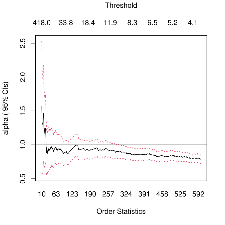
(a) Marine losses

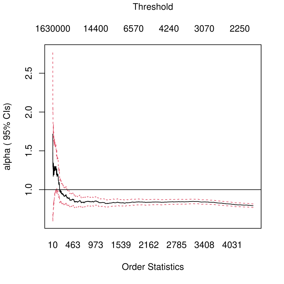
(b) Wildfire suppression costs

Figure 1: Hill plots for the marine losses and wildfire suppression costs: For each risk, the Hill estimates are plotted as black curve with the $95\%$ confidence intervals being red curves.

These observations suggest that the two loss datasets may have similar tail parameters. As one example of super-Pareto distributions, the generalized Pareto distribution when $\xi\geq 1$, is given by

$$G_{\xi,\beta}(x)=1-\left(1+\xi\frac{x}{\beta}\right)^{-1/\xi},~{}~{}~{}x\geq 0,$$

where $\beta>0$. By Theorem 1, if two loss random variables $X_{1}$ and $X_{2}$ are independent and follow generalized Pareto distributions with the same tail parameter $\alpha=1/\xi<1$, then, for all $p\in(0,1)$,

$$\mathrm{VaR}_{p}(X_{1}+X_{2})>\mathrm{VaR}_{p}(X_{1})+\mathrm{VaR}_{p}(X_{2}).$$ (17)

Even if $X_{1}$ and $X_{2}$ are not Pareto distributed, as long as their tails are Pareto, (17) may hold for $p$ relatively large, as suggested by Proposition 3.

We will verify (17) on our datasets to show how the implication of Theorem 1 holds for real data. Since the marine losses data were scaled to mask the actual losses, we renormalize it by multiplying the data by 500 to make it roughly on the same scale as that of the wildfire suppression costs; this normalization is made only for better visualization. Let $\widehat{F}_{1}$ be the empirical distribution of the marine losses (renormalized) and $\widehat{F}_{2}$ be the empirical distribution of the wildfire suppression costs. Take independent random variables $\widehat{Y}_{1}\sim\widehat{F}_{1}$ and $\widehat{Y}_{2}\sim\widehat{F}_{2}$. Let $\widehat{F}_{1}\oplus\widehat{F}_{2}$ be the distribution with quantile function $p\mapsto\mathrm{VaR}_{p}(\widehat{Y}_{1})+\mathrm{VaR}_{p}(\widehat{Y}_{2})$, i.e., the comonotonic sum, and $\widehat{F}_{1}*\widehat{F}_{2}$ be the distribution of $\widehat{Y}_{1}+\widehat{Y}_{2}$, i.e., the independent sum.

The differences between the distributions $\widehat{F}_{1}\oplus\widehat{F}_{2}$ and $\widehat{F}_{1}*\widehat{F}_{2}$ can be seen in Figure 2. We observe that $\widehat{F}_{1}*\widehat{F}_{2}$ is less than $\widehat{F}_{1}\oplus\widehat{F}_{2}$ over a wide range of loss values. In particular, the relation holds for all losses less than 267,659.5 (marked by the vertical line in Figure 2). Equivalently, we can see from Figure 2 that

$$\mathrm{VaR}_{p}(\widehat{Y}_{1}+\widehat{Y}_{2})>\mathrm{VaR}_{p}(\widehat{Y}_{1})+\mathrm{VaR}_{p}(\widehat{Y}_{2})$$ (18)

holds unless $p$ is greater than $0.9847$ (marked by the vertical line in Figure 2). Recall that $\widehat{F}_{1}*\widehat{F}_{2}\leq\widehat{F}_{1}\oplus\widehat{F}_{2}$ is equivalent to (18) holding for all $p\in(0,1)$. Since the quantiles are directly computed from data, thus from distributions with bounded supports, for $p$ close enough to $1$ it must hold that $\mathrm{VaR}_{p}(\widehat{Y}_{1}+\widehat{Y}_{2})\leq\mathrm{VaR}_{p}(\widehat{Y}_{1})+\mathrm{VaR}_{p}(\widehat{Y}_{2})$. Nevertheless, we observe (18) for most values of $p\in(0,1)$. Note that the observation of (18) is entirely empirical and it does not use any fitted models.

Let $F_{1}$ and $F_{2}$ be the true distributions (unknown) of the marine losses (renormalized) and wildfire suppression costs, respectively. We are interested in whether the first-order stochastic dominance relation $F_{1}*F_{2}\leq F_{1}\oplus F_{2}$ holds. Since we do not have access to the true distributions, we generate two independent random samples of size $10^{4}$ (roughly equal to the sum of the sizes of the datasets, thus with a similar magnitude of randomness) from the distributions $\widehat{F}_{1}\oplus\widehat{F}_{2}$ and $\widehat{F}_{1}*\widehat{F}_{2}$. We treat these samples as independent random samples from $F_{1}\oplus F_{2}$ and $F_{1}*F_{2}$ and test the hypothesis using Proposition 1 of Barrett and Donald (2003). The p-value of the test is greater than $0.5$ and we are not able to reject the hypothesis $F_{1}*F_{2}\leq F_{1}\oplus F_{2}$.

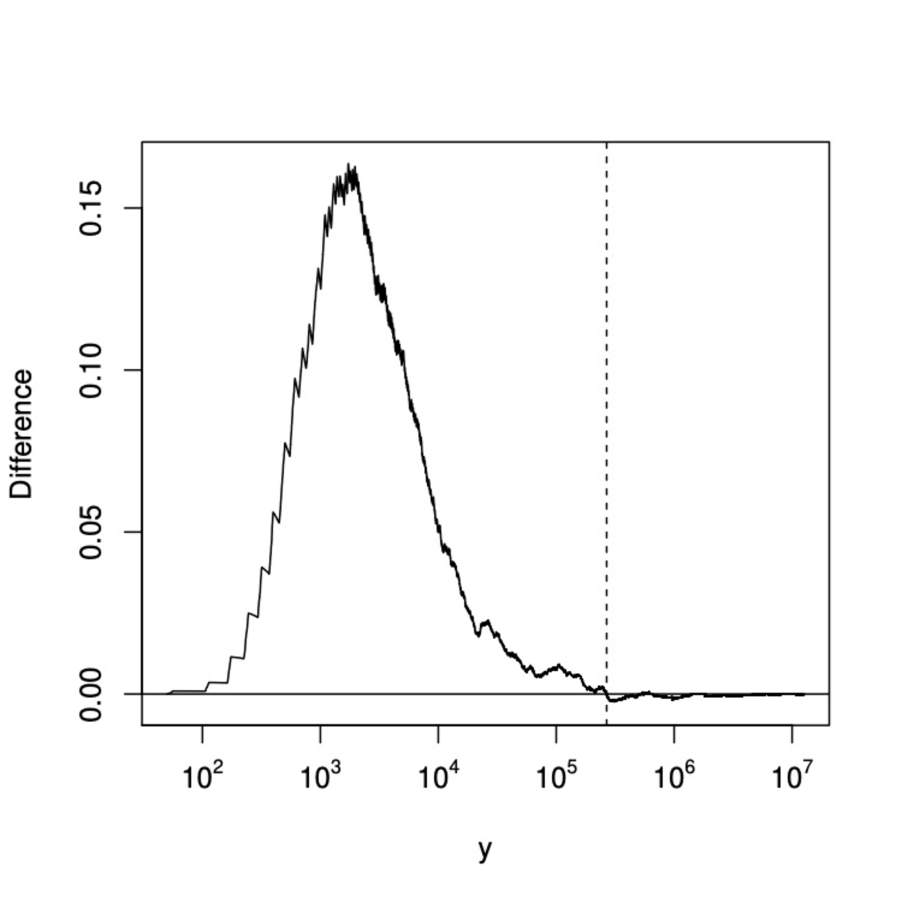
(a) Differences of the distributions: $\widehat{F}_{1}\oplus\widehat{F}_{2}-\widehat{F}_{1}*\widehat{F}_{2}$

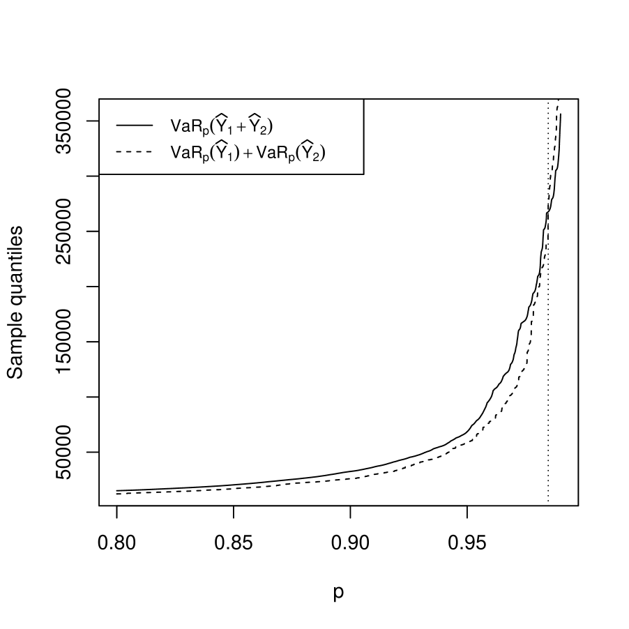
(b) Sample quantiles for $p\in(0.8,0.99)$

Figure 2: Plots for $\widehat{F}_{1}\oplus\widehat{F}_{2}-\widehat{F}_{1}*\widehat{F}_{2}$ and sample quantiles

6.2 Aggregation of Pareto risks with different parameters

As mentioned above, for independent losses $Y_{1},\dots,Y_{n}$ following generalized Pareto distributions with the same tail parameter $\alpha=1/\xi<1$, it holds that

$$\sum_{i=1}^{n}\mathrm{VaR}_{p}(Y_{i})\leq\mathrm{VaR}_{p}\left(\sum_{i=1}^{n}Y_{i}\right),\mbox{~{}usually with strict inequality}.$$ (19)

Inspired by the results in Section 6.1, we are interested in whether (19) holds for losses following generalized Pareto distributions with different parameters. To make a first attempt on this problem, we look at the 6 operational losses of different business lines with infinite mean in Table 5 of Moscadelli, (2004), where the operational losses are assumed to follow generalized Pareto distributions. Denote by $Y_{1},\dots,Y_{6}$ the operational losses corresponding to these 6 generalized Pareto distributions. The estimated parameters in Moscadelli, (2004) for these losses are presented in Table 1; they all have infinite mean.

$i$	1	2	3	4	5	6
$\xi_{i}$	1.19	1.17	1.01	1.39	1.23	1.22
$\beta_{i}$	774	254	233	412	107	243

Table 1: The estimated parameters $\xi_{i}$ and $\beta_{i}$, $i\in[6]$.

For the purpose of this numerical example, we assume that $Y_{1},\dots,Y_{6}$ are independent and plot $\sum_{i=1}^{6}\mathrm{VaR}_{p}(Y_{i})$ and $\mathrm{VaR}_{p}(\sum_{i=1}^{6}Y_{i})$ for $p\in(0.95,0.99)$ in Figure 3. We can see that $\mathrm{VaR}_{p}(\sum_{i=1}^{6}Y_{i})$ is larger than $\sum_{i=1}^{6}\mathrm{VaR}_{p}(Y_{i})$, and the gap between the two values gets larger as the level $p$ approaches 1. This observation further suggests that even if the extremely heavy-tailed Pareto losses have different tail parameters, a diversification penalty may still exist. We conjecture that this is true for any generalized Pareto losses $Y_{1},\dots,Y_{n}$ with shape parameters $\xi_{1},\dots,\xi_{n}\in[1,\infty)$, although we do not have a proof. Similarly, we may expect that $\sum_{i=1}^{n}\theta_{i}\mathrm{VaR}_{p}(X_{i})\leq\mathrm{VaR}_{p}(\sum_{i=1}^{n}\theta_{i}X_{i})$ holds for any Pareto losses $X_{1},\dots,X_{n}$ with tail parameters $\alpha_{1},\dots,\alpha_{n}\in(0,1]$,

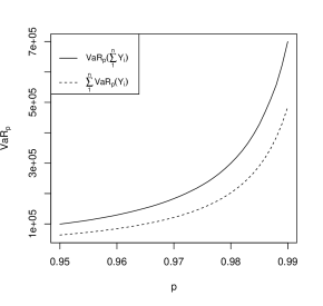
Figure 3: Curves of $\mathrm{VaR}_{p}(\sum_{i=1}^{n}Y_{i})$ and $\sum_{i=1}^{n}\mathrm{VaR}_{p}(Y_{i})$ for $n=6$ generalized Pareto losses with parameters in Table 1 and $p\in(0.95,0.99)$.

From a risk management point of view, the message from Sections 6.1 and 6.2 is clear. If a careful statistical analysis leads to statistical models in the realm of infinite means, then the risk manager at the helm should take a step back and question to what extent classical diversification arguments can be applied. Though we mathematically analyzed the case of identically distributed losses, we conjecture that these results hold more widely in the heterogeneous case. As a consequence, it is advised to hold on to only one such super-Pareto risk. Of course, the discussion concerning the practical relevance of infinite mean models remains. When such underlying models are methodologically possible, then one should think carefully about the applicability of standard risk management arguments; this brings us back to Weitzman’s Dismal Theorem as discussed towards the end of Section 1. From a methodological point of view, we expect that the results from Sections 4 and 5.2 carry over to the above heterogeneous setting.

7 Concluding remarks

We provide several generalizations of the inequality that the diversification of WNAID super-Pareto losses is greater than an individual super-Pareto loss in the sense of first-order stochastic dominance. The generalizations concern marginal distributions (Proposition 1), dependence structures (Proposition 2), a tail risk model (Proposition 3), a classic insurance model (Proposition 4), and bounded super-Pareto losses (Theorem 2). These results strengthen the main point made by Chen et al. (2024): As diversification increases the risk assessment of extremely heavy-tailed losses for all commonly used decision models, non-diversification is preferred.

The equilibrium of a risk exchange model is analyzed, where agents can take extra super-Pareto losses with compensations. In particular, if every agent is associated with an initial position of a super-Pareto loss, the agents can merely exchange their entire position with each other (Theorem 3). On the other hand, if some external agents are not associated with any initial losses, it is possible that all agents can reduce their risks by transferring the losses from the agents with initial losses to those without initial losses (Theorem 4).

Inspired by numerical results, an open question arises, that is whether

$$\mathrm{VaR}_{p}\left(\sum_{i=1}^{n}\theta_{i}X_{i}\right)\geq\sum_{i=1}^{n}\theta_{i}\mathrm{VaR}_{p}(X_{i})$$ (20)

holds for $(\theta_{1},\dots,\theta_{n})\in\Delta_{n}$ and independent extremely heavy-tailed Pareto losses $X_{1},\dots,X_{n}$ with possibly different tail parameters. From the numerical results in Section 6, (20) is anticipated to hold; a proof seems to be beyond the current techniques.

Acknowledgements

The authors thank Hansjörg Albrecher, Jan Dhaene, John Ery, Taizhong Hu, Massimo Marinacci, Alexander Schied, and Qihe Tang for helpful comments on a previous manuscript, which evolved into two papers (Chen et al. (2024) and this paper). RW is supported by the Natural Sciences and Engineering Research Council of Canada (RGPIN-2018-03823 and CRC-2022-00141).

Appendix A Background on risk measures

Recall that $\mathcal{X}_{\rho}$ is a convex cone of random variables representing losses faced by financial institutions. We first present commonly used properties of a risk measure $\rho:\mathcal{X}_{\rho}\rightarrow\mathbb{R}$:

1. Translation invariance: $\rho(X+c)=\rho(X)+c$ for $c\in\mathbb{R}$.

2. Positive homogeneity: $\rho(aX)=a\rho(X)$ for $a\geq 0$.

3. Convexity: $\rho(\lambda X+(1-\lambda)Y)\leq\lambda\rho(X)+(1-\lambda)\rho(Y)$ for $X,Y\in\mathcal{X}_{\rho}$ and $\lambda\in[0,1]$.

A risk measure that satisfies (b) weak monotonicity, (d) translation invariance, and (f) convexity is a convex risk measure (Föllmer and Schied,, 2002). ES is a convex risk measure. The convexity property means that diversification will not increase the risk of the loss portfolio, i.e., the risk of $\lambda X+(1-\lambda)Y$ is less than or equal to that of the weighted average of individual losses. However, the canonical space for law-invariant convex risk measures is $L^{1}$ (see Filipović and Svindland, (2012)) and hence convex risk measures are not useful for losses without finite mean.

For losses without finite mean, it is natural to consider VaR or Range Value-at-Risk (RVaR), which includes VaR as a limiting case. For $X\in\mathcal{X}$ and $0\leq p<q<1$, RVaR is defined as

$$\mathrm{RVaR}_{p,q}(X)=\frac{1}{q-p}\int_{p}^{q}\mathrm{VaR}_{u}(X)\mathrm{d}u.$$

For $p\in(0,1)$, $\lim_{q\downarrow p^{+}}\mathrm{RVaR}_{p,q}(X)=\mathrm{VaR}_{p}(X)$. The class of RVaR is proposed by Cont et al. (2010) as robust risk measures; see Embrechts et al. (2018) for its properties and risk sharing results. VaR, ES, RVaR, essential infimum ($\operatorname*{ess\text{-}inf}$), and essential supremum ($\operatorname*{ess\text{-}sup}$), belong to the family of distortion risk measures defined by (10). For $X\in\mathcal{X}$, $\operatorname*{ess\text{-}inf}$ and $\operatorname*{ess\text{-}sup}$ are defined as

$$\operatorname*{ess\text{-}inf}(X)=\sup\{x:F_{X}(x)=0\}~{}~{}~{}~{}\mbox{and}~{}~{}~{}~{}\operatorname*{ess\text{-}sup}(X)=\inf\{x:F_{X}(x)=1\}.$$

The distortion functions of $\operatorname*{ess\text{-}inf}$ and $\operatorname*{ess\text{-}sup}$ are $h(t)=\mathds{1}_{\{t=1\}}$ and $h(t)=\mathds{1}_{\{0<t\leq 1\}}$, $t\in[0,1]$, respectively; see Table 1 of Wang et al., (2020). Distortion risk measures satisfy (b), (d) and (e). Almost all useful distortion risk measures are mildly monotone, as shown by the following result.

Proposition A.1.

Any distortion risk measure is mildly monotone unless it is a mixture of $\operatorname*{ess\text{-}sup}$ and $\operatorname*{ess\text{-}inf}$.

Proof.

Let $\rho_{h}$ be a distortion risk measure with distortion function $h$. Suppose that $\rho_{h}$ is not mildly monotone. Then there exist $X,Y\in\mathcal{X}$ satisfying $F^{-1}_{X}(p)<F^{-1}_{Y}(p)$ for all $p\in(0,1)$ and $\rho(X)=\rho(Y)$. Suppose that there exist $b\in(0,1)$ such that $h(1-a)<h(1-b)$ for all $a>b$. For $x\in(F^{-1}_{X}(b),F^{-1}_{Y}(b))$, we have $F_{X}(x)\geq b>F_{Y}(x)$; see e.g., Lemma 1 of Guan et al. (2024). Hence, we have $h(1-F_{X}(x))\leq h(1-b)<h(1-F_{Y}(x))$ for $x\in(F^{-1}_{X}(b),F^{-1}_{Y}(b))$. Since $h(1-F_{X}(x))-h(1-F_{Y}(x))\leq 0$ for all $x\in\mathbb{R}$, by (10) we get

$$\rho(X)-\rho(Y)=\int_{-\infty}^{\infty}\left(h(1-F_{X}(x))-h(1-F_{Y}(x))\right)\mathrm{d}x<0.$$

This contradicts $\rho(X)=\rho(Y)$. Hence, there is no $b\in(0,1)$ such that $h(1-a)<h(1-b)$ for all $a>b$. Using a similar argument with the left quantiles replaced by right quantiles, we conclude that there is no $b\in(0,1)$ such that $h(1-a)>h(1-b)$ for all $a<b$. Therefore, for every $b\in(0,1)$, there exists an open interval $I_{b}$ such that $b\in I_{b}$ and $h$ is constant on $I_{b}$. For any $\epsilon>0$, the interval $[\epsilon,1-\epsilon]$ is compact. Hence, there exists a finite collection $\{I_{b}:b\in B\}$ which covers $[\epsilon,1-\epsilon]$. Since the open intervals in $\{I_{b}:b\in B\}$ overlap, we know that $h$ is constant on $[\epsilon,1-\epsilon]$. Letting $\epsilon\downarrow 0$ yields that $h$ takes a constant value on $(0,1)$, denoted by $\lambda\in[0,1]$. Together with $h(0)=0$ and $h(1)=1$, we get that $h(t)=\lambda\mathds{1}_{\{0<t\leq 1\}}+(1-\lambda)\mathds{1}_{\{t=1\}}$ for $t\in[0,1]$, which is the distortion function of $\rho_{h}=\lambda\operatorname*{ess\text{-}inf}+(1-\lambda)\operatorname*{ess\text{-}sup}$. ∎

As a consequence, for any set $\mathcal{X}$ containing a random variable unbounded from above and one unbounded from below, such as the $L^{q}$-space for $q\in[0,\infty)$, a real-valued distortion risk measure on $\mathcal{X}$ is always mildly monotone.

Appendix B Proofs of all results

Proof of Proposition 1.

To show that $\mathcal{F}_{\rm IN}$ is closed under convolution, note that first-order stochastic dominance is closed under convolution; see Theorem 1.A.3 of Shaked and Shanthikumar, (2007). Therefore, under independence,

$$X_{1j}\leq_{\rm st}\sum_{i=1}^{n}\theta_{i}X_{ij}\mbox{~{}for $j=1,2$}~{}\Longrightarrow~{}\sum_{j=1}^{2}X_{1j}\leq_{\rm st}\sum_{j=1}^{2}\sum_{i=1}^{n}\theta_{i}X_{ij}=\sum_{i=1}^{n}\theta_{i}\sum_{j=1}^{2}X_{ij}.$$

To show that $\mathcal{F}_{\rm IN}$ and $\mathcal{F}_{\rm WNA}$ are closed under strictly increasing convex transforms $f$, we note that if $Y\leq_{\rm st}\sum_{i=1}^{n}\theta_{i}Y_{i}$, then $f(Y)\leq_{\rm st}f(\sum_{i=1}^{n}\theta_{i}Y_{i})\leq\sum_{i=1}^{n}\theta_{i}f(Y_{i}),$ where the first inequality follows since $\leq_{\rm st}$ is preserved under increasing transforms, and the second inequality is due to convexity of $f$. Moreover, strictly increasing transforms do not affect the dependence structure of $(Y_{1},\dots,Y_{n})$. ∎

Proof of Proposition 2.

Copulas for independence and weak negative association are in $\mathcal{C}_{\mathrm{DP}}$ because of Theorem 1. The copula for comonotonicity is in $\mathcal{C}_{\mathrm{DP}}$ because $X_{1}=\sum_{i=1}^{n}\theta_{i}X_{i}$ almost surely in case of comonotonicity. Denote by $C$ a copula of $(X_{1},\dots,X_{n})$. Let $X\buildrel\mathrm{d}\over{=}X_{1}$. Then, there exists a random vector $(U_{1},\dots,U_{n})\sim C$ such that $(F_{X}^{-1}(U_{1}),\dots,F_{X}^{-1}(U_{n}))\buildrel\mathrm{d}\over{=}(X_{1},\dots,X_{n})$. Note that for $p\in(0,1)$, $\mathbb{P}(\sum_{i=1}^{n}\theta_{i}F_{X}^{-1}(U_{i})\leq p)$ is linear in the distribution of $(U_{1},\dots,U_{n})$. Therefore, if $\mathbb{P}(\sum_{i=1}^{n}\theta_{i}X_{i}\leq p)\leq\mathbb{P}(X\leq p)$ for all $p\in(0,1)$ holds for two different copulas, it also holds for their mixtures. ∎

Proof of Proposition 3.

Let $X_{1},\dots,X_{n}$ be iid super-Pareto random variables. Note that for $t\geq x$, by using Theorem 1 and $Y\geq_{\rm st}X$, we have

$$\mathbb{P}\left(\sum_{i=1}^{n}\theta_{i}Y_{i}>t\right)\geq\mathbb{P}\left(\sum_{i=1}^{n}\theta_{i}X_{i}>t\right)\geq\mathbb{P}\left(X>t\right)=\mathbb{P}\left(Y>t\right).$$

The statement on strictness also follows from Theorem 1. ∎

Proof of Proposition 4.

By Theorem 1, it is clear that $\mathbb{P}(\sum_{i=1}^{n}W_{i}X_{i}/\sum_{i=1}^{n}W_{i}\leq t)<\mathbb{P}(X\leq t)$ for $t>z_{X}$, $n\in\mathbb{N}/\{1\}$. As $N$ is independent of $\{W_{i}X_{i}\}_{i\in\mathbb{N}},$ for $t>z_{X}$,

$$\mathbb{P}\left(\frac{\sum_{i=1}^{N}W_{i}X_{i}}{\sum_{i=1}^{N}W_{i}}\leq t\right) =\mathbb{P}(N=0)+\sum_{n=1}^{\infty}\mathbb{P}\left(\frac{\sum_{i=1}^{n}W_{i}X_{i}}{\sum_{i=1}^{n}W_{i}}\leq t\right)\mathbb{P}(N=n)$$

$$\leq\mathbb{P}(N=0)+\mathbb{P}(N\geq 1)\mathbb{P}(X\leq t)=\mathbb{P}\left(X\mathds{1}_{\{N\geq 1\}}\leq t\right).$$

It is obvious that the inequality is strict if $\mathbb{P}(N\geq 2)\neq 0$. To show the second inequality in (3), note that for each realization of $N=n$ and $(W_{1},\dots,W_{N})=(w_{1},\dots,w_{n})\in\mathbb{R}^{n}$, $\sum_{i=1}^{n}w_{i}X\leq_{\rm st}{\sum_{i=1}^{n}w_{i}X_{i}}$ holds by Theorem 1. Hence, the second inequality in (3) holds. ∎

Proof of Theorem 2.

For $t\in(z_{X},c]$, we have

$$\mathbb{P}\left(\sum_{i=1}^{n}\theta_{i}Y_{i}\leq t\right) =\mathbb{P}\left(\sum_{i=1}^{n}\theta_{i}(X_{i}\wedge c_{i})\leq t\right)=\mathbb{P}\left(\sum_{i=1}^{n}\theta_{i}X_{i}\leq t\right).$$

We also have $\mathbb{P}(Y_{i}\leq t)=\mathbb{P}(X_{i}\wedge c_{i}\leq t)=\mathbb{P}(X_{i}\leq t)$, $i\in[n]$. By the strictness statement in Theorem 1, we obtain the probability inequality. To show the quantile inequality, note that for $p\in(0,\mathbb{P}(X\leq c))$, we have $\mathrm{VaR}_{p}(X)<c.$ Using Theorem 1 and the definition of $Y_{1},\dots,Y_{n}$, we get

$$\sum_{i=1}^{n}\theta_{i}\mathrm{VaR}_{p}(Y_{i})\leq\mathrm{VaR}_{p}(X) <\mathrm{VaR}_{p}\left(\sum_{i=1}^{n}\theta_{i}X_{i}\right)\wedge c$$

$$\leq\mathrm{VaR}_{p}\left(\left(\sum_{i=1}^{n}\theta_{i}X_{i}\right)\wedge c\right)\leq\mathrm{VaR}_{p}\left(\sum_{i=1}^{n}\theta_{i}Y_{i}\right).$$

This gives the desired inequality. ∎

Proof of Theorem 3.

1. Suppose that $\left(\mathbf{p}^{*},\mathbf{w}^{1*},\dots,\mathbf{w}^{n*}\right)$ forms an equilibrium. We let $p=\max_{j\in[n]}\{p_{j}\}$ and $S=\operatorname*{arg\,max}_{j\in[n]}\{p_{j}\}$. For agent $i$, by writing $w=\|\mathbf{w}^{i}\|$, using Theorem 1 and the fact that $\rho_{i}$ is mildly monotone, we have that for any $\mathbf{w}^{i}\in\mathbb{R}_{+}^{n}$,

   $$\rho_{i}(L_{i}(\mathbf{w}^{i},\mathbf{p}^{*})) =\rho_{i}(\mathbf{w}^{i}\cdot(\mathbf{X}-\mathbf{p}^{*})+\mathbf{a}^{i}\cdot\mathbf{p}^{*})$$

   $$\geq\rho_{i}(\mathbf{w}^{i}\cdot\mathbf{X}-wp+\mathbf{a}^{i}\cdot\mathbf{p}^{*})\geq\rho_{i}(wX_{1}-wp+\mathbf{a}^{i}\cdot\mathbf{p}^{*}).$$

   By the last statement of Theorem 1, the last inequality is strict if $\mathbf{w}^{i}$ contains at least two non-zero components. Moreover, $c(\|\mathbf{w}^{i}\|-\|\mathbf{a}^{i}\|)=c(w-\|\mathbf{a}^{i}\|)$. Therefore, the optimizer $\mathbf{w}^{i*}=(w_{1}^{i*},\dots,w_{n}^{i*})$ to (8) has at most one non-zero component $w_{j}^{i*}$ for $j\in S$. Hence, $w_{k}^{i*}=0$ if $k\in[n]\setminus S$ and this holds for each $i\in[n]$. Using $\sum_{i=1}^{n}\mathbf{w}^{i*}=\sum_{i=1}^{n}\mathbf{a}^{i}$ which have all positive components, we know that $S=[n]$, which further implies that $\mathbf{p}^{*}=\left(p,\dots,p\right)$ for $p\in\mathbb{R}_{+}$. Next, as each $\mathbf{w}^{i*}$ has only one positive component, $(\mathbf{w}^{1*},\dots,\mathbf{w}^{n*})$ has to be an $n$-permutation of $(\mathbf{a}^{1},\dots,\mathbf{a}^{n})$ in order to satisfy the clearance condition (9).

2. The clearance condition (9) is clearly satisfied. As distortion risk measures are translation invariant and positive homogeneous (see Appendix A), by Proposition 6, for $i\in[n]$,

   $$\min_{\mathbf{w}^{i}\in\mathbb{R}_{+}^{n}}\left\{\rho_{i}\left(L_{i}(\mathbf{w}^{i},\mathbf{p}^{*})\right)+c_{i}(\|\mathbf{w}^{i}\|-\|\mathbf{a}^{i}\|)\right\}$$

   $$=\min_{\mathbf{w}^{i}\in\mathbb{R}_{+}^{n}}\left\{\rho_{i}\left(\mathbf{w}^{i}\cdot\mathbf{X}-(\mathbf{w}^{i}-\mathbf{a}^{i})\cdot\mathbf{p}^{*}\right)+c_{i}(\|\mathbf{w}^{i}\|-\|\mathbf{a}^{i}\|)\right\}$$

   $$=\min_{\|\mathbf{w}^{i}\|\in\mathbb{R}_{+}}\left\{(\rho_{i}\left(\|\mathbf{w}^{i}\|X\right)-(\|\mathbf{w}^{i}\|-a_{i})p)+c_{i}(\|\mathbf{w}^{i}\|-\|\mathbf{a}^{i}\|)\right\}$$

   $$=\min_{w\in\mathbb{R}_{+}}\left\{w(\rho_{i}(X)-p)+a_{i}p+c_{i}(w-a_{i})\right\}.$$ (A.1)

   Note that $w\mapsto w(\rho_{i}(X)-p)+c_{i}(w-a_{i})$ is convex and with condition (11), its minimum is attained at $w=a_{i}$. Therefore, $\mathbf{w}^{i*}=\mathbf{a}^{i*}$ is an optimizer to (8), which shows the desired equilibrium statement.

3. By (i), $\left(\mathbf{w}^{1*},\dots,\mathbf{w}^{n*}\right)$ is an $n$-permutation of $(\mathbf{a}^{1},\dots,\mathbf{a}^{n})$. It means that for any $i\in[n]$, there exists $j\in[n]$ such that $a_{j}$ is the minimizer of (A.1). As $c_{i}$ is convex, we have

   $$c_{i+}^{\prime}(a_{j}-a_{i})\geq p-\rho_{i}(X)\geq c_{i-}^{\prime}(a_{j}-a_{i}),~{}~{}~{}~{}\mbox{for each}~{}~{}~{}~{}i\in[n].$$

   Hence, we obtain (12). ∎

Proof of Theorem 4.

As in Section 5.2, an optimal position for either the internal or the external agents is to concentrate on one of the losses $X_{i}$, $i\in[n]$. By the same arguments as in Theorem 3 (i), the equilibrium price, if it exists, must be of the form $\mathbf{p}=(p,\dots,p)$. For such a given $\mathbf{p}$, using the assumption that $\rho_{E}$ and $\rho_{I}$ are mildly monotone and Proposition 6, we can rewrite the optimization problems in (13) and (14) as

$${\min_{\mathbf{u}^{j}\in\mathbb{R}_{+}^{n}}}\left\{\rho_{E}\left(L_{E}(\mathbf{u}^{j},\mathbf{p})\right)+c_{E}(\|\mathbf{u}^{j}\|)\right\} ={\min_{u\in\mathbb{R}_{+}}}\left\{u\left(\rho_{E}\left(X\right)-p\right)+c_{E}(u)\right\},$$ (A.2)

and

$${\min_{\mathbf{w}^{i}\in\mathbb{R}_{+}^{n}}}\left\{\rho_{I}\left(L_{i}(\mathbf{w}^{i},\mathbf{p})\right)+c_{I}(\|\mathbf{w}^{i}\|-\|\mathbf{a}^{i}\|)\right\}={\min_{w\in\mathbb{R}_{+}}}\left\{w(\rho_{I}\left(X\right)-p)+ap+c_{I}(w-a)\right\},$$ (A.3)

for $j\in[m]$ and $i\in[n]$. Note that the derivative of the function inside the minimum of the right-hand side of (A.2) with respect to $u$ is $L_{E}(u)-p$, and similarly, $L_{I}(w-a)-p$ is the derivative of the function inside the minimum of the right-hand side of (A.3). Using strict convexity of $c_{E}$ and $c_{I}$, we get the following facts.

1. The optimizer $u$ to (A.2) has two cases:

   1. If $L_{E}(0)\geq p$, then $u=0$.

   2. If $L_{E}(0)<p$, then $u>0$ and $L_{E}(u)=p$.

2. The optimizer $w$ to (A.3) has four cases:

   1. If $L_{I}^{+}(0)<p$, then $w>a$. This is not possible in an equilibrium.

   2. If $L_{I}^{+}(0)\geq p\geq L_{I}^{-}(0)$, then $w=a$.

   3. If $L_{I}^{-}(0)>p>L_{I}(-a)$, then $0<w<a$ and $L_{I}(w-a)=p$.

   4. If $L_{I}(-a)\geq p$, then $w=0$.

From the above analysis, we see that the optimal positions for the external agents are either all $0$ or all positive, and they are identical due to the strict monotonicity of $L_{E}$. We can say the same for the internal agents. Suppose that there is an equilibrium. Let $u$ be the external agent’s common exposure, and $w$ be the internal agent’s exposure. By the clearance condition (15) we have $w+ku=a$. If $0<ku<a$, then from (1.b) and (2.c) above, we have $L_{E}(u)=L_{I}(-ku)$. Below we show the three statements.

1. The “if” statement is clear by (1.b) and (2.d). We show the “only if” statement. We first assume that $p\in(L_{I}(-a),L_{I}^{-}(0))$. Since we also have $p>L_{E}(a/k)>L_{E}(0)$, from (1.b) and (2.c), $u$ should satisfy $L_{E}(u)=L_{I}(-ku)$. However, by strict monotonicity of $L_{E}$ and $L_{I}$, there is no $u\in(0,a/k]$ such that $L_{E}(u)=L_{I}(-ku)$. Moreover, if $p\leq L_{E}(0)$ or $p\geq L_{I}^{-}(0)$, the clearance condition (15) cannot be satisfied. Therefore, we must have $L_{E}(0)<p\leq L_{I}(-a)$. In this case, $w=0$ by (2.d). Consequently, $u=a/k$ by the clearance condition (15) and (1.b) gives $p=L_{E}(a/k)$.

2. In this case, there exists a unique $u^{*}\in(0,a/k]$ such that $L_{E}(u^{*})=L_{I}(-ku^{*})$. It follows that $u=u^{*}$ optimizes (A.2) and $w=a-ku^{*}$ optimizes (A.3). It is straightforward to verify that $\mathcal{E}$ is an equilibrium, and thus the “if” statement holds. To show the “only if” statement, it suffices to notice that $L_{E}(u)=L_{I}(-ku)=p$ has to hold, where $p$ is an equilibrium price and $u$ is the optimizer to (A.2), and such $u$ and $p$ are unique. Next, we show the “only if” statement for $u^{*}<a/2k$. As the optimal position for each external agent is $a-ku^{*}>a/2$, if more than two internal agents take the same loss, then the clearance condition (15) does not hold. Hence, the internal agents have to take different losses. Moreover, as the optimal position for the internal agents are the same, the loss $X_{i}$ for each $i\in[n]$, must be shared by one internal and $k$ external agents. The equilibrium is preserved under permutations of allocations. Thus, we have the “only if ” statement for $u^{*}<a/2k$. The “if” statement is obvious.

3. The “if” statement can be verified directly by using Theorem 3 (ii). Next, we show the “only if” statement. By (2.a), it is clear that the equilibrium price $p$ satisfies $p\leq L_{I}^{+}(0)$. If $p<L_{I}^{-}(0)$, by (1.a), (2.c), and (2.d), the clearance condition (15) cannot be satisfied. Thus, $p\geq L_{I}^{-}(0)$. By a similar argument, we have $p\leq L_{E}(0)$. Hence, we get $p\in[L_{I}^{-}(0),L_{E}(0)\wedge L_{I}^{+}(0)]$. From (1.a) and (2.b), we have $u=0$ and $w=a$ and thus the desired result. ∎

Proof of Proposition 7.

The clearance condition (9) is clearly satisfied. As ES is translation invariant, it suffices to show that $\mathbf{w}^{i*}$ minimizes $\mathrm{ES}_{q}(\mathbf{w}^{i}\cdot\mathbf{X}-\mathbf{w}^{i}\cdot\mathbf{p}^{*})+c_{i}(\|\mathbf{w}^{i}\|-\|\mathbf{a}^{i}\|)$ for $i\in[n]$. Write $r:\mathbf{w}\mapsto\mathrm{ES}_{q}\left(\mathbf{w}\cdot\mathbf{X}\right)$ for $\mathbf{w}=(w_{1},\dots,w_{n})\in[0,1]^{n}$. By Corollary 4.2 of Tasche, (2000),

$$\frac{\partial r}{\partial w_{i}}\left(\mathbf{w}\right) =\mathbb{E}\left[X_{i}|A_{\mathbf{w}}\right],\mbox{~{}~{}~{}}i\in[n],$$

where $A_{\mathbf{w}}=\{\sum_{i=1}^{n}w_{i}X_{i}\geq\mathrm{VaR}_{q}\left(\sum_{i=1}^{n}w_{i}X_{i}\right)\}$. Moreover, using convexity of $r$, we have (see McNeil et al., (2015, p. 321))

$$r\left(\mathbf{w}\right)-\mathbf{w}\cdot\mathbf{p}^{*}\geq\sum_{i=1}^{n}w_{i}\frac{\partial r}{\partial w_{i}}(a_{1},\dots,a_{n})-\mathbf{w}\cdot\mathbf{p}^{*}=0.$$

By Euler’s rule (see McNeil et al., (2015, (8.61))), the equality holds if $\mathbf{w}=\lambda(a_{1},\dots,a_{n})$ for any $\lambda>0$ . By taking $\lambda=a_{i}/\sum_{j=1}^{n}a_{j}$, we get $\|\mathbf{w}\|=a_{i}=\|\mathbf{a}^{i}\|$, and hence $c_{i}(\|\mathbf{w}\|-\|\mathbf{a}^{i}\|)$ is minimized by $\mathbf{w}=\lambda(a_{1},\dots,a_{n})$. Therefore, $\mathbf{w}^{i*}$ is an optimizer for each $i\in[n]$. ∎

References

- Alam and Saxena (1981) Alam, K. and Saxena, K. M. L. (1981). Positive dependence in multivariate distributions. Communications in Statistics-Theory and Methods, 10(12):1183–1196.
- Artzner et al. (1999) Artzner, P., Delbaen, F., Eber, J.-M. and Heath, D. (1999). Coherent measures of risk. Mathematical Finance, 9(3):203–228.
- Axtell, (2001) Axtell, R. L. (2001). Zipf distribution of U.S. firm sizes. Science, 293:1818–1820.
- Balkema and de Haan, (1974) Balkema, A. and de Haan, L. (1974). Residual life time at great age. Annals of Probability, 2:792–804.
- Barrett and Donald (2003) Barrett, G. F. and Donald, S. G. (2003). Consistent tests for stochastic dominance. Econometrica, 71(1):71–104.
- Beirlant et al., (1999) Beirlant, J., Dierckx, G., Goegebeur, Y. and Matthys, G. (1999). Tail index estimation and an exponential regression model. Extremes, 2(2):177–200.
- Biffis and Chavez, (2014) Biffis, E. and Chavez, E. (2014). Tail risk in commercial property insurance. Risks, 2(4):393–410.
- Block et al., (1982) Block, H. W., Savits, T. H. and Shaked, M. (1982). Some concepts of negative dependence. Annals of Probability, 10(3): 765–772.
- Block et al., (1985) Block, H. W., Savits, T. H. and Shaked, M. (1985). A concept of negative dependence using stochastic ordering. Statistics and Probability Letters, 3(2):81–86.
- Chen et al. (2024) Chen, Y., Embrechts, P. and Wang, R. (2024). An unexpected stochastic dominance: Pareto distributions, dependence, and diversification. Operations Research, forthcoming.
- Cheynel et al., (2024) Cheynel, E., Cianciaruso, D. and Zhou, F. (2024). Fraud power laws. Journal of Accounting Research, forthcoming.
- Cirillo and Taleb, (2020) Cirillo, P. and Taleb, N. N. (2020). Tail risk of contagious diseases. Nature Physics, 16(6):606–613.
- Clark, (2013) Clark, D. R. (2013). A note on the upper-truncated Pareto distribution. Casualty Actuarial Society E-Forum, Winter, 2013, Volume 1, pp. 1–22.
- Cont et al. (2010) Cont, R., Deguest, R. and Scandolo, G. (2010). Robustness and sensitivity analysis of risk measurement procedures. Quantitative Finance, 10(6):593–606.
- Eling and Schnell, (2020) Eling, M. and Schnell, W. (2020). Capital requirements for cyber risk and cyber risk insurance: An analysis of Solvency II, the US risk-based capital standards, and the Swiss Solvency Test. North American Actuarial Journal, 24(3):370–392.
- Eling and Wirfs, (2019) Eling, M. and Wirfs, J. (2019). What are the actual costs of cyber risk events? European Journal of Operational Research, 272(3):1109–1119.
- Embrechts et al. (1997) Embrechts, P., Klüppelberg, C. and Mikosch, T. (1997). Modelling Extremal Events for Insurance and Finance. Springer, Heidelberg.
- Embrechts et al., (1999) Embrechts, P., Resnick, S. I. and Samorodnitsky, G. (1999). Extreme value theory as a risk management tool. North American Actuarial Journal, 3(2):30–41.
- Embrechts et al. (2009) Embrechts, P., Lambrigger, D. and Wüthrich, M. (2009). Multivariate extremes and the aggregation of dependent risks: examples and counter-examples. Extremes, 12(2):107–127.
- Embrechts et al. (2018) Embrechts, P., Liu, H. and Wang, R. (2018). Quantile-based risk sharing. Operations Research, 66(4):936–949.
- Filipović and Svindland, (2012) Filipović, D. and Svindland, G. (2012). The canonical model space for law-invariant convex risk measures is . Mathematical Finance, 22(3):585–589.
- FINMA, (2021) FINMA (2021). Standardmodell Versicherungen (Standard Model Insurance): Technical description for the SST standard model non-life insurance (in German), October 31, 2021, www.finma.ch.
- Flyvbjerg et al., (2022) Flyvbjerg, B., Budzier, A., Lee, J. S., Keil, M., Lunn, D. and Bester, D. W. (2022). The empirical reality of IT project cost overruns: Discovering a power-law distribution. Journal of Management Information Systems, 39(3):607–639.
- Föllmer and Schied, (2002) Föllmer, H. and Schied, A. (2002). Convex measures of risk and trading constraints. Finance and Stochastics, 6(4):429–447.
- Föllmer and Schied (2016) Föllmer, H. and Schied, A. (2016). Stochastic Finance. An Introduction in Discrete Time. Fourth Edition. Walter de Gruyter, Berlin.
- Guan et al. (2024) Guan, Y., Jiao, Z. and Wang, R. (2024). A reverse ES (CVaR) optimization formula. North American Actuarial Journal, forthcoming.
- Gabaix, (1999) Gabaix, X. (1999). Zipf’s law and the growth of cities. American Economic Review, 89(2):129–132.
- Gabaix and Ibragimov, (2011) Gabaix, X. and Ibragimov, R. (2011). Rank-1/2: A simple way to improve the OLS estimation of tail exponents. Journal of Business and Economic Statistics, 29(1):24–39.
- Hofert and Wüthrich, (2012) Hofert, M. and Wüthrich, M. V. (2012). Statistical review of nuclear power accidents. Asia-Pacific Journal of Risk and Insurance, 7(1), Article 1.
- Ibragimov et al., (2015) Ibragimov, M., Ibragimov, R. and Walden, J. (2015). Heavy-Tailed Distributions and Robustness in Economics and Finance, Vol. 214 of Lecture Notes in Statistics, Springer.
- Ibragimov et al. (2009) Ibragimov, R., Jaffee, D. and Walden, J. (2009). Non-diversification traps in markets for catastrophic risk. Review of Financial Studies, 22:959–993.
- Ibragimov et al. (2011) Ibragimov, R., Jaffee, D. and Walden, J. (2011). Diversification disasters. Journal of Financial Economics, 99(2):333–348.
- Ibragimov and Walden (2007) Ibragimov, R. and Walden, J. (2007). The limits of diversification when losses may be large. Journal of Banking and Finance, 31(8):2551–2569.
- Joag-Dev and Proschan (1983) Joag-Dev, K. and Proschan, F. (1983). Negative association of random variables with applications. Annals of Statistics, 11(1):286–295.
- Klugman et al. (2012) Klugman, S. A., Panjer, H. H. and Willmot, G. E. (2012). Loss Models: From Data to Decisions. 4th Edition. John Wiley & Sons.
- Lehmann (1966) Lehmann, E. L. (1966). Some concepts of dependence. Annals of Mathematical Statistics, 37(5):1137–1153.
- Markowitz (1952) Markowitz, H. (1952). The utility of wealth. Journal of Political Economy, 60(2):151–158.
- McNeil et al., (2015) McNeil, A. J., Frey, R. and Embrechts, P. (2015). Quantitative Risk Management: Concepts, Techniques and Tools. Revised Edition. Princeton University Press.
- Moscadelli, (2004) Moscadelli, M. (2004). The modelling of operational risk: Experience with the analysis of the data collected by the Basel committee. Technical Report 517. SSRN: 557214.
- Nelsen (2006) Nelsen, R. (2006). An Introduction to Copulas. Second Edition. Springer, New York.
- Nešlehová et al., (2006) Nešlehová, J., Embrechts, P. and Chavez-Demoulin, V. (2006). Infinite mean models and the LDA for operational risk. Journal of Operational Risk, 1(1):3–25.
- Nordhaus, (2009) Nordhaus, W. D. (2009). An analysis of the Dismal Theorem, Yale University: Cowles Foundation Discussion Paper 1686.
- OECD (2018) OECD. (2018). The Contribution of Reinsurance Markets to Managing Catastrophe Risk. Available at www.oecd.org.
- Pickands, (1975) Pickands, J. (1975). Statistical inference using extreme order statistics. Annals of Statistics, 3:119–131.
- Rizzo, (2009) Rizzo, M. L. (2009). New goodness-of-fit tests for Pareto distributions. ASTIN Bulletin, 39(2):691–715.
- Samuelson, (1967) Samuelson, P. A. (1967). General proof that diversification pays. Journal of Financial and Quantitative Analysis, 2(1):1–13.
- Shaked and Shanthikumar, (2007) Shaked, M. and Shanthikumar, J. G. (2007). Stochastic Orders. Springer.
- Silverberg and Verspagen, (2007) Silverberg, G. and Verspagen, B. (2007). The size distribution of innovations revisited: An application of extreme value statistics to citation and value measures of patent significance. Journal of Econometrics, 139(2):318–339.
- Sornette et al., (2013) Sornette, D., Maillart, T. and Kröger, W. (2013). Exploring the limits of safety analysis in complex technological systems. International Journal of Disaster Risk Reduction, 6:59–66.
- Tasche, (2000) Tasche, D. (2000). Conditional expectation as quantile derivative. arXiv: 0104190.
- Tversky and Kahneman (1992) Tversky, A. and Kahneman, D. (1992). Advances in prospect theory: Cumulative representation of Uncertainty. Journal of Risk and Uncertainty, 5(4): 297–323.
- Wang et al., (2020) Wang, Q., Wang, R. and Wei, Y. (2020). Distortion riskmetrics on general spaces. ASTIN Bulletin, 50(3):827–851.
- Weitzman (2009) Weitzman, M. L. (2009). On modeling and interpreting the economics of catastrophic climate change. Review of Economics and Statistics, 91(1):1-19.
- Yaari (1987) Yaari, M. E. (1987). The dual theory of choice under risk. Econometrica, 55(1):95–115.