SceneTracker: Long-term Scene Flow Estimation Network
Abstract
Considering the complementarity of scene flow estimation in the spatial domain’s focusing capability and 3D object tracking in the temporal domain’s coherence, this study aims to address a comprehensive new task that can simultaneously capture fine-grained and long-term 3D motion in an online manner: long-term scene flow estimation (LSFE). We introduce SceneTracker, a novel learning-based LSFE network that adopts an iterative approach to approximate the optimal trajectory. Besides, it dynamically indexes and constructs appearance and depth correlation features simultaneously and employs the Transformer to explore and utilize long-range connections within and between trajectories. With detailed experiments, SceneTracker shows superior capabilities in handling 3D spatial occlusion and depth noise interference, highly tailored to the LSFE task’s needs. The code for SceneTracker is available at https://github.com/wwsource/SceneTracker.
1 Introduction
The precise and online capture and analysis of fine-grained long-term 3D object motion play a pivotal role in scene comprehension. By accurately capturing the 3D movement of objects, detailed data on position, velocity, acceleration, and more can be obtained, allowing for an in-depth understanding of how objects move and interact within specific environments. This information holds critical significance across various domains, including robotics, autonomous driving, and virtual reality.
The existing work primarily focuses on scene flow estimation (SFE) and 3D object tracking (3D OT) tasks, which partially address the issue of online 3D motion capture. SFE aims to estimate the pixel-wise/point-wise 3D motion between consecutive stereo, RGB-D, or point cloud data, and it can capture fine-grained instantaneous 3D displacement. However, SFE is unable to capture the 3D trajectory over a period of time robustly. Due to the presence of occlusions, per-frame 3D displacements cannot form the trajectory through simple chaining. 3D OT aims to achieve long-term tracking of targets in point clouds and employs a 3D bounding box to mark the position and size of the target at each moment. It operates on the object level and provides limited information about 3D deformations within the object.
Considering the complementarity of scene flow estimation in the spatial domain’s focusing capability and 3D object tracking in the temporal domain’s coherence, this study aims to address a comprehensive new task that can simultaneously capture fine-grained and long-term 3D motion: long-term scene flow estimation (LSFE). LSFE seeks to estimate the query pixel/point’s 3D trajectory within a continuous stereo, RGB-D, or point cloud sequence online. Our task can be seen as an extension of SFE into a more extended temporal domain or an extension of 3D OT into the pixel/point-level spatial domain.
We propose SceneTracker, the first long-term scene flow estimation method, which takes a -frame RGB-D video and the camera intrinsics as input, along with the starting 3D coordinates and starting time of an arbitrary 3D target to track, and produces a matrix as output, representing the positions in the camera coordinate system of the target across the given frames. SceneTracker adopts an iterative approach to approximate the optimal trajectory, overcoming the significant displacement challenges between frames. Besides, it dynamically indexes and constructs appearance and depth correlation features simultaneously, enhancing the ability to localize the target 3D position. Finally, it employs the Transformer to explore and utilize long-range connections within and between trajectories, further improving the accuracy of long-term scene flow estimation.
Compared to the scene flow-based chaining method and tracking any point-based depth indexing method, the proposed SceneTracker is highly tailored to the needs of the LSFE task. It can effectively address 3D spatial occlusion and depth noise interference, achieving median 3D error reductions of 39.0% and 85.9%, respectively.
The study offers the following contributions:
-
To better capture the fine-grained and long-term 3D motion, a new task, long-term scene flow estimation, is studied.
-
A novel learning-based LSFE network, SceneTracker, is presented to estimate per-point 3D trajectory within an RGB-D video effectively.
-
Both qualitative and quantitative experiments are conducted to verify the validity of the proposed method.
2 Related Works
2.1 Optical Flow Estimation
Optical Flow Estimation (OFE) aims to estimate the pixel-wise 2D instantaneous motion between consecutive video frames. Many of its classic works have inspired approaches to solving the SFE task. FlowNet [2] is the first method using DNNs to estimate optical flow. After that, a series of methods, such as PWC-Net [17] and LiteFlowNet [4], adopt a pyramid structure to refine the estimated optical flow from coarse to fine. GMFlow [22] completely transforms the mainstream regression-based pipeline and reformulates the optical flow estimation problem as a global matching problem, identifying corresponding relationships by directly comparing feature similarities. RAFT [18] adopts an iterative method to continuously refine the optical flow results at the same high resolution and has achieved significant performance improvements. Since then, GMA [5] and SplatFlow [20] have optimized this single-resolution iterative method from a spatial or temporal perspective, further improving the accuracy.
2.2 Scene Flow Estimation
As a fundamental yet challenging problem in 3D computer vision, SFE has been extensively studied in recent years due to its numerous applications, including autonomous driving, human pose estimation, moving object segmentation, and many others. The existing methods generally rely on feature similarities as their underlying principle. FlowNet3D [9] operates directly on point clouds with PointNet++ [15]. CamLiFlow [8] refines the optical flow and scene flow from the two frames’ feature similarity tensor in a coarse-to-fine way with two branches. OpticalExp [23] uses optical expansion to recover the pixel’s motion in depth between frames. It can estimate the final depth value of the second frame by combining the first frame’s depth, indirectly estimating the scene flow per pixel. The existence of occlusion issues severely constrains the accuracy of SFE. To tackle the occlusion problem, RigidMask [24] and RAFT-3D [19] focus on introducing rigid motion priors explicitly and implicitly, respectively.
2.3 Tracking Any Point
Unlike OFE, which focuses on local instantaneous motion, the Tracking Any Point (TAP) task focuses more on the global motion trajectory in the image domain. PIPs [3] combines cost volumes and iterative inference with a deep temporal network, which jointly reasons about the location and appearance of visual entities across multiple timesteps, achieving excellent tracking results. TAP-Net [1] computes cost volumes for the first frame and each intermediate frame of the video independently, which will be directly used for regression of position and occlusion status. MFT [14] performs the chaining of optical flow and occlusion status by estimating the uncertainty. Cotracker [6] utilizes the strong correlation between multiple tracking points for joint tracking. PIPs++ [25] introduces 1D convolution and dynamic templates, improving the tracking survival rate over longer time spans. In contrast to the TAP task, LSF involves overcoming inherent noise in depth data and considering the 3D structure of objects and their motion patterns to accurately track trajectories in 3D space.
2.4 Reconstruction-based Offline Methods
Inspired by 3D-GS [7], which is notable for its pure explicit representation and differential point-based splatting method, many works have started to use 3D Gaussian to reconstruct dynamic scenes and render novel views. Dynamic 3D Gaussians [11] models dynamic scenes by tracking the position and variance of each 3D Gaussian at each timestamp. 4D-GS [21] proposes 4D Gaussian Splatting as a holistic representation for dynamic scenes rather than applying 3D-GS for each frame. After training on the complete multi-view videos, these methods calculate 3D trajectories based on the Gaussian deformations. In contrast to this offline approach, the LSFE task focuses more on challenging scenarios involving constrained observations, limited response time, and future uncertainty.
3 Proposed Method
In this section, the holistic architecture of our method is described in Section 3.1. Then, two key contributions of our method, including the Flow Iteration Module and the Transformer Cell network, are depicted in Section 3.2 and 3.3, respectively. Some details of the model during training and inference are provided in Section 3.4.
3.1 Overall Architecture of SceneTracker
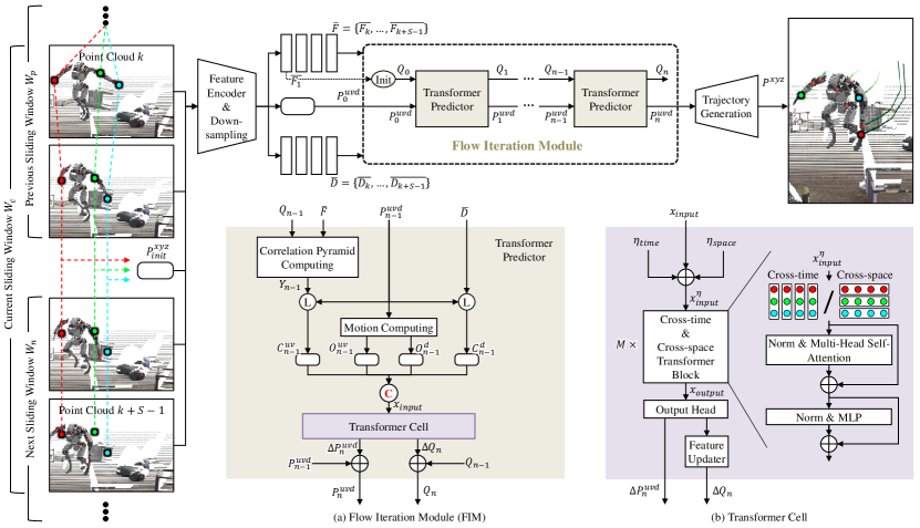
Our goal is to track 3D points throughout a 3D video. We formalize the problem as follows. A 3D video is a sequence of RGB frames along with their depth maps. Estimating the long-term scene flow amounts to producing the 3D trajectories in the camera coordinate system for query points with known initial positions. By default, all tracking starts from the first frame of the video. It is worth noting that our method can flexibly start tracking from any frame. The overall architecture of our method is shown in Fig. 1.
Trajectory initialization The first step of the initialization is to divide the entire video into several sliding windows. We partition it with a window size of and a sliding step of . As shown on the left side of Fig. 1, we need to track query points, taking the red, green, and blue points as examples.
For the first sliding window, the positions are initialized as the initial positions of the query points. For the other sliding windows, the first frames are initialized based on the estimated results of the last frames of the previous sliding window, and the last frames are all initialized based on the estimated result of the last frame of the previous sliding window. Notably, for the last sliding window, if its number of frames is less than , we will temporarily duplicate the last frame data to make up frames. Now, taking any current sliding window as an example, we can obtain the initialized trajectories .
Feature Encoder and downsampling Our network is performing inference at resolution . Here, is a downsampling factor utilized for efficiency. First, we use a Feature Encoder network to extract image features from in the current sliding window , assuming that ’s first frame is the entire video’s th frame. The Feature Encoder is a convolutional neural network comprising 8 residual blocks and 5 downsampling layers. The temporary features at 4 scales will generate a dense feature map at the input image resolution through scaling operations and convolutional layers.
Unlike processing RGB images, we directly take equidistant samples at intervals of from the -frame original depth maps, thereby obtaining the depth maps at of the original resolution. In addition, we transform from the camera coordinate system to a coordinate system composed of the plane and the depth dimension with the camera intrinsics , resulting in . The mathematical expressions of the conversion are as follows,
| (1) |
To match the generated and , we downsample the initialized trajectory to generate the :
| (2) |
Update of template feature and trajectory In the Flow Iteration Module, we iteratively update the query points’ template features and 3D trajectories. When processing the first sliding window’s first frame, we perform bilinear sampling on using the coordinates of the query points to obtain ’s initial template feature. Then, we replicate this feature times along the temporal dimension to obtain the initial template feature for all subsequent sliding windows. Each sliding window will have a consistent and different . After iterations of the same Transformer Predictor module, they will be updated to and .
Trajectory output We first upsample to generate to match the original input resolution:
| (3) |
Then, we combine the camera intrinsics to transform from the coordinate system to the camera coordinate system, resulting in . The mathematical expressions of the conversion are as follows,
| (4) |
Finally, we chain all estimated from the sliding windows. The overlapping parts between adjacent windows take the results from the latter window.
3.2 Flow Iteration Module
Like optical and scene flow, LSFE also faces the significant challenge of large inter-frame displacements. We draw on RAFT [18] and CoTracker [6], using an iterative approach to approximate the optimal result. At the same time, we use Transformer to model long-range dependencies within and between 3D trajectories of length . Finally, from a 2D perspective, we synchronize the extraction of the apparent and depth correlation features , which unifies the originally fragmented image and depth dimensions. Based on the above considerations, we design the Flow Iteration Module (FIM) for updating the template feature and trajectory , as shown in Fig. 1 (a).
Taking the FIM’s th iteration as an example, the Transformer Predictor network requires inputs , , , and to construct the input for a Transformer Cell, which involves concatenating the apparent correlation feature , the depth correlation feature , the apparent motion , and the depth motion . The Transformer Cell outputs residuals, and , to update and to and , serving as the output for the current iteration:
| (5) | ||||
| (6) |
Apparent correlation feature Before constructing the apparent correlation feature , a -layer correlation pyramid between and is calculated by taking the dot product between all pairs of feature vectors at the same frame time and pooling the last two dimensions. Then, the network uses to lookup to obtain . Specifically, is obtained through bilinear sampling of layer by layer with the grid size and then concatenating. Here, is the local neighborhood radius.
Depth correlation feature The network uses to lookup to obtain . Specifically, is obtained through bilinear sampling of ’s inverse depth map with the grid size , calculating the residual with the depth prediction ’s inverse, and concatenating. Here, and are the local neighborhood radii in the and directions.
Apparent and depth motion We obtain the apparent motion and the depth motion by calculating the differences in positions and depths between each frame and the first frame () of the current window :
| (7) | ||||
| (8) |
Here is the sinusoidal position encoding.
3.3 Transformer Cell Network
In the Transformer Cell network, we perform feature extraction and enhancement on the concatenated input feature and then predict the residuals and , as shown in Fig. 1 (b).
First, will be sinusoidally encoded separately in spatial and temporal dimensions to obtain and . Then, we perform element-wise addition on , , and to obtain . Afterward, will undergo Transformer Blocks for feature enhancement, with Cross-time and Cross-space Transformer Blocks being executed alternately. The two types of Transformer Blocks divide into tokens based on trajectories and time points, respectively. After tokenization, both types of Transformer Blocks will sequentially undergo a normalization layer, multi-head self-attention layer, normalization layer, and MLP layer, accompanied by two skip connections. The model can effectively explore and utilize long-range connections within and between trajectories through the operations above.
The final Transformer Block outputs , which is then fed into an Output Head network. The Output Head network comprises a fully connected layer, and its output can be split into and an intermediate feature. The intermediate feature will be input into a Feature Updater network, consisting of a normalization layer, a fully connected layer, and a GELU activation layer. The Feature Updater network outputs .
3.4 Training and Inference
Our method for training involves using a -frame 3D video as a data unit and the query points’ 3D trajectories to supervise the network’s outputs.
We supervise our network in an unrolled fashion to properly handle semi-overlapping sliding windows. is used to measure the error of trajectory prediction. Given the ground truth position and depth for any sliding window, we define the loss as follows (for simplicity, we omit the indices of the windows):
| (10) |
Here we set and . is the last sliding window.
4 Experiments
4.1 Datasets and Experimental Setup
4.1.1 Datasets
Unlike optical and scene flow tasks, LSFE lacks a dedicated dataset. For example, scene flow datasets such as FlyingThings3D [12] and KITTI2015 [13] only provide dense 3D point correspondences between adjacent frames. Although these datasets also provide 3D video data containing long-term information, the reference points change continuously as the video progresses.
The only dataset potentially supporting LSFE tasks is PointOdyssey [25], initially proposed for the TAP task. PointOdyssey is a large-scale synthetic dataset and data generation framework for the training and evaluating TAP methods. It aims to push the boundaries of what is possible by focusing on lengthy videos featuring realistic movements. PointOdyssey animates flexible characters using real-world motion capture data, constructs 3D environments corresponding to the motion capture settings, and generates camera perspectives using trajectories obtained through structure-from-motion applied to real videos to achieve this naturalism. It introduces variation by randomizing character attributes, motion characteristics, materials, lighting, 3D elements, and environmental effects.
Fortunately, it can selectively output the depth maps corresponding to RGB images and trajectories in the depth dimension, providing opportunities for training and evaluating LSFE methods. We construct an augmented dataset called LSFOdyssey based on the current PointOdyssey [25] dataset to tailor to LSFE tasks and reduce dataset reading time to expedite training. The LSFOdyssey dataset comprises 127,437 training data samples acquired through data augmentation techniques such as random flipping, spatial transformations, and color transformations. Each sample includes a 24-frame 3D video along with 3D trajectories of 256 query points. Furthermore, we ensure that all query points are non-occluded in at least the first four frames and a total of 12 frames in the video. Besides, we evenly partitioned 90 testing data samples without applying data augmentation techniques. Each sample consists of 40 frames and includes 256 query points. The entire LSFOdyssey dataset is approximately 240GB in size.
4.1.2 Evaluation Metrics
It is common to use metrics the average 2D position accuracy , the median 2D trajectory error , and the 2D “Survival” rate when evaluating the predicted 3D trajectory’s 2D performance. Here, quantifies the proportion of trajectory points falling within a specified distance threshold from the ground truth, averaged across thresholds , specified within a normalized resolution of . evaluates the percentage of frames in which the initial successful tracking occurs; tracking is deemed unsuccessful if the error exceeds 16 pixels in the normalized resolution.
In evaluating the 3D performance of trajectories, we employ the following configuration. We utilize s and their average value to measure the percentage of trajectory points within a threshold distance to ground truth. We use median 3D trajectory error and 3D end-point error to measure the distance between the estimated trajectories and ground truth trajectories. Similarly, we utilize metric , with a failure threshold set at .
4.1.3 Implementation Details
We use PyTorch to implement our method. We use the AdamW [10] as an optimizer and the One-cycle [16] as the learning rate adjustment strategy. We set , , , , , and . We evaluate our method after 4 FIM iterations, i.e., , and we set for the Transformer Cell network. We use the NVIDIA 3090 GPU for training and inference.
4.1.4 Training Processes
Our training includes a training process named Odyssey. We train the model on the LSFOdyssey dataset from scratch in the Odyssey training process. Each data sample learns 24 time frames and 256 query points. The input resolution is . The batch size is 8. The learning rate is , and the number of training steps is 200K.
4.2 Visualizations of Results
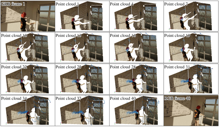
Following the Odyssey training process, we visualize the estimation results of SceneTracker on the LSFOdyssey test dataset, as shown in Fig. 2. We present the 14 frames of point clouds from the 40-frame test data sample at equal intervals and the RGB images of the first and last frames. The predicted 3D trajectories are depicted in blue on their corresponding point clouds. From Fig. 2, we can see that our method can consistently deliver smooth, continuous, and precise estimation results in the face of the complex motions of the camera and dynamic objects in the scene.
4.3 Comparisons with SF baseline
| Method | |||
|---|---|---|---|
| SF baseline | 75.11 | 92.81 | 4.90 |
| SceneTracker (Ours) | 85.33 | 96.80 | 2.02 |
We follow RAFT [18] to design a straightforward scene flow baseline named SF baseline. Since original scene flow methods can only address trajectory prediction problems between two frames, we adopt a chaining approach to handle long videos. Precisely, after calculating the scene flow between the first and second frames, we determine the coordinates corresponding to the predicted position of the second frame and index the depth of the second frame with these coordinates to obtain the query point coordinates from the second frame to the third frame, and so on for subsequent frames.
We also train the SF baseline on the LSFOdyssey dataset from scratch to ensure equity. We use the same training settings as the SceneTracker’s Odyssey training process. After training, we compare our SceneTracker with the SF baseline on the LSFOdyssey test dataset. The results are shown in Fig. 3, Table 1 and Table 2.
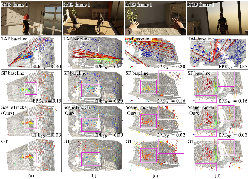
We can see from Table 1 and Table 2 that our method significantly outperforms the SF baseline across all dataset metrics, both in 2D and 3D domains. Especially on and , SceneTracker achieves error reductions of 58.8% and 39.0%, respectively. In contrast to the scene flow approach, our method employs identical query point features as initial templates tracked for each window, mitigating query point drift. This strategy effectively addresses occlusion and out-of-boundary effects, further substantiated in Fig. 3’s solid-box marked regions. The results fully demonstrate our method’s superior performance. The experimental findings substantiate the efficacy of our approach in tackling the LSF challenge.
4.4 Comparisons with TAP baseline
| Method | ||||||||
|---|---|---|---|---|---|---|---|---|
| TAP baseline | 42.43 | 57.45 | 67.52 | 74.20 | 60.40 | 49.37 | 0.389 | 0.575 |
| SF baseline | 53.22 | 71.78 | 84.40 | 92.67 | 75.52 | 83.38 | 0.123 | 0.132 |
| SceneTracker (Ours) | 64.67 | 79.88 | 90.85 | 96.67 | 83.02 | 89.25 | 0.075 | 0.081 |
We observe that our estimated 3D trajectories can be projected onto the image plane to form a continuous 2D trajectory, which serves as the output of the TAP task. For this purpose, we construct a TAP baseline based on SceneTracker. Specifically, the TAP baseline first outputs the image plane trajectory, then utilizes the trajectory to index into the depth map of each frame, and finally transforms the indexed trajectory into the camera coordinate system, as shown in Eq. 4.
We utilize SceneTracker trained through the Odyssey training process to provide 2D trajectories for the TAP baseline. After training, we compare our SceneTracker with the TAP baseline on the LSFOdyssey test dataset. The results are shown in Fig. 3 and Table 2.
We can see from Table 2 that our approach significantly outperforms the TAP baseline on all 3D dataset metrics. Especially on and , SceneTracker achieves error reductions of 80.7% and 85.9%, respectively. At the same time, on , SceneTracker achieves an 80.8% increase in accuracy. The significant performance gap stems mainly from the TAP baseline lacking robustness against depth noise interference and the inability to handle occlusion relationships in 3D space. It is worth noting that LSFOdyssey simulates fog and smoke, setting their depths as outliers directly, resulting in a depth map with a substantial amount of noise, posing significant challenges. The TAP baseline, due to its direct indexing from the depth map, is unable to detect and correct erroneous depth data, which is also substantiated in Fig. 3.
The results fully demonstrate that the proposed method excels in spatial relationship handling and noise resistance, highlighting the unique challenges the LSF task poses.
4.5 Ablation Studies
| Window Size | ||||||
|---|---|---|---|---|---|---|
| 8 | 83.17 | 96.29 | 2.89 | 78.35 | 86.51 | 0.102 |
| 12 | 84.68 | 96.51 | 2.22 | 81.47 | 88.08 | 0.083 |
| 16 | 85.33 | 96.80 | 2.02 | 83.02 | 89.25 | 0.075 |
| 20 | 84.48 | 96.50 | 2.11 | 53.21 | 58.03 | 0.197 |
| 24 | 83.93 | 96.31 | 2.26 | 44.75 | 47.80 | 0.232 |
We conduct a series of ablation experiments on our method from 2 aspects, which include the inference sliding window size, and the number of FIM’s updates, to examine their contributions. We use the model after Odyssey in all experiments and evaluate the LSFOdyssey test dataset.
4.5.1 Inference sliding window size
In Table 3, we inspect how the sliding window size of a model trained with sliding window affects model performance. We find that an inference window size achieves optimal performance across all dataset metrics, particularly all 3D metrics.
4.5.2 Number of FIM’s updates
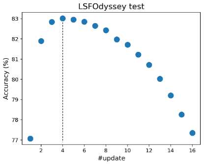
We train the model with FIM’s updates and evaluate with . The same inference update number gives the best results as evaluated in Fig. 4. The “Accuracy” represents the metric .
5 Conclusion
In summary, we propose a new task, i.e., long-term scene flow estimation, to better capture the fine-grained and long-term 3D motion. To effectively tackle this issue, we introduce a novel approach named SceneTracker. With detailed experiments, SceneTracker shows superior capabilities in handling 3D spatial occlusion and depth noise interference, highly tailored to the LSFE task’s needs.
Through this work, we further prove the feasibility of simultaneously capturing fine-grained and long-term 3D motion, and the LSFE task is poised to become a promising direction for future research.
References
- [1] Carl Doersch, Ankush Gupta, Larisa Markeeva, Adrià Recasens, Lucas Smaira, Yusuf Aytar, João Carreira, Andrew Zisserman, and Yi Yang. Tap-vid: A benchmark for tracking any point in a video. Advances in Neural Information Processing Systems, 35:13610–13626, 2022.
- [2] Alexey Dosovitskiy, Philipp Fischer, Eddy Ilg, Philip Hausser, Caner Hazirbas, Vladimir Golkov, Patrick Van Der Smagt, Daniel Cremers, and Thomas Brox. Flownet: Learning optical flow with convolutional networks. In ICCV, pages 2758–2766. IEEE, 2015.
- [3] Adam W Harley, Zhaoyuan Fang, and Katerina Fragkiadaki. Particle video revisited: Tracking through occlusions using point trajectories. In ECCV, pages 59–75. Springer, 2022.
- [4] Tak-Wai Hui, Xiaoou Tang, and Chen Change Loy. Liteflownet: A lightweight convolutional neural network for optical flow estimation. In CVPR, pages 8981–8989. IEEE, 2018.
- [5] Shihao Jiang, Dylan Campbell, Yao Lu, Hongdong Li, and Richard Hartley. Learning to estimate hidden motions with global motion aggregation. In ICCV, pages 9772–9781. IEEE, 2021.
- [6] Nikita Karaev, Ignacio Rocco, Benjamin Graham, Natalia Neverova, Andrea Vedaldi, and Christian Rupprecht. Cotracker: It is better to track together. arXiv preprint arXiv:2307.07635, 2023.
- [7] Bernhard Kerbl, Georgios Kopanas, Thomas Leimkühler, and George Drettakis. 3d gaussian splatting for real-time radiance field rendering. ACM Transactions on Graphics, 42(4), 2023.
- [8] Haisong Liu, Tao Lu, Yihui Xu, Jia Liu, Wenjie Li, and Lijun Chen. Camliflow: bidirectional camera-lidar fusion for joint optical flow and scene flow estimation. In CVPR, pages 5791–5801, 2022.
- [9] Xingyu Liu, Charles R Qi, and Leonidas J Guibas. Flownet3d: Learning scene flow in 3d point clouds. In CVPR, pages 529–537, 2019.
- [10] Ilya Loshchilov and Frank Hutter. Decoupled weight decay regularization. arXiv preprint arXiv:1711.05101, 2017.
- [11] Jonathon Luiten, Georgios Kopanas, Bastian Leibe, and Deva Ramanan. Dynamic 3d gaussians: Tracking by persistent dynamic view synthesis. arXiv preprint arXiv:2308.09713, 2023.
- [12] Nikolaus Mayer, Eddy Ilg, Philip Hausser, Philipp Fischer, Daniel Cremers, Alexey Dosovitskiy, and Thomas Brox. A large dataset to train convolutional networks for disparity, optical flow, and scene flow estimation. In CVPR, pages 4040–4048. IEEE, 2016.
- [13] Moritz Menze and Andreas Geiger. Object scene flow for autonomous vehicles. In CVPR, pages 3061–3070. IEEE, 2015.
- [14] Michal Neoral, Jonáš Šerỳch, and Jiří Matas. Mft: Long-term tracking of every pixel. In WACV, pages 6837–6847, 2024.
- [15] Charles Ruizhongtai Qi, Li Yi, Hao Su, and Leonidas J Guibas. Pointnet++: Deep hierarchical feature learning on point sets in a metric space. Advances in neural information processing systems, 30, 2017.
- [16] Leslie N Smith and Nicholay Topin. Super-convergence: Very fast training of neural networks using large learning rates. In Artificial intelligence and machine learning for multi-domain operations applications, volume 11006, pages 369–386. SPIE, 2019.
- [17] Deqing Sun, Xiaodong Yang, Ming-Yu Liu, and Jan Kautz. Pwc-net: Cnns for optical flow using pyramid, warping, and cost volume. In CVPR, pages 8934–8943. IEEE, 2018.
- [18] Zachary Teed and Jia Deng. Raft: Recurrent all-pairs field transforms for optical flow. In ECCV, pages 402–419. Springer, 2020.
- [19] Zachary Teed and Jia Deng. Raft-3d: Scene flow using rigid-motion embeddings. In CVPR, pages 8375–8384, 2021.
- [20] Bo Wang, Yifan Zhang, Jian Li, Yang Yu, Zhenping Sun, Li Liu, and Dewen Hu. Splatflow: Learning multi-frame optical flow via splatting. International Journal of Computer Vision, pages 1–23, 2024.
- [21] Guanjun Wu, Taoran Yi, Jiemin Fang, Lingxi Xie, Xiaopeng Zhang, Wei Wei, Wenyu Liu, Qi Tian, and Xinggang Wang. 4d gaussian splatting for real-time dynamic scene rendering. arXiv preprint arXiv:2310.08528, 2023.
- [22] Haofei Xu, Jing Zhang, Jianfei Cai, Hamid Rezatofighi, Fisher Yu, Dacheng Tao, and Andreas Geiger. Unifying flow, stereo and depth estimation. IEEE Transactions on Pattern Analysis and Machine Intelligence (TPAMI), 2023.
- [23] Gengshan Yang and Deva Ramanan. Upgrading optical flow to 3d scene flow through optical expansion. In CVPR, pages 1334–1343, 2020.
- [24] Gengshan Yang and Deva Ramanan. Learning to segment rigid motions from two frames. In CVPR, pages 1266–1275, 2021.
- [25] Yang Zheng, Adam W Harley, Bokui Shen, Gordon Wetzstein, and Leonidas J Guibas. Pointodyssey: A large-scale synthetic dataset for long-term point tracking. In ICCV, pages 19855–19865. IEEE, 2023.