On the Preprocessing of Physics-informed Neural Networks: How to Better Utilize Data in Fluid Mechanics

Abstract

Physics-Informed Neural Networks (PINNs) serve as a flexible alternative for tackling forward and inverse problems in differential equations, displaying impressive advancements in diverse areas of applied mathematics. Despite integrating both data and underlying physics to enrich the neural network’s understanding, concerns regarding the effectiveness and practicality of PINNs persist. Over the past few years, extensive efforts in the current literature have been made to enhance this evolving method, by drawing inspiration from both machine learning algorithms and numerical methods. Despite notable progressions in PINNs algorithms, the important and fundamental field of data preprocessing remain unexplored, limiting the applications of PINNs especially in solving inverse problems. Therefore in this paper, a concise yet potent data preprocessing method focusing on data normalization was proposed. By applying a linear transformation to both the data and corresponding equations concurrently, the normalized PINNs approach was evaluated on the task of reconstructing flow fields in three turbulent cases. The results, both qualitatively and quantitatively, illustrate that by adhering to the data preprocessing procedure, PINNs can robustly achieve higher prediction accuracy for all flow quantities through the entire training process, distinctly improving the utilization of limited training data. The proposed normalization method requires zero extra computational cost. Though only verified in Navier-Stokes (NS) equations, this method holds potential for application to various other equations.

I INTRODUCTION

Machine learning has rapidly permeated numerous domains over the last two decades, encompassing daily lifeKiran et al. (2021); Portugal, Alencar, and Cowan (2018) and scientific researchMorgan and Jacobs (2020); Greener et al. (2022); Brunton, Noack, and Koumoutsakos (2020), significantly changed our way of living and studying through the exploitation of vast datasets. Unlike pure data-driven approaches, Physics-informed Neural Networks is developed based on the concept of utilizing both data and underlying physical lawsKarniadakis et al. (2021); Cuomo et al. (2022). Originally conceived by LagarisLagaris, Likas, and Fotiadis (1998) and rekindled by RaissiRaissi, Perdikaris, and Karniadakis (2019), PINNs can now easily be deployed via popular machine learning framework such as TensorFlow and PyTorch. This method provides a flexible framework for solving both forward and inverse problemsYang, Meng, and Karniadakis (2021); Yu et al. (2022); Zhang et al. (2023) associated with differential equations, finding applications in diverse fields such as heat transferCai et al. (2021a); Jagtap, Mudunuru, and Nakshatrala (2023), seismologyRen et al. (2024), quantum physicsZhou and Yan (2021); Jin, Mattheakis, and Protopapas (2022) and fluid mechanicsCai et al. (2021b); Sharma et al. (2023).

Fluid mechanics, governed by the well-known Navier-Stokes equations and characterized by its nonlinear nature, stands out as a primary domain showcasing diverse applications of PINNs, ranging from laminar flowsRao, Sun, and Liu (2020); Biswas and Anand (2023) to turbulent flowsJin et al. (2021); Hanrahan, Kozul, and Sandberg (2023). Impressive examples include pressure and velocity inference from concentration field in cylinder wake and arteryRaissi, Yazdani, and Karniadakis (2020), pressure and velocity reconstruction from temperature fields over an espresso cupCai et al. (2021c), super-resolution and denoising of time resolved three-dimensional phase contrast magnetic resonance imaging (4D-Flow MRI)Fathi et al. (2020), etc. Despite the adaptability of PINNs in addressing both forward and inverse problems, given the convenience of automatic differentiationBaydin et al. (2018) in deep learning frameworks, and there have been evidence of successful flow simulation of PINNs without any labeled data in the training setSun et al. (2020). However, due to the unpredictable accuracy and prohibitive computational cost, the current nascent stage PINNs method is not comparable to traditional numerical algorithms in forward problems, leaving the superiority of PINNs mainly in inverse problems, where unknown flow features or undetermined parameters can be derived through abundant data or sparse data with ill-posed condition, which is also the focus of this paper.

A typical example of such inverse problems in fluid mechanics is flow field reconstruction, where incomplete or sparse data can be utilized by PINNs to reconstruct the unknown flow fieldXu et al. (2023a). Xu et al.Xu, Zhang, and Wang (2021) reconstructed the missing flow dynamics by treating the governing equations as a parameterized constraint. Wang et al. Wang et al. (2024) reconstructed the wake field of wind turbine using sparse LiDAR data. Xu et al.Xu et al. (2023b) reconstructed the cylinder wake and decaying turbulence using regularly distributed sparse data. Liu et al.Liu et al. (2024) reconstructed three-dimensional turbulent combustion with high-resolution using synthetic sparse data.

Despite the successful reconstructions mentioned above, the evolving method of PINNs still holds the potential to achieve tasks with increased accuracy and efficiency. In recent years, significant efforts have been dedicated to improving the trainability of PINNs, such as domain decompositionJagtap, Kharazmi, and Karniadakis (2020); Hu et al. (2023), parallel computingMeng et al. (2020); Xu et al. (2023b), adaptive sampling by respecting the causalityWang, Sankaran, and Perdikaris (2024), hybrid numerical schemeChiu et al. (2022), positional encoding for complex geometryCostabal, Pezzuto, and Perdikaris (2024), etc. While many of these improvements are developed by taking reference from traditional numerical methods, indeed PINNs can also be enhanced by adopting "tricks" from mainstream machine learning algorithms, such as adaptive activation functionJagtap, Kawaguchi, and Em Karniadakis (2020); Jagtap, Kawaguchi, and Karniadakis (2020), adaptive weightingMcClenny and Braga-Neto (2023), transfer learningXu et al. (2023c), etc. Among all these "tricks", one area that has received little attention in the realm of PINNs is data preprocessing.

As a fundamental technique in machine learning, data preprocessing methods such as data cleaning, data transformation, and data normalizationGarcía, Luengo, and Herrera (2015) have non-negligible effect on the performance of supervised learningKotsiantis, Kanellopoulos, and Pintelas (2006) and unsupervised learningGarcía et al. (2016). Among these methods, data normalization stands out as the most widely employed in various machine learning algorithms, aiming to scale all features to comparable level for more accurate learning. While analogous strategies, like incorporating non-dimensional equations, have been utilized in PINNs, and there has also been an expedient approach by adding a hidden normalization layer in the neural networks architectureRaissi, Yazdani, and Karniadakis (2020) (which would also be discussed in this paper). The effectiveness of data normalization in PINNs remains underexplored. Therefore in this paper, a data preprocessing pipeline focusing on normalization was proposed and evaluated on three test cases involving the reconstruction of unsteady flows with sparse data.

This article is organized as follows: Section II provides a detailed description of PINNs and the proposed normalization method on PINNs. In Section III, the three sparse datasets used in this study are introduced. Section IV demonstrates the superiority of the proposed preprocessing pipeline on three distinct problems, and Section V concludes the paper with a brief summary and discussion.

II METHODOLOGY

II.1 Physics informed neural networks

PINNs is a mesh-free approach for solving ordinary differential equationsDe Florio et al. (2024) and partial differential equationsMishra and Molinaro (2023). In addition to the conventional function of neural networks in data fitting, PINNs can further incorporate physical constraints: By configuring the independent variables as network input and the dependent variables as network output, the corresponding derivatives can be computed numerically by backtracking the computational graph. These derivatives are then combined with variables to construct the residuals of the differential equations. Subsequently, by integrating these residuals into the loss function, the physical laws can be imposed in a soft manner, as illustrated in Fig.1.

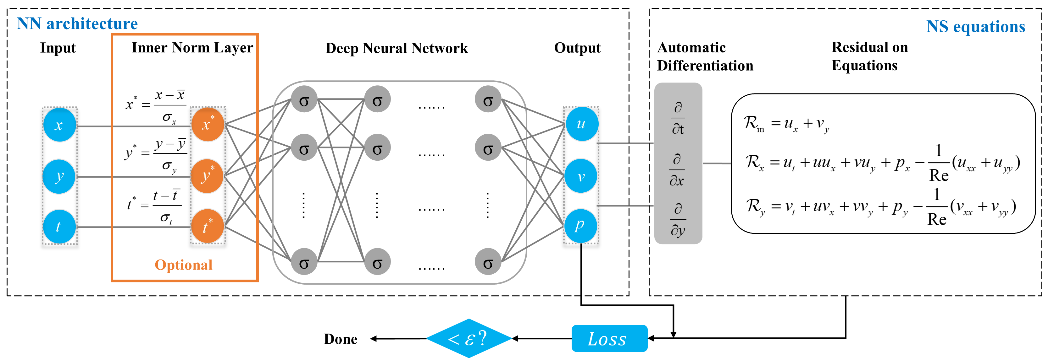
Figure 1: Physics-informed neural networks for solving non-dimensional NS equations. The loss function consists of both the data loss and the residual error of the conservation equations. $\sigma$ denotes the activation function. The inner normalization layer is an optional hidden layer that normalize the input features with z-score normalization, using mean and standard deviation values from the training set.

Given a neural network $\tilde{u}({\bf{x}};\theta)$, where $\bf{x}$ means the network input and $\theta$ means the undetermined weights and biases in the network, the composite loss function containing the data loss term and equation loss term can be written as

$$\zeta(\theta)={\zeta_{d}}(\theta)+\lambda_{r}\times{\zeta_{r}}(\theta)$$ (1)

where

$${\zeta_{d}}(\theta)=\frac{1}{{{N_{d}}}}\sum\limits_{i=1}^{{N_{d}}}{{{\left\|{\tilde{u}({\bf{x}}_{d}^{i};\theta)-{u_{d}^{i}}}\right\|}^{2}}}$$ (2)

$${\zeta_{r}}(\theta)=\frac{1}{{{N_{r}}}}\sum\limits_{i=1}^{Nr}{{{\left\|{{\bf{R}}(\tilde{u}({\bf{x}}_{r}^{i};\theta))}\right\|}^{2}}}$$ (3)

where $\{{\bf{x}}_{d}^{i},u_{d}^{i}\}_{i=1}^{{N_{d}}}$ is the training dataset with $N_{d}$ data points and $\{{\bf{x}}_{r}^{i}\}_{i=1}^{{N_{r}}}$ is the residual set with $N_{r}$ residual points (or called collocation points). $\lambda_{r}$ is a tunable hyper-parameter that allows the flexibility of assigning a different learning rate to each loss term and can also be a dynamic value that evolves with iterations to accelerate convergenceMaddu et al. (2022). Normally, $\lambda_{r}$ is set to 1. ${\bf{R}}(\tilde{u}({\bf{x}};\theta))$ is the residual vector of underlying differential equations. For 2-dimensional incompressible flow, ${\bf{R}}(\tilde{u}({\bf{x}};\theta))$ consists of ${\cal R}_{m}$, ${\cal R}_{x}$, and ${\cal R}_{y}$, whose non-dimensional form can be written as

$${{\cal R}_{m}}={u_{x}}+{v_{y}}$$ (4)

$${{\cal R}_{x}}={u_{t}}+u{u_{x}}+v{u_{y}}+{p_{x}}-\frac{1}{{{\mathop{\rm Re}\nolimits}}}({u_{xx}}+{u_{yy}})$$ (5)

$${{\cal R}_{y}}={v_{t}}+u{v_{x}}+v{v_{y}}+{p_{y}}-\frac{1}{{{\mathop{\rm Re}\nolimits}}}({v_{xx}}+{v_{yy}})$$ (6)

By minimizing Eq.1, PINNs can be made possible not only fitting the real data in the training set, but also satisfying the underlying physical principles, therefore capable of predicting unknown information of the flow field.

II.2 Normalization on Physics informed neural networks

Data normalization includes Min-Max normalization, Z-score normalization, and Decimal Scaling normalizationGarcía, Luengo, and Herrera (2015), where simple linear transformation is performed on both input features and output features. Taking Z-score normalization as an example. The features are normalized by first subtracting the mean values and then dividing the standard deviations, as shown in Eq. 7.

$${X^{*}}=\frac{{X-\bar{X}}}{{{\sigma_{X}}}}$$ (7)

By conducting Z-score normalization, the features are transformed to have a mean of 0 and a standard deviation of 1, as depicted in Figure 2. Since Z-score normalization is the most commonly employed method and shares the same mathematical foundation with other normalization techniques, this paper exclusively concentrates on Z-score normalization, hereafter referred to simply as "normalization."

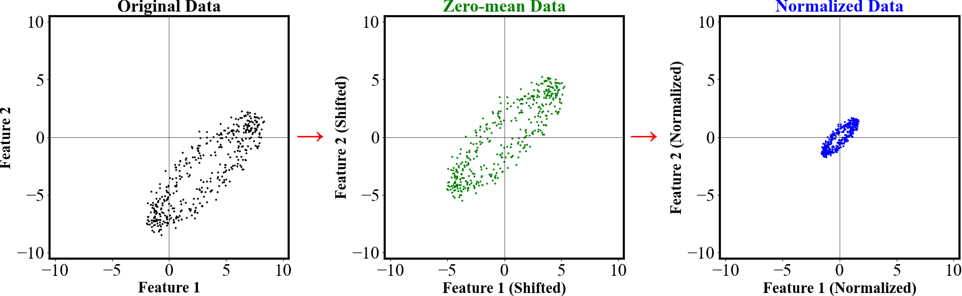
Figure 2: Two-dimensional illustration of Z-score normalization. Left: original data. Middle: the data has zero mean by subtracting the mean value on each dimension. Right: the data further has standard deviation of 1 by dividing the standard deviation of original data.

II.2.1 Inner normalization layer

For conventional pure data-driven neural networks, both the input and output features can undergo simultaneous normalization using the transformation specified in Eq.7. The model can then be trained on these normalized features, requiring only a subsequent denormalization step to revert to the original mapping. In contrast, for PINNs, the features cannot be normalized since each input and output feature has its own physical meaning. Applying normalization directly to PINNs would would only result in inconsistencies between the data and underlying equations.

An expedient approach that has been presented in some popular open source repositoriesRaissi, Yazdani, and Karniadakis (2020) involves incorporating a hidden layer, referred to as the inner normalization layer, immediately following the input layer. This inner normalization layer, depicted in the optional orange box in Fig.1, normalizes the input data using the mean and standard deviation values computed from the entire training dataset according to Eq.7. However, such expediency solely normalizes the input data within the neural network, leaving the output data in their original state. Furthermore, since the computational graph required for derivative calculation remains within the original input-output framework, the efficacy of the inner normalization layer is debatable.

II.2.2 Data normalization and equation transformation

While direct data normalization on PINNs may violate the fundamental physical constraints, the essence of normalization involving separate linear transformations for each variable is evident. Therefore, upon appropriately transforming the corresponding equations, data normalization can still be applicable.

Considering all dependent variables and independent variables $\Psi={[x,y,t,u,v,p]^{T}}$ in the non-dimensional equations given by Eq.4-6, normalization can be achieved using mean values $\bar{\Psi}={[\bar{x},\bar{y},\bar{t},\bar{u},\bar{v},\bar{p}]^{T}}$ and standard deviation values ${\sigma_{\Psi}}={[{\sigma_{x}},{\sigma_{y}},{\sigma_{t}},{\sigma_{u}},{\sigma_{v}},{\sigma_{p}}]^{T}}$ computed from the training dataset. By applying Eq.7, the normalized variables ${\Psi^{*}}={[{x^{*}},{y^{*}},{t^{*}},{u^{*}},{v^{*}},{p^{*}}]^{T}}$ can be obtained, making the normalized training data has mean of zero and standard deviation of 1 in each variable. Subsequently, utilizing a simple calculus technique outlined in Eq.8, Eq.4-6 can be transformed into Eq.9-11.

$$\frac{{{\partial^{n}}(ay+b)}}{{\partial{{(x+d)}^{n}}}}=\frac{{a{\partial^{n}}y}}{{{c^{n}}\partial{x^{n}}}}$$ (8)

$${{\cal R}_{m}}^{*}=\frac{{{\sigma_{u}}}}{{{\sigma_{x}}}}{u^{*}}_{{x^{*}}}+\frac{{{\sigma_{v}}}}{{{\sigma_{y}}}}{v^{*}}_{{y^{*}}}$$ (9)

$$\begin{split}{{\cal R}_{x}}^{*}=\frac{{{\sigma_{u}}}}{{{\sigma_{t}}}}{u^{*}}_{{t^{*}}}+\hat{u}\frac{{{\sigma_{u}}}}{{{\sigma_{x}}}}{u^{*}}_{{x^{*}}}+\hat{v}\frac{{{\sigma_{u}}}}{{{\sigma_{y}}}}{u^{*}}_{{y^{*}}}+\frac{{{\sigma_{p}}}}{{{\sigma_{x}}}}{p^{*}}_{{x^{*}}}\\ -\frac{1}{{{\mathop{\rm Re}\nolimits}}}(\frac{{{\sigma_{u}}}}{{{\sigma_{x}}^{2}}}{u^{*}}_{{x^{*}}{x^{*}}}+\frac{{{\sigma_{u}}}}{{{\sigma_{y}}^{2}}}{u^{*}}_{{y^{*}}{y^{*}}})\end{split}$$ (10)

$$\begin{split}{{\cal R}_{y}}^{*}=\frac{{{\sigma_{v}}}}{{{\sigma_{t}}}}{v^{*}}_{{t^{*}}}+\hat{u}\frac{{{\sigma_{v}}}}{{{\sigma_{x}}}}{v^{*}}_{{x^{*}}}+\hat{v}\frac{{{\sigma_{v}}}}{{{\sigma_{y}}}}{v^{*}}_{{y^{*}}}+\frac{{{\sigma_{p}}}}{{{\sigma_{y}}}}{p^{*}}_{{y^{*}}}\\ -\frac{1}{{{\mathop{\rm Re}\nolimits}}}(\frac{{{\sigma_{v}}}}{{{\sigma_{x}}^{2}}}{v^{*}}_{{x^{*}}{x^{*}}}+\frac{{{\sigma_{v}}}}{{{\sigma_{y}}^{2}}}{v^{*}}_{{y^{*}}{y^{*}}})\end{split}$$ (11)

Where $\hat{u}=({\sigma_{u}}{u^{*}}+\bar{u})$ and $\hat{v}=({\sigma_{v}}{v^{*}}+\bar{v})$. By simultaneously normalizing the data and transforming the equations, the adapted neural networks can be directly constructed using normalized variables. This approach, illustrated in Fig.3, facilitates the learning process for PINNs. Notably, the normalization process does not incur extra computational cost. Upon completion of training, the original variables can be restored through denormalization, as written in Eq.12.

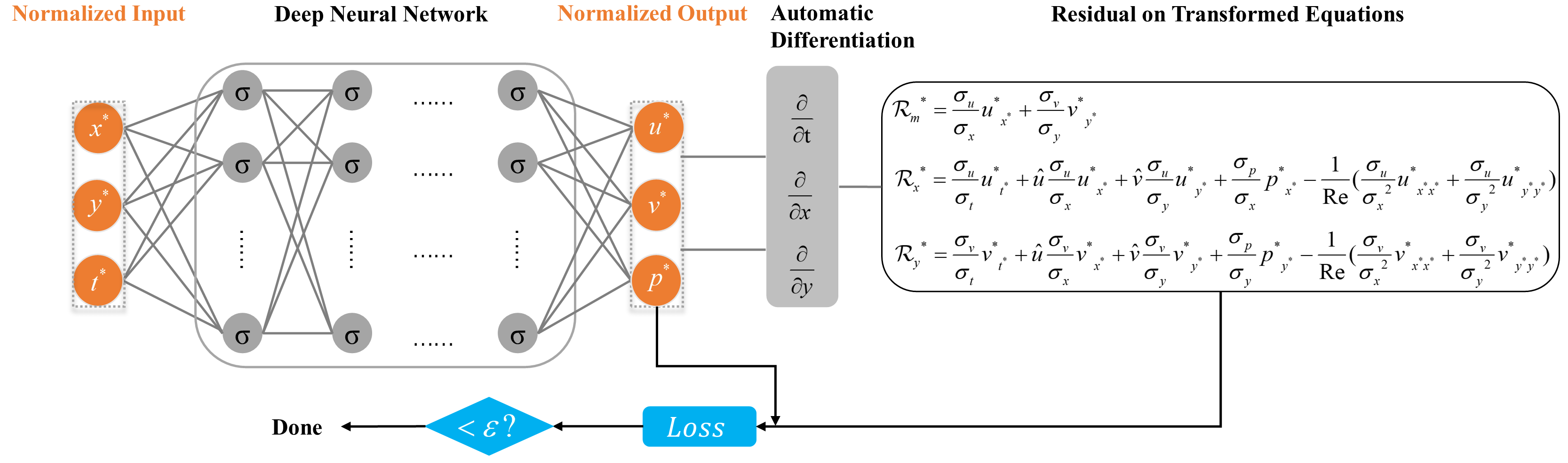
Figure 3: Normalized PINNs for solving non-dimensional equations. Both the input and output variables are normalized using mean values and standard deviation values. The loss function consists of both the normalized data loss and the residual error of the transformed equations.

$$\Psi={\sigma_{\Psi}}\odot({\Psi^{*}}+\bar{\Psi})$$ (12)

where $\odot$ means the element-wise product.

III Numerical Dataset Used for Training and Validation

In this paper, three open source turbulent flow cases at different Reynolds numbers ($Re$) were examined to evaluate the performance of the proposed preprocessing pipeline in reconstructing flow fields, i.e. the wake flow past a 2-dimensional (2D) circular cylinder at $Re=3900$ (simulated with $k-\epsilon$ model), 2D decaying turbulence at $Re=2000$Xu et al. (2023b) (simulated with pseudo-spectral methodLauber (2021)), and the wake flow past a 2D circular cylinder at $Re=10000$Yan et al. (2023) (simulated with $k-\omega sst$ model).

The data used in flow field reconstruction is typically sparse in spatial domain and dense in temporal domain, simulating the realistic experiment set up. Taking the cylinder wake flow at Reynolds number ${Re}=3900$ case as an example, the sparse flow data ${u,v,p}$ is sampled from 36 sparsely distributed points covering a period of 42.9 seconds, as shown in Fig.4. The total number of data points $N_{d}$ is 3600, with 36 data points in each of the 100 snapshots. The overall number of residual points $N_{r}$ is 1000000, sampled through Latin Hypercube Sampling (LHS) method in the normalized spatio-temporal domain. The training sets for all three cases are similar, as presented in Table.1

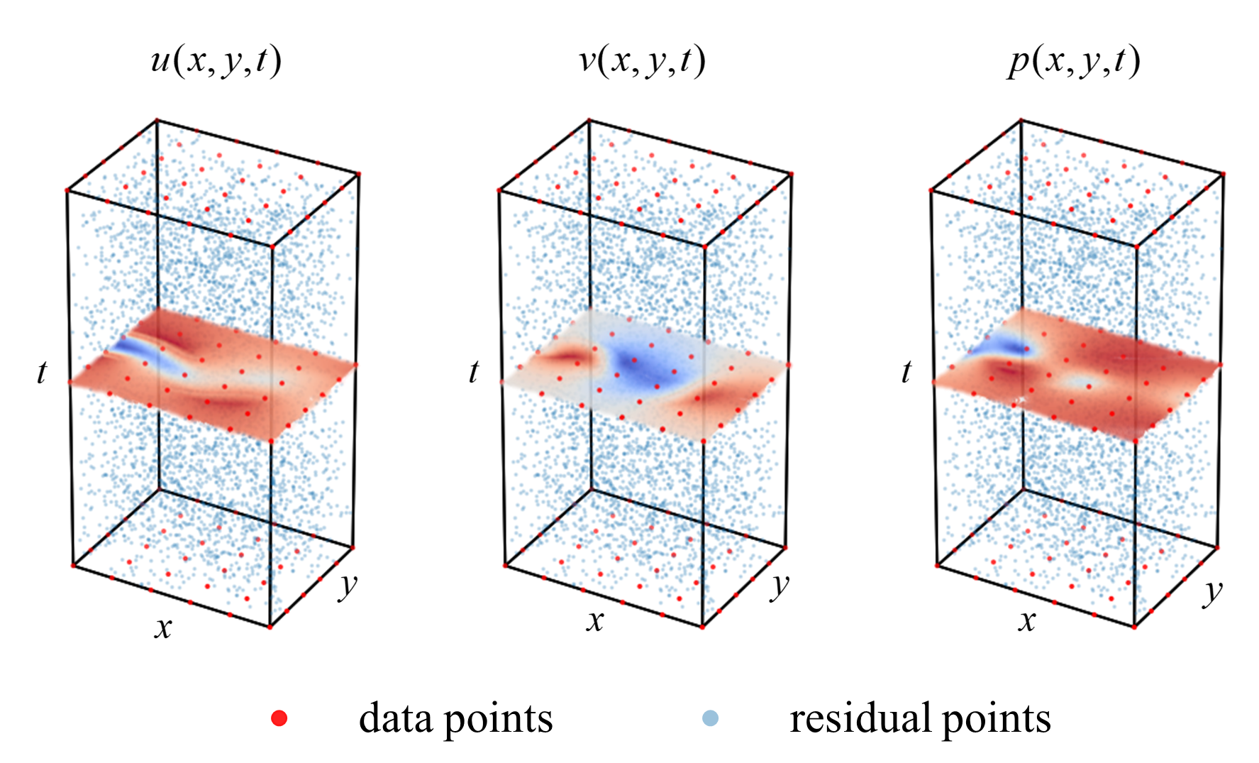
Figure 4: Schematic of sparse reconstruction training set for the wake flow of 2D cylinder. Left: stream-wise velocity $u$. Middle: transverse velocity $v$. Right: pressure $p$. 36 sparsely distributed data points from 100 snapshots (only 3 snapshots are plotted) covering a period of 42.9 seconds are taken as training dataset, along with 1000000 residual points sampled through Latin Hypercube Sampling.

Table 1: Training set information for flow reconstruction cases.

Case	$Re$	Data points	Snapshots/ Duration	Residual points
cylinder wake	3900	3600	100/42.9s	1000000
	10000	3600	100/2.86s	1000000
decaying turbulence	2000	3600	100/1.3s	1000000

More detailed information and verification about these three cases can be referenced in literature 32 and 51. The original dataset can be found in PINN-MPI and PINN-POD.

IV Results

In this section, the qualitative reconstruction results of three turbulent flow cases are demonstrated with contour plots and pointwise error. The quantitative results of the proposed normalization method are compared with the results of the baseline method (without normalization) and the inner normalization layer method through relative $L_{2}$ norm, as defined in Eq.13.

$${R_{L_{2}}}=\frac{{\left\|{\hat{U}-U}\right\|}}{{\left\|U\right\|}}$$ (13)

Where ${\left\|U\right\|}$ denotes the $L_{2}$ norm of original benchmark data and ${\left\|{\hat{U}-U}\right\|}$ denotes the $L_{2}$ norm of the deviation between PINNs prediction and benchmark data. Since the problem scales are similar for all three cases, to effectively showcase the impact of normalization, identical training hyperparameters are used for all cases and methods, as detailed in Table 2.

Table 2: Hyperparameters for PINNs.

Hyperparameters	Meaning	Value
$L_{h}$	Number of hidden layers	10
$N_{h}$	Neurons per hidden layer	32
$l_{r0}$	Initial learning rate	1e-3
$schedule$	Learning rate schedule	exp
$\gamma$	Exponential rate of learning schedule	0.999
$\sigma$	Activation function	tanh
$epochs$	Number of training epochs	5000
$batchsize$	Number of residual points in one batch	10000
$optimizer$	Algorithm for minimizing loss function	AdamKingma and Ba (2014)
$\lambda_{r}$	Weight of residual loss	1

Previous research indicates that PINNs perform better with a decreasing learning rate. Therefore the specific learning rate schedule adopted in this paper is exponential learning rate (referred to as "exp" in Table.2), as given by Eq.14. Following each batch training of residual points, all data points are trained once to enhance the alignment of PINNs’ predictions with the sparse data provided. All training sessions were performed on the NVIDIA GeForce RTX 3060 GPU, with a similar training time of 4.5 seconds per epoch.

$${l_{r}}={l_{r0}}*{\gamma^{epoch}}$$ (14)

IV.1 Cylinder wake at Re=3900

Through incorporating non-dimensional equations, the original flow field of wake flow past a 2D circular cylinder at $Re=3900$ covering the spatiotemporal domain $x\in[1.000,5.000],y\in[-2.000,2.000],t\in[0.000,42.937]$ can be successfully reconstructed from 36 sparsely distributed measurements, as shown in the second column of Fig.5. The correctness of the proposed normalization method can be verified by the contour plot displayed in the third column of Fig.5. The high consistency between the reconstructed velocity and pressure (using normalization method) and the benchmark numerical data proves the normalization on data and the transformation on non-dimensional equations are valid. The pointwise error comparison between the fourth and fifth column of Fig.5 qualitatively illustrates not only the validity but also the superiority of the proposed method. By employing the normalization method, the errors of stream-wise velocity $u$, transverse velocity $v$, and pressure $p$ are all lower than those predicted by the baseline method of simply incorporating the non-dimensional equations.

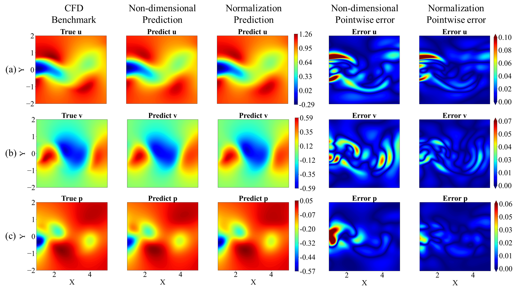
Figure 5: Flow past 2D circular cylinder at Re=3900. CFD benchmark flow field (first column), predicted flow field using non-dimensional equations (second column) and normalization method (third column), and the pointwise error between benchmark field and predicted field using non-dimensional equations (fourth column) and normalization method (fifth column) at the time snapshot $t=38.17$. (a): stream-wise velocity $u$; (b): transverse velocity $v$; (c): pressure $p$.

Furthermore, to quantitatively compare the proposed normalization method with current methods and to eliminate the influence of randomness, 5 independent runs of training were performed for each method and the relative $L_{2}$ norms between benchmark flow field and PINNs predictions were calculated and averaged. As shown in Fig.6, after 5000 epochs of training, the obtained average relative $L_{2}$ norms of $u,v,p$ using normalization method are 0.0188, 0.0331 and 0.0471, which are 34% to 46% lower than 0.0285, 0.0569 and 0.0881 obtained using non-dimensional equations alone. The corresponding values obtained using inner normalization method are 0.0275, 0.0538, 0.0855, only slightly better than solely applying non-dimensional equations. Moreover, the normalization method provides the best prediction on all three flow quantities during the entire training process, which is probably resulted from the more concentrated data range after normalization. Fig.7 further gives a detailed comparison of average relative $L_{2}$ norms at each time snapshot after 5000 epochs of training: while the inner normalization layer method exhibits similar prediction accuracy to that of using non-dimensional equations, the proposed normalization method demonstrates a significantly enhanced prediction accuracy of $u,v,p$ at each time snapshot, underscoring the effectiveness of real normalization.

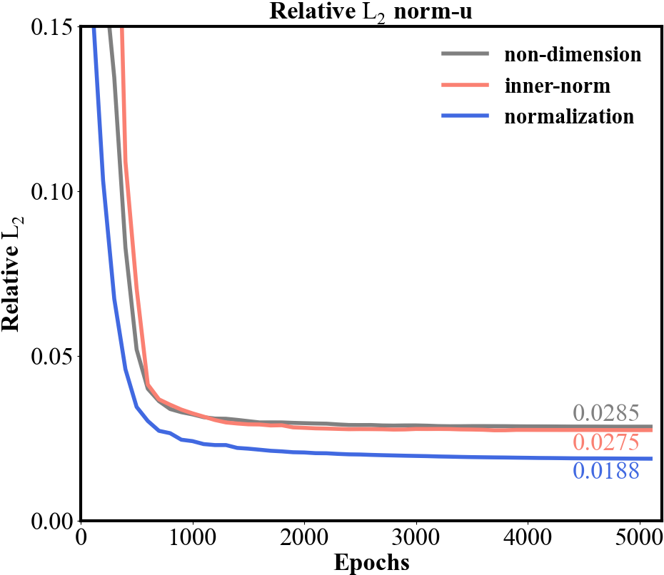
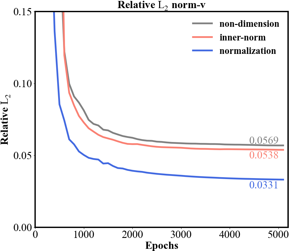
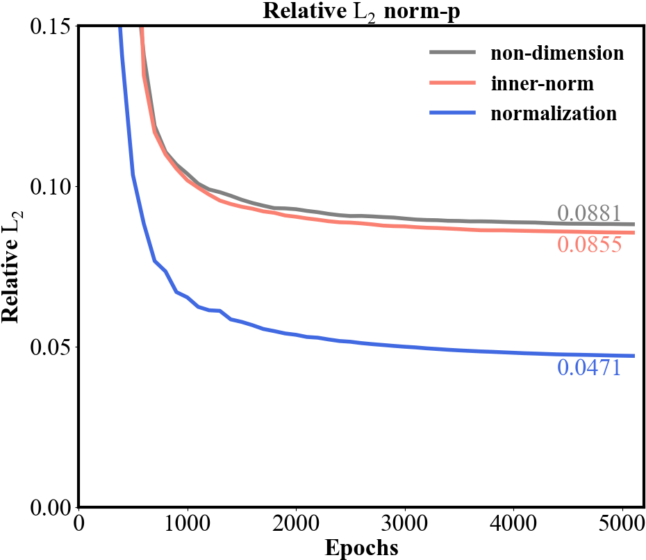
Figure 6: Relative $L_{2}$ norms while training. The relative $L_{2}$ norms of (a): stream-wise velocity $u$, (b): transverse velocity $v$, (c): pressure $p$ between benchmark flow data (flow past 2D circular cylinder at Re=3900) and predicted flow data using non-dimensional equations, inner normalization layer method and normalization method. The relative L2 norms are averaged values calculated from five independent runs.

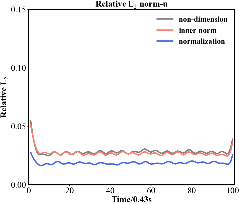
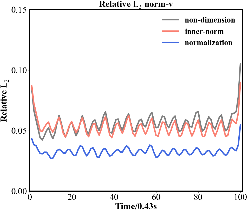
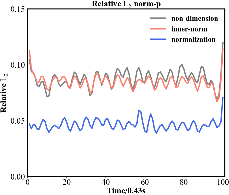
Figure 7: Relative $L_{2}$ norms for each time snapshot after training. The relative $L_{2}$ norms of (a): stream-wise velocity $u$, (b): transverse velocity $v$, (c): pressure $p$ between benchmark flow data (flow past 2D circular cylinder at Re=3900) and predicted flow data using non-dimensional equations, inner normalization layer method and normalization method. The relative L2 norms are averaged values calculated from five independent runs.

IV.2 Cylinder wake at Re=10000

Subsequently, the flow field of wake flow past a 2D circular cylinder at $Re=10000$ was also reconstructed to assess the efficacy of the proposed normalization method. Covering the spatiotemporal domain $x\in[1.000,5.000],y\in[-2.000,2.000],t\in[0.000,2.863]$, the cylinder wake can also be satisfyingly reconstructed from 36 sparsely distributed measurements through simply incorporating non-dimensional equations, as depicted in the second column of Fig.8. The contour plot in the third column of Fig.8 once again confirms the correctness of the normalization method, despite the different Reynolds numbers and different turbulence models used in generating the numerical datasets.

Qualitatively, the pointwise error of normalization method is noticeably smaller than that of not applying normalization, as illustrated in the fourth and fifth column of Fig.8. Quantitatively, as depicted in Fig.9, the average relative $L_{2}$ norms of transverse velocity $v$ and pressure $p$ are almost indistinguishable between adopting inner normalization layer method and simply using non-dimensional equations (0.0365 compared to 0.0359 for $v$, and 0.0373 compared to 0.0372 for $p$), and the average relative $L_{2}$ norm of stream-wise velocity $u$ obtained by inner normalization layer method is even slightly higher (0.0183 compared to 0.0181). In comparison, our proposed normalization method presents a robustly higher prediction accuracy for all three flow quantities throughout the training process. Following 5000 training epochs, the final average relative $L_{2}$ norms of $u,v,p$ obtained using normalization method are 0.0137, 0.0281 and 0.0273, representing approximately a 25% improvement compared to the values obtained using non-dimensional equations. Further, looking closer at each time snapshot, while the average relative $L_{2}$ norm curves obtained using inner normalization layer method are overlapped with and sometimes even worse than the curves obtained using non-dimensional equations, the average relative $L_{2}$ norm curves obtained using normalization method are distinctly better than the other two methods at every snapshot, as illustrated in Fig.10.

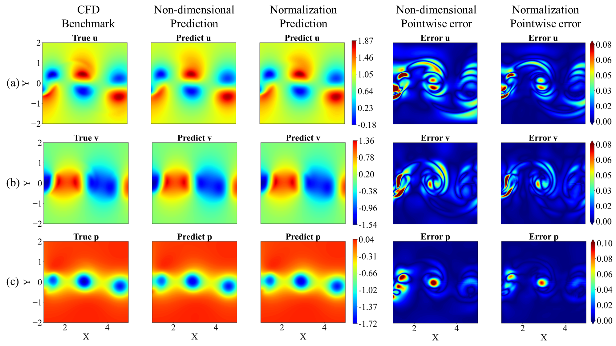
Figure 8: Flow past 2D circular cylinder at Re=10000. CFD benchmark flow field (first column), predicted flow field using non-dimensional equations (second column) and normalization method (third column), and the pointwise error between benchmark field and predicted field using non-dimensional equations (fourth column) and normalization method (fifth column) at the time snapshot $t=0.58$. (a): stream-wise velocity $u$; (b): transverse velocity $v$; (c): pressure $p$.

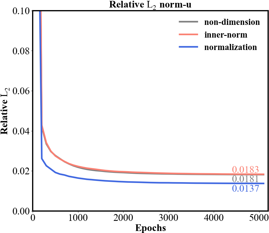
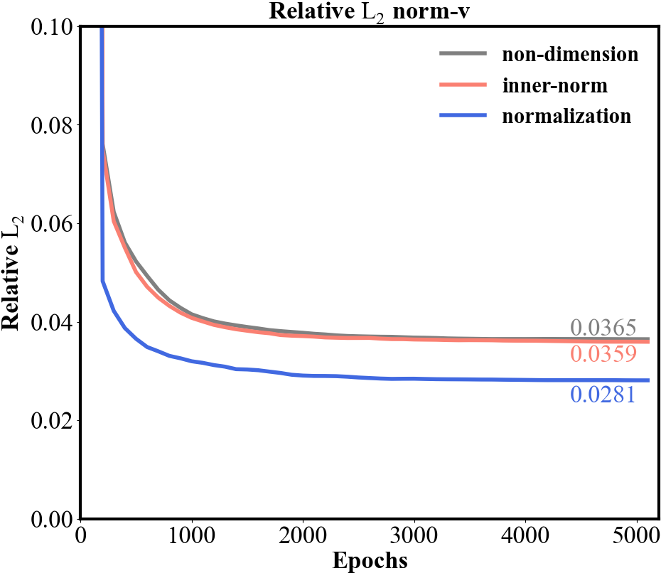
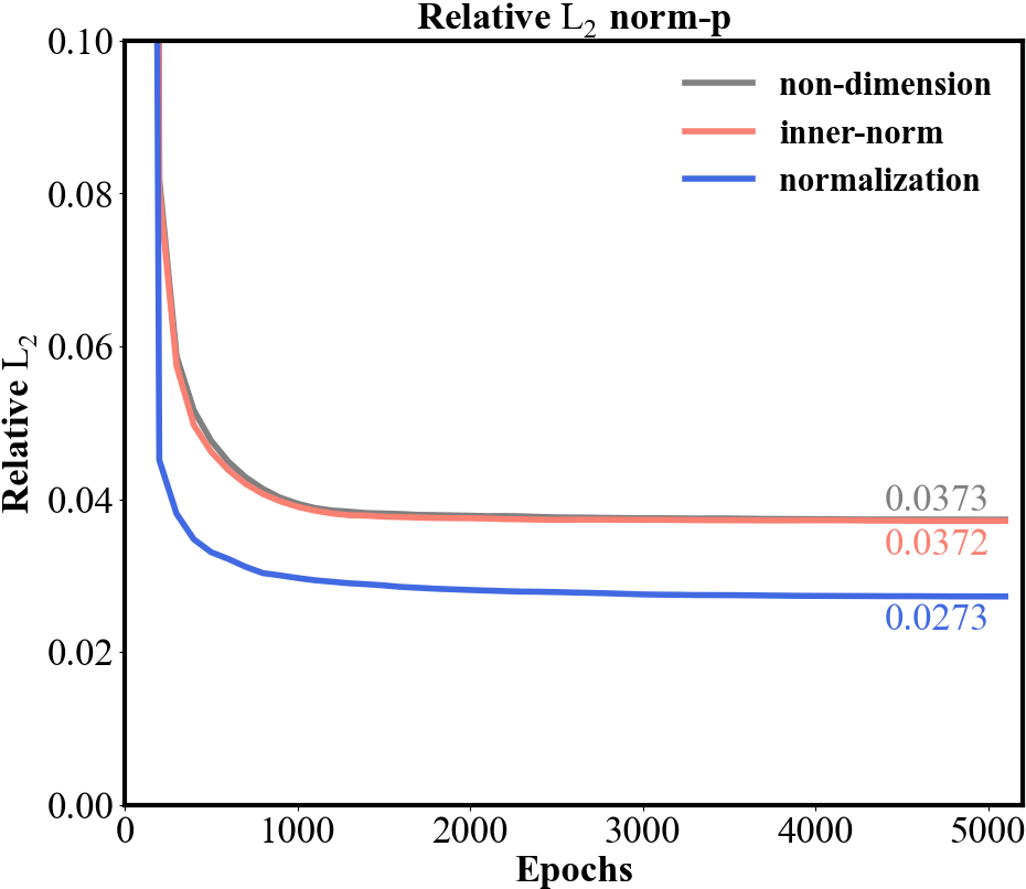
Figure 9: Relative $L_{2}$ norms while training. The relative $L_{2}$ norms of (a): stream-wise velocity $u$, (b): transverse velocity $v$, (c): pressure $p$ between benchmark flow data (flow past 2D circular cylinder at Re=10000) and predicted flow data using non-dimensional equations, inner normalization layer method and normalization method. The relative L2 norms are averaged values calculated from five independent runs.

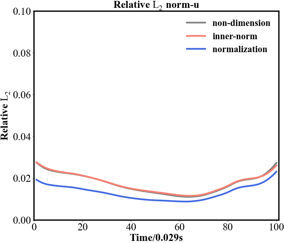
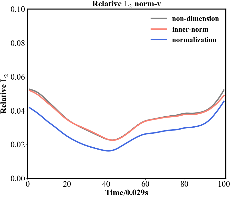
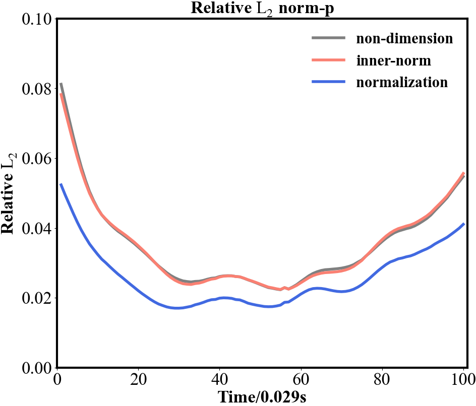
Figure 10: Relative $L_{2}$ norms for each time snapshot after training. The relative $L_{2}$ norms of (a): stream-wise velocity $u$, (b): transverse velocity $v$, (c): pressure $p$ between benchmark flow data (flow past 2D circular cylinder at Re=10000) and predicted flow data using non-dimensional equations, inner normalization layer method and normalization method. The relative L2 norms are averaged values calculated from five independent runs.

IV.3 Decaying turbulence at Re=2000

Finally, 36 sparse measurements covering the spatiotemporal domain $x\in[0.50\pi,1.50\pi],y\in[0.50\pi,1.50\pi],t\in[19.637,20.935]$ of 2D decaying turbulence at $Re=2000$ were utilized to reconstruct the flow field. Similar to previous two cases, for the reconstruction of all three flow quantities, the proposed normalization method is qualitatively better than the baseline method of simply applying non-dimensional equations, as demonstrated in the fourth and fifth column of Fig.11.

Quantitatively, the final average relative $L_{2}$ norms of $u,v,p$ obtained using normalization method are 0.0319, 0.0213 and 0.0079, which are 20%, 16%, and 10% lower than the relative $L_{2}$ norms obtained using baseline method, as depicted in Fig.12. Given the narrower data range in this case and the relatively accurate prediction of pressure values themselves, the proposed method does not exhibit as prominent advantages in this case as in the previous two. Nonetheless, the normalization method still presents the best prediction for all three flow quantities throughput the training process, without increasing the computational cost. Notably, though the inner normalization layer method does demonstrate relatively good improvement in prediction accuracy of all three quantities in this case, for the closer examination of average relative $L_{2}$ norms in each time snapshot, it can be found in Fig.13 that the prediction accuracy of inner normalization layer method becomes inferior to the baseline method of applying non-dimensional equations. Contrarily, albeit occasionally marginal, the average relative $L_{2}$ norms obtained using normalization method are consistently lower than those obtained by baseline method for every snapshot, demonstrating its superiority.

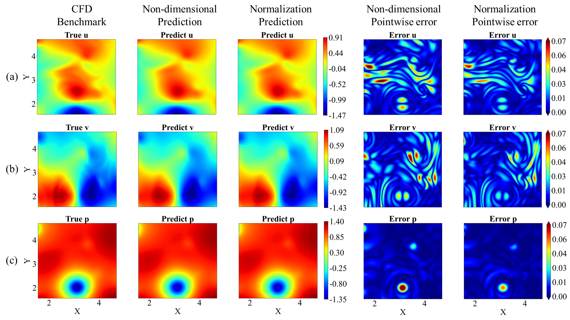
Figure 11: Decaying turbulence at Re=2000. CFD benchmark flow field (first column), predicted flow field using non-dimensional equations (second column) and normalization method (third column), and the pointwise error between benchmark field and predicted field using non-dimensional equations (fourth column) and normalization method (fifth column) at the time snapshot $t=19.90$. (a): stream-wise velocity $u$; (b): transverse velocity $v$; (c): pressure $p$.

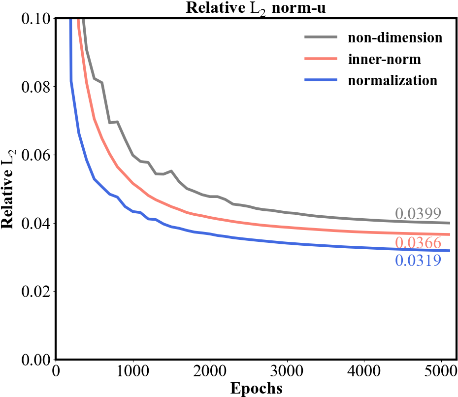
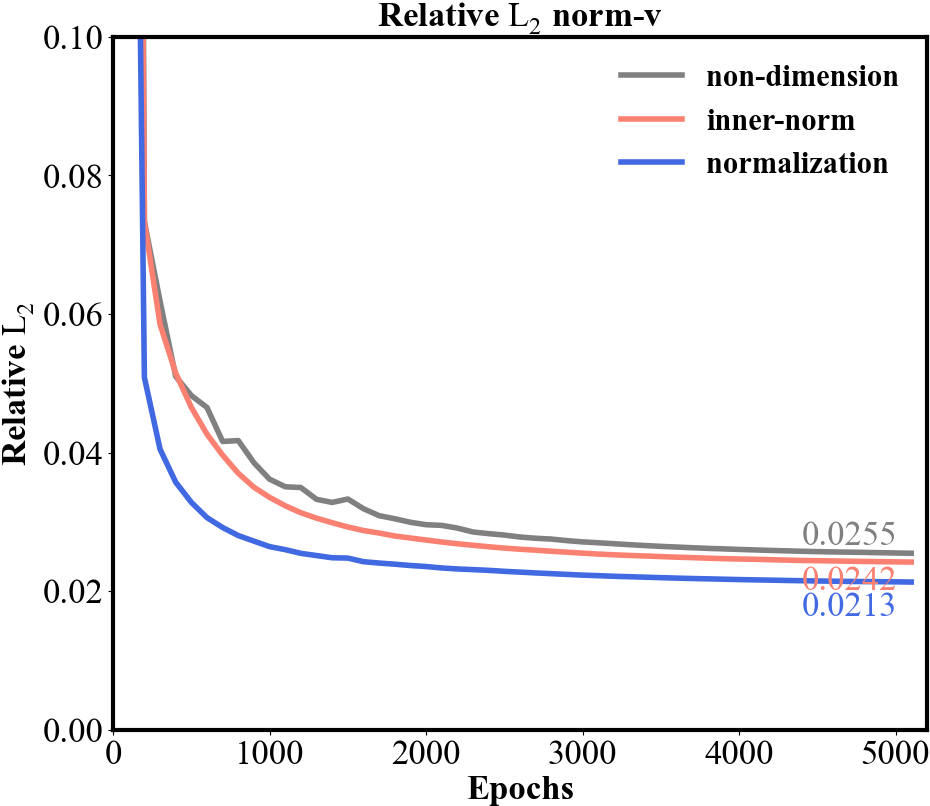
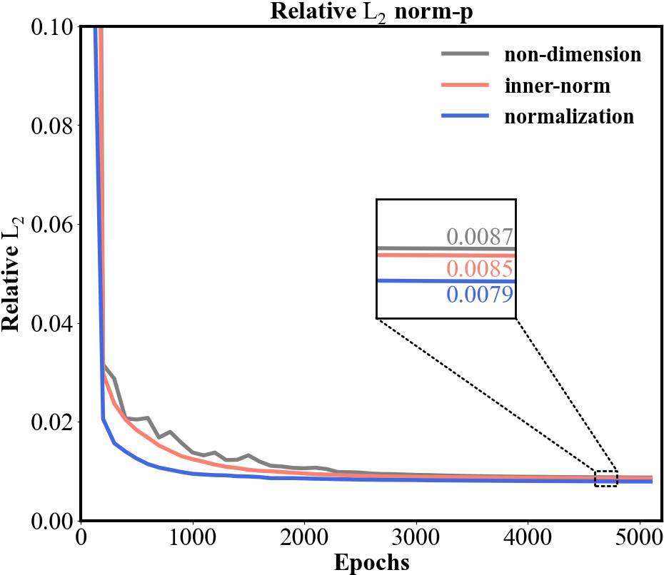
Figure 12: Relative $L_{2}$ norms while training. The relative $L_{2}$ norms of (a): stream-wise velocity $u$, (b): transverse velocity $v$, (c): pressure $p$ between benchmark flow data (decaying turbulence at Re=2000) and predicted flow data using non-dimensional equations, inner normalization layer method and normalization method. The relative L2 norms are averaged values calculated from five independent runs.

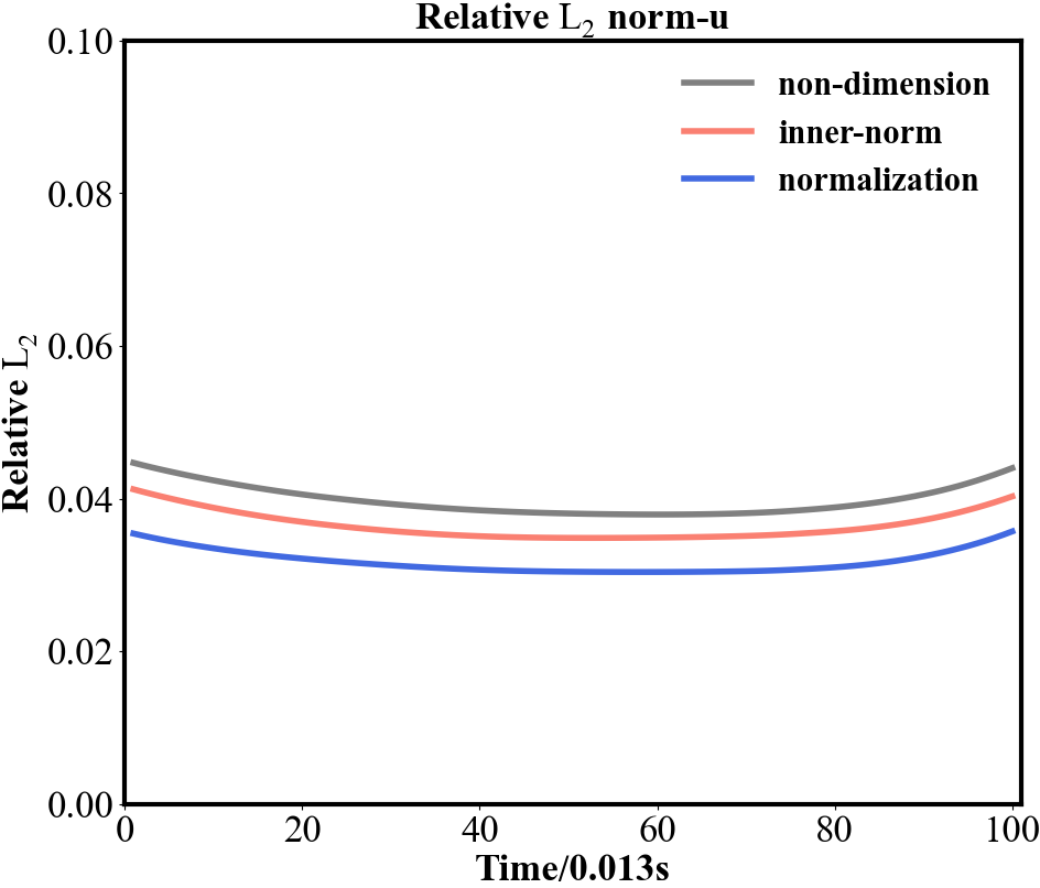
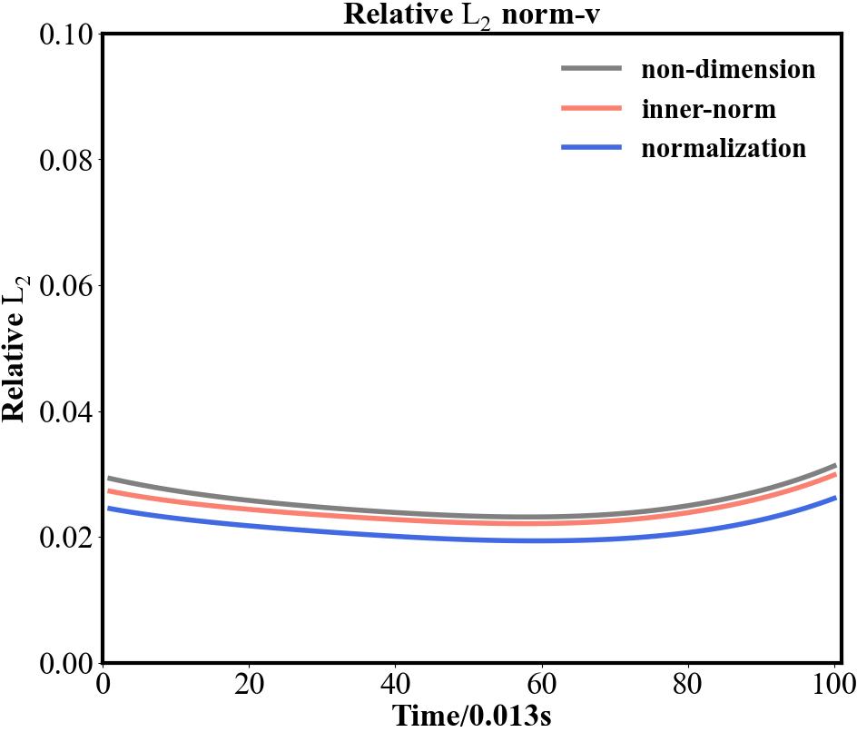
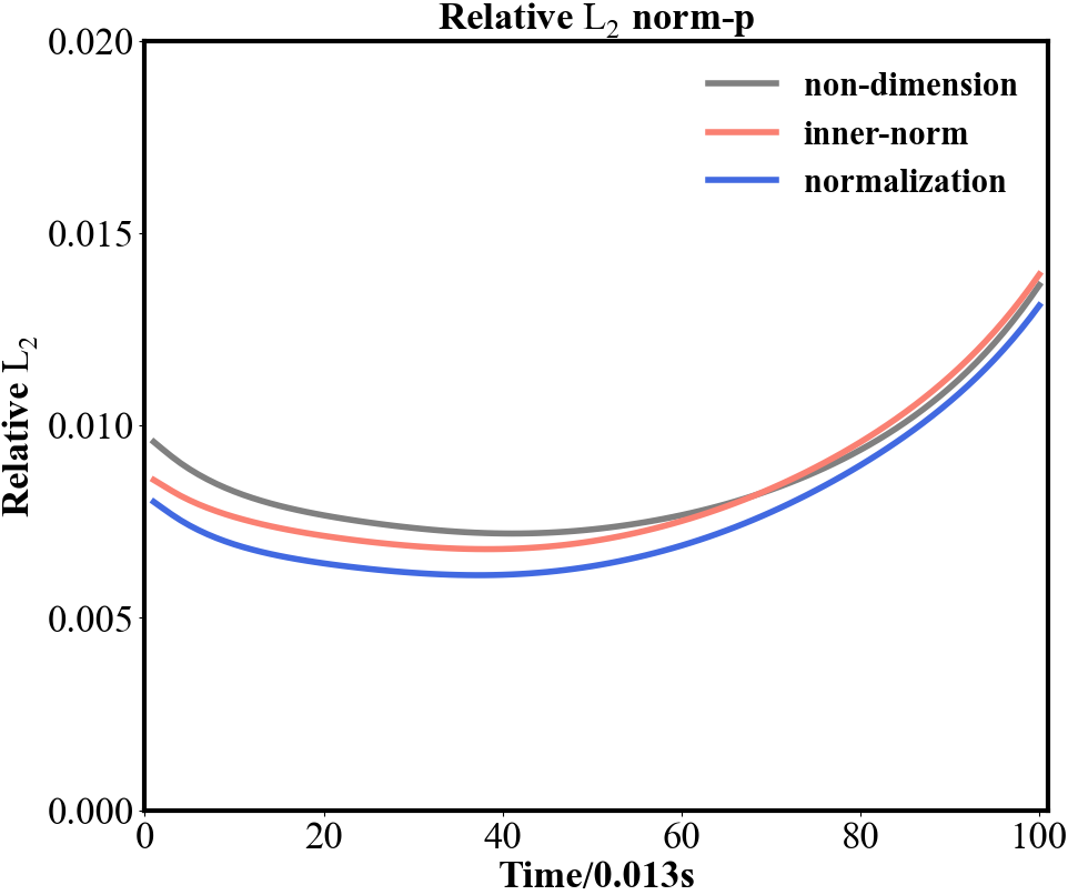
Figure 13: Relative $L_{2}$ norms for each time snapshot after training. The relative $L_{2}$ norms of (a): stream-wise velocity $u$, (b): transverse velocity $v$, (c): pressure $p$ between benchmark flow data (decaying turbulence at Re=2000) and predicted flow data using non-dimensional equations, inner normalization layer method and normalization method. The relative L2 norms are averaged values calculated from five independent runs.

V Conclusion and discussion

To summarize, we proposed a data preprocessing method for Physics-informed Neural networks, with a specific focus on data normalization. Unlike the expedient approach of adding an inner normalization layer, our normalization method involves directly normalizing both input and output data. The neural networks are then constructed using these normalized features, aligning with the prevalent data normalization techniques in classic machine learning. By concurrently normalizing the data and transforming the corresponding equations, the inverse problem of flow field reconstruction was better solved than simply applying non-dimensional equations or adding an extra inner normalization layer. In the context of three turbulent flow cases - the wake flow past 2D circular cylinder at $Re=3900$, the wake flow past 2D circular cylinder at $Re=10000$, and 2D decaying turbulence at $Re=2000$, the proposed normalization method consistently yield lower relative $L_{2}$ norm values for each flow variable $u,v,p$, showing reductions from 10% to 46%. This improvement was achieved despite the variations in Reynolds numbers and turbulence models used in the simulations. Moreover, for the unsteady reconstruction, the relative $L_{2}$ norms obtained using normalization method were consistently lower than those obtained using baseline method (only applying non-dimensional equations) in every time snapshot. While the intuitive-based inner normalization layer method exhibited some enhancement in prediction accuracy for the three tested cases, the gains were marginal and often negligible, with some cases demonstrating worsened performance when compared to the baseline method of solely applying non-dimensional equations. On the contrary, the intuitive-and-mathematical-based normalization method exhibited much more prominent advantage in predicting all flow quantities, highlighting its validity and superiority. Despite utilizing only 36 sparsely distributed data points, the mean and standard deviation values derived from this limited dataset effectively showcased the method’s ability to optimize data utilization, hinting at its potential applicability for larger datasets in inverse problems.

While the present study solely validated the normalization method on the 2D unsteady NS equations, the underlying mathematical principles of the calculus technique employed to transform these equations are universally applicable to all types of differential equations. Whether dealing with dimensional or non-dimensional equations, ordinary or partial differential equations, they can all undergo normalization using a consistent preprocessing approach. We actively anticipate widespread adoption of the proposed normalization method across diverse types of differential equations, potentially establishing itself as an essential preprocessing technique for training PINNs.

Data Availability Statement

The data and code that support the findings of this study will soon be available on https://github.com/Shengfeng233/PINN-Preprocess.

References

- Kiran et al. (2021) B. R. Kiran, I. Sobh, V. Talpaert, P. Mannion, A. A. Al Sallab, S. Yogamani, and P. Pérez, “Deep reinforcement learning for autonomous driving: A survey,” IEEE Transactions on Intelligent Transportation Systems 23, 4909–4926 (2021).
- Portugal, Alencar, and Cowan (2018) I. Portugal, P. Alencar, and D. Cowan, “The use of machine learning algorithms in recommender systems: A systematic review,” Expert Systems with Applications 97, 205–227 (2018).
- Morgan and Jacobs (2020) D. Morgan and R. Jacobs, “Opportunities and challenges for machine learning in materials science,” Annual Review of Materials Research 50, 71–103 (2020).
- Greener et al. (2022) J. G. Greener, S. M. Kandathil, L. Moffat, and D. T. Jones, “A guide to machine learning for biologists,” Nature Reviews Molecular Cell Biology 23, 40–55 (2022).
- Brunton, Noack, and Koumoutsakos (2020) S. L. Brunton, B. R. Noack, and P. Koumoutsakos, “Machine learning for fluid mechanics,” Annual review of fluid mechanics 52, 477–508 (2020).
- Karniadakis et al. (2021) G. E. Karniadakis, I. G. Kevrekidis, L. Lu, P. Perdikaris, S. Wang, and L. Yang, “Physics-informed machine learning,” Nature Reviews Physics 3, 422–440 (2021).
- Cuomo et al. (2022) S. Cuomo, V. S. Di Cola, F. Giampaolo, G. Rozza, M. Raissi, and F. Piccialli, “Scientific machine learning through physics–informed neural networks: where we are and what’s next,” Journal of Scientific Computing 92, 88 (2022).
- Lagaris, Likas, and Fotiadis (1998) I. E. Lagaris, A. Likas, and D. I. Fotiadis, “Artificial neural networks for solving ordinary and partial differential equations,” IEEE transactions on neural networks 9, 987–1000 (1998).
- Raissi, Perdikaris, and Karniadakis (2019) M. Raissi, P. Perdikaris, and G. E. Karniadakis, “Physics-informed neural networks: A deep learning framework for solving forward and inverse problems involving nonlinear partial differential equations,” Journal of Computational physics 378, 686–707 (2019).
- Yang, Meng, and Karniadakis (2021) L. Yang, X. Meng, and G. E. Karniadakis, “B-pinns: Bayesian physics-informed neural networks for forward and inverse pde problems with noisy data,” Journal of Computational Physics 425, 109913 (2021).
- Yu et al. (2022) J. Yu, L. Lu, X. Meng, and G. E. Karniadakis, “Gradient-enhanced physics-informed neural networks for forward and inverse pde problems,” Computer Methods in Applied Mechanics and Engineering 393, 114823 (2022).
- Zhang et al. (2023) Z.-Y. Zhang, H. Zhang, L.-S. Zhang, and L.-L. Guo, “Enforcing continuous symmetries in physics-informed neural network for solving forward and inverse problems of partial differential equations,” Journal of Computational Physics 492, 112415 (2023).
- Cai et al. (2021a) S. Cai, Z. Wang, S. Wang, P. Perdikaris, and G. E. Karniadakis, “Physics-informed neural networks for heat transfer problems,” Journal of Heat Transfer 143 (2021a).
- Jagtap, Mudunuru, and Nakshatrala (2023) N. V. Jagtap, M. Mudunuru, and K. Nakshatrala, “Coolpinns: A physics-informed neural network modeling of active cooling in vascular systems,” Applied Mathematical Modelling 122, 265–287 (2023).
- Ren et al. (2024) P. Ren, C. Rao, S. Chen, J.-X. Wang, H. Sun, and Y. Liu, “Seismicnet: Physics-informed neural networks for seismic wave modeling in semi-infinite domain,” Computer Physics Communications 295, 109010 (2024).
- Zhou and Yan (2021) Z. Zhou and Z. Yan, “Solving forward and inverse problems of the logarithmic nonlinear schrödinger equation with pt-symmetric harmonic potential via deep learning,” Physics Letters A 387, 127010 (2021).
- Jin, Mattheakis, and Protopapas (2022) H. Jin, M. Mattheakis, and P. Protopapas, “Physics-informed neural networks for quantum eigenvalue problems,” in 2022 International Joint Conference on Neural Networks (IJCNN) (IEEE, 2022) pp. 1–8.
- Cai et al. (2021b) S. Cai, Z. Mao, Z. Wang, M. Yin, and G. E. Karniadakis, “Physics-informed neural networks (pinns) for fluid mechanics: A review,” Acta Mechanica Sinica 37, 1727–1738 (2021b).
- Sharma et al. (2023) P. Sharma, W. T. Chung, B. Akoush, and M. Ihme, “A review of physics-informed machine learning in fluid mechanics,” Energies 16, 2343 (2023).
- Rao, Sun, and Liu (2020) C. Rao, H. Sun, and Y. Liu, “Physics-informed deep learning for incompressible laminar flows,” Theoretical and Applied Mechanics Letters 10, 207–212 (2020).
- Biswas and Anand (2023) S. K. Biswas and N. Anand, “Three-dimensional laminar flow using physics informed deep neural networks,” Physics of Fluids 35 (2023).
- Jin et al. (2021) X. Jin, S. Cai, H. Li, and G. E. Karniadakis, “Nsfnets (navier-stokes flow nets): Physics-informed neural networks for the incompressible navier-stokes equations,” Journal of Computational Physics 426, 109951 (2021).
- Hanrahan, Kozul, and Sandberg (2023) S. Hanrahan, M. Kozul, and R. Sandberg, “Studying turbulent flows with physics-informed neural networks and sparse data,” International Journal of Heat and Fluid Flow 104, 109232 (2023).
- Raissi, Yazdani, and Karniadakis (2020) M. Raissi, A. Yazdani, and G. E. Karniadakis, “Hidden fluid mechanics: Learning velocity and pressure fields from flow visualizations,” Science 367, 1026–1030 (2020).
- Cai et al. (2021c) S. Cai, Z. Wang, F. Fuest, Y. J. Jeon, C. Gray, and G. E. Karniadakis, “Flow over an espresso cup: inferring 3-d velocity and pressure fields from tomographic background oriented schlieren via physics-informed neural networks,” Journal of Fluid Mechanics 915, A102 (2021c).
- Fathi et al. (2020) M. F. Fathi, I. Perez-Raya, A. Baghaie, P. Berg, G. Janiga, A. Arzani, and R. M. D’Souza, “Super-resolution and denoising of 4d-flow mri using physics-informed deep neural nets,” Computer Methods and Programs in Biomedicine 197, 105729 (2020).
- Baydin et al. (2018) A. G. Baydin, B. A. Pearlmutter, A. A. Radul, and J. M. Siskind, “Automatic differentiation in machine learning: a survey,” Journal of Marchine Learning Research 18, 1–43 (2018).
- Sun et al. (2020) L. Sun, H. Gao, S. Pan, and J.-X. Wang, “Surrogate modeling for fluid flows based on physics-constrained deep learning without simulation data,” Computer Methods in Applied Mechanics and Engineering 361, 112732 (2020).
- Xu et al. (2023a) S. Xu, Z. Sun, R. Huang, D. Guo, G. Yang, and S. Ju, “A practical approach to flow field reconstruction with sparse or incomplete data through physics informed neural network,” Acta Mechanica Sinica 39, 1–15 (2023a).
- Xu, Zhang, and Wang (2021) H. Xu, W. Zhang, and Y. Wang, “Explore missing flow dynamics by physics-informed deep learning: The parameterized governing systems,” Physics of Fluids 33, 095116 (2021).
- Wang et al. (2024) L. Wang, M. Chen, Z. Luo, B. Zhang, J. Xu, Z. Wang, and A. C. Tan, “Dynamic wake field reconstruction of wind turbine through physics-informed neural network and sparse lidar data,” Energy , 130401 (2024).
- Xu et al. (2023b) S. Xu, C. Yan, G. Zhang, Z. Sun, R. Huang, S. Ju, D. Guo, and G. Yang, “Spatiotemporal parallel physics-informed neural networks: A framework to solve inverse problems in fluid mechanics,” Physics of Fluids 35 (2023b).
- Liu et al. (2024) S. Liu, H. Wang, J. H. Chen, K. Luo, and J. Fan, “High-resolution reconstruction of turbulent flames from sparse data with physics-informed neural networks,” Combustion and Flame 260, 113275 (2024).
- Jagtap, Kharazmi, and Karniadakis (2020) A. D. Jagtap, E. Kharazmi, and G. E. Karniadakis, “Conservative physics-informed neural networks on discrete domains for conservation laws: Applications to forward and inverse problems,” Computer Methods in Applied Mechanics and Engineering 365, 113028 (2020).
- Hu et al. (2023) Z. Hu, A. D. Jagtap, G. E. Karniadakis, and K. Kawaguchi, “Augmented physics-informed neural networks (apinns): A gating network-based soft domain decomposition methodology,” Engineering Applications of Artificial Intelligence 126, 107183 (2023).
- Meng et al. (2020) X. Meng, Z. Li, D. Zhang, and G. E. Karniadakis, “Ppinn: Parareal physics-informed neural network for time-dependent pdes,” Computer Methods in Applied Mechanics and Engineering 370, 113250 (2020).
- Wang, Sankaran, and Perdikaris (2024) S. Wang, S. Sankaran, and P. Perdikaris, “Respecting causality for training physics-informed neural networks,” Computer Methods in Applied Mechanics and Engineering 421, 116813 (2024).
- Chiu et al. (2022) P.-H. Chiu, J. C. Wong, C. Ooi, M. H. Dao, and Y.-S. Ong, “Can-pinn: A fast physics-informed neural network based on coupled-automatic–numerical differentiation method,” Computer Methods in Applied Mechanics and Engineering 395, 114909 (2022).
- Costabal, Pezzuto, and Perdikaris (2024) F. S. Costabal, S. Pezzuto, and P. Perdikaris, “-pinns: physics-informed neural networks on complex geometries,” Engineering Applications of Artificial Intelligence 127, 107324 (2024).
- Jagtap, Kawaguchi, and Em Karniadakis (2020) A. D. Jagtap, K. Kawaguchi, and G. Em Karniadakis, “Locally adaptive activation functions with slope recovery for deep and physics-informed neural networks,” Proceedings of the Royal Society A 476, 20200334 (2020).
- Jagtap, Kawaguchi, and Karniadakis (2020) A. D. Jagtap, K. Kawaguchi, and G. E. Karniadakis, “Adaptive activation functions accelerate convergence in deep and physics-informed neural networks,” Journal of Computational Physics 404, 109136 (2020).
- McClenny and Braga-Neto (2023) L. D. McClenny and U. M. Braga-Neto, “Self-adaptive physics-informed neural networks,” Journal of Computational Physics 474, 111722 (2023).
- Xu et al. (2023c) C. Xu, B. T. Cao, Y. Yuan, and G. Meschke, “Transfer learning based physics-informed neural networks for solving inverse problems in engineering structures under different loading scenarios,” Computer Methods in Applied Mechanics and Engineering 405, 115852 (2023c).
- García, Luengo, and Herrera (2015) S. García, J. Luengo, and F. Herrera, Data preprocessing in data mining, Vol. 72 (Springer, 2015).
- Kotsiantis, Kanellopoulos, and Pintelas (2006) S. B. Kotsiantis, D. Kanellopoulos, and P. E. Pintelas, “Data preprocessing for supervised leaning,” International journal of computer science 1, 111–117 (2006).
- García et al. (2016) S. García, S. Ramírez-Gallego, J. Luengo, J. M. Benítez, and F. Herrera, “Big data preprocessing: methods and prospects,” Big Data Analytics 1, 1–22 (2016).
- De Florio et al. (2024) M. De Florio, E. Schiassi, F. Calabrò, and R. Furfaro, “Physics-informed neural networks for 2nd order odes with sharp gradients,” Journal of Computational and Applied Mathematics 436, 115396 (2024).
- Mishra and Molinaro (2023) S. Mishra and R. Molinaro, “Estimates on the generalization error of physics-informed neural networks for approximating pdes,” IMA Journal of Numerical Analysis 43, 1–43 (2023).
- Maddu et al. (2022) S. Maddu, D. Sturm, C. L. Müller, and I. F. Sbalzarini, “Inverse dirichlet weighting enables reliable training of physics informed neural networks,” Machine Learning: Science and Technology 3, 015026 (2022).
- Lauber (2021) M. Lauber, “2d-turbulence-python,” (2021), https://github.com/marinlauber/2D-Turbulence-Python, Accessed: February 15, 2023.
- Yan et al. (2023) C. Yan, S. Xu, Z. Sun, D. Guo, S. Ju, R. Huang, and G. Yang, “Exploring hidden flow structures from sparse data through deep-learning-strengthened proper orthogonal decomposition,” Physics of Fluids 35, 037119 (2023).
- Kingma and Ba (2014) D. P. Kingma and J. Ba, “Adam: A method for stochastic optimization,” arXiv preprint arXiv:1412.6980 (2014).