Doubly robust estimation and inference for a log-concave counterfactual density

Abstract

We consider the problem of causal inference based on observational data (or the related missing data problem) with a binary or discrete treatment variable. In that context we study counterfactual density estimation, which provides more nuanced information than counterfactual mean estimation (i.e., the average treatment effect). We impose the shape-constraint of log-concavity (a unimodality constraint) on the counterfactual densities, and then develop doubly robust estimators of the log-concave counterfactual density (based on an augmented inverse-probability weighted pseudo-outcome), and show the consistency in various global metrics of that estimator. Based on that estimator we also develop asymptotically valid pointwise confidence intervals for the counterfactual density.

1 Introduction

A common approach to comparing two distributions is to compare their means. In the context of causal inference, this leads to comparing the mean outcome under assignment of all units in a population to specific treatment levels. For instance, the average treatment effect (ATE) represents the difference between the mean outcome had all units been assigned to treatment and the mean outcome had all units been assigned to control.

Since the mean is a coarse summary of a distribution, comparing distributions by comparing their means can fail to capture important information. For example, a small difference between means can be due to a small shift of the entire distribution or a larger shift on a small subset of the domain. Furthermore, two distributions can have the same mean but be qualitatively distinct. Hence, there is value in going beyond comparing means, and instead comparing entire distributions.

In this paper, we consider estimation and inference for the counterfactual density function, which is defined as the density of the potential outcome in the Neyman-Rubin causal model. Comparing the counterfactual densities under treatment and control can provide more nuanced conclusions than can be achieved by focusing on the counterfactual means. Recently, Kim et al. (2018) and Kennedy et al. (2023) considered the problem of counterfactual density estimation. Kim et al. (2018) developed an estimator based on kernel smoothing, and Kennedy et al. (2023) developed estimators that are projections of the empirical distribution onto a parametric space based on $L_{p}$ distances and divergences.

Nonparametric estimation and inference for density functions is more challenging than for means. One issue is that nonparametric density estimation usually involves careful selection of one or more tuning parameters, which can be difficult. Another issue is that due to the bias of nonparametric density estimators, forming confidence intervals (CIs) with good coverage can be challenging (see, e.g., Chapter 5.7 of Wasserman, 2006).

In many problems, imposing a shape constraint, such as monotonicity or convexity, on the true function yields methods of estimation and inference that can avoid these challenges. Here, we will focus on the log-concave shape constraint. Log-concavity can serve as a nonparametric generalization of normality, since normal densities are log-concave. Many other unimodal and light-tailed parametric classes are also log-concave, and one useful (though not quite accurate) heuristic for thinking of log-concavity is ‘densities that are unimodal and light-tailed’. Log-concavity allows for fully automatic estimation without the need to rely on or select tuning parameters (see e.g., Pal et al., 2007, Rufibach, 2006, Dümbgen and Rufibach, 2009). Shape constraints can also yield more efficient estimation if the shape assumption holds (Birgé, 1989). In addition, using the log-concavity assumption, methods have been developed to form asymptotically valid CIs for densities without bias correction. Doss and Wellner (2019b, a) and Deng et al. (2022) developed methods for CIs based on log-concave estimators that do not rely on the selection of tuning parameters or on estimation of unknown limit distribution parameters, so that both the estimation and inference procedure are fully automatic. We refer the reader to Samworth (2018) for an in-depth review of nonparametric inference for log-concave densities and for additional references.

Motivated by these successes, in this paper we consider inference for the counterfactual density function under a log-concavity constraint. Estimation and inference for the counterfactual density function is more challenging than that for an ordinary density because in the causal setting, we need to adjust for potential confounding variables. As we will discuss in greater detail in Section 3, our approach is built on a locally efficient, doubly robust estimator of the cumulative distribution function (CDF), which requires estimation of two nuisance functions, the outcome regression and propensity score functions. To use the log-concave projection operator (defined below) on a CDF, that CDF must be bona-fide, meaning it must be non-decreasing, which is not necessarily true for our initial covariate-adjusted CDF estimator. Thus, we isotonize the initial CDF estimator, and then proceed to define the log-concave density estimator.

To show our asymptotic results for the log-concave density estimator, we need to show that our covariate-adjusted and isotonized CDF estimator is consistent in Wasserstein distance, which requires showing that nuisance function estimation error and the effect of isotonization are negligible. The latter is done in two key lemmas, Lemmas 2 and 3 in Section 4, which may be of independent interest. We further prove that our density estimate has the same pointwise convergence rate as in the non-causal setting (Balabdaoui et al., 2009), by again showing the asymptotic negligibility of the isotonization and nuisance function estimation for the local behavior. However, as opposed to the non-causal limit distributions, we find that the limit distribution in the causal setting has a scaling factor that depends on the nuisance functions. We provide a doubly robust procedure for estimating the scaling factor. In addition, we provide asymptotically valid pointwise CIs based on the ideas in Deng et al. (2022).

There have been several papers discussing uses of log-concavity (or, relatedly, of convexity/concavity) in a semiparametric setting. Samworth and Yuan (2012) studied the use of log-concavity in independent component analysis, Chen (2015) studied the use of log-concavity in time series models, and Kuchibhotla et al. (2023) studied the use of convexity in the single index regression model. However, to the best of our knowledge, ours are the first results that either give the limit distribution or form confidence intervals for a log-concave density in a semiparametric setting, as well as the first doubly-robust asymptotically valid CIs for the counterfactual density function in the causal setting.

The paper proceeds as follows. In Section 2, we define notation, our causal parameter of interest, and its identification in the distribution of the observed data. In Section 3.1, we introduce a doubly robust one-step estimator of the counterfactual CDF. Since this estimator may not be monotonically increasing, in Section 3.2, we define a monotone correction procedure to ensure that our counterfactual CDF estimator is a proper CDF. In Section 3.3, we apply the log-concave projection operator introduced by Dümbgen et al. (2011) to the monotonically corrected CDF estimator to obtain a log-concave counterfactual density estimator. In Section 4, we provide conditions under which our estimator is uniformly consistent. In Section 5.1, we provide conditions under which our estimator converges pointwise in distribution. In Section 5.2, we use these results to develop CI’s and provide conditions under which they are asymptotically valid. In Section 6, we introduce an estimator and CIs based on sample splitting, and provide analogous theoretical results for these methods. In Section 7 we present simulation studies assessing the finite-sample performance our methods, and in Section 8 we illustrate our method using data on the impact of a job training program on future earnings. Proofs of all theorems and lemmas, as well as additional simulation results, can be found in supplementary material.

2 Causal setup

2.1 Notation

We assume that we observe $n$ independent and identically distributed samples $(\mathbf{Z}_{1},\dots,\mathbf{Z}_{n})$ of the generic tuple $\mathbf{Z}=(\mathbf{\mathbf{X}},A,Y)$ with support $\mathcal{Z}=\mathcal{X}\times\mathcal{A}\times\mathcal{Y}$. Here, $\mathbf{X}\in\mathcal{X}\subseteq\mathbb{R}^{d}$ denotes a $d$-dimensional vector of potential confounders, $A\in\mathcal{A}=\{0,1\}$ a binary treatment, and $Y\in\mathcal{Y}\subseteq\mathbb{R}$ the outcome of interest. We let $P_{*}$ denote the true distribution of $\mathbf{Z}$. We let ${\mathbb{P}}(C)$ and ${\mathbb{E}}(\mathbf{X})$ denote the probability of an event $C$ and expectation of a random variable $\mathbf{X}$, which are with respect to $P_{*}$ unless otherwise noted. We then define $\eta_{*}(y|\mathbf{x},a):=\frac{\partial}{\partial y}{\mathbb{P}}(Y\leq y|\mathbf{\mathbf{X}}=\mathbf{x},A=a)$ as the true conditional density of $y$ given $X$ and $A$, and $\pi_{*}(a|\mathbf{x})={\mathbb{P}}(A=a|\mathbf{\mathbf{X}}=\mathbf{x})$ as the true propensity score function. We also use the notation $\eta_{a,*}(y|\mathbf{x}):=\eta_{*}(y|\mathbf{x},a),\pi_{a,*}(\mathbf{x}):=\pi_{*}(a|\mathbf{x})$ for convenience.

For a real-valued function $f$ and any measure $Q$ on $\mathcal{Z}$, we let $Q\{f(\mathbf{Z})\}\equiv Qf(\mathbf{Z}):=\int_{\mathcal{Z}}f(\mathbf{z})dQ(\mathbf{z})$. We use ${\mathbb{P}}_{n}$ to denote the empirical measure of the data, so that ${\mathbb{P}}_{n}\{f(\mathbf{Z})\}:=n^{-1}\sum_{i=1}^{n}f(\mathbf{Z}_{i})$. We let $\|f\|_{p}:=\{\int f(\mathbf{Z})^{p}dP_{*}(\mathbf{z})\}^{1/p}$ denote the $L_{p}(P_{*})$ norm and $\|g\|_{\infty}=\sup_{x\in U}|g(x)|$ denote the supremum norm for a generic function $g$ and its domain $U$. We set $\|f\|:=\|f\|_{2}$. We define the class multiplication of two classes of functions $\mathcal{F}$ and $\mathcal{G}$ as $\mathcal{F}\cdot\mathcal{G}:=\{fg:f\in\mathcal{F},g\in\mathcal{G}\}.$ We let $\rightarrow_{p}$ and $\rightarrow_{d}$ denote convergence in probability and distribution, respectively, with respect to $P_{*}$, and we use “a.s.” for almost sure convergence and “a.e.” for almost everywhere with respect to $P_{*}$. For random vectors $U,V,W$, We let $U\perp\!\!\!\perp V|W$ mean that $U$ and $V$ are conditionally independent given $W$. We let $I(A)$ denote a generic indicator function with an arbitrary statement $A$ which returns 1 if the statement $A$ is true, and returns 0 otherwise, and we let $I_{A}(x):=I(x\in A)$.

2.2 Causal parameter and its identification

We let $Y^{a}$ be the Neyman-Rubin counterfactual outcome under assignment to treatment level $a$ (Rubin, 1974). Throughout, we assume the Stable Unit Treatment Value Assumption (SUTVA); i.e., there is a unique version of treatment and control, and each unit’s potential outcomes do not depend on any other units’ treatment assignments. Our causal estimands of interest are the density functions $p_{a}$ of $Y^{a}$ for $a\in\{0,1\}$, which are known as the counterfactual density functions. Since we do not observe both the potential outcomes for each unit in the population, in order to estimate $p_{a}$ using the observed data, we first need to identify $p_{a}$ with a functional of the distribution $P_{*}$ of the observed data. To do so, we make the following assumptions.

Assumption I.

blah

1. Consistency: $A=a$ implies that $Y=Y^{a}$ for $a\in\{0,1\}$.

2. No unmeasured confounding: $(A\perp\!\!\!\perp Y^{a})|\mathbf{\mathbf{X}}$.

3. Positivity: $\mathbb{P}(A=a|\mathbf{\mathbf{X}})>\epsilon_{0}$ almost surely for some $\epsilon_{0}>0$.

4. Log-concavity: $p_{a}$ is a log-concave density for $a\in\{0,1\}$; i.e., there exist $\phi_{a}:\mathbb{R}\to\mathbb{R}$ for $a\in\{0,1\}$ such that $p_{a}=e^{\phi_{a}}$ and $\phi_{a}$ is concave.

Assumptions (I1)–(I3) are causal assumptions which are commonly employed in the causal inference literature (Robins, 1986). Assumption (I1) links the observed and potential outcomes. Assumption (I2) says that the potential outcome and the assigned treatment level are conditionally independent within strata of confounders; for this to hold, sufficiently many confounders must be collected. The positivity assumption ensures that each subject has a chance of having each treatment level $a$ regardless of confounder values. Under the Assumptions (I1)–(I3), we have

$$p_{a}(y):=\int_{\mathcal{X}}\eta_{*}(y|\mathbf{x},a)dP_{\mathbf{\mathbf{X}}}(\bf x),$$ (1)

for $a\in\{0,1\}$ (see Section 2 in Kennedy et al., 2023). Assumption (I4) imposes the log-concave constraint on the counterfactual densities. We note that assumption (I4) is not needed for identification of the counterfactual density. However, any continuous log-concave density has a uniformly continuous CDF, since log-concavity guarantees that $p_{a}$ exists and is unimodal. Many commonly employed univariate densities are log-concave, including uniform, normal, logistic, Weibull with shape parameter $\geq 1$, Beta$(a,b)$ with $a,b\geq 1$, Gamma with shape parameter $\geq 1$, $\chi^{2}$ distribution with degrees of freedom $\geq 2$, and Laplace densities. Hence, log-concavity of $p_{a}$ is a nonparametric generalization of many commonly employed parametric models. As noted in the introduction, log-concavity is a reasonable assumption when the density of the outcome is expected to be unimodal and have sub-exponential tails.

We note that we could weaken Assumption (I4) to allow the possibility of model misspecification by instead defining our causal parameter of interest as the Kullback-Leibler projection of the true counterfactual density onto the space of log-concave densities (Dümbgen et al., 2011). We expect that our theoretical results would continue to hold for the log-concave projection in this case, but for clarity and simplicity we assume the log-concave assumption holds throughout the paper.

3 Estimation

3.1 One-step CDF estimator

In this section, we define our estimator of the log-concave counterfactual density function $p_{a}$. First, we introduce a doubly-robust one-step estimator of the counterfactual CDF using its efficient influence function. This one-step estimator is not guaranteed to be monotonic or contained in $[0,1]$, so we next define a correction procedure to enforce these constraints. Finally, we project this CDF estimator onto the space of log-concave distributions.

We define the counterfactual CDF under treatment level $a$ as $F_{a}(s):=\int_{-\infty}^{s}p_{a}(y)dy=\mathbb{E}[I(Y^{a}\leq s)]$. The efficient influence function $B_{a,\theta_{a,*}}$ of $F_{a}(s)$ relative to a nonparametric model is given by $D_{a,\theta_{a,*}}(s)-F_{a}(s)$ for

$$D_{a,\theta_{a,*}}(s)(\mathbf{Z})={I(A=a)\over\pi_{a,*}(\mathbf{\mathbf{X}})}\Big{[}I(Y\leq s)-\phi_{a,*}(s|\mathbf{\mathbf{X}})\Big{]}+\phi_{a,*}(s|\mathbf{\mathbf{\mathbf{X}}}),$$ (2)

where $\theta_{a,*}=(\phi_{a,*},\pi_{a,*})$ for $\phi_{a,*}(s|\mathbf{x}):=\int_{-\infty}^{s}\eta_{a,*}(y|\mathbf{x})dy$ the conditional distribution function of $Y^{a}$ given $\mathbf{X}=\mathbf{x}$ and $\pi_{a,*}(\mathbf{x}):={\mathbb{P}}(A=a|\mathbf{X}=\mathbf{x})$ the propensity score function (Kennedy et al., 2023).

We use the efficient influence function to construct a one-step estimator of $F_{a}(s)$ for each $s\in\mathbb{R}$ (Bickel, 1982; Pfanzagl, 1982). To do so, we let $\widehat{\phi}_{a}$ and $\widehat{\pi}_{a}$ be estimators of of $\phi_{a,*}$ and $\pi_{a,*}$, respectively. We do not specify a particular form or method for estimating these nuisance parameters, but rather allow the user to choose their preferred method in a given problem setting. We provide high-level conditions on the complexity and rates of convergence of these nuisance estimators needed for our theoretical results in later sections. We then define

$$\widehat{F}_{a,n}(s) =\frac{1}{n}\sum_{i=1}^{n}\left\{\frac{I(A_{i}=a)}{\widehat{\pi}_{a}(\mathbf{X}_{i})}\Big{[}I(Y_{i}\leq s)-\widehat{\phi}_{a}(s|\mathbf{X}_{i})\Big{]}+\widehat{\phi}_{a}(s|\mathbf{X}_{i})\right\},$$ (3)

as our one-step estimator of $F_{a}$ for each $a\in\{0,1\}$ and $s\in\mathbb{R}$.

3.2 Monotone correction of the one-step estimator

The one-step estimator of the counterfactual CDF $\widehat{F}_{a,n}(s)$ given in (3) is not guaranteed to be a proper distribution function: it may not be contained in $[0,1]$, it may not be monotone, and it may not converge to 0 as $s\to-\infty$ and 1 as $s\to\infty$. This poses a problem because we ultimately aim to project the estimator onto the class of log-concave distributions, but to the best of our knowledge, this projection operation is currently only defined for proper distribution functions. Furthermore, even if it could be extended to an appropriate domain, properties of the log-concave projection are currently only known for proper distribution functions. In this section, we remedy this problem by defining a corrected version of $\widehat{F}_{a,n}$ that is a proper distribution function so that the log-concave projection can be applied.

Our correction procedure has three steps: projection onto $[0,1]$, projection onto monotone functions over a finite grid, and piecewise constant interpolation. For the first step, we define

$$\widehat{F}^{c_{0}}_{a,n}(s)=\widehat{F}_{a,n}(s)I\left(0<\widehat{F}_{a,n}(s)<1\right)+I\left(\widehat{F}_{a,n}(s)\geq 1\right),$$ (4)

for all $x\in\mathbb{R}$ as the projection of $\widehat{F}_{a,n}$ onto $[0,1]$. Next, we define a finite and possibly random grid $\mathcal{S}_{n}(a)=\{s_{1}(a),\dots,s_{m_{n}}(a)\}\subset\mathbb{R}$ for $a\in\{0,1\}$. We let $L_{n}(a)=s_{1}(a),U_{n}(a)=s_{m_{n}}(a)$, and $\delta_{n}(a)=s_{j+1}(a)-s_{j}(a)$ for every $j\in\{1,\cdots,m_{n}-1\}$. We require the following conditions for the grid $\mathcal{S}_{n}(a)$. We suppress $(a)$ for our $L_{n}$, $U_{n}$, $\mathcal{S}_{n}$, $\delta_{n}(a)$ and its elements for notational simplicity. We denote the support of $p_{a}$ as $(\ell_{a},u_{a})$ where $-\infty\leq\ell_{a}<u_{a}\leq\infty$.

Assumption G.

blah For $a\in\{0,1\}$, we assume the following.

1. : $[s_{2},s_{m_{n}}]\subset(\ell_{a},u_{a})$ for all $n$, and $L_{n}\to_{p}\ell_{a}$, $U_{n}\to_{p}u_{a}$,

2. : $\delta_{n}=o_{p}(1)$.

In practice, we suggest setting $\delta_{n}=(Y_{a,n,\mathrm{max}}-Y_{a,n,\mathrm{min}})/n$, $L_{n}=Y_{a,\mathrm{min}}-\delta_{n}$, and $U_{n}=Y_{a,n,\mathrm{max}}$, where $Y_{a,n,\mathrm{min}}:=\min_{1\leq i\leq n,\,A_{i}=a}Y_{i}$ and $Y_{a,n,\mathrm{max}}:=\max_{1\leq i\leq n\,A_{i}=a}Y_{i}$. By Assumptions (I1)–(I3), this choice is guaranteed to satisfy (G1). We then define

$$\left(\widehat{F}^{c}_{a,n}(s_{2}),\dotsc,\widehat{F}^{c}_{a,n}(s_{m_{n}-1})\right):={\rm argmin}_{v\in\mathcal{C}^{m_{n}-2}}\sum_{k=2}^{m_{n}-1}\left[v_{k}-\widehat{F}^{c_{0}}_{a,n}(s_{k})\right]^{2},$$ (5)

where $\mathcal{C}^{k}=\{(c_{1},\cdots,c_{k})\in\mathbb{R}^{k}:c_{1}\leq\cdots\leq c_{k}\}$. That is, $(\widehat{F}^{c}_{a,n}(s_{2}),\dotsc,\widehat{F}^{c}_{a,n}(s_{m_{n}-1}))$ is the isotonic regression of $(\widehat{F}^{c_{0}}_{a,n}(s_{2}),\dotsc,\widehat{F}^{c_{0}}_{a,n}(s_{m_{n}-1}))$, which can be obtained using the Pool Adjacent Violators Algorithm (Ayer et al., 1955) using the isoreg function in R (R Core Team, 2022).

We have now defined an estimator on the grid $\mathcal{S}_{n}$ that is monotone and contained in $[0,1]$. For the final step in our correction procedure, we extend this estimator to the entirety of $\mathbb{R}$ by defining the piecewise constant interpolation

$$\begin{split}\widehat{F}^{c}_{a,n}(s)=\begin{cases}0&s\in(-\infty,s_{2}),\\ \widehat{F}^{c}_{a,n}(s_{k})&s\in[s_{k},s_{k+1}),k\in\{2,\dots,m_{n}-1\}\\ 1&s\in[U_{n},\infty).\end{cases}\end{split}$$ (6)

Hence, our corrected estimator $\widehat{F}^{c}_{a,n}$ is a right-continuous step function with a finite number of jumps contained in the grid $\mathcal{S}_{n}$.

3.3 Log-concave counterfactual density estimator

We now use the log-concave projection operator defined in Dümbgen et al. (2011) to project $\widehat{F}^{c}_{a,n}$ onto the space of log-concave distributions and thereby obtain our log-concave counterfactual density estimator. We let $\mathcal{P}_{1}$ be the class of probability measures $P$ on $\mathbb{R}$ that are not point masses and that satisfy $\int_{\mathbb{R}}|x|dP(x)<\infty$. We also define $\mathcal{F}$ as the class of log-concave probability density functions on $\mathbb{R}$. For any $Q\in\mathcal{P}_{1}$, the log-concave projection operator $\psi^{*}(Q)$ is then defined as

$$\psi^{*}(Q):={\rm argmax}_{f\in\mathcal{F}}\int_{\mathbb{R}}\log f\,dQ.$$ (7)

Existence and uniqueness $\psi^{*}(Q)$ follows from Theorem 2.2 of Dümbgen et al. (2011). We slightly abuse notation by writing $\psi^{*}(F_{Q}):=\psi^{*}(Q)$, where $F_{Q}$ is the CDF corresponding to $Q$.

We now define our log-concave counterfactual density estimator as $\widehat{p}_{a,n}:=\psi^{*}(\widehat{F}^{c}_{a,n})$ for each $a=0,1$. In words, our estimator is the log-concave projection of the corrected one-step counterfactual CDF estimator. We can compute $\psi^{*}(\widehat{F}^{c}_{a,n})$ by applying the active set algorithm of Rufibach (2007) and Duembgen et al. (2007), which is implemented in the activeSetLogCon function in the R package logcondens (Dümbgen and Rufibach, 2011). The active set algorithm takes as input weighted data points, so we pass in the points $\mathcal{S}_{n}$ with weights $\widehat{F}^{c}_{a,n}(s_{k})-\widehat{F}^{c}_{a,n}(s_{k-1})$ for each $s_{k}\in\mathcal{S}_{n}$.

We summarize the steps to obtain $\widehat{p}_{a,n}$ as follows.

1. Define a grid $\mathcal{S}_{n}=\{s_{1},\ldots,s_{m_{n}}\}$ satisfying (G1) and (G2).

2. Using the estimated nuisance functions $(\widehat{\pi}_{a},\widehat{\phi}_{a})$, compute the doubly-robust one step CDF estimate $\widehat{F}_{a,n}(s)$ on $\mathcal{S}_{n}$ using (3).

3. Compute $\widehat{F}^{c_{0}}_{a,n}$ as the projection of $\widehat{F}_{a,n}$ onto $[0,1]$ as in (4).

4. Apply the Pool Adjacent Violators Algorithm to $(\widehat{F}^{c_{0}}_{a,n}(s_{2}),\ldots,\widehat{F}^{c_{0}}_{a,n}(s_{m_{n}-1}))$ to obtain $(\widehat{F}^{c}_{a,n}(s_{2}),\ldots,\widehat{F}^{c}_{a,n}(s_{m_{n}-1}))$ as in (5). Set $\widehat{F}^{c}_{a,n}(L_{n})=0$ and $\widehat{F}^{c}_{a,n}(U_{n})=1$.

5. Apply the Active Set Algorithm to the points $\{s_{k}:2\leq k\leq m_{n}\}$ with corresponding weights $\{\widehat{F}^{c}_{a,n}(s_{k})-\widehat{F}^{c}_{a,n}(s_{k-1}):2\leq k\leq m_{n}\}$ to obtain $\widehat{p}_{a,n}:=\psi^{*}(\widehat{F}^{c}_{a,n})$.

4 Consistency

In this section, we study double robust consistency of the proposed estimator. In Theorem 1, we prove that the log-concave MLE $\widehat{p}_{a,n}$ is uniformly consistent for the true counterfactual density $p_{a}$ with respect to exponentially weighted uniform and $L_{1}$ global metrics on the real line. We begin by stating conditions we will use regarding the nuisance estimators. We discuss these conditions in detail following Theorem 1.

Assumption E.

blah There exist functions $\pi_{a,\infty},\phi_{a,\infty}$ such that:

1. : For $a\in\{0,1\}$, the estimated nuisance functions $\widehat{\pi}_{a},~{}\widehat{\phi}_{a}$ satisfy

   $$P_{*}\left[\widehat{\pi}_{a}(\mathbf{X})-\pi_{a,\infty}(\mathbf{X})\right]^{2}\rightarrow_{p}0,$$

   $$P_{*}\left[\int_{-\infty}^{\infty}\left|\widehat{\phi}_{a}(s|\mathbf{X})-{\phi}_{a,\infty}(s|\mathbf{X})\right|\,ds\right]^{2}\rightarrow_{p}0.$$

2. : There exists $K>0$ such that $\|1/{\pi_{a,\infty}}\|_{\infty},\|1/{\widehat{\pi}_{a}}\|_{\infty}\leq K$ a.s.

3. : $s\mapsto\widehat{\phi}_{a}(s|\mathbf{X})$ and $s\mapsto\phi_{a,\infty}(s|\mathbf{X})$ are a.s. proper conditional CDFs; i.e., for a.e. $\mathbf{X}$, they are monotonic in $s$, take values in $[0,1]$, and converge to $0$ and $1$ as $s$ converges to $-\infty$, and $\infty$, respectively.

4. : There exist subsets $\mathcal{S}_{1},\mathcal{S}_{2}$ of $\mathcal{X}\times\mathcal{A}$ such that $P_{*}(\mathcal{S}_{1}\bigcup\mathcal{S}_{2})=1$, and

   • ${\pi}_{a,\infty}(\mathbf{x})={\pi}_{a,*}(\mathbf{x})$, for all $(\mathbf{x},a)\in\mathcal{S}_{1}$,

   • ${\phi}_{a,\infty}(s|\mathbf{x})={\phi}_{a,*}(s|\mathbf{x})$, for all $(\mathbf{x},a)\in\mathcal{S}_{2}$ and $s\in\mathbb{R}$.

5. : There exists $R\in L_{2}(P_{*})$ such that for all $s,t\in\mathbb{R}$

   $$|\phi_{a,\infty}(s|\mathbf{X})-\phi_{a,\infty}(t|\mathbf{X})|\leq|s-t|R(\mathbf{X}).$$

We next make estimator complexity assumptions to control the empirical process terms. A class of functions $\mathcal{R}$ is called $P_{*}$-Glivenko-Cantelli if $\sup_{f\in\mathcal{R}}|({\mathbb{P}}_{n}-P_{*})f|\rightarrow 0$ a.s. More detailed description and examples about Glivenko-Cantelli classes can be found in Section 2.4 of van der Vaart and Wellner (1996).

Assumption EC-I.

The estimators $\widehat{\pi}_{a}$ and $\widehat{\phi}_{a}$ belong to classes of measurable functions $\mathcal{F}_{\pi}$ and $\mathcal{F}_{\phi}$, respectively, where:

1. : $\mathcal{F}_{\pi}$ and $\{\mathbf{x}\mapsto\phi(s|\mathbf{x}):s\in\mathbb{R},\phi\in\mathcal{F}_{\phi}\}$ are $P_{*}$-Glivenko-Cantelli.

2. : There exists $h\in L_{2}(P_{*})$ such that $\int_{\mathbb{R}}|s|\,d\phi(s|\mathbf{x})\leq h(\mathbf{x})$ for all $\phi\in\mathcal{F}_{\phi}$ and $P_{*}$-a.e. $\mathbf{x}$ and the class of functions

   $$\left\{\int_{-\infty}^{t_{1}}\phi(s|\cdot)\,ds,\int_{t_{2}}^{\infty}[1-\phi(s|\cdot)]\,ds:t_{1}\in(-\infty,0],\,t_{2}\in[0,\infty),\phi\in\mathcal{F}_{\phi}\right\}$$

   is $P_{*}$-Glivenko-Cantelli.

We now state the consistency of our log-concave counterfactual density estimator $\widehat{p}_{a,n}$ in weighted $L_{1}$ and uniform metrics.

Theorem 1.

If conditions (I1)–(I4), (G1)–(G2), (E1)–(E5), and (EC1)–(EC2) hold, then

$$\int_{\mathbb{R}}e^{\varepsilon|s|}|\widehat{p}_{a,n}(s)-p_{a}(s)|\,ds\rightarrow_{p}0,$$ (8)

as $n\rightarrow\infty$ for $a\in\{0,1\}$ and for all $\varepsilon\in[0,\alpha)$, where $\alpha>0$ is such that $p_{a}(s)\leq e^{-\alpha|s|+\beta}$ for all $s\in\mathbb{R}$ and some $\beta\in\mathbb{R}$. If in addition $p_{a}$ is continuous on $\mathbb{R}$, then

$$\sup_{s\in\mathbb{R}}e^{\varepsilon|s|}|\widehat{p}_{a,n}(s)-p_{a}(s)|\rightarrow_{p}0.$$ (9)

We note that by Lemma 1 of Cule and Samworth (2010), (I4) implies that there always exist $\alpha>0$ and $\beta\in\mathbb{R}$ such that $p_{a}(s)\leq e^{-\alpha|s|+\beta}$ for all $s\in\mathbb{R}$.

We now discuss the conditions and result of Theorem 1. We define

$$d_{1}(F,G)=\int_{\mathbb{R}}|F(s)-G(s)|\,ds,$$ (10)

as the Wasserstein distance between two univariate distribution functions $F,G$. Condition (E1) requires that the $L_{2}$ norms of $\widehat{\pi}_{a}-\pi_{a,\infty}$ and $d_{1}\left(\widehat{\phi}_{a}(\cdot|\mathbf{X}),{\phi}_{a,\infty}(\cdot|\mathbf{X})\right)$ converge in probability to zero. Condition (E2) requires that $\widehat{\pi}_{a}$ and its limit $\pi_{a,\infty}$ are uniformly bounded below, and Condition (E3) requires that $\widehat{\phi}_{a}$ and $\phi_{a,\infty}$ are proper CDFs. Condition (E4) is satisfied if at least one, but not necessarily both, of the two nuisance estimators is consistent, namely, ${\pi}_{a,\infty}={\pi}_{a,*}$ or ${\phi}_{a,\infty}={\phi}_{a,*}$. Therefore, Theorem 1 implies that $\widehat{p}_{a,n}$ is doubly-robust consistent. Condition (E5) requires that $\phi_{a,\infty}$ is Lipschitz in its first argument, where the Lipschitz constant may depend on $\mathbf{x}$ but must be a square-integrable function of $\mathbf{x}$. Conditions (EC1)–(EC2) restrict the complexity of the estimators to control empirical process terms. If the support of $Y^{a}$ is contained in $[-M,M]$ for some $M>0$, the function classes in (EC1)–(EC2) can be constrained to $|s|\leq M$.

Many estimators $\widehat{\phi}_{a}$ and $\widehat{\pi}_{a}$, including nonparametric and machine learning estimators, can satisfy our conditions. For example, when the density of $\mathbf{X}$ is positive and bounded from above and below by positive constants on a compact support, quantile regression random forests (Meinshausen and Ridgeway, 2006) satisfy conditions (E1) and (E3) under regularity conditions (Elie-Dit-Cosaque and Maume-Deschamps, 2022). Monotone local linear estimators (Das and Politis, 2019) also satisfy condition (E3), and we conjecture that they satisfy condition (E1) as well under regularity conditions, but we leave this for future research.

We give an additional example of a semiparametric estimator that satisfies conditions (E1) and (E3). We define $\mu_{a}:\mathbf{X}\mapsto\mathbb{E}(Y\mid A=a,\mathbf{X})$ and $\sigma_{a}^{2}:\mathbf{X}\mapsto\mathrm{Var}(Y\mid A=a,\mathbf{X})$.

Lemma 1.

Suppose $\widehat{\phi}_{a}(s|\mathbf{x})=H((s-\hat{\mu}_{a}(\mathbf{x}))/\hat{\sigma}_{a}(\mathbf{x}))$ for a fixed CDF $H$ with mean 0 and variance 1 and estimators $\hat{\mu}_{a}$ and $\hat{\sigma}_{a}$ such that $\hat{\mu}_{a}\in\mathcal{F}_{1}$ and $\hat{\sigma}_{a}\in\mathcal{F}_{2}$, where $\mathcal{F}_{1}$ and $\mathcal{F}_{2}$ are classes of measurable functions uniformly bounded by $K>0$, and $\mathcal{F}_{2}$ is also uniformly bounded away from $0$ by $1/K$, the function $L:\mathbb{R}\mapsto[0,\infty)$ defined as

$$L(s):=\sup_{K(s-K)<s_{1}\neq s_{2}\leq K(s+K)}\frac{|H(s_{2})-H(s_{1})|}{|s_{2}-s_{1}|},$$ (11)

satisfies $\int_{\mathbb{R}}(|s|+1)L(s)ds<\infty$, and $\|\hat{\mu}_{a}-\mu_{a,\infty}\|\rightarrow_{p}0$ and $\|\hat{\sigma}_{a}-\sigma_{a,\infty}\|\rightarrow_{p}0$. Then conditions (E1) and (E3) are satisfied.

Define the class of functions $\mathcal{F}_{H}$ as follows.

$$\mathcal{F}_{H}:=\left\{\widehat{\phi}(s|\mathbf{x})=H((s-\hat{\mu}_{a}(\mathbf{x}))/\hat{\mu}_{a}(\mathbf{x})):\hat{\mu}_{a}(\mathbf{x})\in\mathcal{F}_{1},\,\hat{\sigma}_{a}(\mathbf{x})\in\mathcal{F}_{2}\right\},$$ (12)

where $\mathcal{F}_{1}$ and $\mathcal{F}_{2}$ satisfy the aforementioned conditions. Suppose that $\widehat{\phi}_{a}\in\mathcal{F}_{H}$ and $\mathcal{F}_{1}\times\mathcal{F}_{2}$ is endowed with $L_{1}(P_{*})$ distance, where

$$L_{1}((f_{1},g_{1}),(f_{2},g_{2}))(P_{*})=P_{*}\left[\left|f_{1}-f_{2}\right|+\left|g_{1}-g_{2}\right|\right].$$

Without loss of generality, assume that the support of $Y^{a}$ $(a\in\{0,1\})$ is $\mathbb{R}$. If the $L_{1}(P_{*})$ bracketing number satisfies $N_{[]}(\varepsilon,\mathcal{F}_{1}\times\mathcal{F}_{2},L_{1}(P_{*}))<\infty$ for every $\varepsilon>0$ and $H^{-1}$ is Lipschitz continuous on any compact interval contained in $(0,1)$, then condition (EC1) is satisfied. If in addition $J_{1}(t):=\int_{-\infty}^{t}H(s)ds$ and $J_{2}(t)=\int_{t}^{\infty}(1-H(s))ds$ satisfy that $J_{1}^{-1}$ and $J_{2}^{-1}$ are Lipschitz continuous on every compact interval $[t,J_{1}(0)]$ and $[t,J_{2}(0)]$, respectively, for every $0<t$, then condition (EC2) is satisfied.

Many conditional distributions can satisfy the conditions of Lemma 1, such as log-concave CDFs. Moreover, any union of classes of $\mathcal{F}_{H}$ over finitely many $H$ satisfies the conditions (EC1) and (EC2) as well. The technical detail for this remark is given in Section B.1 of the supplementary material.

A key element in the proof of Theorem 1 is showing that certain properties of the one-step estimator $\widehat{F}_{a,n}$ carry over to the corrected one-step estimator $\widehat{F}_{a,n}^{c}$. While Westling et al. (2020) provided general results about monotone corrections using isotonic regression, some of their results assumed compact support, and their results do not address convergence in Wasserstein distance, which we need. We provide two lemmas extending the results of Westling et al. (2020) to unbounded domains, and to convergence in Wasserstein distance. Since these results may be of independent interest, we state them below. Proofs are given in Sections B.3.1 and B.3.2, respectively, of the supplementary material.

Lemma 2.

If $F_{a}$ is uniformly continuous on $\mathbb{R}$, $F_{a}(L_{n})\to_{p}0$, $F_{a}(U_{n})\to_{p}1$, $\delta_{n}\to_{p}0$, and ${\rm sup}_{x\in\mathbb{R}}|\widehat{F}_{a,n}(x)-F_{a}(x)|\rightarrow_{p}0$, then $\widehat{F}^{c}_{a,n}(x)\rightarrow_{p}F_{a}(x)$ for all $x\in\mathbb{R}$.

Lemma 3.

If $F_{a}$ is uniformly continuous on $\mathbb{R}$, $F_{a}(L_{n})\to_{p}0$, $F_{a}(U_{n})\to_{p}1$, $\delta_{n}\to_{p}0$, ${\rm sup}_{x\in\mathbb{R}}|\widehat{F}_{a,n}(x)-F_{a}(x)|\rightarrow_{p}0$, $\int_{\mathbb{R}}|s|\,dF_{a}(s)<\infty$, and if
$\delta_{n}\max_{2\leq k\leq m_{n}-1}\left|\sum_{j=2}^{k}\widehat{F}^{c_{0}}_{a,n}(s_{j})-\sum_{j=2}^{k}F_{a}(s_{j})\right|\rightarrow_{p}0,$ then

$$\int_{\mathbb{R}}|s|\,d\widehat{F}^{c}_{a,n}(s)\rightarrow_{p}\int_{\mathbb{R}}|s|\,dF_{a}(s).$$

5 Limit distribution and confidence intervals

5.1 Limit distribution

We now derive the limit distribution of $\hat{p}_{a,n}(s_{0})-p_{a}(s_{0})$, properly rescaled, at a fixed point $s_{0}\in\mathbb{R}$. We define $\widehat{\varphi}_{a,n}=\log(\widehat{p}_{a,n})$ and $\varphi_{a}=\log(p_{a})$. We first state the following regularity assumptions for the true density.

Assumption R.

blah

1. : $p_{a}(s_{0})>0$, and there exists $\omega>0$ such that $p_{a}$ is twice continuously differentiable in the neighborhood $I_{s_{0},\omega}:=[s_{0}-\omega,s_{0}+\omega]$ of $s_{0}$.

2. : If $p_{a}^{\prime\prime}(s_{0})\neq 0$, then set $k=2$. Otherwise, assume that $k<\infty$ is the smallest positive even integer such that $\varphi_{a}^{(j)}(s_{0})=0$ for $j=2,\dots,k-1$, and $\varphi_{a}^{(k)}(s_{0})<0$. In addition, $\varphi_{a}^{(k)}$ is continuous in a neighborhood of $s_{0}$.

Assumption R is analogous to conditions (A3)-(A4) of Balabdaoui et al. (2009). We note that concavity of $\varphi_{a}$ implies that $k$ is an even integer (see page 7 in Balabdaoui et al., 2009). Next, we state assumptions on the nuisance estimators that we will need. We recall $\mathcal{S}_{1},~{}\mathcal{S}_{2}$, and $\mathcal{F}_{\pi},~{}\mathcal{F}_{\phi}$ defined in Assumption (E4), and for a function $f$ and a set $S\subset\mathbf{\mathcal{Z}}$, we define $\|f\|_{S}:=\|fI_{S}\|$, where $\|\cdot\|$ is the $L_{2}(P_{*})$ norm. For any $S\subset\mathbf{\mathcal{Z}}$ and $s,t\in\mathbb{R}$, we also define

$$\mathcal{G}(s,t;\mathbf{Z};S):=\|(\widehat{\phi}_{a}-\phi_{a,\infty})(t|\cdot)-(\widehat{\phi}_{a}-\phi_{a,\infty})(s|\cdot)\|_{S}.$$

Assumption E (cont.).

blah

1. For all $s_{1},s_{2}\in I_{s_{0},\omega}$ defined in condition (R1) the following statements hold:

   $$\mathcal{G}(s_{1},s_{2};\mathbf{Z};\mathcal{S}_{1}\cap\mathcal{S}_{2})\|\widehat{\pi}_{a}-\pi_{a,\infty}\|_{\mathcal{S}_{1}\cap\mathcal{S}_{2}}=|s_{2}-s_{1}|M_{1},$$

   $$\|\widehat{\pi}_{a}-\pi_{a,\infty}\|_{\mathcal{S}_{1}\cap\mathcal{S}_{2}^{c}}=o_{p}(n^{-k/(2k+1)}),$$

   $$\mathcal{G}(s_{1},s_{2};\mathbf{Z};\mathcal{S}_{1}\cap\mathcal{S}_{2}^{c})=|s_{2}-s_{1}|M_{2},$$

   $$\|\widehat{\pi}_{a}-\pi_{a,\infty}\|_{\mathcal{S}_{1}^{c}\cap\mathcal{S}_{2}}=o_{p}(1),$$

   $$\mathcal{G}(s_{1},s_{2};\mathbf{Z};\mathcal{S}_{1}^{c}\cap\mathcal{S}_{2})=|s_{2}-s_{1}|M_{3},$$

   where $M_{1}$, $M_{2}$, and $M_{3}$ are random variables that do not depend on $s_{1},s_{2}$ and such that $M_{1}$ and $M_{3}$ are $o_{p}(n^{-k/(2k+1)})$ and $M_{2}=o_{p}(1)$.

2. : There exists $R_{1}\in L_{2}(P_{*})$ and $\alpha\in(1/2,1]$ such that for every $t,s$ in a neighborhood of $s_{0}$ and $f\in\mathcal{F}_{\phi}$, $|f(t|\mathbf{X})-f(s|\mathbf{X})|\leq R_{1}(\mathbf{X})|t-s|^{\alpha}$.

3. : There exists $R_{2}$ such that $P_{*}(R_{2}(\mathbf{X})>0)>0$ and for all $t,s,\in(\ell_{a},u_{a})$,

   $$R_{2}(\mathbf{X})|t-s|\leq\left|\phi_{a,\infty}(t|\mathbf{X})-\phi_{a,\infty}(s|\mathbf{X})\right|.$$

Assumption EC (cont.).

blah

1. : There exists $V\in[0,2)$ such that for all $\varepsilon>0$,

   $$\sup_{Q}{\rm log}N(\varepsilon,\mathcal{F}_{\pi},L_{2}(Q)) \lesssim\varepsilon^{-V}\text{ and}$$

   $$\sup_{Q}{\rm log}N(\varepsilon,\mathcal{F}_{\phi},L_{2}(Q)) \lesssim\varepsilon^{-V}.$$

The limit distribution of $\widehat{p}_{a,n}$ involves the invelope process introduced by Groeneboom et al. (2001a, b), which we define now. We let $W$ denote a standard two-sided Brownian motion starting at $0$. For each $t\in\mathbb{R},k\in\mathbb{N}$, we defined the integrated Gaussian process with drift $Y_{k}$ as

$$Y_{k}(t):=\begin{cases}\int_{0}^{t}W(s)ds-t^{k+2},&{\rm if~{}}t\geq 0,\\ \int_{t}^{0}W(s)ds-t^{k+2},&{\rm if~{}}t<0.\end{cases}$$ (13)

The invelope process $H_{k}$ of $Y_{k}$ is then the unique process satisfying:

$$\begin{gathered}H_{k}(t)\leq Y_{k}(t)\text{ for all }t\in\mathbb{R},\\ \int\left[H_{k}(t)-Y_{k}(t)\right]\,dH^{(3)}_{k}(t)=0,\text{ and}\\ H_{k}^{(2)}\text{ is concave}.\end{gathered}$$ (14)

The following theorem provides the pointwise limit distribution of the estimator

Theorem 2.

If (I1)–(I4), (G1), (E1)–(E8), (EC1)–(E6), and (R1)–(R2) hold and $\delta_{n}=O_{p}(n^{-(k+1)/(2k+1)})$, then for $a\in\{0,1\}$,

$$\begin{pmatrix}n^{k/(2k+1)}(\widehat{p}_{a,n}(s_{0})-p_{a}(s_{0}))\\ n^{(k-1)/(2k+1)}(\widehat{p}^{\prime}_{a,n}(s_{0})-p^{\prime}_{a}(s_{0}))\end{pmatrix}\rightarrow_{d}\begin{pmatrix}c_{k}(s_{0},\varphi_{a})H_{k}^{(2)}(0)\\ d_{k}(s_{0},\varphi_{a})H_{k}^{(3)}(0)\end{pmatrix},$$ (15)

and

$$\begin{pmatrix}n^{k/(2k+1)}(\widehat{\varphi}_{a,n}(s_{0})-\varphi_{a}(s_{0}))\\ n^{(k-1)/(2k+1)}(\widehat{\varphi}^{\prime}_{a,n}(s_{0})-\varphi^{\prime}_{a}(s_{0}))\end{pmatrix}\rightarrow_{d}\begin{pmatrix}C_{k}(s_{0},\varphi_{a})H_{k}^{(2)}(0)\\ D_{k}(s_{0},\varphi_{a})H_{k}^{(3)}(0)\end{pmatrix},$$ (16)

where, $\widehat{p}^{\prime}_{a,n},\widehat{\varphi}^{\prime}_{a,n}$ are the left derivatives of $\widehat{p}_{a,n},\widehat{\varphi}_{a,n}$, and $H_{k}$ is the lower invelope of the process $Y_{k}$. The asymptotic constants $c_{k},d_{k},C_{k},D_{k}$ are given by

$$c_{k}(s_{0},\varphi_{a}) =\Bigg{(}\frac{|\varphi^{(k)}_{a}(s_{0})|p_{a}(s_{0})}{(k+2)!{\chi_{\theta_{a}}}^{-k}}\Bigg{)}^{1/(2k+1)},$$ (17)

$$d_{k}(s_{0},\varphi_{a}) =\Bigg{(}\frac{|\varphi^{(k)}_{a}(s_{0})|^{3}p_{a}(s_{0})^{3}}{[(k+2)!]^{3}{\chi_{\theta_{a}}}^{-(k-1)}}\Bigg{)}^{1/(2k+1)},$$ (18)

$$C_{k}(s_{0},\varphi_{a}) =\Bigg{(}\frac{|\varphi^{(k)}_{a}(s_{0})|p_{a}(s_{0})^{-2k}}{(k+2)!{\chi_{\theta_{a}}}^{-k}}\Bigg{)}^{1/(2k+1)},$$ (19)

$$D_{k}(s_{0},\varphi_{a}) =\Bigg{(}\frac{|\varphi^{(k)}_{a}(s_{0})|^{3}p_{a}(s_{0})^{-2(k-1)}}{[(k+2)!]^{3}{\chi_{\theta_{a}}}^{-(k-1)}}\Bigg{)}^{1/(2k+1)},$$ (20)

where $\chi_{\theta_{a}}={\mathbb{E}}\Big{[}\frac{\pi_{a,*}(\mathbf{X})}{\pi^{2}_{a,\infty}(\mathbf{X})}\eta_{a,*}(s_{0}|\mathbf{X})\Big{]}$.

The proof of Theorem 2 is provided in Section B.4.2 of the supplementary material. To the best of our knowledge, Theorem 2 is the first convergence in distribution result for a nonparametric estimator of the counterfactual density function. In addition, we expect that distributional results for other nonparametric estimators would be asymptotically biased unless undersmoothing or bias correction were utilized. Furthermore, Theorem 2 is the first distributional result we are aware of for a log-concave density in the presence of nuisance function estimation, as well as the first doubly robust limit distribution for a counterfactual density estimator.

We now discuss the additional conditions required by Theorem 2. Assumption R requires that $p_{a}$ is $k$ times continuously differentiable in a neighborhood of $s_{0}$, where $k$ is the smallest even integer such that $\varphi_{a}^{(k)}(s_{0})<0$ in a neighborhood of $s_{0}$. It is assumed that $k<\infty$, so that $p_{a}$ is not affine at $s_{0}$. The rate of convergence of $\widehat{p}_{a,n}$ is $n^{-k/(2k+1)}$, so that the closer $p_{a}$ is to affine at $s_{0}$, the closer the rate of convergence is to the parametric rate $n^{-1/2}$.

Assumption (E6) requires that the product of the rates of convergence of $\widehat{\phi}_{a}$ and $\widehat{\pi}_{a}$ to their true counterparts is faster than the rate of convergence of $\widehat{p}_{a,n}(s_{0})$, $n^{-k/(2k+1)}$. In particular, (E6) permits that one of the nuisance estimators is misspecified, in which case the other nuisance estimator must converge faster than $n^{-k/(2k+1)}$ to the truth. For instance, on the set $\mathcal{S}_{1}\cap S_{2}^{c}$, where only $\widehat{\pi}_{a}$ is consistent, the condition requires that $\widehat{\pi}_{a}$ converges faster than $n^{-k/(2k+1)}$. Hence, Theorem 2 is a doubly-robust convergence in distribution result. Assumption (E6) also requires a Lipschitz type of assumption on $\widehat{\phi}_{a}-\phi_{a,\infty}$, which is easily satisfied. For example, when both $\widehat{\phi}$ and $\phi_{\infty}$ are Lipschitz, then the Lipschitz condition directly follows. In addition, the class $\mathcal{F}_{H}$ defined in (12) can be another example of (E6), as we will discuss below. Assumption (E7) requires that the functions in $\mathcal{F}_{\phi}$ are all Hölder in their first argument with common exponent greater than $1/2$. Assumption (E8) is an analogue of condition (ii) in Westling et al. (2020) (see Section 4.1 therein), and is used to control the variation of the one-step counterfactual CDF estimator.

Condition (EC3) requires that $\widehat{\pi}_{a}$ and $\widehat{\phi}_{a}$ are contained in function classes with finite uniform entropy integral, which is used to control certain empirical process terms. For example, parametric classes and $p$-dimensional Hölder classes with smoothness exponent $\gamma$ satisfying $p/\gamma<2$ satisfy this condition. Section 2.6 of van der Vaart and Wellner (1996) contains these and further examples.

We next provide a follow-up to Lemma 1 under which (E7) and (EC3) hold for the special case $\widehat{\phi}_{a}(s|\mathbf{X})=H((s-\hat{\mu}_{a}(\mathbf{X}))/\hat{\sigma}_{a}(\mathbf{X}))\in\mathcal{F}_{H}$.

Lemma 4.

Suppose the setup and conditions of Lemma 1 hold. Define the Lipschitz constant of $H^{-1}$ on $[\epsilon,1-\epsilon]$ as

$$L_{\varepsilon}:=\sup_{\epsilon\leq s_{1}\neq s_{2}\leq 1-\epsilon}\frac{|H^{-1}(s_{2})-H^{-1}(s_{1})|}{|s_{2}-s_{1}|}.$$ (21)

If $\log L_{\varepsilon}\lesssim(1/\varepsilon)^{V}$, $\max\{|H^{-1}(\varepsilon)|,\,|H^{-1}(1-\varepsilon)|\}\lesssim\varepsilon^{1-V/V_{0}}$, and $\log N_{[]}(\varepsilon,\mathcal{F}_{1}\times\mathcal{F}_{2},L_{1}(P_{*}))\lesssim(1/\varepsilon)^{V_{0}}$ for $0\leq V_{0}<V<2$, then (E7) and the second statement of (EC3) hold.

The proof of Lemma 4 is given in Section B.2 of the supplementary material. A wide range of conditional distributions satisfy this condition, such as normals, exponentials, and gammas. In addition, we note that the convergence rate of $\mathcal{G}(s,t;\mathbf{Z};S)$ is controlled by

$$\mathcal{G}(s,t;\mathbf{Z};S)\lesssim|t-s|\left(\|\widehat{\mu}_{a}-\mu_{a,\infty}\|+\|\widehat{\sigma}_{a}-\sigma_{a,\infty}\|\right).$$

Hence, when $\widehat{\phi}_{a}\in\mathcal{F}_{H}$, (E6) is satisfied under sufficient rates of convergence of $\|\widehat{\pi}_{a}-\pi_{a,\infty}\|$ and $\|\widehat{\mu}_{a}-\mu_{a,\infty}\|+\|\widehat{\sigma}_{a}-\sigma_{a,\infty}\|$.

5.2 Construction of confidence intervals

We now propose a confidence interval for $p_{a}(s_{0})$ at a fixed point $s_{0}$. While Theorem 2 could be used to construct confidence intervals, doing so would require estimating the asymptotic constants $c_{k}$ or $C_{k}$ in addition to $\chi_{\theta_{a}}$. Since $c_{k}$ and $C_{k}$ depend on the $k$th derivative of $\varphi_{a}$, these constants are difficult to estimate, and such a plug-in approach may result in substantial under-coverage in moderate sample sizes. Instead, we adapt the methods proposed in Deng et al. (2022) to our setting, which removes the need to estimate $c_{k}$ or $C_{k}$, but not the need to estimate $\chi_{\theta_{a}}$.

We recall that $\widehat{p}_{a,n}=\psi^{*}(\widehat{F}^{c}_{a,n})$. Recalling that $\mathcal{S}_{n}$ is the grid used to isotonize the one-step counterfactual CDF estimator, we define the set of knots of $\widehat{p}_{a,n}$ as

$$\widehat{\mathcal{L}}_{a,n}:=\left\{t\in\mathcal{S}_{n}:\widehat{\varphi}^{\prime}_{a,n}(t-)>\widehat{\varphi}^{\prime}_{a,n}(t+)\right\}\cup\left\{s_{a_{n}},s_{b_{n}}\right\},$$ (22)

where $a_{n}:=\min\{k:1\leq k\leq m_{n},\,\widehat{F}_{a,n}>0\}$ and $b_{n}:=\min\{k:1\leq k\leq m_{n},\,\widehat{F}_{a,n}<1\}$. The set $\widehat{\mathcal{L}}_{a,n}$ is well-defined and has finite cardinality becuase $\widehat{\varphi}_{a,n}$ is piecewise linear and $\widehat{\varphi}_{a,n}=-\infty$ on $\mathbb{R}\backslash[s_{a_{n}},s_{b_{n}}]$, and the knots only appear in the ordered observations, which is a subset of $\mathcal{S}_{n}$ in our case (see Dümbgen and Rufibach, 2009 for a detailed justification). We then define the two adjacent knots to $s_{0}$ as

$$\tau_{n}^{+}(s_{0};a):=\inf\{t\in\widehat{\mathcal{L}}_{a,n}:t>s_{0}\},~{}{\rm and}~{}\tau_{n}^{-}(s_{0};a):=\sup\{t\in\widehat{\mathcal{L}}_{a,n}:t<s_{0}\}.$$ (23)

We suppress the dependence of $\tau_{n}^{+}$ and $\tau_{n}^{-}$ on $s_{0}$ and $a$ for notational simplicity.

As in Theorem 2.4 of Deng et al. (2022), we define

$${\mathbb{L}}_{k}^{(0)}:=\left(h_{k;-}^{*}+h_{k;+}^{*}\right)^{1/2}H_{k}^{(2)}(0)\text{ and}$$ (24)

$${\mathbb{L}}_{k}^{(1)}:=\left(h_{k;-}^{*}+h_{k;+}^{*}\right)^{3/2}H_{k}^{(3)}(0),$$ (25)

where $h_{k;-}^{*}$ and $h_{k;+}^{*}$ are the absolute values of the location of the first touch points of the pair $(H_{k},Y_{k})$ defined prior to Theorem 2 to 0 from the left and right, respectively (see the paragraph preceding Lemma 13 of the supplement for more details). Quantiles of the distributions of ${\mathbb{L}}_{k}^{(0)}$ and ${\mathbb{L}}_{k}^{(1)}$ and their absolute values for $k=2$ are displayed in Tables 1 and 2 of Deng et al. (2022). Using the asymptotic result given by Theorem 2 and the method proposed by Deng et al. (2022), we define symmetric $(1-\alpha)$-level CIs for $p_{a}(s_{0})$ and $p_{a}^{\prime}(s_{0})$ as follows:

$$\mathcal{I}_{a,n}^{(0)}(\alpha;s_{0}):=\left[\widehat{p}_{a,n}(s_{0})\pm\left(\widehat{\chi}_{\theta_{a}}/\{n(\Delta\tau_{n})\}\right)^{1/2}c_{\alpha}^{(0)}\right],$$ (26)

$$\mathcal{I}_{a,n}^{(1)}(\alpha;s_{0}):=\left[\widehat{p}^{\prime}_{a,n}(s_{0})\pm\left(\widehat{\chi}_{\theta_{a}}/\{n(\Delta\tau_{n})^{3}\}\right)^{1/2}c_{\alpha}^{(1)}\right],$$ (27)

where $c_{\alpha}^{(j)}$ are the $1-\alpha$ quantiles of the distribution of $|{\mathbb{L}}_{k}^{(j)}|$ for $j=0,1$, $\Delta\tau_{n}:=\tau_{n}^{+}(s_{0};a)-\tau_{n}^{-}(s_{0};a)$ is the distance between the nearest knots to $s_{0}$, and $\widehat{\chi}_{\theta_{a}}$ is an estimator of $\chi_{\theta_{a}}$. We will discuss estimation of $\chi_{\theta_{a}}$ in Section 5.2.1 below.

The following theorem shows that the CIs proposed in (26) and (27) have asymptotically valid coverage as long as $\widehat{\chi}_{\theta_{a}}$ is consistent.

Theorem 3.

Under the same assumptions as in Theorem 2,

$$\begin{pmatrix}\sqrt{n(\Delta\tau_{n})}(\widehat{p}_{a,n}(s_{0})-p_{a}(s_{0}))\\ \sqrt{n(\Delta\tau_{n})^{3}}(\widehat{p}^{\prime}_{a,n}(s_{0})-p^{\prime}_{a}(s_{0}))\\ \end{pmatrix}\rightarrow_{d}-\sqrt{\chi_{\theta_{a}}}\begin{pmatrix}{\mathbb{L}}_{k}^{(0)}\\ {\mathbb{L}}_{k}^{(1)}\end{pmatrix}.$$

Hence, if $\widehat{\chi}_{\theta_{a}}\to_{p}\chi_{\theta_{a}}$, then for any $\alpha>0$, and $a\in\{0,1\}$.

$$\lim_{n\rightarrow\infty}P_{*}(p_{a}(s_{0})\in\mathcal{I}_{a,n}^{(0)}(\alpha;s_{0}))=\lim_{n\rightarrow\infty}P_{*}(p_{a}^{\prime}(s_{0})\in\mathcal{I}_{a,n}^{(1)}(\alpha;s_{0}))=1-\alpha.$$

As noted above, our CIs are preferable to direct plug-in CIs based on Theorem 2 because they do not require estimation of higher derivatives of $p_{a}$. The distance between the left and right knots adjacent to $s_{0}$ is used to standardize the distribution of $\widehat{p}_{a,n}(s_{0})$ and $\widehat{p}_{a,n}^{\prime}(s_{0})$ instead. However, our CIs still require fixing $k$ and estimating $\chi_{\theta_{a}}$, which is the subject of the next section.

5.2.1 Doubly robust estimation of $\chi_{\theta_{a}}$

We now provide a doubly-robust estimator of $\chi_{\theta_{a}}$. We define the limiting uncentered influence function of $F_{a}(s)$ as

$$D_{a,\theta_{a,\infty}}(s) ={I(A=a)\over\pi_{a,\infty}(\mathbf{X})}\left[I(Y\leq s)-\phi_{a,\infty}(s|\mathbf{X})\right]+\phi_{a,\infty}(s|\mathbf{X}),$$ (28)

with ${\theta}_{a,\infty}=({\phi}_{a,\infty},{\pi}_{a,\infty})$. We also define the estimated influence function as $D_{a,\widehat{\theta}_{a}}$ for $\widehat{\theta}_{a}=(\widehat{\phi}_{a},\widehat{\pi}_{a})$, and we note that $\widehat{F}_{a,n}(s)={\mathbb{P}}_{n}D_{a,\widehat{\theta}_{a}}(s)$ by (3). We suggest the following estimator $\hat{\chi}_{\theta_{a},n}$ of $\chi_{\theta_{a}}$:

$$\hat{\chi}_{\theta_{a,n}}:=\frac{{\mathbb{P}}_{n}\left\{D_{a,{\widehat{\theta}_{a}}}(s_{0}+h_{n})-D_{a,{\widehat{\theta}_{a}}}(s_{0})\right\}^{2}+{\mathbb{P}}_{n}\left\{D_{a,{\widehat{\theta}_{a}}}(s_{0}-h_{n})-D_{a,{\widehat{\theta}_{a}}}(s_{0})\right\}^{2}}{2h_{n}},$$ (29)

where $h_{n}=n^{-b}$ for some $b>0$ is a tuning parameter. As we will see in our simulations, the CI’s are quite robust to the choice of this tuning parameter. We recommend setting $h_{n}=n^{-1/10}$ for simplicity.

The following lemma demonstrates that $\hat{\chi}_{\theta_{a},n}$ is a consistent estimator of $\chi_{\theta_{a}}$ under the previously stated assumptions. The proof is given in Section B.6 of the supplementary material.

Lemma 5.

If the assumptions of Theorem 2 hold, $P_{*}R_{1}^{4}<\infty$, and $h_{n}^{-1}=O(n^{1/2})$, then $\hat{\chi}_{\theta_{a},n}\rightarrow_{p}\chi_{\theta_{a}}$.

6 Sample splitting

In Theorems 1, 2, and 3, we required that the nuisance estimators $\widehat{\pi}_{a}$ and $\widehat{\phi}_{a}$ fall into classes of functions that satisfy complexity conditions in order to control empirical process terms. In particular, Assumption EC-I used for Theorem 1 required that $\widehat{\pi}_{a}$ and certain transformations of $\widehat{\phi}_{a}$ fall in to $P_{*}$- Glivenko-Cantelli classes, and Assumption (EC3) used for Theorems 2 and 3 required that $\widehat{\pi}_{a}$ and $\widehat{\phi}_{a}$ fall into classes that satisfy uniform entropy bounds. The sample splitting (also known as cross-fitting or double machine learning) approach has been shown to avoid such complexity constraints, which yields improved performance in high-complexity regimes (van der Laan et al., 2011; Chernozhukov et al., 2018; Belloni et al., 2018; Kennedy, 2019). In this section, we propose a counterfactual density estimator based on sample splitting, and we provide analogues of Theorems 1, 2, and 3 demonstrating that the asymptotic behavior of this estimator does not rely on complexity constraints on $\widehat{\pi}_{a}$ and $\widehat{\phi}_{a}$.

We assuming that $N:=n/K_{0}$ is an integer for an integer $K_{0}\geq 2$ for convenience. We randomly partition the indices $\{1,\ldots,n\}$ into $\mathcal{V}_{n,1},\ldots,\mathcal{V}_{n,K}$ where the cardinality of $\mathcal{V}_{n,k}$ satisfies $|\mathcal{V}_{n,k}|=N$ for each $k=1,\ldots,K_{0}$. For our proofs of Theorems 4–6 below, we require the number of folds satisfies $K_{0}=O_{p}(1)$. For each $k\in\{1,\ldots,K_{0}\}$, we denote $\mathcal{T}_{n,k}:=\{1,\ldots,n\}\setminus\mathcal{V}_{n,k}$ as the indices of the training set for the $k$-th fold, and we assume that the nuisance estimators $\widehat{\theta}_{a,-k}=\{\widehat{\pi}_{a,-k},\,\widehat{\phi}_{a,-k}\}$ for the $k$-th fold are functions of the the training set $\{\mathbf{Z}_{i}:i\in\mathcal{T}_{n,k}\}$. We then define the cross fitted one-step estimator $\widehat{F}_{a,n}^{K_{0}}$ as

$$\widehat{F}^{K_{0}}_{a,n}(s)=\frac{1}{K_{0}}\sum_{k=1}^{K_{0}}\frac{1}{N}\sum_{i\in\mathcal{V}_{n,k}}\left\{\frac{I(A_{i}=a)}{\widehat{\pi}_{a,-k}(\mathbf{X}_{i})}\left[I(Y_{i}\leq s)-\widehat{\phi}_{a,-k}(s|\mathbf{X}_{i})\right]+\widehat{\phi}_{a,-k}(s|\mathbf{X}_{i})\right\},$$ (30)

for each $s\in\mathbb{R}$. We then apply Steps (S3)–(S5) with $\widehat{F}^{K_{0}}_{a,n}$ in place of $\widehat{F}_{a,n}$ to arrive at our cross-fitted log-concave counterfactual density estimator $\widehat{p}^{K_{0}}_{a,n}$.

6.1 Consistency

We now provide an analogue of the consistency result Theorem 1 for the sample splitting estimator. We begin by stating conditions we will require.

Assumption E^′.

blah There exist functions $\pi_{a,\infty},\phi_{a,\infty}$ such that:

1. : The estimators $\widehat{\pi}_{a,-k}$ and $\widehat{\phi}_{a,-k}$ are obtained from sample splitting for each $k\in\{1,\ldots,K_{0}\}$.

2. : For $a\in\{0,1\}$, the estimated nuisance functions $\widehat{\pi}_{a,-k},~{}\widehat{\phi}_{a,-k}$ satisfy

   $$\max_{1\leq k\leq K_{0}}P_{*}\left[\widehat{\pi}_{a,-k}(\mathbf{X})-\pi_{a,\infty}(\mathbf{X})\right]^{2}\rightarrow_{p}0,$$

   $$\max_{1\leq k\leq K_{0}}P_{*}\left[\int_{-\infty}^{\infty}\left|\widehat{\phi}_{a,-k}(s|\mathbf{X})-{\phi}_{a,\infty}(s|\mathbf{X}))\right|\,ds\right]^{2}\rightarrow_{p}0.$$

3. : There exists $K\in(0,\infty)$ such that $\|1/{\pi_{a,\infty}}\|_{\infty},\|1/{\widehat{\pi}_{a,-k}}\|_{\infty}\leq K$ a.s. for all $k\in\{1,\ldots,K_{0}\}$.

4. : $s\mapsto\widehat{\phi}_{a,-k}(s|\mathbf{X})$ and $s\mapsto\phi_{a,\infty}(s|\mathbf{X})$ are a.s. proper conditional CDFs for all $k\in\{1,\ldots,K_{0}\}$.

We have the following consistency result for the sample splitting estimator, which is an analogue of Theorem 1. Our proof is provided in Appendix B.7 of the supplementary material.

Theorem 4.

If conditions (I1)–(I4), (G1)–(G2), (E0^′)–(E3^′), and (E4)–(E5) hold, and the support of $p_{a}$ is $[-M,M]$ for some $M>0$, then

$$\int_{\mathbb{R}}e^{\varepsilon|s|}|\widehat{p}^{K_{0}}_{a,n}(s)-p_{a}(s)|\,ds\rightarrow_{p}0,$$ (31)

as $n\rightarrow\infty$ for $a\in\{0,1\}$ and for all $\varepsilon\in(0,\alpha)$, where $\alpha>0$ is such that $p_{a}(s)\leq e^{-\alpha|s|+\beta}$ for all $s\in\mathbb{R}$ and some $\beta\in\mathbb{R}$. If in addition $p_{a}$ is continuous on $\mathbb{R}$, then

$$\sup_{s\in\mathbb{R}}e^{\varepsilon|s|}|\widehat{p}^{K_{0}}_{a,n}(s)-p_{a}(s)|\rightarrow_{p}0.$$ (32)

Conditions (E1^′)–(E3^′) are analogous to (E1)–(E3), and discussion of the latter can be found following Theorem 1. Notably, the sample splitting scheme enables us to avoid the Glivenko-Cantelli conditions (EC1)–(EC2), so that the nuisance estimators may be arbitrarily complicated.

6.2 Limit distribution

We now demonstrate that the estimator based on sample splitting has the same asymptotic distribution as the original estimator provided in Theorem 2. We first state a condition we will require. For $k\in\{1,\ldots,K_{0}\}$, we define

$$\mathcal{G}_{-k}(s,t;\mathbf{Z};S)=\|(\widehat{\phi}_{a,-k}-\phi_{a,\infty})(t|\cdot)-(\widehat{\phi}_{a,-k}-\phi_{a,\infty})(s|\cdot)\|_{S}.$$

Assumption E^′ (cont.).

blah

1. For all $s_{1},s_{2}\in I_{s_{0},\omega}$, the following statements hold:

   $$\max_{1\leq k\leq K_{0}}\mathcal{G}_{-k}(s_{1},s_{2};\mathbf{Z};\mathcal{S}_{1}\cap\mathcal{S}_{2})\|\widehat{\pi}_{a,-k}-\pi_{a,\infty}\|_{\mathcal{S}_{1}\cap\mathcal{S}_{2}}=|s_{2}-s_{1}|M_{1}^{\prime},$$

   $$\max_{1\leq k\leq K_{0}}\|\widehat{\pi}_{a,-k}-\pi_{a,\infty}\|_{\mathcal{S}_{1}\cap\mathcal{S}_{2}^{c}}=o_{p}(n^{-k/(2k+1)}),$$

   $$\max_{1\leq k\leq K_{0}}\mathcal{G}_{-k}(s_{1},s_{2};\mathbf{Z};\mathcal{S}_{1}\cap\mathcal{S}_{2}^{c})=|s_{2}-s_{1}|M_{2}^{\prime},$$

   $$\max_{1\leq k\leq K_{0}}\|\widehat{\pi}_{a,-k}-\pi_{a,\infty}\|_{\mathcal{S}_{1}^{c}\cap\mathcal{S}_{2}}=o_{p}(1),$$

   $$\max_{1\leq k\leq K_{0}}\mathcal{G}_{-k}(s_{1},s_{2};\mathbf{Z};\mathcal{S}_{1}^{c}\cap\mathcal{S}_{2})=|s_{2}-s_{1}|M_{3}^{\prime},$$

   where $M_{1}^{\prime}$, $M_{2}^{\prime}$, and $M_{3}^{\prime}$ are random variables that do not depend on $s_{1},s_{2}$ and such that $M_{1}^{\prime}$ and $M_{3}^{\prime}$ are $o_{p}(n^{-k/(2k+1)})$ and $M_{2}^{\prime}=o_{p}(1)$.

We now state the analogue of Theorem 2 for the estimator based on sample splitting. The proof is given in Section B.8 of the supplementary material.

Theorem 5.

If (I1)-(I4), (G1), (E0^′)–(E3^′), (E4)–(E5), (E6^′), (E8), and (R1)-(R2) hold, $\delta_{n}=O_{p}(n^{-(k+1)/(2k+1)})$, and the support of $p_{a}$ is $[-M,M]$ for some $M>0$, then for $a\in\{0,1\}$,

$$\begin{pmatrix}n^{k/(2k+1)}(\widehat{p}^{K_{0}}_{a,n}(s_{0})-p_{a}(s_{0}))\\ n^{(k-1)/(2k+1)}(\widehat{p}^{\prime K_{0}}_{a,n}(s_{0})-p^{\prime}_{a}(s_{0}))\end{pmatrix}\rightarrow_{d}\begin{pmatrix}c_{k}(s_{0},\varphi_{a})H_{k}^{(2)}(0)\\ d_{k}(s_{0},\varphi_{a})H_{k}^{(3)}(0)\end{pmatrix}.$$ (33)

Condition (E6^′) is analogous to (E6), which was discussed following Theorem 2. As above, sample splitting allows us to avoid the entropy condition (EC3) and the Hölder condition (E7) used to control empirical process terms.

6.3 Confidence intervals

Finally, we demonstrate that confidence intervals based on the sample-splitting estimator constructed in the same manner as those defined in Section 5.2 are asymptotically valid. As with the proof of Theorem 3, the proof of Theorem 6 below is a direct consequence of Theorem 5, so we omit it.

Analogously to (22) and (23), we denote the knots of $\widehat{\varphi}_{a,n}^{K_{0}}=\log(\widehat{p}_{a,n}^{K_{0}})$ as $\widehat{\mathcal{L}}^{K_{0}}_{a,n}$ and the knots adjacent to $s_{0}$ as $\tau_{n}^{+;K_{0}}(s_{0};a)$ and $\tau_{n}^{-;K_{0}}(s_{0};a)$. We again suppress the dependence of $\tau_{n}^{+;K_{0}}$ and $\tau_{n}^{-;K_{0}}$ on $s_{0}$ and $a$ for notational simplicity. We then define $\Delta\tau_{n}^{K_{0}}=\tau_{n}^{+;K_{0}}-\tau_{n}^{-;K_{0}}$. As in (26) and (27), we define symmetric $(1-\alpha)$-level CIs for $p_{a}(s_{0})$ and $p_{a}^{\prime}(s_{0})$ based on the sample splitting estimator as

$$\mathcal{I}_{a,n}^{(0);K_{0}}(\alpha;s_{0}):=\left[\widehat{p}^{K_{0}}_{a,n}(s_{0})\pm\left(\widehat{\chi}^{K_{0}}_{\theta_{a}}/\{n(\Delta\tau^{K_{0}}_{n})\}\right)^{1/2}c_{\alpha}^{(0)}\right],$$ (34)

$$\mathcal{I}_{a,n}^{(1);K_{0}}(\alpha;s_{0}):=\left[(\widehat{p}^{K_{0}}_{a,n})^{\prime}(s_{0})\pm\left(\widehat{\chi}^{K_{0}}_{\theta_{a}}/\{n(\Delta\tau^{K_{0}}_{n})^{3}\}\right)^{1/2}c_{\alpha}^{(1)}\right],$$ (35)

where $\widehat{\chi}^{K_{0}}_{\theta_{a}}$ is an estimator of $\chi_{\theta_{a}}$. We have the following result regarding asymptotic validity of these CIs.

Theorem 6.

Under the same assumptions as Theorem 5,

$$\begin{pmatrix}\sqrt{n(\Delta\tau_{n}^{K_{0}})}(\widehat{p}^{K_{0}}_{a,n}(s_{0})-p_{a}(s_{0}))\\ \sqrt{n(\Delta\tau_{n}^{K_{0}})^{3}}((\widehat{p}^{K_{0}}_{a,n})^{\prime}(s_{0})-p^{\prime}_{a}(s_{0}))\\ \end{pmatrix}\rightarrow_{d}-\sqrt{\chi_{\theta_{a}}}\begin{pmatrix}{\mathbb{L}}_{k}^{(0)}\\ {\mathbb{L}}_{k}^{(1)}\end{pmatrix},$$

Hence, if $\widehat{\chi}^{K_{0}}_{\theta_{a}}\to_{p}\chi_{\theta_{a}}$, then for any $\alpha>0$ and $a\in\{0,1\}$,

$$\lim_{n\rightarrow\infty}P_{*}(p_{a}(s_{0})\in\mathcal{I}_{a,n}^{(0);K_{0}}(\alpha;s_{0}))=\lim_{n\rightarrow\infty}P_{*}(p_{a}^{\prime}(s_{0})\in\mathcal{I}_{a,n}^{(1);K_{0}}(\alpha;s_{0}))=1-\alpha.$$

To estimate $\chi_{\theta_{a}}$ using sample splitting, we propose the estimator $\widehat{\chi}^{K_{0}}_{\theta_{a,n}}$ defined as

$$\begin{split}&\frac{1}{2h_{n}K_{0}}\sum_{k=1}^{K_{0}}\left[{\mathbb{P}}^{k}_{n}\left\{D_{a,{\widehat{\theta}_{a,n,-k}}}(s_{0}+h_{n})-D_{a,{\widehat{\theta}_{a,n,-k}}}(s_{0})\right\}^{2}\right.\\ &\qquad\qquad\qquad\qquad\left.+{\mathbb{P}}^{k}_{n}\left\{D_{a,{\widehat{\theta}_{a,n,-k}}}(s_{0}-h_{n})-D_{a,{\widehat{\theta}_{a,n,-k}}}(s_{0})\right\}^{2}\right],\end{split}$$ (36)

where ${\mathbb{P}}_{n}^{k}$ is the empirical distribution of the data in the $k$-th fold $\mathcal{V}_{n,k}$. We again suggest $h_{n}=n^{-1/10}$ as a tuning parameter. As in Lemma 5, consistency of $\widehat{\chi}^{K_{0}}_{\theta_{a,n}}$ holds under the same conditions as Theorem 5 as long as $h_{n}^{-1}=O(\sqrt{n})$. Hence, this estimator does not require conditions controlling the complexity of the nuisance estimators.

7 Simulation study

In this section, we conduct numerical experiments to assess our proposed estimator’s performance. For a given sample size $n$, we simulate data for each $i=1,\ldots,n$ in the following steps. First, we generate $\mathbf{X}_{i}=(X_{i1},\ldots,X_{i4})$, where $X_{i1},\ldots,X_{i4}$ are i.i.d. from $U[0,1]$, i.e., the continuous uniform distribution on $[0,1]$. Given $\mathbf{X}_{i}=\mathbf{x}_{i}$, we sample $A_{i}$ from a Bernoulli distribution with probability $p_{i}=\exp{(v_{i})}/[1+\exp{(v_{i})}]$ for $v_{i}=-1.5+0.25x_{i1}+0.5x_{i2}+0.75x_{i3}+x_{i4}$. Finally, given $\mathbf{X}_{i}=\mathbf{x}_{i}$ and $A_{i}=a_{i}$, we generate $Y_{i}$ from $U[(8-4a_{i})+(2a_{i}-2)s_{i},(8-4a_{i})+2a_{i}s_{i}]$, where $s_{i}=\sum_{j=1}^{4}x_{ij}$. The closed-form expression of the marginal density $p_{a}$ of $Y^{a}$ is given in Section C.1 of the supplementary material, and $p_{0}$ and $p_{1}$ are displayed in Figure 1(f). The means of $p_{0}$ and $p_{1}$ are both equal to 6 and the variances are both equal to $16/9$, but the shapes of $p_{0}$ and $p_{1}$ are very different.

For each $n\in\{500,1000,2500,4000,6000,8000\}$, we simulate $1000$ datasets using the above method. For each dataset, we estimate the counterfactual densities using our proposed estimator $\widehat{p}_{a}$ and the basis expansion method of Kennedy et al. (2023). We attempted to compare our estimator to Kim et al. (2018) as well, but the estimator may be negative and so requires truncation of negative values to zero and renormalization, and we experienced numerical instability in this computation. Hence, we omitted this method from our comparisons. In general, we expect that many of the strengths and weaknesses of kernel and shape-constrained density estimators are likely to carry over to the causal setting. We also compare to the log-concave MLE without covariate adjustment using the activeSetLogCon function from the logcondens package in R (Dümbgen and Rufibach, 2011). We call this the “naive log-concave MLE.”

To assess the double-robustness of the estimators, we consider three settings as follows: both $\widehat{\pi}_{a}$ and $\widehat{\phi}_{a}$ are well-specified (Case 1); only $\widehat{\pi}_{a}$ is well-specified (Case 2); only $\widehat{\phi}_{a}$ is well-specified (Case 3). To construct a well-specified estimator $\widehat{\pi}_{a}$, we use a correctly specified logistic regression model. To construct a mis-specified $\widehat{\pi}_{a}$, we omit $X_{i1}$ and $X_{i3}$ from the regression model. To construct a well-specified estimator of $\phi_{1}$, we first estimate a correctly specified linear regressions of $Y_{i}$ on $\mathbf{X}_{i}$ among $i$ with $A_{i}=1$, and we then set $\hat{\mu}_{1}(\mathbf{x})$ equal to the maximum of the prediction from this regression at $\mathbf{x}$ and 4 for any $\mathbf{x}$. We then set $\widehat{\phi}_{1}(\cdot|\mathbf{x})$ as the CDF of $U[4,2\hat{\mu}_{1}(\mathbf{x})-4]$. Similarly, we construct a well-specified estimator of $\phi_{0}$ by estimating a linear regression of $Y_{i}$ on $\mathbf{X}_{i}$ among $i$ with $A_{i}=0$, setting $\hat{\mu}_{0}(\mathbf{x})$ equal to the minimum of the prediction from this regression at $\mathbf{x}$ and 8, and setting $\widehat{\phi}_{0}(\cdot|\mathbf{x})$ as the CDF of $U[2\hat{\mu}_{0}(\mathbf{x})-8,8]$. To construct mis-specified $\widehat{\phi}_{a}$, we use the same procedure as above, but omit $X_{i1}$ and $X_{i4}$ from the linear regression steps. We also include the sample splitting version of our estimator studied in Section 6 with $K_{0}=5$ folds.

For the basis method of Kennedy et al. (2023), we use their one-step projection estimator with a cosine basis series. To facilitate a fair comparison, we estimate $\hat{\mu}_{a}$ in Kennedy et al. (2023) with $\int b(t)\widehat{\phi}_{a}(t|\mathbf{x})dt$ for $\widehat{\phi}_{a}$ defined above for each basis function $b$. We truncate negative density values to $0$ and normalized the function to integrate to $1$ on its support $[\min_{i}\{Y_{i}\},\max_{i}\{Y_{i}\}]$. The method also requires selecting the number of basis functions to use. We select this tuning parameter in an oracle fashion: we select the number of basis functions as the one among the set $\{2,3,\ldots,30\}$ that achieved the lowest average $L_{1}$ distance between the estimated and true counterfactual densities for each sample size $n$. Table 1 in Section C.2 of the supplementary material contains the number of basis functions selected for each case and sample size.

We measure each estimator’s performance using the average $L_{1}$ distance between the estimated density and the truth over the 1000 replications for each sample size. We experienced some numerical instability when computing the $L_{1}$ distance of the basis expansion method, especially when the number of basis functions was more than 25. In our reported $L_{1}$ averages, we dropped the instances where we could not compute the $L_{1}$ distance. We also compare the empirical pointwise coverage of 95% CI’s based on each estimator. We construct CIs for our estimators using the procedures described in Sections 5.2 and 6.3. We use $h_{n}=n^{-1/10}$ for the tuning parameter in the estimator of $\chi_{\theta_{a}}$. We construct 95% CIs for the naive log-concave estimator using the procedure of Deng et al. (2022). For the basis expansion method, we construct CIs using the procedure in the npcausal package (Kennedy, 2023).

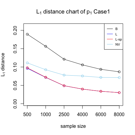
(a) $L_{1}$ error ($p_{1}$, Case 1)

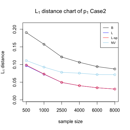
(b) $L_{1}$ error ($p_{1}$, Case 2)

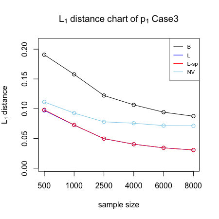
(c) $L_{1}$ error ($p_{1}$, Case 3)

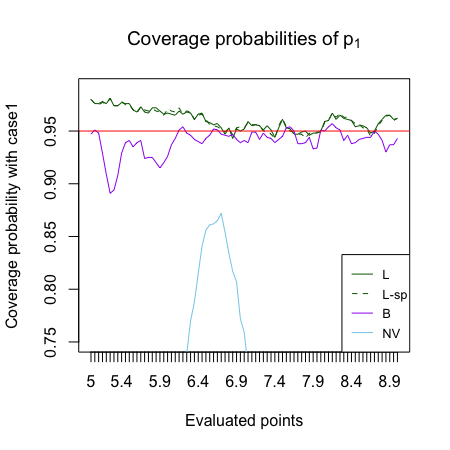
(d) CI coverage probability ($p_{1}$, Case 1, $n=8000$)

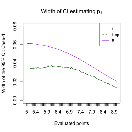
(e) Average CI width ($p_{1}$, Case 1, $n=8000$)

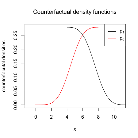
(f) True $p_{1}$ and $p_{0}$

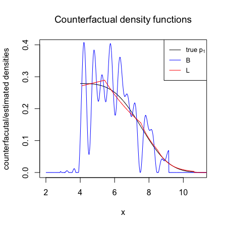
(g) Density estimates ($p_{1}$, Case 1, $n=4000$)

Figure 1: (a)–(c) Average $L_{1}$ distance between estimators and true $p_{1}$. In Cases 1, 2, and 3, both nuisance functions, only the propensity score, and only the conditional CDF are well-specified, respectively. (d) Empirical coverage probabilities of 95% CIs. (e) The corresponding widths for each CI from (d). The lines for L and L-sp cannot be visually distinguished for (a)–(e). (f) The true counterfactual density functions used for the simulations. “B”, “L”, “L-sp”, and “NV” stand for the basis expansion, log-concave, log-concave with sample splitting, and naive log-concave estimators, respectively. (g) The true density $p_{1}$ and the density estimates for $p_{1}$ by L and B from a single simulation based on $n=4000$ in Case 1.

Figures 1(a)–1(c) display the average $L_{1}$ distances of the estimators of $p_{1}$ as a function of $n$ in the three nuisance estimation scenarios. The results for $p_{0}$ are very similar, and can be found in the supplementary material. Our proposed log-concave estimator consistently had the smallest average $L_{1}$ distance of the three methods for all $n$ values. The average $L_{1}$ distance decreased as a function of $n$ for our estimator and the basis expansion estimator, but not for the naive log-concave estimator, which was expected because the counterfactual and marginal densities are different due to confounding. The average $L_{1}$ distances for our method with and without sample splitting were very similar. We expect the difference to be more substantial if more complicated nuisance estimators were used. The average $L_{1}$ distances were similar across the three nuisance estimator specifications, validating the double-robustness of the log-concave and basis expansion methods.

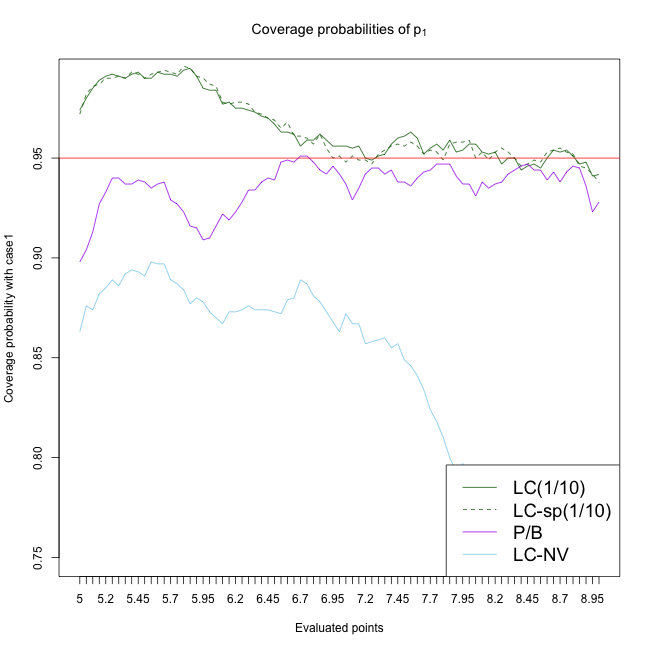
(a) $p_{1}$; C1; $n=500$

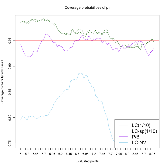
(b) $p_{1}$; C1; $n=1000$

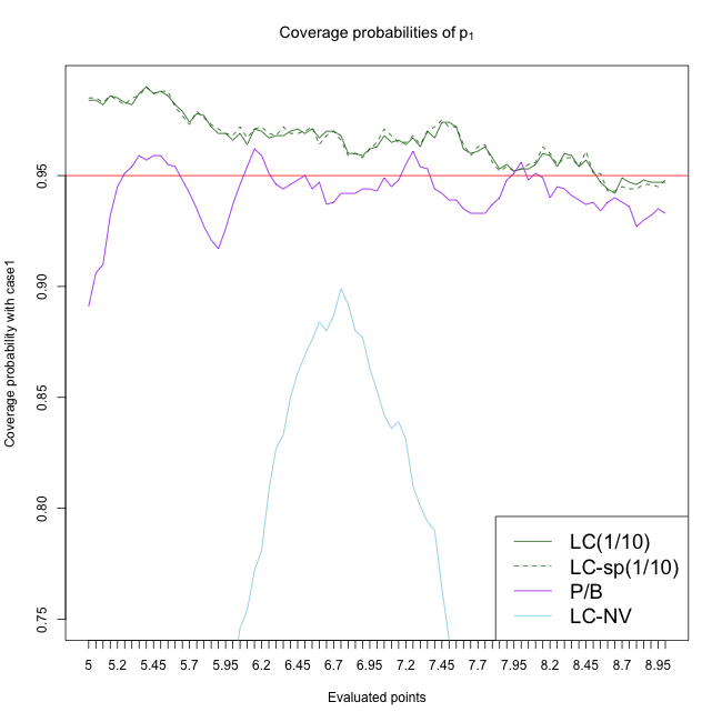
(c) $p_{1}$; C1; $n=2500$

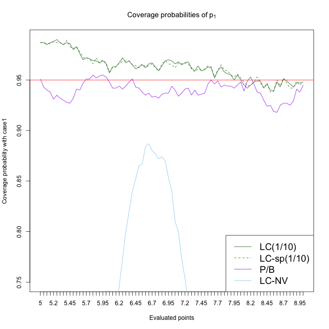
(d) $p_{1}$; C1; $n=4000$

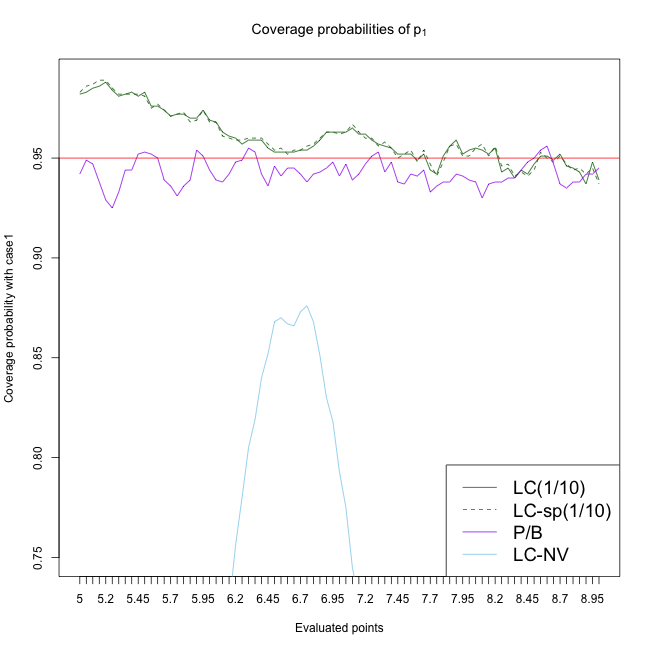
(e) $p_{1}$; C1; $n=6000$

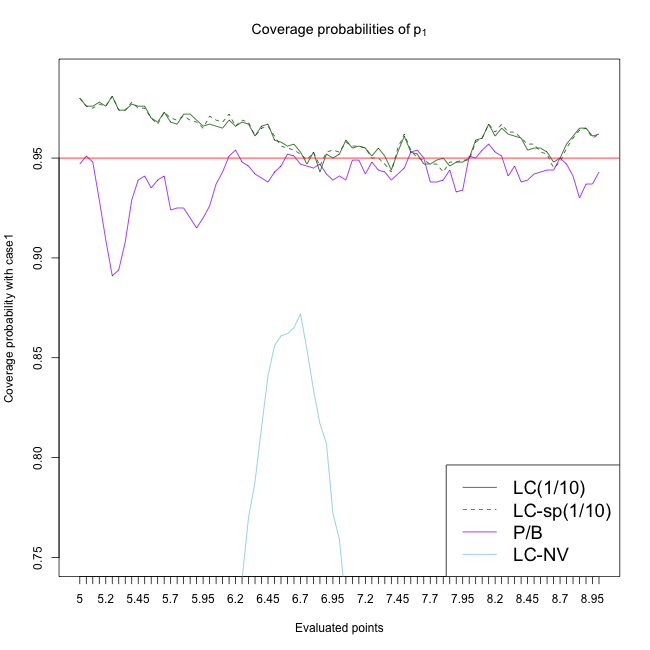
(f) $p_{1}$; C1; $n=8000$

Figure 10: The above displays are coverage probabilities of our proposed log-concave projection estimator’s 95% CIs with the suggested tuning parameter $b=1/10$ which is labeled as LC (see Section 5.2.1), and the coverage probabilities from 95% CI of projection basis method by Kennedy et al. (2023) which is denoted by P and B. For the projection basis method, the number of basis functions is the oracle number of functions which achieved the lowest average $L_{1}$ distance in each setting. “sp” stands for our sample splitting based estimator (see (30)). And, “NV” denotes the naive log-concave MLE. The coverage probabilities are measured in 81 equally spaced points in the domain. Each subcaption describes the estimand ($p_{1}$ or $p_{0}$), the sample size, and each case of nuisance estimations (Case 1, 2, or 3 abbreviated to C1, C2, and C3, respectively).

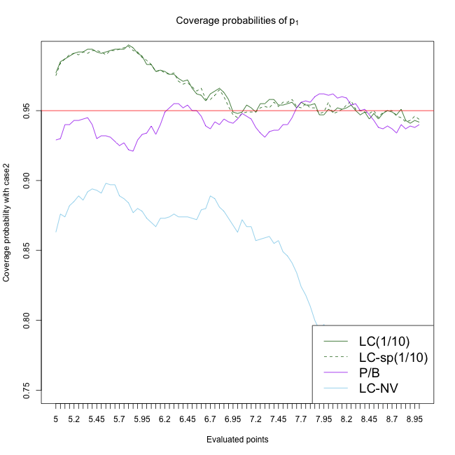
(a) $p_{1}$; C2; $n=500$

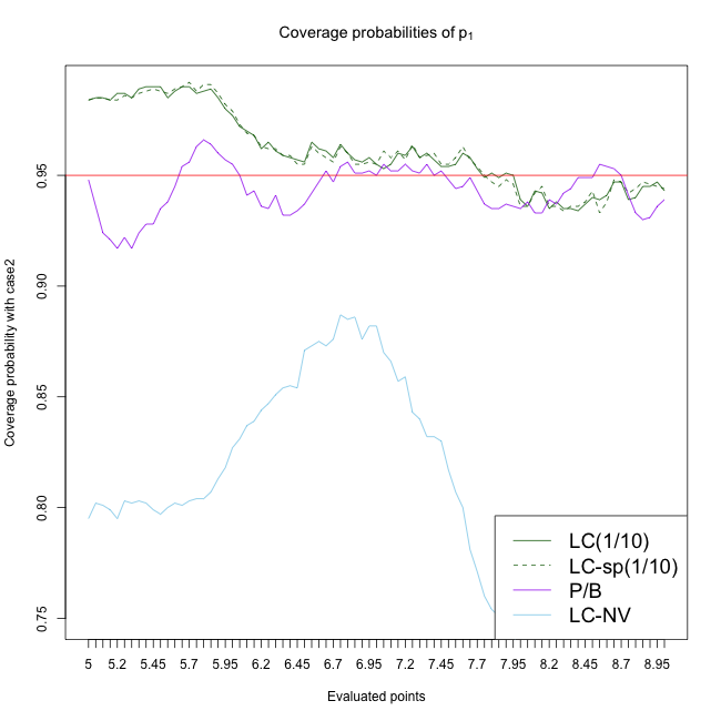
(b) $p_{1}$; C2; $n=1000$

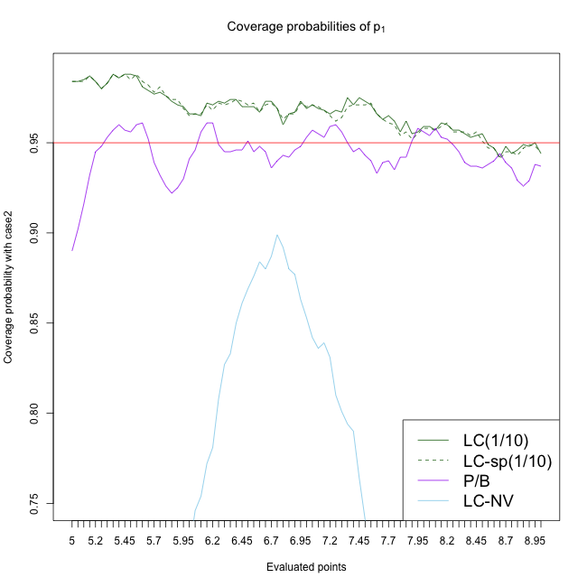
(c) $p_{1}$; C2; $n=2500$

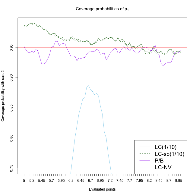
(d) $p_{1}$; C2; $n=4000$

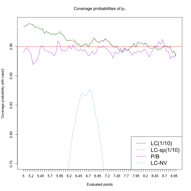
(e) $p_{1}$; C2; $n=6000$

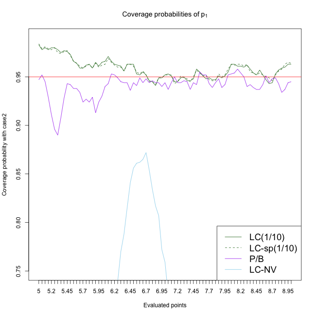
(f) $p_{1}$; C2; $n=8000$

Figure 11: Notational details can be found in Figure 10.

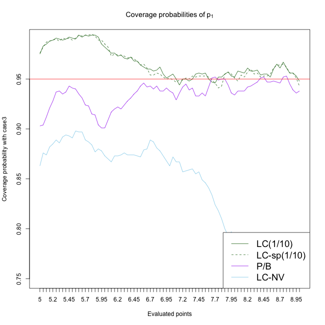
(a) $p_{1}$; C3; $n=500$

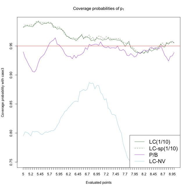
(b) $p_{1}$; C3; $n=1000$

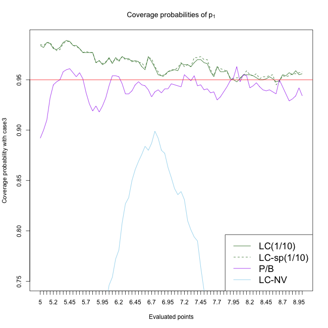
(c) $p_{1}$; C3; $n=2500$

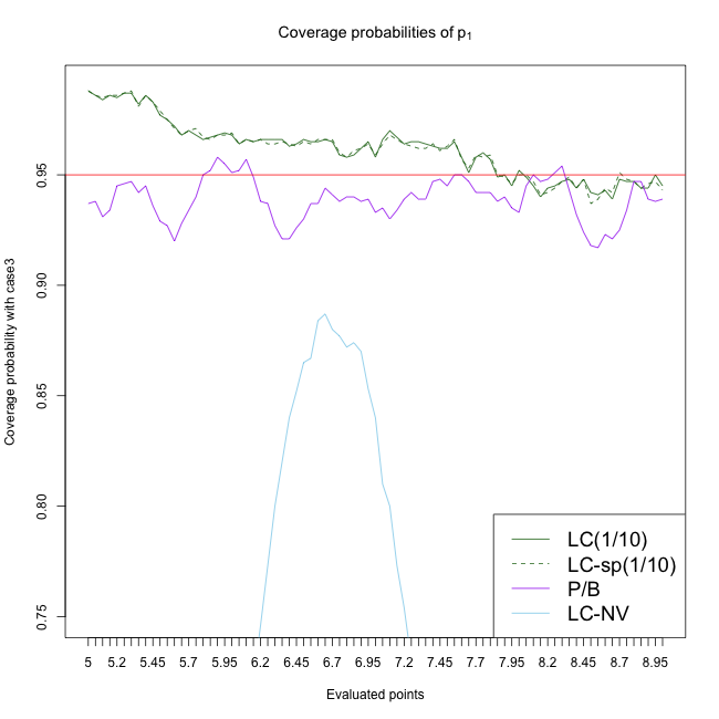
(d) $p_{1}$; C3; $n=4000$

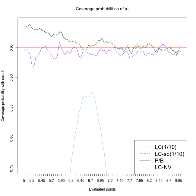
(e) $p_{1}$; C3; $n=6000$

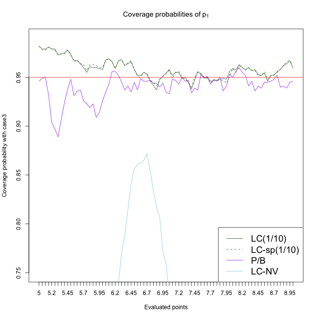
(f) $p_{1}$; C3; $n=8000$

Figure 12: Notational details can be found in Figure 10.

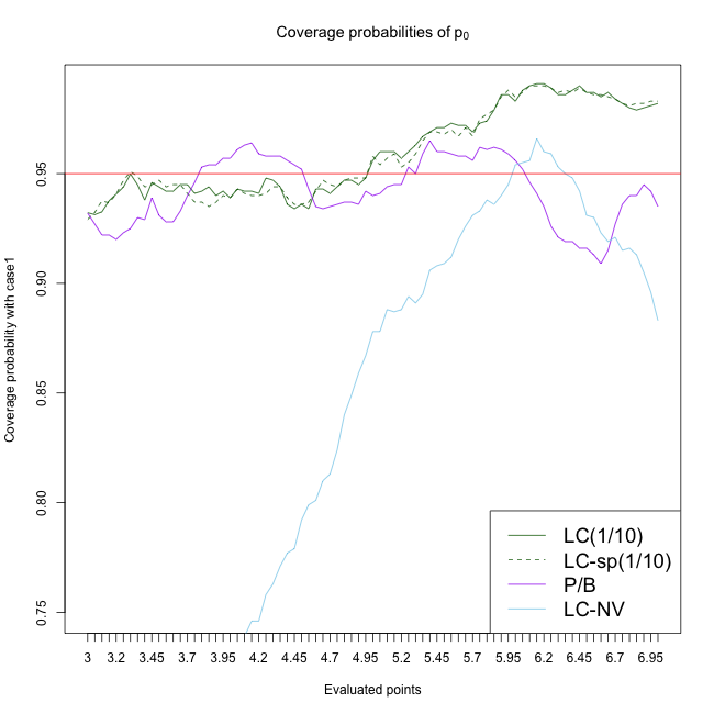
(a) $p_{0}$; C1; $n=500$

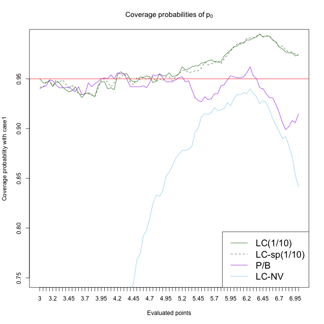
(b) $p_{0}$; C1; $n=1000$

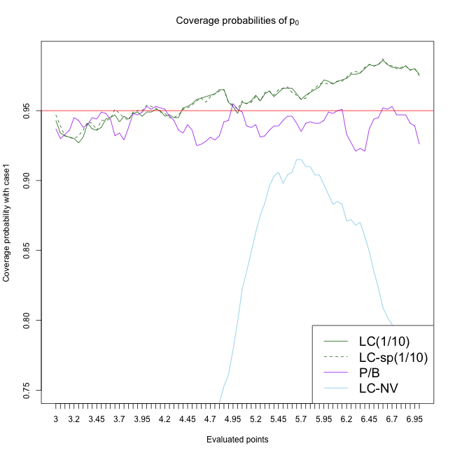
(c) $p_{0}$; C1; $n=2500$

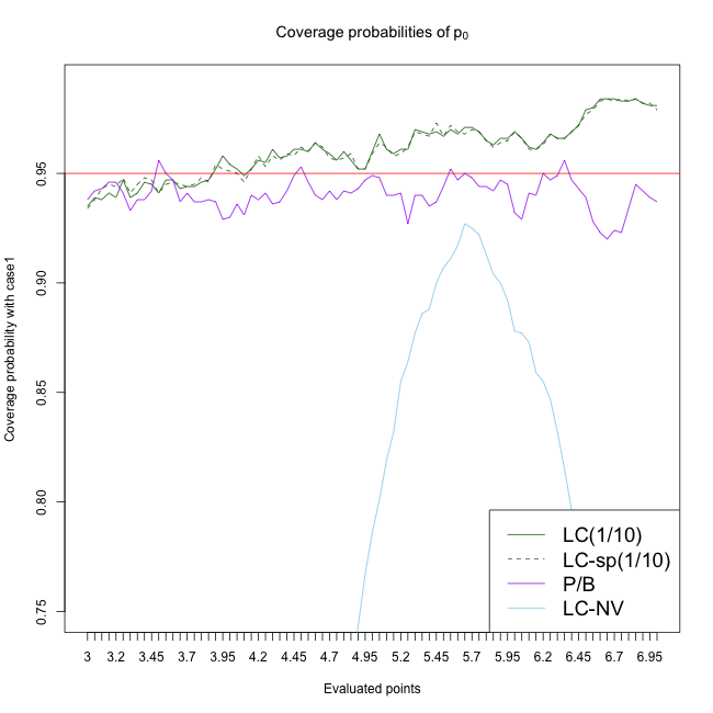
(d) $p_{0}$; C1; $n=4000$

(e) $p_{0}$; C1; $n=6000$

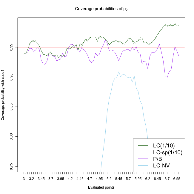
(f) $p_{0}$; C1; $n=8000$

Figure 13: Notational details can be found in Figure 10.

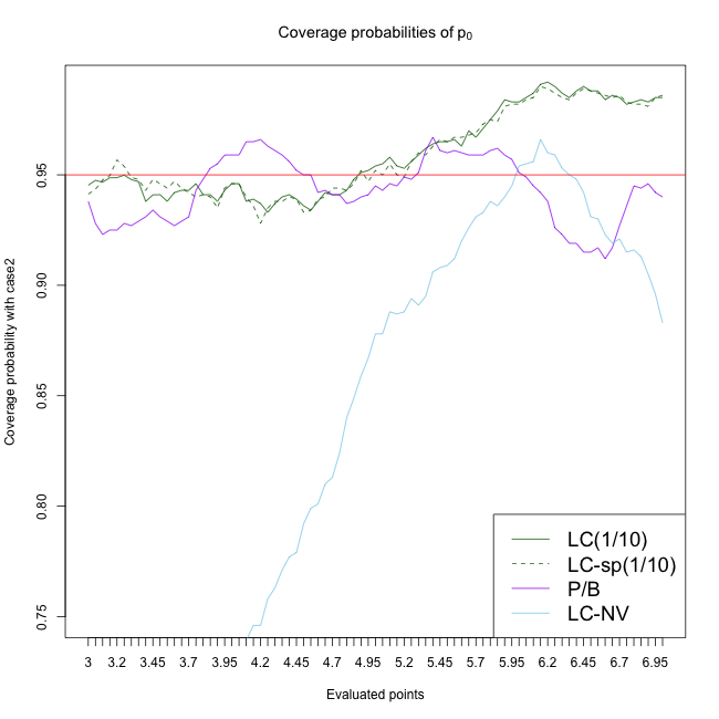
(a) $p_{0}$; C2; $n=500$

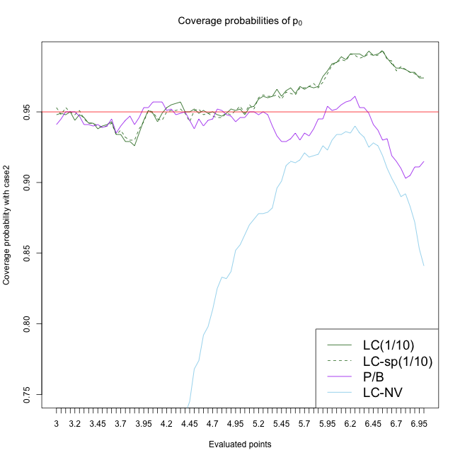
(b) $p_{0}$; C2; $n=1000$

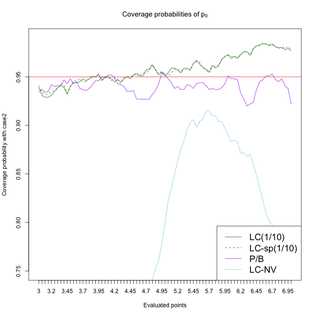
(c) $p_{0}$; C2; $n=2500$

(d) $p_{0}$; C2; $n=4000$

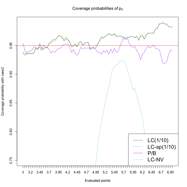
(e) $p_{0}$; C2; $n=6000$

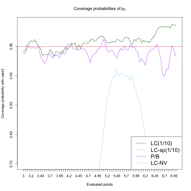
(f) $p_{0}$; C2; $n=8000$

Figure 14: Notational details can be found in Figure 10.

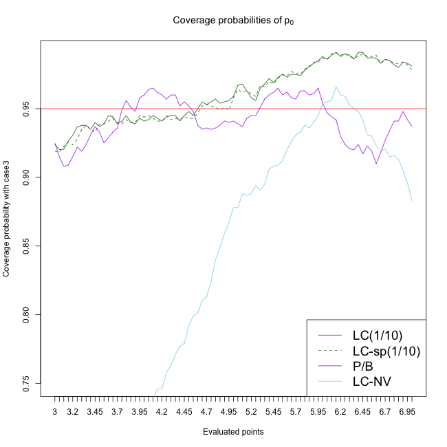
(a) $p_{0}$; C3; $n=500$

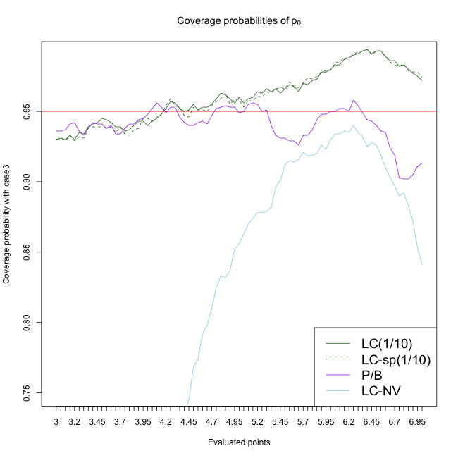
(b) $p_{0}$; C3; $n=1000$

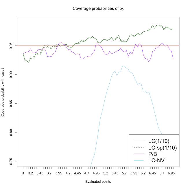
(c) $p_{0}$; C3; $n=2500$

(d) $p_{0}$; C3; $n=4000$

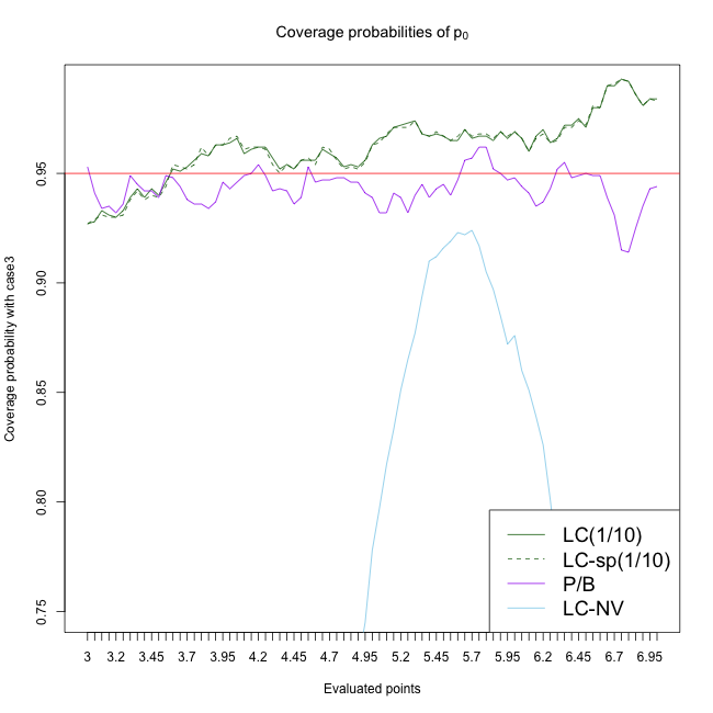
(e) $p_{0}$; C3; $n=6000$

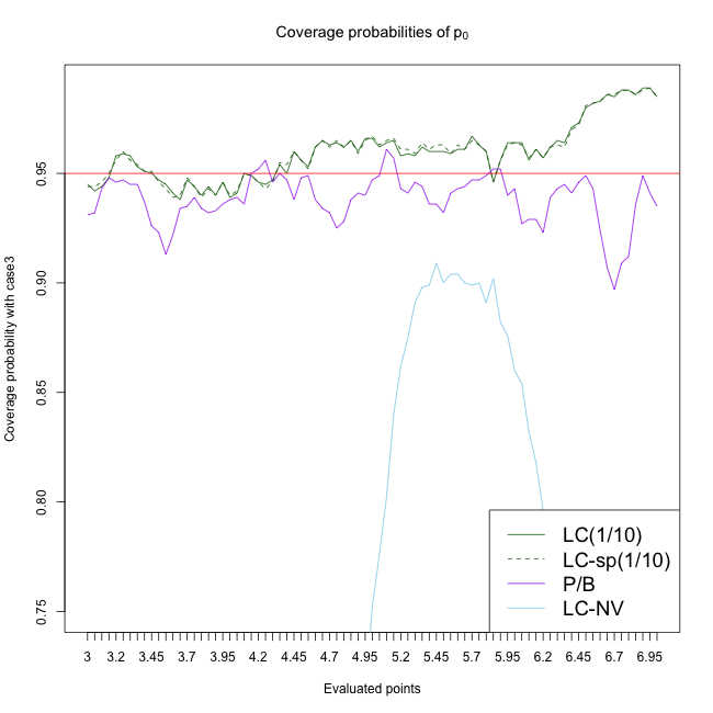
(f) $p_{0}$; C3; $n=8000$

Figure 15: Notational details can be found in Figure 10.

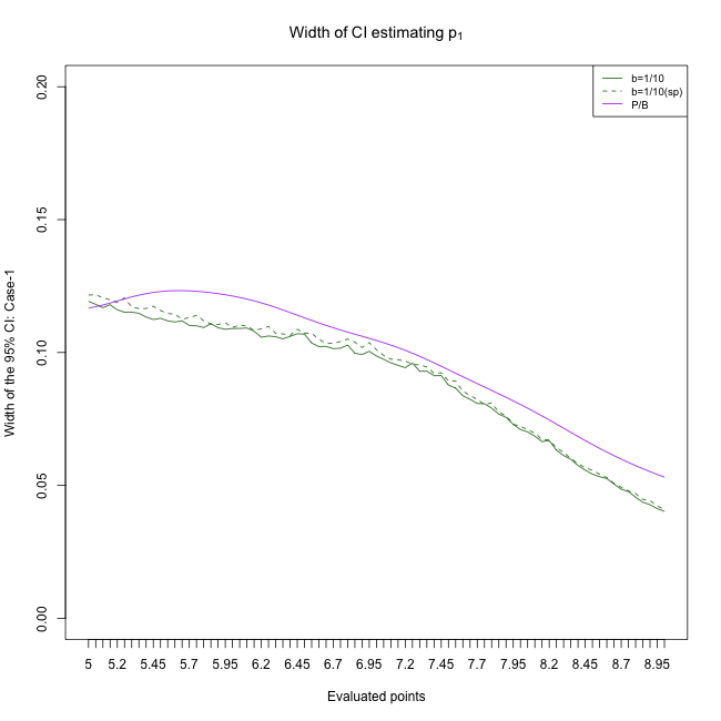
(a) $p_{1}$; C1; $n=500$

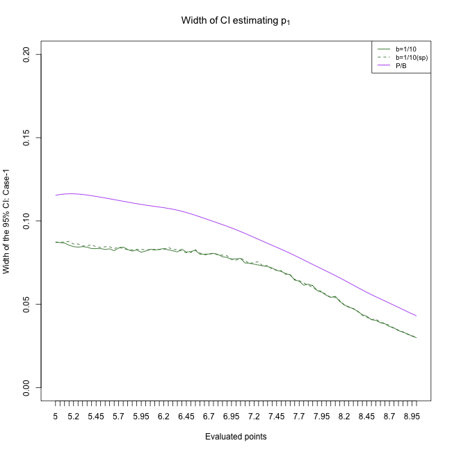
(b) $p_{1}$; C1; $n=1000$

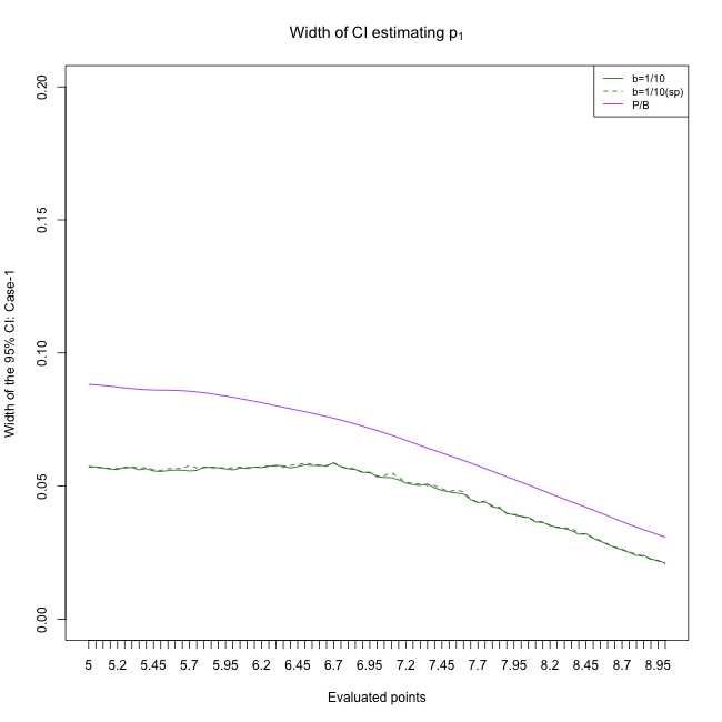
(c) $p_{1}$; C1; $n=2500$

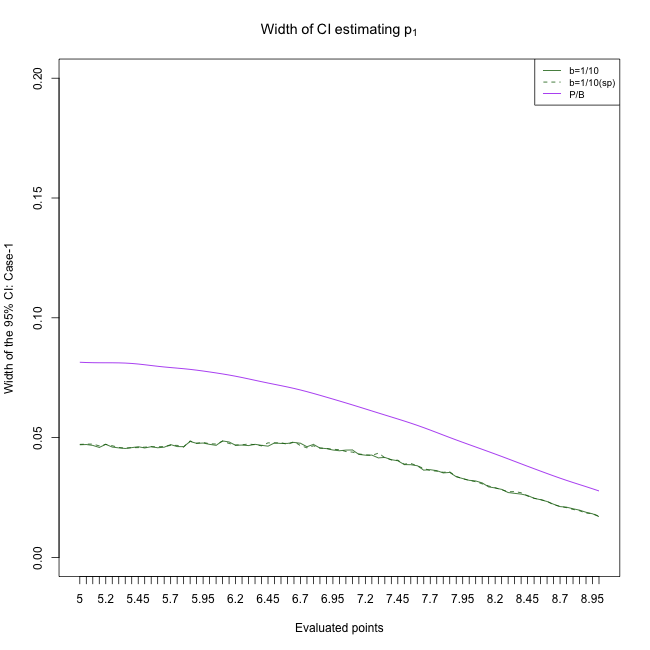
(d) $p_{1}$; C1; $n=4000$

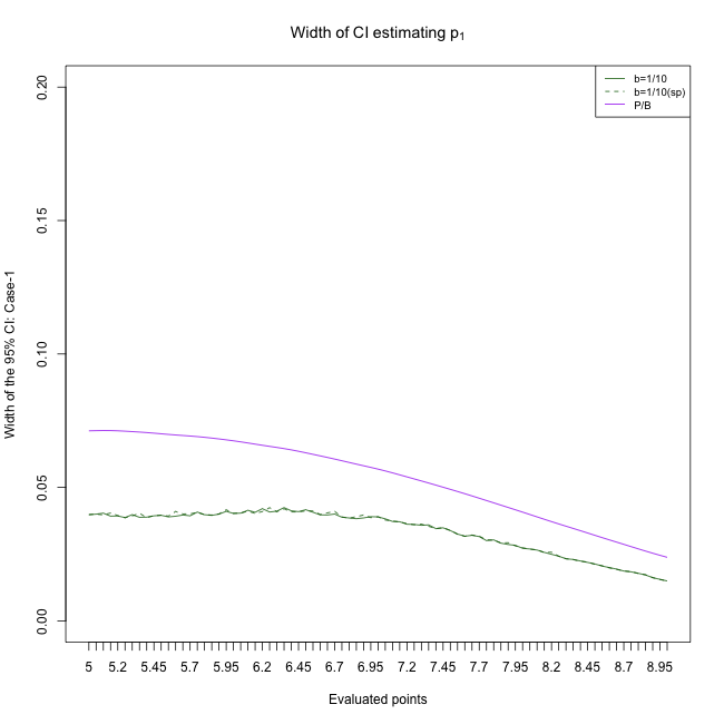
(e) $p_{1}$; C1; $n=6000$

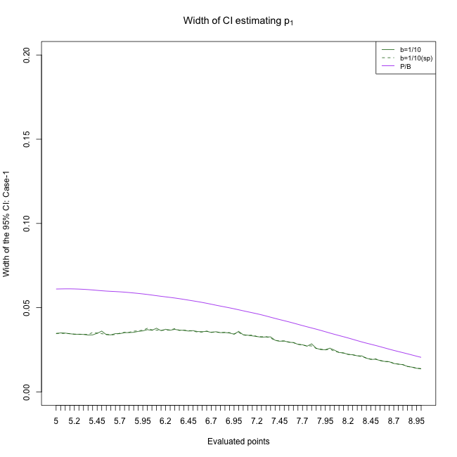
(f) $p_{1}$; C1; $n=8000$

Figure 16: The above displays are widths of our proposed log-concave projection estimator’s 95% CIs with the suggested tuning parameter $b=1/10$ which is labeled as LC (see Section 5.2.1), and the widths from 95% CI of projection basis method by Kennedy et al. (2023) which is denoted by P and B. For the projection basis method, the number of basis functions is the oracle number of functions which achieved the lowest average $L_{1}$ distance in each setting. “sp” stands for our sample splitting based estimator (see (30)). The widths are measured in 81 equally spaced points in the domain. Each subcaption describes the estimand ($p_{1}$ or $p_{0}$), the sample size, and each case of nuisance estimations (Case 1, 2, or 3 abbreviated to C1, C2, and C3, respectively). Since the difference between the cross-fitted procedure and the non-sample splitting procedure is insignificant, it is not visually distinguishable.

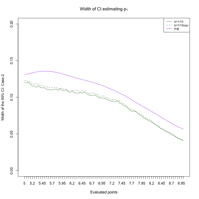
(a) $p_{1}$; C2; $n=500$

(b) $p_{1}$; C2; $n=1000$

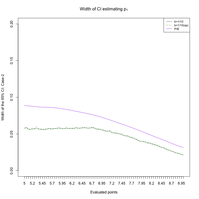
(c) $p_{1}$; C2; $n=2500$

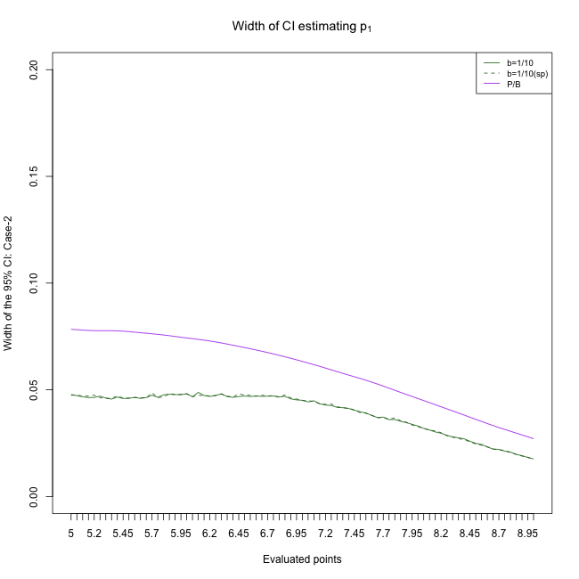
(d) $p_{1}$; C2; $n=4000$

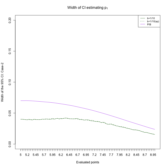
(e) $p_{1}$; C2; $n=6000$

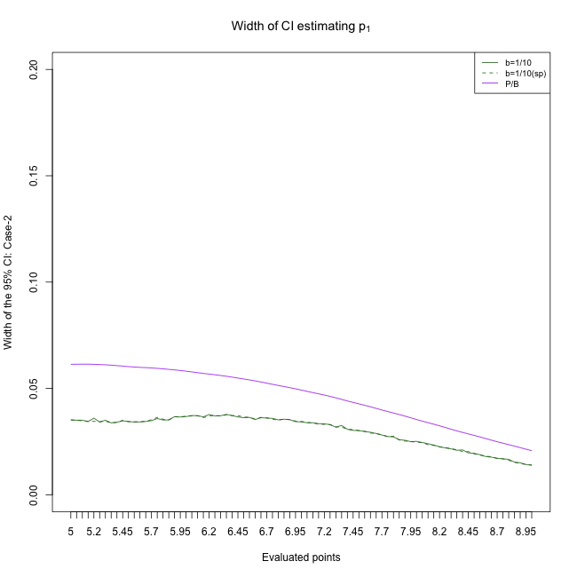
(f) $p_{1}$; C2; $n=8000$

Figure 17: Notational details can be found in Figure 16.

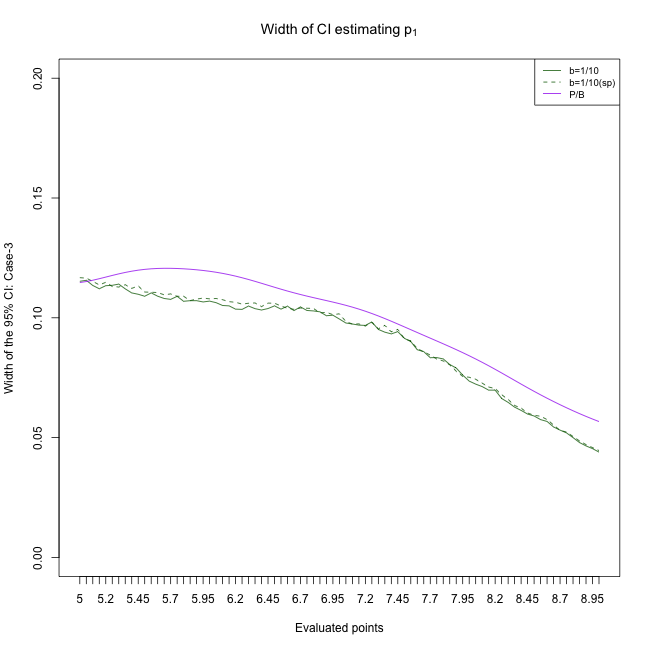
(a) $p_{1}$; C3; $n=500$

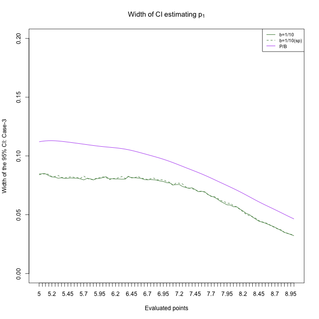
(b) $p_{1}$; C3; $n=1000$

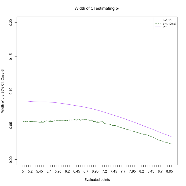
(c) $p_{1}$; C3; $n=2500$

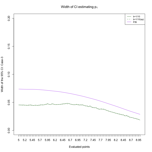
(d) $p_{1}$; C3; $n=4000$

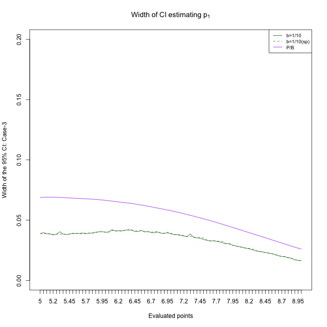
(e) $p_{1}$; C3; $n=6000$

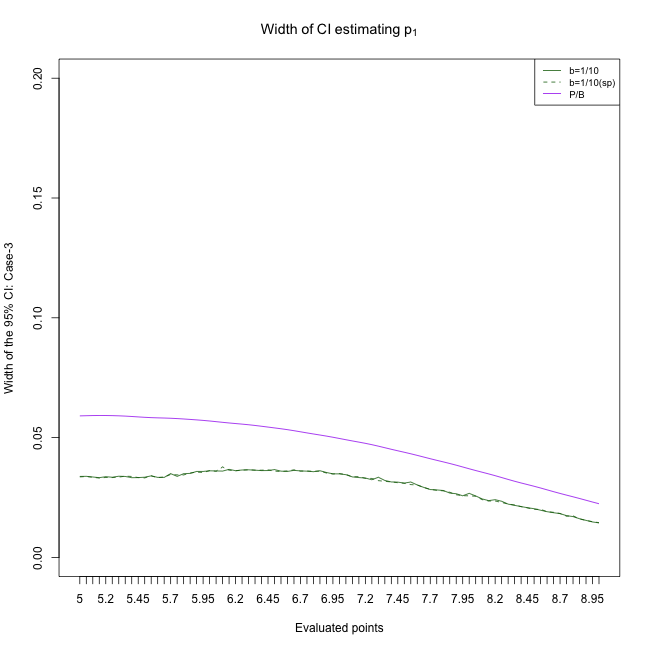
(f) $p_{1}$; C3; $n=8000$

Figure 18: Notational details can be found in Figure 16.

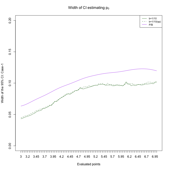
(a) $p_{0}$; C1; $n=500$

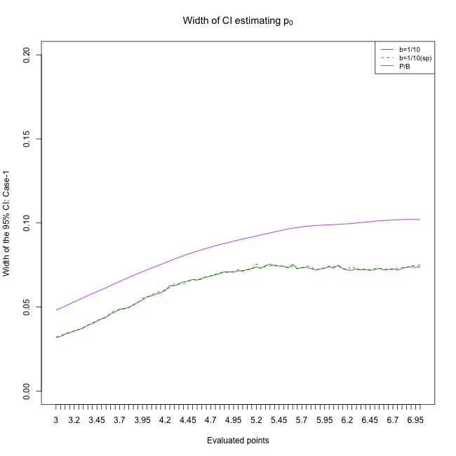
(b) $p_{0}$; C1; $n=1000$

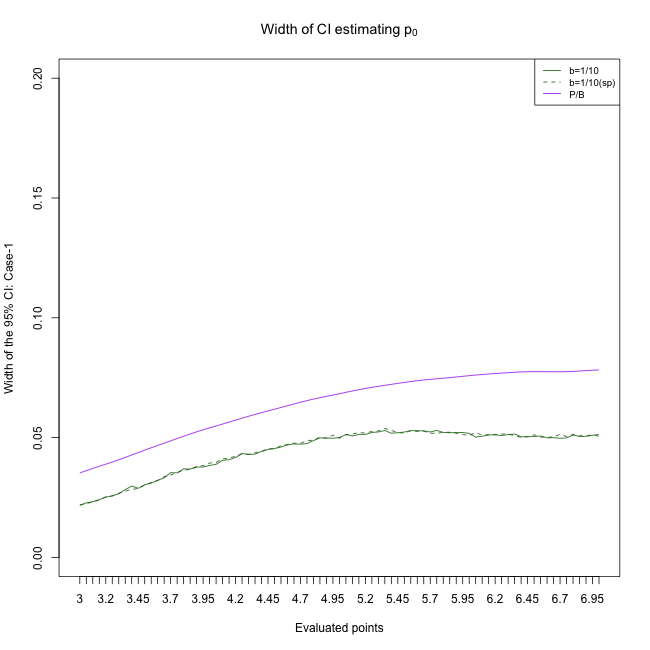
(c) $p_{0}$; C1; $n=2500$

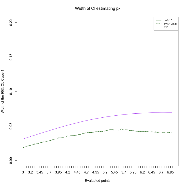
(d) $p_{0}$; C1; $n=4000$

(e) $p_{0}$; C1; $n=6000$

(f) $p_{0}$; C1; $n=8000$

Figure 19: Notational details can be found in Figure 16.

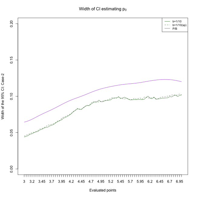
(a) $p_{0}$; C2; $n=500$

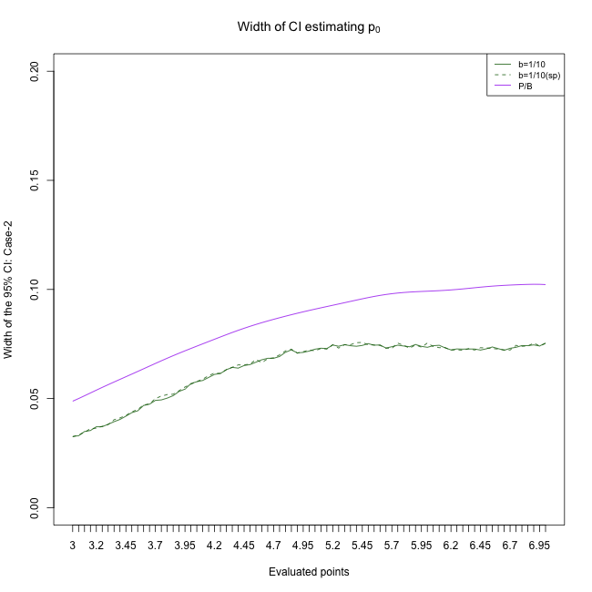
(b) $p_{0}$; C2; $n=1000$

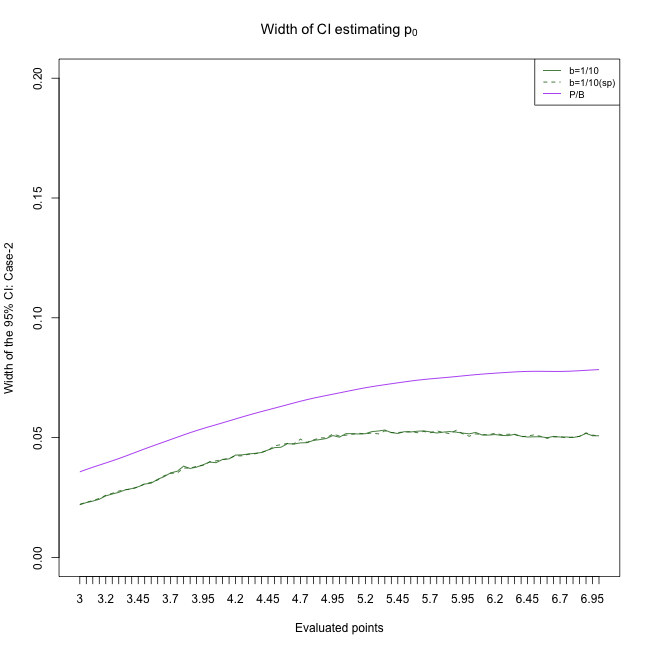
(c) $p_{0}$; C2; $n=2500$

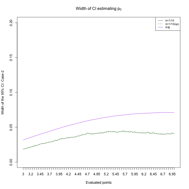
(d) $p_{0}$; C2; $n=4000$

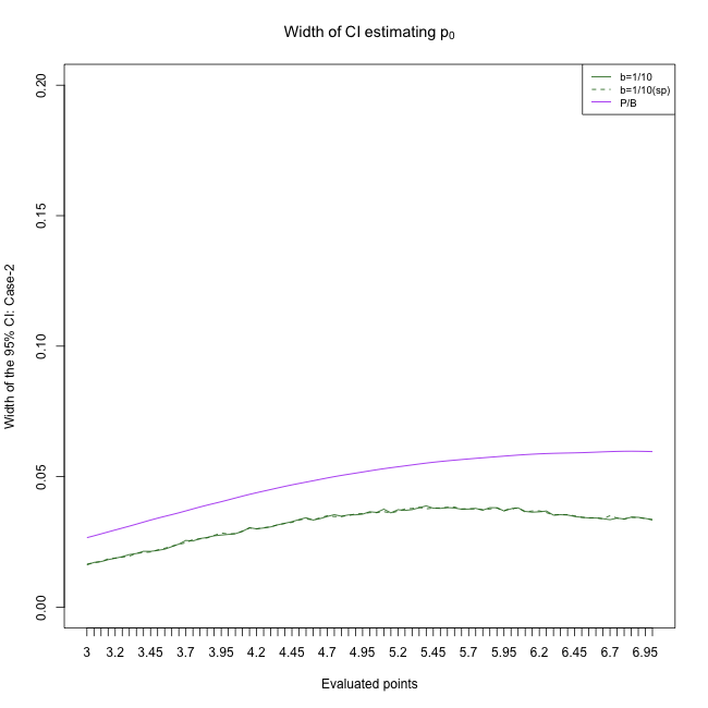
(e) $p_{0}$; C2; $n=6000$

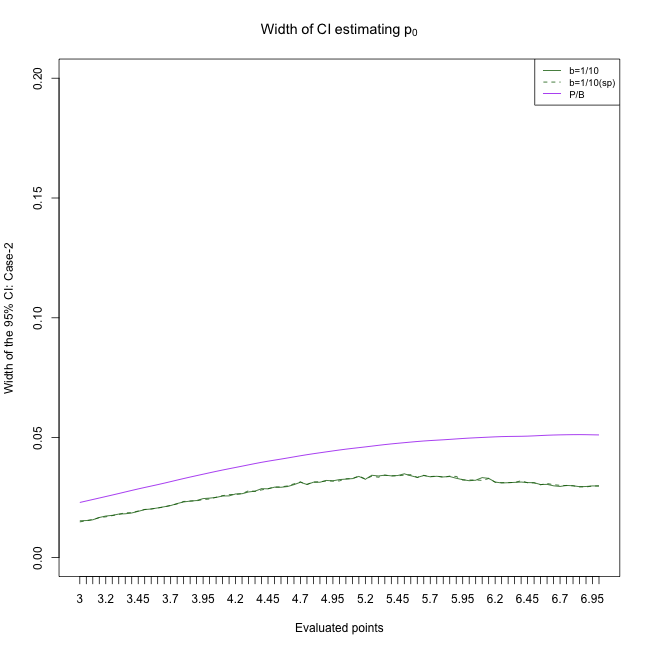
(f) $p_{0}$; C2; $n=8000$

Figure 20: Notational details can be found in Figure 16.

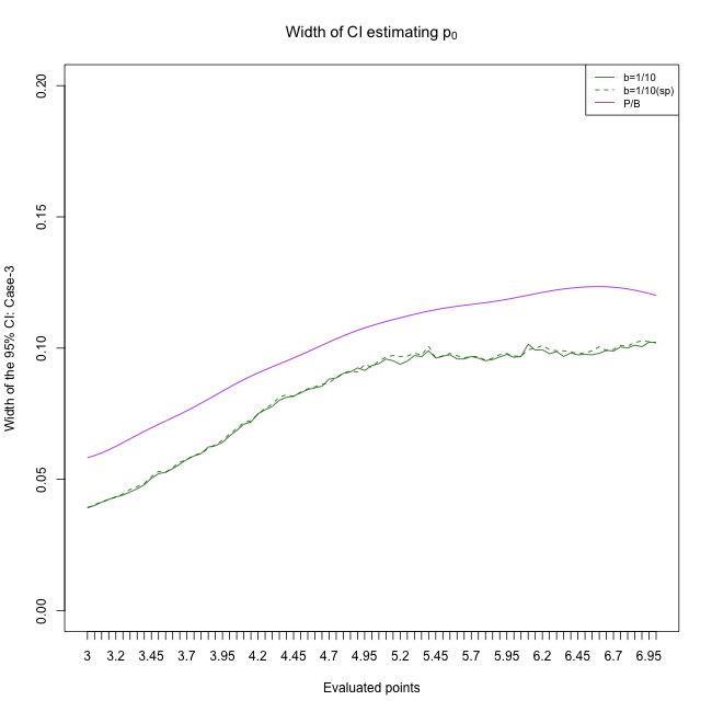
(a) $p_{0}$; C3; $n=500$

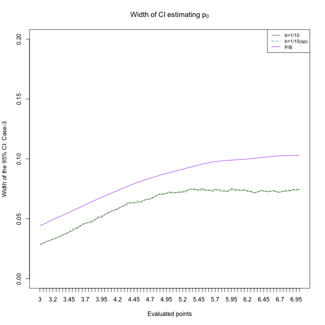
(b) $p_{0}$; C3; $n=1000$

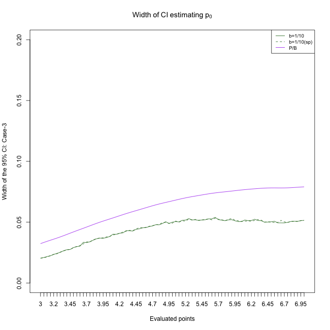
(c) $p_{0}$; C3; $n=2500$

(d) $p_{0}$; C3; $n=4000$

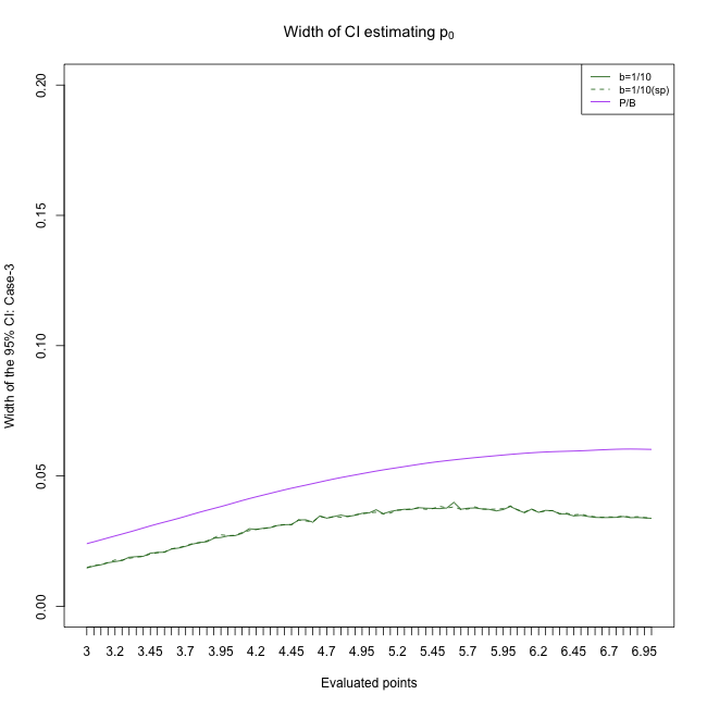
(e) $p_{0}$; C3; $n=6000$

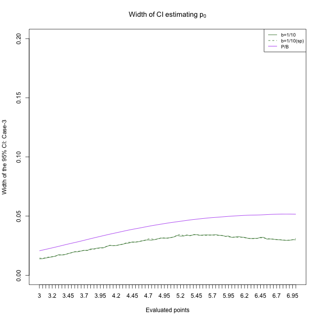
(f) $p_{0}$; C3; $n=8000$

Figure 21: Notational details can be found in Figure 16.

Figures 1(d)–1(e) display the coverage and average width of 95% CIs for $p_{1}$ for $n=8000$ in the well-specified nuisance scenario (Case 1). Figures 10–15 and 16–21 in the supplementary material display the results for other cases, $p_{0}$, and other sample sizes. Our CIs exhibited some undercoverage where the true density is close to zero when the sample size was smaller (i.e., $n=500,1000$), and exhibited overcoverage where the true density is large. Deng et al. (2022) observed similar phenomena in the non causal setting. Sample splitting did not meaningfully change coverage in this simulation design. The basis expansion method had substantial fluctuation in the coverage from point to point, including undercoverage for some points even with $n=8000$. This is because the basis expansion method is centered around an approximation to the density rather than around the true density, and this bias interferes with constructing CI’s with valid coverage. The average width of 95% CI’s for our method were also smaller than that of the basis expansion method in all sample sizes and cases. Figure 1(g) displays a single simulation result in Case 1 for estimating $p_{1}$ with $n=4000$. The number of basis function was 26, which was selected because it minimized average $L_{1}$ distance as described above. As opposed to our estimator, the basis expansion method suffers from boundary issues as well as instability across the domain, which might be exacerbated by the bounded support. Finally, the naive log-concave did not achieve nominal coverage in any case because it is inconsistent, demonstrating again that covariate adjustment in the causal setting is essential for valid estimation and inference.

8 Data analysis

We use our method to analyze the lalonde dataset from the R package cobalt (Greifer, 2023). The data was used by Dehejia and Wahba (1999) to study the effectiveness of a job training program on earnings (LaLonde, 1986). The treatment $A$ is an indicator of participation in the National Supported Work Demonstration job training program. The data contains 185 people with $A=1$ and a comparison sample of 429 people with $A=0$ from the Population Survey of Income Dynamics. The outcome $Y$ is the real earnings in US dollars measured in 1978, several years after completion of the program. We scaled the outcome by $10^{4}$. The covariates include demographic variables (age, race, education, and marital status), and two previous earnings levels measured in 1974 and 1975, which we also scaled by $10^{4}$.

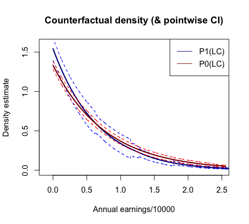
(a) 95% CIs

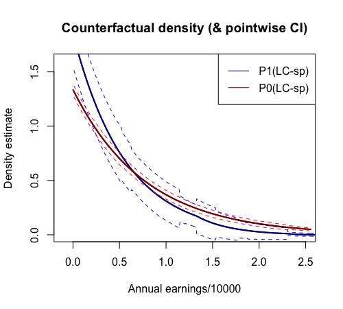
(b) 95% CI’s via sample splitting

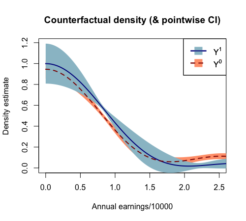
(c) 95% CI’s via projection method

Figure 2: Density estimates and corresponding 95% pointwise CIs for the Lalonde data. P1 and P0 stand for the counterfactual density estimates for each treatment and control group, respectively. (a) Our log-concave estimator. (b) Our estimator with five-fold sample splitting. (c) Basis expansion estimator (Kennedy et al., 2023).

We estimated the density of real earnings in 1978 for treatment and control using our proposed method adjusting for the covariates listed above. We estimated the conditional distribution function using the location-scale estimator with a gamma distribution as in Lemma 1. We estimated the propensity score and the conditional mean of the outcome using random forests via the R package ranger (Wright and Ziegler, 2017). For the conditional mean, we included interactions between the treatment and covariates as additional predictors in the random forest. To estimate the conditional variance, we used another random forest with these same predictors and outcome $(Y_{i}-\hat{\mu}_{i})^{2}$, where $\hat{\mu}_{i}$ is the fitted value of the conditional mean for the $i$th observation. We considered other several other conditional distribution estimators, including location-scale estimators with exponential and uniform CDFs, as well as quantile regression random forest (Meinshausen and Ridgeway, 2006; Elie-Dit-Cosaque and Maume-Deschamps, 2022). We did not find significant differences between the results, so we only present the results from the gamma conditional distribution function. We also computed the log-concave estimator with sample splitting with $K_{0}=5$ folds and the same nuisance estimators as above (see Section 6). We set the tuning parameter for estimating $\chi_{\theta_{a}}$ to be $n^{-1/10}$. For comparison, we estimated the counterfactual density and corresponding 95% CIs using the basis expansion method (Kennedy et al., 2023) using the cdensity function in the R package npcausal (Kennedy, 2023). We again used 5 fold sample splitting and random forests for the nuisance estimators.

Figure 2 displays the estimated densities. The densities under treatment and control are similar in shape, but perhaps surprisingly there are regions where the CI’s in the upper and lower tails do not overlap. This is particularly apparent in the results for the sample splitting estimator. This suggests that, if we believe we have accounted for all sources of confounding and that the true densities are log-concave, we have evidence of an effect of treatment on the distribution of income. By contrast, a 95% CI for the ATE (using the ate function in the npcausal package with default settings) was $[-0.10,0.56]$, indicating there was not a statistically significant difference in the counterfactual means. Our proposed log-concave estimator does not have the same boundary issue that the kernel density estimator and/or the projection method encounter on this dataset.

Appendix A Empirical processes tools

Given classes $\mathcal{F}_{1},\dots,\mathcal{F}_{k}$ of functions $\mathcal{F}_{i}:\mathcal{X}\mapsto\mathcal{R}$ and a function $\varphi:\mathbb{R}^{k}\mapsto\mathbb{R}$, let $\varphi(\mathcal{F}_{1},\dots,\mathcal{F}_{k})$ be the class of functions $x\mapsto\varphi(f_{1}(x),\dots,f_{k}(x))$, where $f_{i}\in\mathcal{F}_{i}$, for $i=1,\dots,k$. The following proposition is Theorem 3 in van der Vaart and Wellner (2000).

Proposition 1.

Suppose that $\mathcal{F}_{1},\dots,\mathcal{F}_{k}$ are $P$-Glivenko-Cantelli classes of functions, and that $\varphi:\mathbb{R}^{k}\mapsto\mathbb{R}$ is continuous. Then $\mathcal{H}:=\varphi(\mathcal{F}_{1},\dots,\mathcal{F}_{k})$ is a $P$-Glivenko-Cantelli class given that it has an integrable envelope.

The following lemma that controls empirical process terms under sample splitting scheme and its proof were provided in Lemma C.3 of Kim et al. (2018).

Lemma 6.

(Sample-splitting). Let ${\mathbb{P}}_{n}$ denote the empirical measure over a set $D_{1,n}=(Z_{1},\cdots,Z_{n})$, which is i.i.d. from ${\mathbb{P}}$. Let $\hat{f}$ be a sample operator (e.g., estimator) constructed in a separate, independent sample set $D_{2,m}$ with m observations. Then we have

$${\mathbb{P}}\Big{(}({\mathbb{P}}_{n}-{\mathbb{P}})\hat{f}\Big{)}^{2}\leq\frac{1}{n}{\mathbb{P}}\hat{f}^{2}$$

We state the following proposition that controls empirical processes indexed by classes of functions that change with $n$. It is Theorem 2.11.22 in van der Vaart and Wellner (1996). For each $n$, suppose that a class of measurable functions $\mathcal{F}_{n}=\{f_{n,t}:t\in T\}$ indexed by a totally bounded semimetric space $(T,\rho)$ admits an envelope function (sequence) $F_{n}$. And, further suppose that the classes $\mathcal{F}_{n,\delta}=\{f_{n,s}-f_{n,t}:\rho(s,t)<\delta\}$ and $\mathcal{F}^{2}_{n,\delta}$ are measurable under the probability measure $P$.

Proposition 2.

Suppose that the following holds,

$$\begin{split}&PF_{n}^{2}=O(1),\\ &PF_{n}^{2}I(F_{n}>\eta\sqrt{n})\rightarrow 0,\qquad{\rm for~{}every~{}}\eta>0,\\ \sup_{\rho(s,t)<\delta_{n}}&P(f_{n,s}-f_{n,t})^{2}\rightarrow 0,\qquad{\rm for~{}every~{}}\delta_{n}\downarrow 0,\\ \end{split}$$ (37)

and,

$$\sup_{Q}\int_{0}^{\delta_{n}}\sqrt{\log N\left(\epsilon\|F_{n}\|_{Q,2},\mathcal{F}_{n},L_{2}(Q)\right)}d\epsilon\rightarrow 0,\qquad{\rm for~{}every~{}}\delta_{n}\downarrow 0.$$ (38)

Then the sequence $\{\sqrt{n}({\mathbb{P}}_{n}-P)f_{n,t}:t\in T\}$ is asymptotically tight in $\ell^{\infty}(T)$. Moreover, given that the sequence of covariance functions $Pf_{n,s}f_{n,t}-Pf_{n,s}Pf_{n,t}$ converges pointwise on $T\times T$, the sequence $\{\sqrt{n}({\mathbb{P}}_{n}-P)f_{n,t}:t\in T\}$ converges in distribution to a Gaussian process.

Here we state the following proposition that gives bounds for each $L_{p}$-norm of ${\mathbb{G}}_{n}=\sqrt{n}({\mathbb{P}}_{n}-P)$ for function classes $\mathcal{F}$ that admit a finite uniform entropy integral.

Proposition 3.

Let $\mathcal{F}$ be a $P$-measurable class of measurable functions with measurable envelope function $F$. Then,

$$\left\|\|{\mathbb{G}}_{n}\|_{\mathcal{F}}\right\|_{P,p}\lesssim J(1,\mathcal{F})\|F\|_{P,2\vee p},\qquad 1\leq p,$$

where the entropy integral $J(1,\mathcal{F})$ is given by

$$J(1,\mathcal{F})=\sup_{Q}\int_{0}^{\delta}\sqrt{1+\log N\left(\epsilon\|F\|_{Q,2},\mathcal{F},L_{2}(Q)\right)}d\epsilon,$$

where the supremum is taken over all discrete probability measures $Q$ with $\|F\|_{Q,2}>0$.

Appendix B Proofs of theorems, lemmas

B.1 Proof of Lemma 1

First, we show (E1), since (E3) is trivial. Under the conditions in Lemma 1, we have

$$P_{*}\int_{\mathbb{R}}\left|H\left(\frac{s-\hat{\mu}_{a}(\mathbf{X})}{\hat{\sigma}_{a}(\mathbf{X})}\right)-H\left(\frac{s-\mu_{a,\infty}(\mathbf{X})}{\sigma_{a,\infty}(\mathbf{X})}\right)\right|ds$$

$$\indent\leq P_{*}\int_{\mathbb{R}}L(s)\left|\frac{s-\hat{\mu}_{a}(\mathbf{X})}{\hat{\sigma}_{a}(\mathbf{X})}-\frac{s-\mu_{a,\infty}(\mathbf{X})}{\sigma_{a,\infty}(\mathbf{X})}\right|ds$$

$$\indent\leq P_{*}\int_{\mathbb{R}}L(s)\left|\frac{s(\hat{\sigma}_{a}(\mathbf{X})-\sigma_{a,\infty}(\mathbf{X}))}{\hat{\sigma}_{a}(\mathbf{X})\sigma_{a,\infty}(\mathbf{X})}+\frac{\hat{\sigma}_{a}(\mathbf{X})(\mu_{a,\infty}(\mathbf{X})-\hat{\mu}_{a}(\mathbf{X}))+\hat{\mu}_{a}(\mathbf{X})(\hat{\sigma}_{a}(\mathbf{X})-\sigma_{a,\infty}(\mathbf{X}))}{\hat{\sigma}_{a}(\mathbf{X})\sigma_{a,\infty}(\mathbf{X})}\right|ds$$

$$\indent\leq P_{*}\int_{\mathbb{R}}L(s)\left[(K^{2}|s|+K^{3})|\hat{\sigma}_{a}(\mathbf{X})-\sigma_{a,\infty}(\mathbf{X})|+K|\hat{\mu}_{a}(\mathbf{X})-\mu_{a,\infty}(\mathbf{X})|\right]ds\rightarrow 0.$$

Now, we show (EC1) and (EC2). For each $\epsilon>0$, there exists $0<\epsilon_{0}<1$ which satisfies $H(s)<\epsilon$ when $s\leq K(H^{-1}(\epsilon_{0})+K)$, and $1-H(s)<\epsilon$ when $s\geq K(H^{-1}(1-\epsilon_{0})-K)$. Define $L:=\max_{s\in\mathbb{R}}L(s)$ and $L_{\epsilon_{0}}$ as a Lipschitz constant for $H^{-1}$ on the interval $[\epsilon_{0},1-\epsilon_{0}]$. We further let $K_{H,\epsilon_{0}}$ as $\max\{|H^{-1}(\epsilon_{0})|,|H^{-1}(1-\epsilon_{0})|\}$. By the bracketing number condition on the class $\mathcal{F}_{1}\times\mathcal{F}_{2}$, we have finite number of brackets $(f_{l,i},g_{l,i}),\,(f_{u,i},g_{u,i})$ where $L_{1}((f_{l,i},g_{l,i}),(f_{u,i},g_{u,i}))(P_{*})\leq\epsilon/(2L(K^{3}+K_{H,\epsilon_{0}}))$ for $1\leq i\leq N_{\epsilon}$ where $N_{\epsilon}=N_{\epsilon,L,K,K_{H,\epsilon_{0}}}=N_{[]}(\epsilon/(2L(K^{3}+K_{H,\epsilon_{0}})),\mathcal{F}_{1}\times\mathcal{F}_{2},L_{1}(P_{*}))$. Now we construct the brackets for the class $\mathcal{F}_{H}$ at $H((s-f)/g)$ by $H((H^{-1}(\epsilon_{j})-f_{u,i})/g_{u,i})$, $H((H^{-1}(\epsilon_{j+i})-f_{l,i})/g_{l,i})$, where $(f,g)$ has lower and upper brackets $(f_{l,i},g_{l,i}),(f_{u,i},g_{u,i})$ and $H^{-1}(\epsilon_{j})\leq s<H^{-1}(\epsilon_{j+1})$, and $0\leq(\epsilon_{j+1}-\epsilon_{j})\leq\epsilon/(2LL_{\epsilon_{0}}K)$ for $1\leq i\leq N^{\prime}_{\epsilon}-1$, $\epsilon_{1}=\epsilon_{0},\,\epsilon_{N^{\prime}_{\epsilon}}=1-\epsilon_{0}$. As in Section B.1, assuming that $K>1$ without loss of generality, for $\epsilon_{0}\leq s\leq 1-\epsilon_{0}$, we have

$$P_{*}\left|H\left(\frac{H^{-1}(\epsilon_{j})-f_{u,i}}{g_{u,i}}\right)-H\left(\frac{H^{-1}(\epsilon_{j+1})-f_{l,i}}{g_{i,i}}\right)\right|$$

$$\indent\leq L\left[P_{*}\left|\frac{g_{u,i}(f_{u,i}-f_{l,i})+f_{u,i}(g_{u,i}-g_{l,i})}{g_{u,i}g_{i,i}}\right|\right.$$

$$\qquad\qquad\left.+P_{*}\left|\frac{g_{l,i}(H^{-1}(\epsilon_{j})-H^{-1}(\epsilon_{j+1}))+H^{-1}(\epsilon_{j+1})(g_{l,i}-g_{u,i})}{g_{u,i}g_{i,i}}\right|\right]$$

$$\indent\leq L(K^{3}+K_{H,\epsilon_{0}})L_{1}((f_{l,i},g_{l,i}),(f_{u,i},g_{u,i}))(P_{*})+LL_{\epsilon_{0}}K(\epsilon_{j+i}-\epsilon_{j})$$

$$\indent\leq\epsilon.$$

In addition, since $H(s)<\epsilon$ on $s\in(-\infty,K(H^{-1}(\epsilon_{0})+K)]$, $0$ and $H(K(H^{-1}(\epsilon_{0})+K)$ can serve as lower and upper bracket for any $H((s-f)/g)\in\mathcal{F}_{H}$ with $s\in(-\infty,K(H^{-1}(\epsilon_{0})+K)]$. Analogous brackets $1$ and $H(K(H^{-1}(1-\epsilon_{0})-K)$ work for the case $s\geq K(H^{-1}(1-\epsilon_{0})-K)$. Thus, we have $N_{[]}(\epsilon,\mathcal{F}_{H},L_{1}(P_{*}))\leq N_{\epsilon}N^{\prime}_{\epsilon}+2<\infty$, and this implies the condition (EC1).

To show (EC2), first we notice that, the primitive $\int_{-\infty}^{t}H((s-f)/g)ds$ is $gJ_{1}((t-f)/g)$ in $t\in(-\infty,0]$, similarly one can see the primitive $\int_{0}^{\infty}\left(1-H((s-f)/g)\right)ds$ is $gJ_{2}((t-f)/g)$ in $t\in[0,\infty)$. $J_{1}$ and $J_{2}$ are uniformly bounded on $(-\infty,0],\,[0,\infty)$ by sufficiently large $K_{J}>0$, respectively, since $H$ has finite first moment, which implies $\int_{-\infty}^{0}H(s)ds+\int_{0}^{\infty}\left(1-H(s)\right)ds<\infty$. Recalling that $\mathcal{F}_{2}$ is uniformly bounded by $K$, as in the derivation steps to show (EC1), there exists $M_{J_{1}}<0$ such that $J(s)<\epsilon$ when $s<K(J_{1}^{-1}(M_{J_{1}})+K)$, for each $\epsilon>0$. Now, for general bracket pairs, we have,

$$P_{*}\left|g_{l,i}J_{1}\left(\frac{J_{1}^{-1}(\epsilon_{j})-f_{u,i}}{g_{u,i}}\right)-g_{u,i}J_{1}\left(\frac{J_{1}^{-1}(\epsilon_{j+1})-f_{l,i}}{g_{i,i}}\right)\right|$$

$$\leq P_{*}\left|\left(g_{l,i}-g_{u,i}\right)J_{1}\left(\frac{J_{1}^{-1}(\epsilon_{j})-f_{u,i}}{g_{u,i}}\right)\right|$$

$$\indent\qquad+P_{*}\left|g_{u,i}\left[J_{1}\left(\frac{J_{1}^{-1}(\epsilon_{j})-f_{u,i}}{g_{u,i}}\right)-J_{1}\left(\frac{J_{1}^{-1}(\epsilon_{j+1})-f_{l,i}}{g_{i,i}}\right)\right]\right|$$

$$\indent\leq K_{J}P_{*}\left|g_{u,i}-g_{l,i}\right|+L_{J_{1}}KP_{*}\left|\frac{g_{u,i}(f_{u,i}-f_{l,i})+f_{u,i}(g_{u,i}-g_{l,i})}{g_{u,i}g_{i,i}}\right|$$

$$\qquad\qquad+L_{J_{1}}KP_{*}\left|\frac{g_{l,i}(J_{1}^{-1}(\epsilon_{j})-J_{1}^{-1}(\epsilon_{j+1}))+J_{1}^{-1}(\epsilon_{j+1})(g_{l,i}-g_{u,i})}{g_{u,i}g_{i,i}}\right|,$$

where $L_{J_{1}}$ is a Lipschitz constant of $J_{1}^{-1}$ on $[M_{J_{1}},J_{1}(0)]$. Analogous derivation to steps for proving (EC1) can be directly applied to control the last term above, since $J_{1}$ has global Lipschitz constant $1$ because of condition (E3). In addition, similar reasoning can be applied to $J_{2}$ on $t\geq 0$. So we omit the proof.

B.2 Proof of Lemma 4

We showed that $N_{[]}(\epsilon,\mathcal{F}_{H},L_{1}(P_{*}))$ is controlled by $N_{\epsilon}N^{\prime}_{\epsilon}$ in Section B.1. If $H(K(H^{-1}(\epsilon_{0})+K))=\epsilon$, then one can approximate $\epsilon_{0}$ with $H\left(\frac{H^{-1}(\epsilon)-K}{K}\right)$. Similarly, if $1-H(s)=H(K(H^{-1}(1-\epsilon_{0})-K))$, then one can approximate $1-\epsilon_{0}$ with $H\left(\frac{H^{-1}(1-\epsilon)+K}{K}\right)$. Since we assumed $K>>1$, one can approxiamtely control $H^{-1}(\epsilon)\leq(H^{-1}(\epsilon)-K)/K$ and $H^{-1}(1-\epsilon)\geq(H^{-1}(1-\epsilon)+K)/K$. This implies that one can approximately control $[\epsilon_{0},1-\epsilon_{0}]$ by $[\epsilon,1-\epsilon]$. Thus, we have $N^{\prime}_{\epsilon}\lesssim\frac{L_{\epsilon}}{\epsilon}$ approximately. Hence, one could control $\log N^{\prime}_{\epsilon}$ approximately by $\log(L_{\epsilon}/\epsilon)\lesssim(1/\epsilon)^{V}-\log(\epsilon)$. Furthermore, $K_{H,\epsilon_{0}}=\max\{|H^{-1}(\epsilon_{0})|,\,|H^{-1}(1-\epsilon_{0})|\}$ can be further approximately bounded by $K_{H,\epsilon}:=\max\{|H^{-1}(\epsilon)|,|H^{-1}(1-\epsilon)|\}$. This yields

$$\log N_{\epsilon} \lesssim\log N_{[]}(\epsilon/K_{H,\epsilon},\mathcal{F}_{1}\times\mathcal{F}_{2},L_{1}(P_{*}))$$

$$\leq(K_{H,\epsilon}/\epsilon)^{V_{0}}\lesssim(1/\epsilon)^{V},$$

since $K_{H,\epsilon}^{V_{0}}\lesssim(1/\epsilon)^{V-V_{0}}$. Thus, $\log N_{\epsilon}+\log N^{\prime}_{\epsilon}\lesssim(1/\epsilon)^{V}-\log(\epsilon)$, and this implies condition (E7).

B.3 Proof of Theorem 1

We first provide proofs of Lemma 2 and 3.

B.3.1 Proof of Lemma 2

Proof.

For any $x\in\mathbb{R}$, $|\widehat{F}^{c_{0}}_{a,n}(x)-F_{a}(x)|\leq|\widehat{F}_{a,n}(x)-F_{a}(x)|$. Moreover,

$$|\widehat{F}^{c}_{a,n}(x)-F_{a}(x)| =I(x<L_{n})F_{a}(x)+I(x\geq U_{n})[1-F_{a}(x)]$$

$$\qquad+I(L_{n}\leq x<U_{n})|\widehat{F}^{c}_{a,n}(x)-F_{a}(x)|$$

$$\leq F_{a}(L_{n})+[1-F_{a}(U_{n})]+I(L_{n}\leq x<U_{n})|\widehat{F}^{c}_{a,n}(x)-F_{a}(x)|$$

$$=o_{p}(1)+I(L_{n}\leq x<U_{n})|\widehat{F}^{c}_{a,n}(x)-F_{a}(x)|.$$

If $L_{n}\leq x<U_{n}$, then there exists $k\in\{1,\dotsc,m_{n}-1\}$ such that $x\in[s_{k},s_{k+1})$. Then,

$$|\widehat{F}^{c}_{a,n}(x)-F_{a}(x)| =|\widehat{F}^{c}_{a,n}(s_{k})-F_{a}(x)|$$

$$\leq|\widehat{F}^{c}_{a,n}(s_{k})-F_{a}(s_{k})|+|F_{a}(s_{k})-F_{a}(x)|,$$ (39)

and $|F_{a}(s_{k})-F_{a}(x)|=o_{p}(1)$ because $F_{a}$ is uniformly continuous and $|s_{k}-x|\leq\delta_{n}\to_{p}0$. We also have

$$\max_{k}|\widehat{F}^{c}_{a,n}(s_{k})-F_{a}(s_{k})| \leq\max_{k}|\widehat{F}^{c_{0}}_{a,n}(s_{k})-F_{a}(s_{k})|\leq\max_{k}|\widehat{F}_{a,n}(s_{k})-F_{a}(s_{k})|\rightarrow_{p}0.$$

where the first inequality is from Theorem 1(i) of Westling et al. (2020). ∎

B.3.2 Proof of Lemma 3

Proof.

We can write

$$\int_{\mathbb{R}}|s|\,d\left\{\widehat{F}^{c}_{a,n}(s)-F_{a}(s)\right\} =\int_{-\infty}^{L_{n}}|s|\,d\left\{\widehat{F}^{c}_{a,n}(s)-F_{a}(s)\right\}+\int_{L_{n}}^{U_{n}}|s|\,d\left\{\widehat{F}^{c}_{a,n}(s)-F_{a}(s)\right\}$$

$$\indent+\int_{U_{n}}^{\infty}|s|\,d\left\{\widehat{F}^{c}_{a,n}(s)-F_{a}(s)\right\}.$$

Since $\widehat{F}^{c}_{a,n}(s)=0$ for $s\leq L_{n}$ and $\widehat{F}^{c}_{a,n}(s)=1$ for $s\geq U_{n}$,

$$\int_{-\infty}^{L_{n}}|s|\,d\left\{\widehat{F}^{c}_{a,n}(s)-F_{a}(s)\right\} =-\int_{-\infty}^{L_{n}}|s|\,dF_{a}(s),\text{ and}$$

$$\int_{U_{n}}^{\infty}|s|\,d\left\{\widehat{F}^{c}_{a,n}(s)-F_{a}(s)\right\} =-\int_{U_{n}}^{\infty}|s|\,dF_{a}(s)$$

Since $\int_{\mathbb{R}}|s|\,dF_{a}(s)<\infty$, $F_{a}(L_{n})\rightarrow_{p}0$, and $F_{a}(U_{n})\rightarrow_{p}1$ by assumption, $\int_{-\infty}^{L_{n}}|s|\,dF_{a}(s)=o_{p}(1)$ and $\int_{U_{n}}^{\infty}|s|dF_{a}(s)=o_{p}(1)$.

Now, it suffices to study the limiting behavior of $\int_{L_{n}}^{U_{n}}|s|\,d\left\{\widehat{F}^{c}_{a,n}(s)-F_{a}(s)\right\}$. First, we have

$$\int_{L_{n}}^{U_{n}}|s|d\left\{\widehat{F}^{c}_{a,n}(s)-F_{a}(s)\right\} =\int_{L_{n}\wedge 0}^{U_{n}\wedge 0}|s|\,d\left\{\widehat{F}^{c}_{a,n}(s)-F_{a}(s)\right\}+\int_{L_{n}\vee 0}^{U_{n}\vee 0}|s|\,d\left\{\widehat{F}^{c}_{a,n}(s)-F_{a}(s)\right\}$$

$$=-\int_{L_{n}\wedge 0}^{U_{n}\wedge 0}sd\left\{\widehat{F}^{c}_{a,n}(s)-F_{a}(s)\right\}+\int_{L_{n}\vee 0}^{U_{n}\vee 0}s\,d\left\{\widehat{F}^{c}_{a,n}(s)-F_{a}(s)\right\}.$$

Furthermore, we obtain

$$\int_{L_{n}\wedge 0}^{U_{n}\wedge 0}s\,d\left\{\widehat{F}^{c}_{a,n}(s)-F_{a}(s)\right\} =(U_{n}\wedge 0)\left\{\widehat{F}^{c}_{a,n}(U_{n}\wedge 0)-F_{a}(U_{n}\wedge 0)\right\}$$

$$\qquad-(L_{n}\wedge 0)\left\{\widehat{F}^{c}_{a,n}(L_{n}\wedge 0)-F_{a}(L_{n}\wedge 0)\right\}$$

$$\qquad-\int_{L_{n}\wedge 0}^{U_{n}\wedge 0}\left\{\widehat{F}^{c}_{a,n}(s)-F_{a}(s)\right\}\,ds.$$

Since $\widehat{F}^{c}_{a,n}(U_{n})=1$,

$$\left|(U_{n}\wedge 0)\left\{\widehat{F}^{c}_{a,n}(U_{n}\wedge 0)-F_{a}(U_{n}\wedge 0)\right\}\right|\leq|U_{n}|[1-F_{a}(U_{n})],$$

which is $o_{p}(1)$ by assumption. Similarly, since $\widehat{F}^{c}_{a,n}(L_{n})=0$,

$$\left|(L_{n}\wedge 0)\left\{\widehat{F}^{c}_{a,n}(L_{n}\wedge 0)-F_{a}(L_{n}\wedge 0)\right\}\right| \leq|L_{n}|F_{a}(L_{n}),$$

which is $o_{p}(1)$ by assumption. By a similar derivation for $\int_{L_{n}\vee 0}^{U_{n}\vee 0}s\,d\left\{\widehat{F}^{c}_{a,n}(s)-F_{a}(s)\right\}$, we then have

$$\int_{L_{n}}^{U_{n}}|s|\,d\left\{\widehat{F}^{c}_{a,n}(s)-F_{a}(s)\right\} =-\int_{L_{n}\wedge 0}^{U_{n}\wedge 0}\left\{\widehat{F}^{c}_{a,n}(s)-F_{a}(s)\right\}\,ds$$

$$\qquad+\int_{L_{n}\vee 0}^{U_{n}\vee 0}\left\{\widehat{F}^{c}_{a,n}(s)-F_{a}(s)\right\}\,ds+o_{p}(1).$$

Let $J_{1}:=\{k:1\leq k\leq m_{n}-1,L_{n}\vee 0\leq s_{k}<U_{n}\vee 0\}$. Then,

$$\int_{L_{n}\vee 0}^{U_{n}\vee 0}\left\{\widehat{F}^{c}_{a,n}(s)-F_{a}(s)\right\}\,ds =-\int_{L_{n}\vee 0}^{U_{n}\vee 0}\left\{\left[1-\widehat{F}^{c}_{a,n}(s)\right]-\left[1-F_{a}(s)\right]\right\}\,ds$$

$$=-\delta_{n}\sum_{k\in J_{1}}\left\{\left[1-\widehat{F}^{c}_{a,n}(s_{k})\right]-\left[1-F_{a}(s_{k})\right]\right\}$$

$$\qquad-\delta_{n}\sum_{k\in J_{1}}\left[1-F_{a}(s_{k})\right]+\int_{L_{n}\vee 0}^{U_{n}\vee 0}\left[1-F_{a}(s)\right]\,ds$$

$$=\delta_{n}\sum_{k\in J_{1}}\left\{\widehat{F}^{c}_{a,n}(s_{k})-F_{a}(s_{k})\right\}$$

$$\qquad-\delta_{n}\sum_{k\in J_{1}}\left[1-F_{a}(s_{k})\right]+\int_{L_{n}\vee 0}^{U_{n}\vee 0}\left[1-F_{a}(s)\right]\,ds.$$

We then have

$$\sum_{k\in J_{1}}\left\{\widehat{F}^{c}_{a,n}(s_{k})-F_{a}(s_{k})\right\} =\sum_{1\leq k,\,s_{k}<U_{n}\vee 0}\left\{\widehat{F}^{c}_{a,n}(s_{k})-F_{a}(s_{k})\right\}-\sum_{1\leq k,\,s_{k}<L_{n}\vee 0}\left\{\widehat{F}^{c}_{a,n}(s_{k})-F_{a}(s_{k})\right\}$$

$$=\sum_{2\leq k,\,s_{k}<U_{n}\vee 0}\left\{\widehat{F}^{c}_{a,n}(s_{k})-F_{a}(s_{k})\right\}-\sum_{2\leq k,\,s_{k}<L_{n}\vee 0}\left\{\widehat{F}^{c}_{a,n}(s_{k})-F_{a}(s_{k})\right\}.$$

Thus,

$$\left|\delta_{n}\sum_{k\in J_{1}}\left\{\widehat{F}^{c}_{a,n}(s_{k})-F_{a}(s_{k})\right\}\right| \leq 2\delta_{n}\max_{2\leq k\leq m_{n}-1}\left|\sum_{j=2}^{k}\left\{\widehat{F}^{c}_{a,n}(s_{j})-F_{a}(s_{j})\right\}\right|.$$

Now, by Marshall’s inequality (see, e.g., Exercise 3.1-c in Groeneboom and Jongbloed, 2014), we have

$$2\delta_{n}\max_{2\leq k\leq m_{n}-1}\left|\sum_{j=2}^{k}\left\{\widehat{F}^{c}_{a,n}(s_{j})-F_{a}(s_{j})\right\}\right| \leq 2\delta_{n}\max_{2\leq k\leq m_{n}-1}\left|\sum_{j=2}^{k}\left\{\widehat{F}^{c_{0}}_{a,n}(s_{j})-F_{a}(s_{j})\right\}\right|,$$

which is $o_{p}(1)$ by assumption. Next, since $1-F_{a}$ is non-increasing, we have

$$\delta_{n}\sum_{k\in J_{1}}\left[1-F_{a}(s_{k+1})\right]\leq\int_{L_{n}\vee 0}^{U_{n}\vee 0}\left[1-F_{a}(s)\right]\,ds\leq\delta_{n}\sum_{k\in J_{1}}\left[1-F_{a}(s_{k})\right].$$

Hence,

$$\left|\delta_{n}\sum_{k\in J_{1}}\left[1-F_{a}(s_{k})\right]-\int_{L_{n}\vee 0}^{U_{n}\vee 0}\left[1-F_{a}(s)\right]\,ds\right|$$

$$\qquad\leq\delta_{n}\left|\sum_{k\in J_{1}}\left[1-F_{a}(s_{k})\right]-\sum_{k\in J_{1}}\left[1-F_{a}(s_{k+1})\right]\right|$$

$$\qquad=\delta_{n}\left|\left[1-F_{a}(s_{k_{2}+1})\right]-\left[1-F_{a}(s_{k_{1}})\right]\right|$$

$$\qquad\leq 2\delta_{n}=o_{p}(1)$$

where $k_{1}$ and $k_{2}$ are the minimal and maximal elements of $J_{1}$, respectively. Therefore,

$$\int_{L_{n}\vee 0}^{U_{n}\vee 0}\left\{\widehat{F}^{c}_{a,n}(s)-F_{a}(s)\right\}\,ds=o_{p}(1).$$

An analogous argument shows that

$$\int_{L_{n}\wedge 0}^{U_{n}\wedge 0}\left\{\widehat{F}^{c}_{a,n}(s)-F_{a}(s)\right\}\,ds=o_{p}(1),$$

which completes the proof. ∎

B.3.3 Proof of the main consistency result

First, we state and prove the following lemma which relates the Levy distance and the Wasserstein distance.

Lemma 7.

For any CDFs $F$ and $G$ on $\mathbb{R}$, $L^{2}(F,G)\leq d_{1}(F,G)$.

Proof.

If $L(F,G)=0$ then the result is trivial. If $L(F,G)>0$, then for any $h\in\mathbb{R}$ such that $0<h<L(F,G)$, by definition of the Levy distance, either $F(x-h)-h>G(x)$ or $G(x)>F(x+h)+h$ for some $x\in\mathbb{R}$. If $G(x)>F(x+h)+h$, then by monotonicity of $F$ and $G$, $G(y)>F(y)+h$ for all $y\in(x,x+h)$. Hence,

$$d_{1}(F,G)\geq\int_{x}^{x+h}\left|F(y)-G(y)\right|dy\geq h^{2}.$$

If $F(x-h)-h>G(x)$, then an identical calculation yields the same result. Hence, $d_{1}(F,G)\geq h^{2}$ for all $0<h<L(F,G)$, and taking the limit as $h\uparrow L(F,G)$ yields the result. ∎

Proof of Theorem 1
Now, we give the main proof of Theorem 1.

Proof.

We first show that the result follows if $d_{1}(\widehat{F}^{c}_{a,n},F_{a})\rightarrow_{p}0$. If $d_{1}(\widehat{F}^{c}_{a,n},F_{a})\rightarrow_{p}0$, then any subsequence $\{n_{k}\}$ of $\mathbb{N}$ has a further subsequence $\{n_{k_{l}}\}$ for which $d_{1}(\widehat{F}^{c}_{a,n_{k_{l}}},F_{a})\rightarrow_{a.s.}0$. Proposition 2-(c) of Cule and Samworth (2010), this implies that for any $\varepsilon\in(0,\alpha)$,

$$\int_{\mathbb{R}}e^{\varepsilon|s|}|\widehat{p}_{a,n_{k_{l}}}(s)-p_{a}(s)|\,ds\rightarrow_{a.s.}0,$$ (40)

since $p_{a}(s)\leq e^{-\alpha|s|+\beta}$ by assumption. Hence, for any subsequence $\{n_{k}\}$ of $\mathbb{N}$, there exists a further subsequence $\{n_{k_{l}}\}$ such that $\int_{\mathbb{R}}e^{\varepsilon|s|}|\widehat{p}_{a,n_{k_{l}}}(s)-p_{a}(s)|\,ds\rightarrow_{a.s.}0$ holds, which implies that $\int_{\mathbb{R}}e^{\varepsilon|s|}|\widehat{p}_{a,n_{k_{l}}}(s)-p_{a}(s)|\,ds\rightarrow_{p}0$. Since this implies the total variation distance converges in probability to zero, and convergence in total variation implies convergence in distribution, by a similar subsequence argument and the second statement of Proposition 2-(c) of Cule and Samworth (2010), continuity of $p_{a}$ further implies that $\sup_{s\in\mathbb{R}}e^{\varepsilon|s|}|\widehat{p}_{a,n}(s)-p_{a}(s)|\rightarrow_{p}0$. Therefore, the result follows if $d_{1}(\widehat{F}^{c}_{a,n},F_{a})\rightarrow_{p}0$. Furthermore, $d_{1}(\widehat{F}^{c}_{a,n},F_{a})\rightarrow_{p}0$ if and only if $\widehat{F}^{c}_{a,n}(s)\rightarrow_{p}F_{a}(s)$ for all $s\in\mathbb{R}$ and $\int_{\mathbb{R}}|s|d\widehat{F}^{c}_{a,n}(s)\rightarrow_{p}\int_{\mathbb{R}}|s|\,dF_{a}(s)$ (see, e.g., page 407 of Pnanteros et al., 2019), so it suffices to show these two statements.

We start by showing that $\widehat{F}^{c}_{a,n}(s)\rightarrow_{p}F_{a}(s)$ for all $s\in\mathbb{R}$. If $\sup_{s\in\mathbb{R}}|\widehat{F}_{a,n}(s)-F_{a}(s)|\to_{p}0$, then since the other conditions of Lemma 2 hold by assumption, it follows that $\widehat{F}^{c}_{a,n}(s)\rightarrow_{p}F_{a}(s)$ for all $s\in\mathbb{R}$. Hence, it is sufficient to show that $\sup_{s\in\mathbb{R}}|\widehat{F}_{a,n}(s)-F_{a}(s)|\to_{p}0$.

For each $s\in\mathbb{R}$, by Assumptions (I1), (I2), and the tower property, we have

$$P_{*}D_{a,{\theta_{a,\infty}}}(s) =P_{*}\left[{I(A=a)\over\pi_{a,\infty}(\mathbf{X})}\left\{I(Y\leq s)-\phi_{a,\infty}(s|\mathbf{X})\right\}+\phi_{a,\infty}(s|\mathbf{X})\right]$$

$$=P_{*}\left[\frac{\pi_{a,*}(\mathbf{X})}{\pi_{a,\infty}(\mathbf{X})}\left\{\phi_{a,*}(s|\mathbf{X})-\phi_{a,\infty}(s|\mathbf{X})\right\}+\phi_{a,\infty}(s|\mathbf{X})\right].$$

Furthermore, by (E4),

$$P_{*}\left[\frac{\pi_{a,*}(\mathbf{X})}{\pi_{a,\infty}(\mathbf{X})}\left\{\phi_{a,*}(s|\mathbf{X})-\phi_{a,\infty}(s|\mathbf{X})\right\}+\phi_{a,\infty}(s|\mathbf{X})\right]$$

$$\qquad=P_{*}\left[I(\mathbf{X}\in\mathcal{S}_{1})\frac{\pi_{a,*}(\mathbf{X})}{\pi_{a,\infty}(\mathbf{X})}\left\{\phi_{a,*}(s|\mathbf{X})-\phi_{a,\infty}(s|\mathbf{X})\right\}+I(\mathbf{X}\in\mathcal{S}_{1})\phi_{a,\infty}(s|\mathbf{X})\right]$$

$$\qquad\qquad+P_{*}\left[I(\mathbf{X}\in\mathcal{S}_{2})\frac{\pi_{a,*}(\mathbf{X})}{\pi_{a,\infty}\mathbf{X})}\left\{\phi_{a,*}(s|\mathbf{X})-\phi_{a,\infty}(s|\mathbf{X})\right\}+I(\mathbf{X}\in\mathcal{S}_{2})\phi_{a,\infty}(s|\mathbf{X})\right]$$

$$\qquad=P_{*}\left[I(\mathbf{X}\in\mathcal{S}_{1})\frac{\pi_{a,*}(\mathbf{X})}{\pi_{a,*}(\mathbf{X})}\left\{\phi_{a,*}(s|\mathbf{X})-\phi_{a,\infty}(s|\mathbf{X})\right\}+I(\mathbf{X}\in\mathcal{S}_{1})\phi_{a,\infty}(s|\mathbf{X})\right]$$

$$\qquad\qquad+P_{*}\left[I(\mathbf{X}\in\mathcal{S}_{2})\frac{\pi_{a,*}(\mathbf{X})}{\pi_{a,\infty}\mathbf{X})}\left\{\phi_{a,*}(s|\mathbf{X})-\phi_{a,*}(s|\mathbf{X})\right\}+I(\mathbf{X}\in\mathcal{S}_{2})\phi_{a,*}(s|\mathbf{X})\right]$$

$$\qquad=P_{*}\left[I(\mathbf{X}\in\mathcal{S}_{1})\phi_{a,*}(s|\mathbf{X})\right]+P_{*}\left[I(\mathbf{X}\in\mathcal{S}_{2})\phi_{a,*}(s|\mathbf{X})\right]$$

$$=P_{*}\left[\phi_{a,*}(s|\mathbf{X})\right]=F_{a}(s).$$

Hence, $P_{*}D_{a,\theta_{a,\infty}}(s)=F_{a}(s)$.

Now, since $\widehat{F}_{a,n}(s)=\mathbb{P}_{n}D_{a,\widehat{\theta}_{a}}(s)$ and $P_{*}D_{a,\theta_{a,\infty}}(s)=F_{a}(s)$, by adding and subtracting terms we can write

$$\widehat{F}_{a,n}(s)-F_{a}(s)=(\mathbb{P}_{n}-P_{*})D_{a,\widehat{\theta}_{a}}(s)+P_{*}\left[D_{a,\widehat{\theta}_{a}}(s)-D_{a,{\theta_{a,\infty}}}(s)\right].$$ (41)

For the first term of (41), we note that by conditions (E2) and (EC1), for all $s\in\mathbb{R}$,

$$\begin{split}D_{a,\widehat{\theta}_{a}}(s)&:(Y,A,\mathbf{X})\mapsto\frac{I(A=a)}{\widehat{\pi}_{a}(\mathbf{X})}\left[I(Y\leq s)-\widehat{\phi}_{a}(s|\mathbf{X})\right]+\widehat{\phi}_{a}(s|\mathbf{X})\\ &\in\mathcal{F}^{a}:=\left\{g(f_{1},\pi,f_{2},\phi_{a}):f_{1}\in\mathcal{F}_{1},\pi\in\mathcal{F}_{\pi},f_{2}\in\mathcal{F}_{2},\phi_{a}\in\mathcal{F}_{\phi}\right\},\end{split}$$ (42)

where $g:\{0,1\}\times[1,K]\times[0,1]\times[0,1]\to\mathbb{R}$ is given by $g(a,b,c,d)=\frac{a}{b}(c-d)+d$, $\mathcal{F}_{1}$ is the singleton class containing the function $A\mapsto I(A=a)$, and $\mathcal{F}_{2}:=\{Y\mapsto I(Y\leq s):s\in\mathbb{R}\}$. Here, $g$ is a continuous function, and $\mathcal{F}_{1}$, $\mathcal{F}_{\pi}$, $\mathcal{F}_{2}$, and $\mathcal{F}_{\phi}$ are $P_{*}$-Glivenko-Cantelli by (EC1) and Example 2.6.1 of van der Vaart and Wellner (1996). Thus, by Theorem 3 of van der Vaart and Wellner (2000), $\mathcal{F}^{a}$ is $P_{*}$-Glivenko-Cantelli as well. Hence,

$$\sup_{s\in\mathbb{R}}\left|(\mathbb{P}_{n}-P_{*})D_{a,\widehat{\theta}_{a}}(s)\right| \leq\sup_{f\in\mathcal{F}^{a}}\left|(\mathbb{P}_{n}-P_{*})f\right|\to_{a.s.}0.$$

Using total expectation, we can write the second summand in (41) as

$$P_{*} \left[D_{a,\widehat{\theta}_{a}}(s)-D_{a,{\theta_{a,\infty}}}(s)\right]$$

$$=P_{*}\left[I(A=a)\left\{I(Y\leq s)-\widehat{\phi}_{a}(s|\mathbf{X})\right\}\left\{\frac{1}{\widehat{\pi}_{a}(\mathbf{X})}-\frac{1}{{\pi}_{a,\infty}(\mathbf{X})}\right\}\right.$$

$$\left.\qquad\qquad+\left\{1-\frac{I(A=a)}{{\pi}_{a,\infty}(\mathbf{X})}\right\}\left\{\widehat{\phi}_{a}(s|\mathbf{X})-\phi_{a,\infty}(s|\mathbf{X})\right\}\right]$$

$$=P_{*}\left[\frac{\pi_{a,*}(\mathbf{X})}{\widehat{\pi}_{a}(\mathbf{X})\pi_{a,\infty}(\mathbf{X})}\left\{\widehat{\phi}_{a}(s|\mathbf{X})-\phi_{a,\infty}(s|\mathbf{X})\right\}\left\{\widehat{\pi}_{a}(\mathbf{X})-\pi_{a,\infty}(\mathbf{X})\right\}\right.$$ (43)

$$\qquad\qquad+\frac{\pi_{a,*}(\mathbf{X})}{\widehat{\pi}_{a}(\mathbf{X})\pi_{a,\infty}(\mathbf{X})}\left\{{\phi}_{a,\infty}(s|\mathbf{X})-\phi_{a,*}(s|\mathbf{X})\right\}\left\{\widehat{\pi}_{a}(\mathbf{X})-\pi_{a,\infty}(\mathbf{X})\right\}$$ (44)

$$\left.\qquad\qquad+\left\{1-\frac{\pi_{a,*}(\mathbf{X})}{{\pi}_{a,\infty}(\mathbf{X})}\right\}\left\{\widehat{\phi}_{a}(s|\mathbf{X})-\phi_{a,\infty}(s|\mathbf{X})\right\}\right],$$ (45)

Hence, by (E2) and the Cauchy-Schwartz inequality, we have

$$\sup_{s\in\mathbb{R}}\left|P_{*}\left[D_{a,\widehat{\theta}_{a}}(s)-D_{a,{\theta_{a,\infty}}}(s)\right]\right| \lesssim K^{2}\left\{P_{*}\left[\widehat{\pi}_{a}(\mathbf{X})-{\pi}_{a,\infty}(\mathbf{X})\right]^{2}\right\}^{1/2}$$

$$\qquad+K\left\{\sup_{s\in\mathbb{R}}P_{*}\left[\widehat{\phi}_{a}(s|\mathbf{X})-{\phi}_{a,\infty}(s|\mathbf{X})\right]^{2}\right\}^{1/2},$$

up to a constant, since $\widehat{\theta}_{a},\theta_{a,\infty},\theta_{a,*}$ are less than a universal upper bound 1. By (E1), the first term is $o_{P}(1)$. To show that (E1) also implies the second term is $o_{P}(1)$, we introduce the Lévy metric, which is associated with the Wasserstein distance (see Lemma 7). For two cumulative distribution functions $F,G:{\mathbb{R}}\mapsto[0,1]$, the Lévy distance between $F$ and $G$ is defined as

$${\displaystyle L(F,G):=\inf\{\varepsilon>0:F(x-\varepsilon)-\varepsilon\leq G(x)\leq F(x+\varepsilon)+\varepsilon,\;\forall x\in\mathbb{R}\}.}$$

We then define

$$\hat{L}(\mathbf{X}):=L\left(\phi_{a,\infty}(\cdot|\mathbf{X}),\widehat{\phi}_{a}(\cdot|\mathbf{X})\right)$$

for all $\mathbf{X}\in\mathcal{X}$. Then, by the definition of the Lévy metric, for all $s\in\mathbb{R}$ and $\mathbf{X}\in\mathcal{X}$ we have

$${\phi}_{a,\infty}(s-\hat{L}(\mathbf{X})|\mathbf{X})-\hat{L}(\mathbf{X})\leq\widehat{\phi}_{a}(s|\mathbf{X})\leq{\phi}_{a,\infty}(s+\hat{L}(\mathbf{X})|\mathbf{X})+\hat{L}(\mathbf{X}).$$

Hence,

$$|\widehat{\phi}_{a}(s|\mathbf{X})-{\phi}_{a,\infty}(s|\mathbf{X})|$$

$$\quad=\max\left\{\widehat{\phi}_{a}(s|\mathbf{X})-{\phi}_{a,\infty}(s|\mathbf{X}),{\phi}_{a,\infty}(s|\mathbf{X})-\widehat{\phi}_{a}(s|\mathbf{X})\right\}$$

$$\quad=\max\left\{\left[\widehat{\phi}_{a}(s|\mathbf{X})-{\phi}_{a,\infty}(s+\hat{L}(\mathbf{X})|\mathbf{X})\right]+\left[{\phi}_{a,\infty}(s+\hat{L}(\mathbf{X})|\mathbf{X})-{\phi}_{a,\infty}(s|\mathbf{X})\right],\right.$$

$$\quad\qquad\qquad\left.\left[{\phi}_{a,\infty}(s|\mathbf{X})-{\phi}_{a,\infty}(s-\hat{L}(\mathbf{X})|\mathbf{X})\right]+\left[{\phi}_{a,\infty}(s-\hat{L}(\mathbf{X})|\mathbf{X})-\widehat{\phi}_{a}(s|\mathbf{X})\right]\right\}$$

$$\quad\leq\max\left\{\hat{L}(\mathbf{X})+\left[{\phi}_{a,\infty}(s+\hat{L}(\mathbf{X})|\mathbf{X})-{\phi}_{a,\infty}(s|\mathbf{X})\right],\right.$$

$$\quad\qquad\qquad\left.\left[{\phi}_{a,\infty}(s|\mathbf{X})-{\phi}_{a,\infty}(s-\hat{L}(\mathbf{X})|\mathbf{X})\right]+\hat{L}(\mathbf{X})\right\}$$

$$\quad=w\left(s,\hat{L}(\mathbf{X})|\mathbf{X}\right)+\hat{L}(\mathbf{X}),$$

where we define

$$w(s,k|\mathbf{X}):=\max\{{\phi}_{a,\infty}(s+k|\mathbf{X})-{\phi}_{a,\infty}(s|\mathbf{X}),{\phi}_{a,\infty}(s|\mathbf{X})-{\phi}_{a,\infty}(s-k|\mathbf{X})\}$$

for all $k,s\in\mathbb{R}$ and $\mathbf{X}\in\mathcal{X}$. Hence,

$$\sup_{s\in\mathbb{R}}P_{*}\left\{\widehat{\phi}_{a}(s|\mathbf{X})-{\phi}_{a,\infty}(s|\mathbf{X})\right\}^{2} \leq 2\sup_{s\in\mathbb{R}}P_{*}w(s,\hat{L}(\mathbf{X})|\mathbf{X})^{2}+2P_{*}\hat{L}(\mathbf{X})^{2}.$$ (46)

By Lemma 7 (and Assumption (E3)), we have

$$P_{*}\hat{L}(\mathbf{X})^{2}\leq P_{*}\int_{-\infty}^{\infty}|\widehat{\phi}_{a}(s|\mathbf{X})-{\phi}_{a,\infty}(s|\mathbf{X}))|\,ds,$$

so by (E1), we have $P_{*}\hat{L}(\mathbf{X})^{2}=o_{p}(1)$. By Jensen’s inequality, the fact that $|w(\cdot,\cdot|\cdot)|\leq 1$, Assumption (E5), and the Cauchy-Schwartz inequality, we have

$$\sup_{s\in\mathbb{R}}P_{*}w(s,\hat{L}(\mathbf{X})|\mathbf{X})^{2} \leq\sup_{s\in\mathbb{R}}P_{*}\left|w(s,\hat{L}(\mathbf{X})|\mathbf{X})\right|$$

$$\leq P_{*}\sup_{s\in\mathbb{R}}\left|w(s,\hat{L}(\mathbf{X})|\mathbf{X})\right|$$

$$\leq P_{*}\left\{\hat{L}(\mathbf{X})R(\mathbf{X})\right\}$$

$$\leq\left[P_{*}\left\{|\hat{L}(\mathbf{X})|^{2}\right\}\right]^{1/2}\left[P_{*}\left\{|R(\mathbf{X})|^{2}\right\}\right]^{1/2},$$

which is $o_{p}(1)$.

We have now shown that both summands of (41) are $o_{p}(1)$ uniformly on $s\in\mathbb{R}$, so we conclude that $\sup_{s\in\mathbb{R}}|\widehat{F}_{a,n}(s)-F_{a}(s)|=o_{p}(1)$, and hence $\widehat{F}_{a,n}^{c}(s)\to_{p}F_{a}(s)$ for all $s\in\mathbb{R}$.

We now show that $\int_{\mathbb{R}}|s|\,d\widehat{F}_{a,n}^{c}(s)\to_{p}\int_{\mathbb{R}}|s|\,dF_{a}(s)$. If we can show that

$$\delta_{n}\max_{2\leq k\leq m_{n}-1}\left|\sum_{j=2}^{k}\widehat{F}^{c_{0}}_{a,n}(s_{j})-\sum_{j=2}^{k}F_{a}(s_{j})\right|\rightarrow_{p}0,$$ (47)

then the result follows by Lemma 3, since the other conditions of Lemma 3 hold by assumption and by the derivation above. We have

$$\delta_{n}\max_{2\leq k\leq m_{n}-1}\left|\sum_{j=2}^{k}\widehat{F}^{c_{0}}_{a,n}(s_{j})-\sum_{j=2}^{k}F_{a}(s_{j})\right|$$

$$\leq\delta_{n}\max_{2\leq k\leq m_{n}-1}\left\{\left|\sum_{j=2}^{k}\left[\widehat{F}_{a,n}^{c_{0}}(s_{j})-\widehat{F}_{a,n}(s_{j})\right]\right|+\left|\sum_{j=2}^{k}\widehat{F}_{a,n}(s_{j})-\sum_{j=2}^{k}F_{a}(s_{j})\right|\right\}$$

$$\leq\delta_{n}\max_{2\leq k\leq m_{n}-1}\left|\sum_{j=2}^{k}I\left\{\widehat{F}_{a,n}(s_{j})<0\right\}\widehat{F}_{a,n}(s_{j})\right|$$ (48)

$$\qquad+\delta_{n}\max_{2\leq k\leq m_{n}-1}\left|\sum_{k=2}^{j}I\left\{\widehat{F}_{a,n}(s_{j})>1\right\}\left[1-\widehat{F}_{a,n}(s_{j})\right]\right|$$ (49)

$$\qquad+\delta_{n}\max_{2\leq k\leq m_{n}-1}\left|\sum_{j=2}^{k}\widehat{F}_{a,n}(s_{j})-\sum_{j=2}^{k}F_{a}(s_{j})\right|.$$ (50)

We show that each of these three summands is $o_{p}(1)$ in turn. First, we study (48). We define $A_{n}$ as $\max\{s_{k}:\widehat{F}_{a,n}(s_{k})<0,1\leq k\leq m_{n}-1\}$. We note that only the case where $A_{n}>L_{n}$ matters, since if $A_{n}=L_{n}$ then the expression is zero. We then have

$$\delta_{n}\max_{2\leq k\leq m_{n}-1}\left|\sum_{j=2}^{k}I\left\{\widehat{F}_{a,n}(s_{j})<0\right\}\widehat{F}_{a,n}(s_{j})\right|$$

$$\qquad=-\delta_{n}\sum_{k=2}^{m_{n}-1}I\left\{\widehat{F}_{a,n}(s_{k})<0\right\}\widehat{F}_{a,n}(s_{k})$$

$$\qquad\leq-\delta_{n}\sum_{k=1,s_{k}\leq A_{n}}I\left\{\widehat{F}_{a,n}(s_{k})<0\right\}\widehat{F}_{a,n}(s_{k})$$

$$\qquad\leq\delta_{n}\sum_{k=1,s_{k}\leq A_{n}}\left|\widehat{F}_{a,n}(s_{k})\right|$$

$$\qquad=\left[\delta_{n}\sum_{k=1,s_{k}\leq A_{n}}\left|\widehat{F}_{a,n}(s_{k})\right|-\int_{L_{n}}^{A_{n}}\left|\widehat{F}_{a,n}(s)\right|\,ds\right]+\int_{L_{n}}^{A_{n}}\left|\widehat{F}_{a,n}(s)\right|\,ds.$$

We can write $\widehat{F}_{a,n}(s)=\widehat{F}_{a,n,1}(s)-\widehat{F}_{a,n,2}(s)$ for

$$\widehat{F}_{a,n,1}(s) =\frac{1}{n}\sum_{i=1}^{n}\left[\frac{I(A_{i}=a)}{\widehat{\pi}_{a}(\mathbf{X}_{i})}I(Y_{i}\leq s)+\widehat{\phi}_{a}(s|\mathbf{X}_{i})\right]$$

$$\widehat{F}_{a,n,2}(s) =\frac{1}{n}\sum_{i=1}^{n}\frac{I(A_{i}=a)}{\widehat{\pi}_{a}(\mathbf{X}_{i})}\widehat{\phi}_{a}(s|\mathbf{X}_{i}).$$

By Assumptions (E2) and (E3), $\widehat{F}_{a,n,1}(s)$ and $\widehat{F}_{a,n,2}(s)$ are uniformly bounded monotone functions. Therefore, there exists a constant $C<\infty$, independent of $n$, such that

$$\left|\int_{L_{n}}^{A_{n}}\left|\widehat{F}_{a,n}(s)\right|\,ds-\delta_{n}\sum_{k=1,s_{k}\leq A_{n}}\left|\widehat{F}_{a,n}(s_{k})\right|\right|\leq C\delta_{n},$$

which is $o_{p}(1)$. To show that $\int_{L_{n}}^{A_{n}}\left|\widehat{F}_{a,n}(s)\right|\,ds\to_{p}0$, we define $\varepsilon_{n}:=\sup_{s\in\mathbb{R}}|\widehat{F}_{a,n}(s)-F_{a}(s)|$. Since $\widehat{F}_{a,n}(A_{n})<0$ if $A_{n}>L_{n}$, we have $F_{a}(A_{n})\leq\widehat{F}_{a,n}(A_{n})+\varepsilon_{n}<\varepsilon_{n}$, so $A_{n}\leq F_{a}^{-1}(\varepsilon_{n})$. If $u_{a}>-\infty$, then since $s_{2}>u_{a}$ by assumption, we have $A_{n}\geq L_{n}=s_{2}-\delta_{n}>u_{a}-\delta_{n}$. Then, since $|\widehat{F}_{a,n}|$ is uniformly bounded, $\int_{L_{n}}^{A_{n}}\left|\widehat{F}_{a,n}(s)\right|\,ds$ is bounded up to a constant by $A_{n}-L_{n}\leq F_{a}^{-1}(\varepsilon_{n})-u_{a}+\delta_{n}$. Since $\varepsilon_{n}\to_{p}0$, $F_{a}^{-1}(\varepsilon_{n})\to_{p}u_{a}$, so this is $o_{p}(1)$. If $u_{a}=-\infty$, then $A_{n}\leq F_{a}^{-1}(\varepsilon_{n})\rightarrow_{p}-\infty$ by uniform continuity of $F_{a}$. Hence,

$$\int_{L_{n}}^{A_{n}}\left|\widehat{F}_{a,n}(s)\right|ds \leq\int_{-\infty}^{A_{n}}\left|\widehat{F}_{a,n}(s)\right|ds\rightarrow_{p}0$$

as long as $\int_{-\infty}^{0}\left|\widehat{F}_{a,n}(s)\right|ds<\infty$, which we now show. By definition and Assumption (E2),

$$\mathbb{E}\int_{-\infty}^{0}\left|\widehat{F}_{a,n}(s)\right|\,ds =\mathbb{E}\int_{-\infty}^{0}\left|{\mathbb{P}}_{n}D_{a,\widehat{\theta}_{a}}(s)\right|\,ds\$$ (51)

$$\leq\mathbb{E}\left\{{\mathbb{P}}_{n}\int_{-\infty}^{0}\left|D_{a,\widehat{\theta}_{a}}(s)\right|ds\right\}$$

$$\leq\mathbb{E}\left\{\frac{1}{n}\sum_{i=1}^{n}\frac{I(A_{i}=a)}{\widehat{\pi}_{a}(\mathbf{X}_{i})}I(Y_{i}\leq 0)(-Y_{i})\right\}$$

$$\qquad+\mathbb{E}\left\{\frac{1}{n}\sum_{i=1}^{n}\left|\left[1-\frac{I(A_{i}=a)}{\widehat{\pi}_{a}(\mathbf{X}_{i})}\right]\int_{-\infty}^{0}\widehat{\phi}_{a}(s|\mathbf{X}_{i})\,ds\right|\right\}$$

$$\leq K\mathbb{E}\left|Y^{a}\right|+(1+K)\mathbb{E}\left\{\int_{-\infty}^{0}\widehat{\phi}_{a}(s|\mathbf{X})\,ds\right\},$$ (52)

which is finite by log-concavity of the distriution of $Y^{a}$ and Assumption (EC2). Hence, $\int_{-\infty}^{0}\left|\widehat{F}_{a,n}(s)\right|\,ds<\infty$ almost surely. Therefore, (48) is $o_{p}(1)$. Similar reasoning can be applied to show that (49) is $o_{p}(1)$, so we omit the details.

Finally, we prove that

$$\delta_{n}\max_{2\leq k\leq m_{n}-1}\left|\sum_{j=2}^{k}\widehat{F}_{a,n}(s_{j})-\sum_{j=2}^{k}F_{a}(s_{j})\right|=o_{p}(1),$$ (53)

from which it will follow that $\int_{\mathbb{R}}|s|\,d\widehat{F}_{a,n}(s)\to_{p}\int_{\mathbb{R}}|s|\,dF_{a}(s)$. Then, where $\tilde{F}_{a,n}(x):=\widehat{F}_{a,n}(x)I(x\leq 0)+[\widehat{F}_{a,n}(x)-1]I(x>0)$ and $\tilde{F}_{a}(x):=F_{a}(x)I(x\leq 0)+[F_{a}(x)-1]I(x>0)$, we have

$$\delta_{n}\left|\sum_{j=2}^{k}\widehat{F}_{a,n}(s_{j})-\sum_{j=2}^{k}F_{a}(s_{j})\right|$$

$$\qquad=\delta_{n}\left|\sum_{j=2}^{k}\tilde{F}_{a,n}(s_{j})-\sum_{j=2}^{k}\tilde{F}_{a}(s_{j})\right|$$

$$\qquad\leq\left|\int_{L_{n}}^{s_{k}}\left[\tilde{F}_{a,n}(s)-\tilde{F}_{a}(s)\right]\,ds\right|$$

$$\qquad\qquad+\left|\int_{L_{n}}^{s_{k}}\tilde{F}_{a,n}(s)\,ds-\delta_{n}\sum_{j=2}^{k}\tilde{F}_{a,n}(s_{j})\right|+\left|\int_{L_{n}}^{s_{k}}\tilde{F}_{a}(s)\,ds-\delta_{n}\sum_{j=2}^{k}\tilde{F}_{a}(s_{j})\right|.$$

As above, we can write $\widehat{F}_{a,n}$ as the difference of two monotone functions, and $F_{a}$ is monotone by definition, so that

$$\max_{2\leq k\leq m_{n}-1}\left|\int_{L_{n}}^{s_{k}}\tilde{F}_{a,n}(s)\,ds-\delta_{n}\sum_{j=2}^{k}\tilde{F}_{a,n}(s_{j})\right| =o_{p}(1)\text{ and}$$

$$\max_{2\leq k\leq m_{n}-1}\left|\int_{L_{n}}^{s_{k}}\tilde{F}_{a}(s)\,ds-\delta_{n}\sum_{j=2}^{k}\tilde{F}_{a}(s_{j})\right| =o_{p}(1).$$

Furthermore,

$$\max_{2\leq k\leq m_{n}-1}\left|\int_{L_{n}}^{s_{k}}\left[\tilde{F}_{a,n}-\tilde{F}_{a}\right]\right|$$

$$\qquad\leq\sup_{L_{n}<t\leq U_{n}}\left|\int_{L_{n}}^{s_{k}}\left[\tilde{F}_{a,n}-\tilde{F}_{a}\right]\right|$$

$$\qquad=\sup_{L_{n}<t\leq U_{n}}\left|\int_{-\infty}^{t}\left[\tilde{F}_{a,n}-\tilde{F}_{a}\right]-\int_{-\infty}^{L_{n}}\left[\tilde{F}_{a,n}-\tilde{F}_{a}\right]\right|$$

$$\qquad\leq\left|\int_{-\infty}^{L_{n}}\left[\tilde{F}_{a,n}-\tilde{F}_{a}\right]\right|+\sup_{L_{n}<t\leq U_{n}}\left|\int_{-\infty}^{t}\left[\tilde{F}_{a,n}-\tilde{F}_{a}\right]\right|$$

$$\qquad\leq 2\sup_{t\in\mathbb{R}}\left|\int_{-\infty}^{t}\left[\tilde{F}_{a,n}-\tilde{F}_{a}\right]\right|$$

$$\qquad\leq 2\sup_{t\leq 0}\left|\int_{-\infty}^{t}\left[\tilde{F}_{a,n}-\tilde{F}_{a}\right]\right|+2\sup_{0<t}\left|\int_{-\infty}^{t}\left[\tilde{F}_{a,n}-\tilde{F}_{a}\right]\right|$$

$$\qquad\leq 2\sup_{t\leq 0}\left|\int_{-\infty}^{t}\left[\widehat{F}_{a,n}-F_{a}\right]\right|+2\left|\int_{-\infty}^{0}\left[\widehat{F}_{a,n}-F_{a}\right]\right|+2\sup_{0<t}\left|\int_{0}^{t}\left[\left\{1-\widehat{F}_{a,n}\right\}-\left\{1-F_{a}\right\}\right]\right|$$

$$\qquad\leq 4\sup_{t\leq 0}\left|\int_{-\infty}^{t}\left[\widehat{F}_{a,n}-F_{a}\right]\right|+2\sup_{0<t}\left|\int_{0}^{t}\left[\left\{1-\widehat{F}_{a,n}\right\}-\left\{1-F_{a}\right\}\right]\right|,$$

where the fifth inequality holds due to $\int_{-\infty}^{t}=\int_{-\infty}^{0}+\int_{0}^{t}$. We also have

$$\sup_{0<t}\left|\int_{0}^{t}\left[\left\{1-\widehat{F}_{a,n}\right\}-\left\{1-F_{a}\right\}\right]\right|$$

$$\qquad\leq\sup_{0<t}\left|\int_{t}^{\infty}\left[\left\{1-\widehat{F}_{a,n}\right\}-\left\{1-F_{a}\right\}\right]\right|+\left|\int_{0}^{\infty}\left[\left\{1-\widehat{F}_{a,n}\right\}-\left\{1-F_{a}\right\}\right]\right|$$

$$\qquad\leq 2\sup_{0\leq t}\left|\int_{t}^{\infty}\left[\left\{1-\widehat{F}_{a,n}\right\}-\left\{1-F_{a}\right\}\right]\right|.$$

Thus, (53) follows if

$$\sup_{t\leq 0}\left|\int_{-\infty}^{t}\left[\widehat{F}_{a,n}-F_{a}\right]\right|=o_{p}(1)\text{ and}$$

$$\sup_{0\leq t}\left|\int_{t}^{\infty}\left[\left\{1-\widehat{F}_{a,n}\right\}-\left\{1-F_{a}\right\}\right]\right|=o_{p}(1).$$

We only check the first statement in the preceding display, since similar reasoning can be applied to the second statement. We use the decomposition established in (41):

$$\widehat{F}_{a,n}(s)-F_{a}(s) ={\mathbb{P}}_{n}D_{a,\widehat{\theta}_{a}}(s)-P_{*}D_{a,{\theta_{a,\infty}}}(s)$$

$$=(\mathbb{P}_{n}-P_{*})D_{a,\widehat{\theta}_{a}}(s)+P_{*}\left[D_{a,\widehat{\theta}_{a}}(s)-D_{a,{\theta_{a,\infty}}}(s)\right].$$ (54)

For the second term in (54), as in (43)–(45), we can write

$$\int_{-\infty}^{t}P_{*}\left[D_{a,\widehat{\theta}_{a}}(s)-D_{a,{\theta_{a,\infty}}}(s)\right]\,ds=P_{*}\left[Q_{1}(t,\mathbf{Z})+Q_{2}(t,\mathbf{Z})+Q_{3}(t,\mathbf{Z})\right]$$

for

$$Q_{1}(t,\mathbf{Z}) =\frac{\widehat{\pi}_{a}(\mathbf{X})-{\pi}_{a,\infty}(\mathbf{X})}{\widehat{\pi}_{a}(\mathbf{X})}\int_{-\infty}^{t}\left\{\widehat{\phi}_{a}(s|\mathbf{X})-{\phi}_{a,\infty}(s|\mathbf{X})\right\}\,ds,$$ (55)

$$Q_{2}(t,\mathbf{Z}) =\frac{{\pi}_{a,*}(\mathbf{X})\left\{{\widehat{\pi}_{a}(\mathbf{X})}-{\pi}_{a,\infty}(\mathbf{X})\right\}}{{\pi}_{a,\infty}(\mathbf{X}){\widehat{\pi}_{a}(\mathbf{X})}}\int_{-\infty}^{t}\left\{{\phi}_{a,\infty}(s|\mathbf{X})-{\phi}_{a,*}(s|\mathbf{X})\right\}\,ds,$$ (56)

$$Q_{3}(t,\mathbf{Z}) =\frac{{\pi}_{a,\infty}(\mathbf{X})-{\pi}_{a,*}(\mathbf{X})}{\pi_{a,\infty}(\mathbf{X})}\int_{-\infty}^{t}\left\{\widehat{\phi}_{a}(s|\mathbf{X})-{\phi}_{a,\infty}(s|\mathbf{X})\right\}\,ds.$$ (57)

By the Cauchy-Schwarz inequality, we have

$$\sup_{t\leq 0}\left|P_{*}Q_{1}(t,\mathbf{Z})\right|^{2} \leq K^{2}\sup_{t\leq 0}P_{*}\left[\int_{-\infty}^{t}\left\{\widehat{\phi}_{a}(s|\mathbf{X})-{\phi}_{a,\infty}(s|\mathbf{X})\right\}\,ds\right]^{2}$$

$$\qquad\qquad\times P_{*}\left[\widehat{\pi}_{a}(\mathbf{X})-{\pi}_{a,\infty}(\mathbf{X})\right]^{2}$$

$$\sup_{t\leq 0}\left|P_{*}Q_{2}(t,\mathbf{Z})\right|^{2} \leq K^{4}C_{1}P_{*}\left[\widehat{\pi}_{a}(\mathbf{X})-{\pi}_{a,\infty}(\mathbf{X})\right]^{2}$$

$$\sup_{t\leq 0}\left|P_{*}Q_{3}(t,\mathbf{Z})\right|^{2} \leq K^{2}\sup_{t\leq 0}P_{*}\left[\int_{-\infty}^{t}\left\{\widehat{\phi}_{a}(s|\mathbf{X})-{\phi}_{a,\infty}(s|\mathbf{X})\right\}\,ds\right]^{2}$$

where $C_{1}=2P_{*}\left[\int_{-\infty}^{0}{\phi}_{a,\infty}(s|\mathbf{X})ds\right]^{2}+2P_{*}\left[\int_{-\infty}^{0}{\phi}_{a,*}(s|\mathbf{X})ds\right]^{2}$. By assumption (E1), $P_{*}\left[\widehat{\pi}_{a}(\mathbf{X})-{\pi}_{a,\infty}(\mathbf{X})\right]^{2}=o_{p}(1)$. We also have

$$\sup_{t\leq 0}P_{*}\left[\int_{-\infty}^{t}\left\{\widehat{\phi}_{a}(s|\mathbf{X})-{\phi}_{a,\infty}(s|\mathbf{X})\right\}\,ds\right]^{2} \leq P_{*}\left[\int_{-\infty}^{\infty}\left|\widehat{\phi}_{a}(s|\mathbf{X})-{\phi}_{a,\infty}(s|\mathbf{X})\right|\,ds\right]^{2},$$

which is also $o_{p}(1)$ by (E1). This further implies that $\int_{-\infty}^{0}{\phi}_{a,\infty}(s|\mathbf{X})\,ds\in L_{2}(P_{*})$ by Assumption (EC2). Additionally, by (I1) and (I2), Jensen’s inequality, and the tower property,

$$P_{*}\left[\int_{-\infty}^{0}{\phi}_{a,*}(s|\mathbf{X})\,ds\,\right]^{2} \leq P_{*}\left[\int_{-\infty}^{\infty}|s|\,d{\phi}_{a,*}(s|\mathbf{X})\right]^{2}$$

$$=\mathbb{E}\left[\mathbb{E}(|Y^{a}||\mathbf{X})\right]^{2}$$

$$\leq\mathbb{E}\mathbb{E}\left[(Y^{a})^{2}|\mathbf{X}\right]$$

$$=\mathbb{E}\left[(Y^{a})^{2}\right],$$

which is finite by (I4) since log-concave distributions have finite moments. Thus, $C_{1}<\infty$. We conclude that $\sup_{t\leq 0}\left|P_{*}Q_{j}(t,\mathbf{X})\right|=o_{p}(1)$ for $j\in\{1,2,3\}$, which implies that

$$\sup_{t\in(-\infty,0]}\left|\int_{-\infty}^{t}P_{*}\left[D_{a,\widehat{\theta}_{a}}(s)-D_{a,{\theta_{a,\infty}}}(s)\right]\,ds\right|\rightarrow_{p}0.$$

Finally, we show that the first term in (54) is $o_{p}(1)$. We have

$$\int_{-\infty}^{t}(\mathbb{P}_{n}-P_{*})D_{a,\widehat{\theta}_{a}}(s)\,ds$$

$$\quad=(\mathbb{P}_{n}-P_{*})\left[\frac{I(A=a)}{\widehat{\pi}_{a}(\mathbf{X})}\left\{I(Y\leq t)(t-Y)-\int_{-\infty}^{t}\widehat{\phi}_{a}(s|\mathbf{X})\,ds\right\}+\int_{-\infty}^{t}\widehat{\phi}_{a}(s|\mathbf{X})\,ds\right].$$ (58)

Hence, similar to (42), we can write

$$\sup_{t\leq 0}\left|\int_{-\infty}^{t}(\mathbb{P}_{n}-P_{*})D_{a,\widehat{\theta}_{a}}(s)\,ds\right| \leq\sup_{f\in\mathcal{\mathcal{missing}}F^{a}_{\rm int}}\left|(\mathbb{P}_{n}-P_{*})f\right|,$$

where

$$\mathcal{F}^{a}_{\rm int}:=\left\{g(f_{1},\pi,f_{3},f_{4}):f_{1}\in\mathcal{F}_{1},\pi\in\mathcal{F}_{\pi},f_{3}\in\mathcal{F}_{3},f_{4}\in\mathcal{F}_{4}\right\}$$

for $g$ and $\mathcal{F}_{1}$ defined following (42), $\mathcal{F}_{3}:=\left\{Y\mapsto I(Y\leq t)(t-Y):t\in(-\infty,0]\right\}$, and $\mathcal{F}_{4}:=\left\{\mathbf{X}\mapsto\int_{-\infty}^{t}\phi_{a}(s|\mathbf{X})\,ds:\phi_{a}:\in\mathcal{F}_{\phi},\,t\in(-\infty,0]\right\}$. The classes $\mathcal{F}_{1}$ and $\mathcal{F}_{\pi}$ are $P_{*}$-Glivenko Cantelli as noted above. For $\mathcal{F}_{3}$, we note that $\sup_{t\leq 0}|({\mathbb{P}}_{n}-P_{*})(Y-t)|=|({\mathbb{P}}_{n}-P_{*})Y|\to_{a.s.}0$ because $P_{*}|Y|<\infty$, so the class $\{Y\mapsto Y-t:t\leq 0\}$ is $P_{*}$-Glivenko Cantelli. Hence, since $\{Y\mapsto I(Y\leq t):t\leq 0\}$ is also $P_{*}$-Glivenko Cantelli and $Y\mapsto|Y|$ is an envelope for $\mathcal{F}_{3}$, $\mathcal{F}_{3}$ is $P_{*}$-Glivenko Cantelli by Proposition 1. Finally, $\mathcal{F}_{4}$ is $P_{*}$-Glivenko-Cantelli by Assumption (EC2). Also by (EC2), an envelope function for $\mathcal{F}^{a}_{\rm int}$ is given by

$$KI(A=a)\left\{|Y|+h(\mathbf{X})\right\}+h(\mathbf{X})$$

Since ${\mathbb{E}}[I(A=a)|Y|]\leq{\mathbb{E}}|Y^{a}|<\infty$, and $h(\mathbf{X})\in L_{2}(P_{*})$ by assumption (EC2), this envelope function is integrable. Thus, by Theorem 3 in van der Vaart and Wellner (2000) (see Proposition 1), $\mathcal{F}^{a}_{\rm int}$ is $P_{*}$-Glivenko-Cantelli. This implies (B.3.3) is $o_{p}(1)$, so that

$$\sup_{t\leq 0}\left|\int_{-\infty}^{t}\left[\widehat{F}_{a,n}(s)-F_{a}(s)\right]\,ds\right|=o_{p}(1).$$

This further yields that (50) is $o_{p}(1)$, which concludes the proof. ∎

B.4 Proof of Theorem 2

B.4.1 Lemmas needed for proof Theorem 2

We define three basic processes,

$$\widehat{G}_{a,n}(x)=\int_{-\infty}^{x}\widehat{p}_{a,n}(t)dt=\int_{s_{1}}^{x}{\rm exp}(\widehat{\varphi}_{a,n})(t)dt,$$

$$\widehat{H}_{a,n}(x)=\int_{s_{1}}^{x}\widehat{G}_{a,n}(t)dt,$$

$$\widehat{H}^{c}_{a,n}(x)=\int_{s_{1}}^{x}\widehat{F}^{c}_{a,n}(t)dt.$$

The following lemma is a slight modification of Lemma A.1 in Balabdaoui and Wellner (2007), which is itself an extension of the pioneering work of Kim and Pollard (1990).

Lemma 8.

Let $\mathcal{F}$ be a collection of functions defined on $[s_{0}-\delta,s_{0}+\delta]^{2}\times\mathbb{R}^{m}$ with small $\delta>0$ and arbitrary positive integer $m$. Suppose that for a fixed $s_{1}\in[s_{0}-\delta,s_{0}+\delta]$ and $R>0$, such that $s_{0}-\delta\leq s_{1}\leq s_{2}\leq s_{1}+R\leq s_{0}+\delta$, the collection

$$\mathcal{F}_{s_{0},R}=\{f_{s_{1},s_{2}}:f_{s_{1},s_{2}}(\mathbf{x})=f(s_{1},s_{2},\mathbf{x})\in\mathcal{F},s_{0}-\delta\leq s_{1}\leq s_{2}\leq s_{1}+R\leq s_{0}+\delta\}$$

admits an envelope $F_{s_{0},,R}$, such that

$$\mathbb{E}F^{2}_{s_{0},R}(\mathbf{X})\leq K_{0}R^{2t-1},~{}~{}R\leq R_{0}$$

for some $t\geq 1/2$ and $K_{0}>0$, depending only on $s_{0}$ and $\delta$. Moreover, suppose that

$$\sup_{Q}\int_{0}^{1}\sqrt{{\rm log}N(\eta\|F_{s_{1},R}\|_{Q,2},\mathcal{F}_{s_{0},R},L_{2}(Q))}d\eta<\infty.$$

Then, for each $\epsilon>0$, there exist random variables $M_{n}$ of order $O_{P}(1)$ which does not depend on $s_{1},s_{2}$ and $R_{0}>0$, such that

$$|({\mathbb{P}}_{n}-{\mathbb{P}})f_{s_{1},s_{2}}|\leq\epsilon|s_{2}-s_{1}|^{l+t}+n^{-(l+t)/(2l+1)}M_{n}~{}~{}~{}~{}{\rm for}~{}|s_{2}-s_{1}|\leq R_{0}$$

for $f\in\mathcal{F}_{s_{0},R}$ and $l>0$.

Proof.

The proof is identical to the proof of Lemma A.1 of Balabdaoui and Wellner (2007) where one can prove the same result for $\mathcal{F}_{s_{0},R}$ in a similar fashion to $\mathcal{F}_{x,R}$ in their proof. ∎

The following lemma about analytical properties of $p_{a},\varphi_{a}$ is identical to Lemma 4.2 in Balabdaoui et al. (2009).

Lemma 9.

If (R1) and (R2) hold, then, for $a\in\{0,1\}$, we have

$$p_{a}^{(j)}(s_{0})=[\varphi^{\prime}_{a}(s_{0})]^{j}p_{a}(s_{0})~{}~{}~{}~{}{\rm for}~{}j=1,\dots,k-1$$ (59)

and, for $j=k$,

$$p_{a}^{(k)}(s_{0})=(\varphi_{a}^{(k)}(s_{0})+[\varphi^{\prime}_{a}(s_{0})]^{k})p_{a}(s_{0}).$$ (60)

The following lemma shows that the distance between two adjacent knots around the target point $s_{0}$ follows the same rate of convergence with the non-causal log-concave MLE (Balabdaoui et al., 2009). Recall that $\tau_{n}^{+},\tau_{n}^{-}$ are defined in (23) and $\delta_{n}$ denotes the regular grid length for the isotonic regression grid (see (5) and the preceding texts).

Lemma 10.

Assume that (I1)–(I3), (I4), (G1), (E4)–(E5), (E2)–(E1), and (EC1)–(EC2), (R1)–(R2), (E8), (EC3)–(E6) hold, and if $\delta_{n}=O_{p}(n^{-(k+1)/(2k+1)})$, then, for $a\in\{0,1\}$,

$$\tau_{n}^{+}-\tau_{n}^{-}=O_{p}(n^{-1/(2k+1)}).$$

Proof.

The proof is aligned with the proof of Theorem 4.3 and Lemma 4.4 from Balabdaoui et al. (2009). We similarly define

$$R_{1n} :=\int\Delta(y)(\widehat{p}_{a,n}-p_{a})(y)dy,$$

$$R_{2n} :=\int\Delta(y)d(\widehat{F}^{c}_{a,n}-F_{a})(y),$$

where

$$\Delta(y)=(y-\tau_{n}^{-})I_{[\tau_{n}^{-},\bar{\tau}]}(y)+(\tau_{n}^{+}-y)I_{[\bar{\tau},\tau_{n}^{+}]}(y)-\frac{1}{4}(\tau_{n}^{+}-\tau_{n}^{-})I_{[\tau_{n}^{-},\tau_{n}^{+}]}(y),$$

and $\bar{\tau}=\frac{\tau_{n}^{-}+\tau_{n}^{+}}{2}$. Following the same steps in Balabdaoui et al. (2009) for the log-concave MLE $\widehat{p}_{a,n}$, one can easily verify that

$$-R_{1n}\leq\frac{\tau_{n}^{+}-\tau_{n}^{-}}{2n}-R_{2n}$$ (61)

$$R_{1n}=M_{k}p_{a}(s_{0})\varphi_{a}^{(k)}(s_{0})(\tau_{n}^{+}-\tau_{n}^{-})^{k+2}+o_{p}((\tau_{n}^{+}-\tau_{n}^{-})^{k+2}),$$ (62)

where $M_{k}>0$ depends only on $k$. Furthermore, since uniform convergence of $\widehat{F}_{a,n}$ to $F_{a}$ (see proof of Theorem 1) holds with $F_{a}(s_{0})>0$, and consistency from Theorem 1 implies $\tau_{n}^{+}-\tau_{n}^{-}=o_{p}(1)$, we can identify $\widehat{F}_{a,n}$ with $\widehat{F}^{c_{0}}_{a,n}$ locally for the term $R_{2n}$. Thus, we identify $\widehat{F}_{a,n}$ with $\widehat{F}^{c_{0}}_{a,n}$ throughout the following proof. We further decompose $R_{2n}$ as follows:

$$\int\Delta(y)d(\widehat{F}^{c}_{a,n}-F_{a})(y)=\int\Delta(y)d(\widehat{F}^{c}_{a,n}-\widehat{F}_{a,n})(y)+\int\Delta(y)d(\widehat{F}_{a,n}-F_{a})(y).$$ (63)

We start with analyzing the second term in (63). With integration by parts, one can check

$$\int\Delta(y)d(\widehat{F}_{a,n}-F_{a})(y) =\int_{\bar{\tau}}^{\tau_{n}^{+}}\Big{[}(\widehat{F}_{a,n}-F_{a})(y)-(\widehat{F}_{a,n}-F_{a})(2\bar{\tau}-y)\Big{]}dy$$ (64)

$$\indent-\frac{\tau_{n}^{+}-\tau_{n}^{-}}{4}\Big{[}(\widehat{F}_{a,n}-F_{a})(\tau_{n}^{+})-(\widehat{F}_{a,n}-F_{a})(\tau_{n}^{-})\Big{]}.$$ (65)

To examine terms (64) and (65), we exploit the decomposition $\widehat{F}_{a,n}(s)-F_{a}(s)={\mathbb{P}}_{n}D_{a,\widehat{\theta}_{a}}(s)-P_{*}D_{a,{\theta_{a,\infty}}}(s)=({\mathbb{P}}_{n}-P_{*})D_{a,\widehat{\theta}_{a}}(s)+P_{*}(D_{a,\widehat{\theta}_{a}}(s)-D_{a,{\theta_{a,\infty}}}(s))$. Then (65) can be expressed as

$$\frac{\tau_{n}^{+}-\tau_{n}^{-}}{4}\Big{[}({\mathbb{P}}_{n}-P_{*})(D_{a,\widehat{\theta}_{a}}(\tau_{n}^{+}) -D_{a,\widehat{\theta}_{a}}(\tau_{n}^{-}))$$

$$+P_{*}\Big{(}(D_{a,\widehat{\theta}_{a}}-D_{a,{\theta_{a,\infty}}})(\tau_{n}^{+})-(D_{a,\widehat{\theta}_{a}}-D_{a,{\theta_{a,\infty}}})(\tau_{n}^{-})\Big{)}\Big{]}.$$

For $[s_{1},s_{2}]\subseteq[s_{0}-\delta,s_{0}+\delta]$,

$$\begin{split}({\mathbb{P}}_{n}-P_{*})(D_{a,\widehat{\theta}_{a}}(s_{2})-D_{a,\widehat{\theta}_{a}}(s_{1}))&=({\mathbb{P}}_{n}-P_{*})\Big{[}\frac{I(A=a)}{\widehat{\pi}_{a}(\mathbf{X})}I(s_{1}<Y\leq s_{2})\\ &\indent+(\widehat{\phi}_{a}(s_{2}|\mathbf{X})-\widehat{\phi}_{a}(s_{1}|\mathbf{X}))\Big{(}1-\frac{I(A=a)}{\widehat{\pi}_{a}(\mathbf{X})}\Big{)}\Big{]}.\end{split}$$ (66)

To apply Lemma 8, we line up with the conditions for two terms in (66). Firstly, $\{(a,b]:a<b\}$ has VC dimension of 2 (see Example 2.6.1 in van der Vaart and Wellner, 1996). Thus, since the function class $\mathcal{F}_{1}=\{I_{(s_{1},s_{2}](\cdot)}:[s_{1},s_{2}]\subseteq I_{s_{0},\omega},s_{1}\leq s_{2}\leq s_{1}+R\}$ allows an envelope function of constant 1,

$$N(\epsilon,\mathcal{F}_{1},L_{2}(Q))\leq C_{3}\Big{(}\frac{1}{\epsilon}\Big{)}^{2}$$

for any probability measure $Q$ and a constant $C_{3}>0$ (see Theorem 2.6.7 in van der Vaart and Wellner, 1996). Similar reasoning can be applied to the indicator function on a single point. In addition, with Assumption (E2), (EC3), and Lemma 5.1 in van der Vaart and van der Laan (2006), a function class $\mathcal{F}_{2}:=\Big{\{}\frac{I_{\{a\}}(x_{1})}{\pi_{a}(\mathbf{x_{2}})}:\pi_{a}\in\mathcal{F}_{\pi},x_{1}\in\{0,1\},\mathbf{x_{2}}\in\mathbb{R}^{d}\Big{\}}$ satisfies, for arbitrary probability measure $Q$,

$$\sup_{Q}N(\epsilon K,\mathcal{F}_{2},L_{2}(Q))\leq\sup_{Q}N(\epsilon,\mathcal{F}_{\pi},L_{2}(Q))$$

by Assumption (E2) and knowing that the function class $\mathcal{F}_{\pi}$ allows the same envelope as $\mathcal{F}_{1}$. Thus, the whole function class $\mathcal{F}_{t1}:=\mathcal{F}_{1}\cdot\mathcal{F}_{2}$ for the first term in (66) has finite uniform entropy integral, by Assumption (EC3) and Lemma 5.1 from van der Vaart and van der Laan (2006),

$$\sup_{Q}{\rm log}N(\epsilon,\mathcal{F}_{t1},L_{2}(Q))\lesssim\epsilon^{-V}-{\rm log}(\epsilon)$$

up to a constant, with $V\in[0,2)$. Furthermore, the class allows an envelope $KI(s_{0}-\omega<Y\leq s_{0}+\omega)I(A=a)$ which satisfies

$$\mathbb{E}\Big{(}KI(s_{0}-\omega<Y\leq s_{0}+\omega)I(A=a)\Big{)}^{2} =K^{2}P_{*}(s_{0}-\omega<Y^{a}\leq s_{0}+\omega)$$

$$\leq C_{4}\omega K^{2}$$

for some constant $C_{4}>0$. Hence, the first term in (66) satisfies the assumptions of Lemma 8 with $t=1,l=k$, and therefore, there exist a random variable $B_{1}$ which has order of $O_{p}(n^{-(k+1)/(2k+1)})$ and is independent of $s_{1},s_{2}$ such that

$$\sup_{[s_{1},s_{2}]\subset I_{s_{0},\omega},s_{1}\leq s_{2}\leq s_{1}+R}\Big{|}({\mathbb{P}}_{n}-P_{*})\Big{[}\frac{I(A=a)}{\widehat{\pi}_{a}(\mathbf{X})}I(s_{1}<Y\leq s_{2})\Big{|}\leq\epsilon|s_{2}-s_{1}|^{k+1}+B_{1},$$ (67)

for arbitrary $\epsilon>0$. Next, we set up a similar reasoning for the second term in (66). With Assumption (E7) and Lemma 5.1 from van der Vaart and van der Laan (2006), a function class $\mathcal{F}_{3}:=\{\phi_{a}(s_{2}|\cdot)-\phi_{a}(s_{1}|\cdot):[s_{1},s_{2}]\subseteq[s_{0}-\delta,s_{0}+\delta],s_{1}\leq s_{2}\leq s_{1}+R,\phi_{a}\in\mathcal{F}_{\phi}\}$ satisfies

$$\sup_{Q}{\rm log}N(\epsilon,\mathcal{F}_{3},L_{2}(Q))\lesssim\epsilon^{-V}$$

up to a constant with $V\in[0,2)$, and supremum taken over any probability measure $Q$. Thus, similar to the reasoning above combined with Assumption (E2) and Lemma 5.1 in van der Vaart and van der Laan (2006), one can easily show that a function class $\mathcal{F}_{t2}:=\mathcal{F}_{3}\cdot(1-\mathcal{F}_{2})$ for the second term satisfies

$$\sup_{Q}{\rm log}N(\epsilon,\mathcal{F}_{3},L_{2}(Q))\lesssim\epsilon^{-V}.$$

This yields the finite uniform entropy integral of this function class. From Assumption (E7), this class has an envelope $(1+K)R_{1}(\mathbf{X})\omega^{\alpha}$, and, the envelope satisfies

$$\mathbb{E}\Big{(}(1+K)R_{1}(\mathbf{X})R^{\alpha}\Big{)}^{2}=\omega^{2\alpha}(1+K)^{2}\mathbb{E}R_{1}^{2}(\mathbf{X}).$$

Hence, this further implies that the second term satisfies the conditions in Lemma 8 with some $t>1$ and $l=k$. In other words, for each $\epsilon>0$, there exist a random variable $B_{2}$ which has order of $O_{p}(n^{-(k+t)/(2k+1)})$ and is independent of $s_{1},s_{2}$ such that

$$\sup_{[s_{1},s_{2}]\subset I_{s_{0},\omega},s_{1}\leq s_{2}\leq s_{1}+R}\Big{|}(\widehat{\phi}_{a}(s_{2}|\mathbf{X})-\widehat{\phi}_{a}(s_{1}|\mathbf{X}))\Big{(}1-\frac{I(A=a)}{\widehat{\pi}_{a}(\mathbf{X})}\Big{)}\Big{|}\leq\epsilon|s_{2}-s_{1}|^{k+t}+B_{2}.$$ (68)

Combining the two empirical process terms (67) and (68), for the empirical process part of (65), we obtain

$$\begin{split}\Bigg{|}({\mathbb{P}}_{n}-P_{*})\Big{\{}\frac{\tau_{n}^{+}-\tau_{n}^{-}}{4}&\Big{[}(\widehat{F}_{a,n}-F_{a})(\tau_{n}^{+})-(\widehat{F}_{a,n}-F_{a})(\tau_{n}^{-})\Big{]}\Big{\}}\Bigg{|}\\ &\leq 2\epsilon(\tau_{n}^{+}-\tau_{n}^{-})^{k+2}+(\tau_{n}^{+}-\tau_{n}^{-})O_{p}\Big{(}n^{-(k+1)/(2k+1)}\Big{)},\end{split}$$ (69)

for each $\epsilon>0$. We now check the empirical process term of (64). Since, in (67) and (68), $B_{1}$ and $B_{2}$ do not depend on $s_{1},s_{2}$, we have

$$\begin{split}\Big{|}\int_{\bar{\tau}}^{\tau_{n}^{+}}&({\mathbb{P}}_{n}-P_{*})(D_{a,\widehat{\theta}_{a}}(y)-D_{a,\widehat{\theta}_{a}}(2\bar{\tau}-y))dy\Big{|}\\ &\leq\int_{\bar{\tau}}^{\tau_{n}^{+}}\Big{|}({\mathbb{P}}_{n}-P_{*})(D_{a,\widehat{\theta}_{a}}(y)-D_{a,\widehat{\theta}_{a}}(2\bar{\tau}-y))\Big{|}dy\\ &\leq 2\epsilon(\tau_{n}^{+}-\tau_{n}^{-})^{k+2}+(\tau_{n}^{+}-\tau_{n}^{-})O_{p}\Big{(}n^{-(k+1)/(2k+1)}\Big{)},\end{split}$$ (70)

due to $2y-2{\bar{\tau}}\leq(\tau_{n}^{+}-\tau_{n}^{-})$ in $y\in[{\bar{\tau}},\tau_{n}^{+}]$.

On the other hand, for the remainder term analyses for (64) and (65), we exploit a decomposition as follows

$$P_{*} \Big{[}(D_{a,\widehat{\theta}_{a}}-D_{a,{\theta_{a,\infty}}})(\tau_{n}^{+})-(D_{a,\widehat{\theta}_{a}}-D_{a,{\theta_{a,\infty}}})(\tau_{n}^{-})\Big{]}$$

$$=P_{*}\Big{[}\frac{\widehat{\pi}_{a}(\mathbf{X})-\pi_{\infty}(\mathbf{X})}{\widehat{\pi}_{a}(\mathbf{X})}\Big{(}(\widehat{\phi}_{a}-\phi_{a,\infty})(\tau_{n}^{+}|\mathbf{X})-(\widehat{\phi}_{a}-\phi_{a,\infty})(\tau_{n}^{-}|\mathbf{X})\Big{)}$$ (71)

$$\indent+\frac{\pi_{a,*}(\mathbf{X})(\widehat{\pi}_{a}(\mathbf{X})-\pi_{a,\infty}(\mathbf{X}))}{\widehat{\pi}_{a}(\mathbf{X})\pi_{a,\infty}(\mathbf{X})}\Big{(}(\phi_{a,\infty}-\phi_{a,*})(\tau_{n}^{+}|\mathbf{X})-(\phi_{a,\infty}-\phi_{a,*})(\tau_{n}^{-}|\mathbf{X})\Big{)}$$ (72)

$$\indent+\frac{\pi_{a,\infty}(\mathbf{X})-\pi_{a,*}(\mathbf{X})}{\widehat{\pi}_{a}(\mathbf{X})}\Big{(}(\widehat{\phi}_{a}-\phi_{a,\infty})(\tau_{n}^{+}|\mathbf{X})-(\widehat{\phi}_{a}-\phi_{a,\infty})(\tau_{n}^{-}|\mathbf{X})\Big{)}\Big{]}.$$ (73)

Then, the absolute values of three terms in (71), (72), (73) are order of $(\tau_{n}^{+}-\tau_{n}^{-})o_{p}(n^{-k/(2k+1)})$ from Assumption (E1), (E8), (E6) and (E2), and since true $p_{a}$ is unimodal and $P_{*}[\phi_{a,*}(\tau_{n}^{+}|\mathbf{X})-\phi_{a,*}(\tau_{n}^{-}|\mathbf{X})]=F_{a}(\tau_{n}^{+})-F_{a}(\tau_{n}^{-})$ which is $(\tau_{n}^{+}-\tau_{n}^{-})O_{p}(1)$. Thus, we have the following result for the remainder term of (65).

$$\begin{split}(\tau_{n}^{+}&-\tau_{n}^{-})P_{*}\Big{(}(D_{a,\widehat{\theta}_{a}}-D_{a,{\theta_{a,\infty}}})(\tau_{n}^{+})-(D_{a,\widehat{\theta}_{a}}-D_{a,{\theta_{a,\infty}}})(\tau_{n}^{-})\Big{)}\\ &\asymp(\tau_{n}^{+}-\tau_{n}^{-})^{2}o_{p}(n^{-k/(2k+1)}),\end{split}$$ (74)

up to a constant. Since, similarly to (70), the random variables $M_{i}$s ($i=1,2,3)$ in Assumption (E6) does not depend on $s_{1},\,s_{2}$, the following holds for the remainder term of (65).

$$\begin{split}P_{*}&\Big{\{}\int_{\bar{\tau}}^{\tau_{n}^{+}}\Big{[}(D_{a,\widehat{\theta}_{a}}-D_{a,{\theta_{a,\infty}}})(y)-(D_{a,\widehat{\theta}_{a}}-D_{a,{\theta_{a,\infty}}})(2\bar{\tau}-y)\Big{]}\Big{\}}\\ &\asymp(\tau_{n}^{+}-\tau_{n}^{-})^{2}o_{p}(n^{-k/(2k+1)}),\end{split}$$ (75)

up to a constant. Hence, we obtain a result for one step estimator $\widehat{F}_{a,n}$ as follows.

$$\Big{|}\int\Delta(y)d(\widehat{F}_{a,n}-F_{a})(y)\Big{|} \leq 4\epsilon(\tau_{n}^{+}-\tau_{n}^{-})^{k+2}+(\tau_{n}^{+}-\tau_{n}^{-})O_{p}(n^{-(k+1)/(2k+1)})$$

$$\indent+(\tau_{n}^{+}-\tau_{n}^{-})^{2}o_{p}(n^{-k/(2k+1)}).$$ (76)

Now it remains to study the remaining term from (63),

$$\Big{|}\int\Delta(y)d(\widehat{F}^{c}_{a,n}-\widehat{F}_{a,n})(y)\Big{|}.$$

Analogously to the former expansion for $\widehat{F}_{a,n}-F_{a}$ (see (64) and (65)), we have

$$\int\Delta(y)d(\widehat{F}^{c}_{a,n}-\widehat{F}_{a,n})(y) =\int_{\bar{\tau}}^{\tau_{n}^{+}}\Big{(}(\widehat{F}^{c}_{a,n}-\widehat{F}_{a,n})(y)-(\widehat{F}^{c}_{a,n}-\widehat{F}_{a,n})(2\bar{\tau}-y)\Big{)}dy$$

$$\indent-\frac{\tau_{n}^{+}-\tau_{n}^{-}}{4}\Big{[}(\widehat{F}^{c}_{a,n}-\widehat{F}_{a,n})(\tau_{n}^{+})-(\widehat{F}^{c}_{a,n}-\widehat{F}_{a,n})(\tau_{n}^{-})\Big{]}.$$

By a straightforward application of Lemma 11, we have

$$\frac{\tau_{n}^{+}-\tau_{n}^{-}}{4}\Big{[}(\widehat{F}^{c}_{a,n}-\widehat{F}_{a,n})(\tau_{n}^{+})-(\widehat{F}^{c}_{a,n}-\widehat{F}_{a,n})(\tau_{n}^{-})\Big{]}=(\tau_{n}^{+}-\tau_{n}^{-})O_{p}(n^{-(k+1)/(2k+1)}).$$ (77)

Similarly, one can easily check

$$\Big{|}\int_{\bar{\tau}}^{\tau_{n}^{+}}\Big{(}(\widehat{F}^{c}_{a,n}-\widehat{F}_{a,n})(y)-(\widehat{F}^{c}_{a,n}-\widehat{F}_{a,n})(2\bar{\tau}-y)\Big{)}dy\Big{|}=(\tau_{n}^{+}-\tau_{n}^{-})O_{p}(n^{-(k+1)/(2k+1)}).$$ (78)

Hence, combining the above results (B.4.1), (77) and (78) with (62), (63), and plugging them altogether into (61), this yields

$$M_{k}p_{a}(s_{0}) |\varphi_{a}^{(k)}(s_{0})|(\tau_{n}^{+}-\tau_{n}^{-})^{k+2}+o_{p}((\tau_{n}^{+}-\tau_{n}^{-})^{k+2})$$

$$\leq\frac{3(\tau_{n}^{+}-\tau_{n}^{-})}{2n}+4\epsilon(\tau_{n}^{+}-\tau_{n}^{-})^{k+2}+(\tau_{n}^{+}-\tau_{n}^{-})O_{p}(n^{-(k+1)/(2k+1)})$$

$$\indent+(\tau_{n}^{+}-\tau_{n}^{-})^{2}o_{p}(n^{-k/(2k+1)}).$$

Similarly to the proof of Lemma 4.4 in Balabdaoui et al. (2009), since $\epsilon>0$ is arbitrary and uniform consistency from Theorem 1 with $\varphi_{a}^{(k)}(s_{0})<0$ implies $(\tau_{n}^{+}-\tau_{n}^{-})=o_{p}(1)$, this proves the claim. ∎

The following lemma is a straightforward extension of Theorem 2 in Westling et al. (2020).

Lemma 11.

Under the same assumptions for Lemma 10, if an interval $[l_{n},u_{n}]$ that contains $s_{0}$ satisfies $|u_{n}-l_{n}|=o_{p}(1)$, we have

$$\sup_{s\in[l_{n},u_{n}]}|\widehat{F}^{c}_{a,n}(s)-\widehat{F}_{a,n}(s)|=O_{p}(n^{-(k+1)/(2k+1)})$$

for $a\in\{0,1\}$.

Proof.

The proof follows the steps in Lemma 1, 2, and 3 of Westling et al. (2020). We give a sketch here. First, Assumption (I3) and (E8) line up with the condition (i) and (ii) in Section 4.1 (see page 16) of Westling et al. (2020) which correspond to condition (B) and (C) therein (see page 8). Since $\delta_{n}=O_{p}(n^{-(k+1)/(2k+1)})$ and we verified that

$$|(\widehat{F}_{a,n}(t)-\widehat{F}_{a,n}(s))-(F_{a}(t)-F_{a}(s))| \leq\epsilon|t-s|^{k+1}+O_{p}(n^{-(k+1)/(2k+1)})$$

$$\indent+|t-s|o_{p}(n^{-k/(2k+1)}),$$

for arbitrary small $\epsilon>0$ in the proof of Lemma 10, this yields

$$\sup_{|t-s|<cw_{n}}w_{n}^{-1}|(\widehat{F}_{a.n}(t)-\widehat{F}_{a.n}(s))-(F_{a}(t)-F_{a}(s))|=O_{p}(1),$$

which meets the condition (A) in Westling et al. (2020) (see page 8), where $w_{n}=n^{-(k+1)/(2k+1)}$. When we define $\kappa_{n}:=\sup\{|t-s|:t,s\in[L_{n},U_{n}],s\leq t,\widehat{F}_{a,n}(t)\leq\widehat{F}_{a,n}(s)\}$, then by the same procedure in Lemma 2 of Westling et al. (2020), we obtain $\kappa_{n}=O(n^{-(k+1)/(2k+1)})$. This yields the conclusion with Lemma 3 in Westling et al. (2020). ∎

The following lemma is analogous to Lemma 4.5 in Balabdaoui et al. (2009).

Lemma 12.

For any $T>0$, under the same assumptions as in Lemma 10, for $a\in\{0,1\}$, we have

$$\sup_{|t|\leq T}|\widehat{\varphi}^{\prime}_{a,n}(s_{0}+v_{n}t)-\varphi^{\prime}_{a}(s_{0})|=O_{p}(n^{-(k-1)/(2k+1)})$$ (79)

$$\sup_{|t|\leq T}|\widehat{\varphi}_{a,n}(s_{0}+v_{n}t)-\varphi_{a}(s_{0})-v_{n}t\varphi^{\prime}_{a}(s_{0})|=O_{p}(n^{-k/(2k+1)}),$$ (80)

where $v_{n}=n^{-1/(2k+1)}$. This implies that for $\widehat{\varpi}_{a,n,1}(u):=\sum_{j=k+1}^{\infty}\frac{1}{j!}(\widehat{\varphi}_{a,n}(u)-\varphi_{a}(s_{0}))^{j}$,

$$\widehat{\varpi}_{a,n,1}(u)=o_{p}(n^{-k/(2k+1)}),$$ (81)

uniformly in $u\in[s_{0}-tn^{-1/(2k+1)},s_{0}+tn^{-1/(2k+1)}]$, where $|t|\leq T$. Furthermore, if we define, for any $u\in\mathbb{R}$,

$$\widehat{e}_{a,n}(u)=\widehat{p}_{a,n}-\sum_{j=0}^{k-1}\frac{p_{a}^{(j)}(s_{0})}{j!}(u-s_{0})^{j}-p_{a}(s_{0})\frac{[\varphi^{\prime}_{a}(s_{0})]^{k}}{k!}(u-s_{0})^{k},$$

then

$$\sup_{|t|\leq T} |\widehat{e}_{a,n}(s_{0}+v_{n}t)-p_{a}(s_{0})(\widehat{\varphi}_{a,n}(s_{0}+v_{n}t)-\varphi_{a}(s_{0})-v_{n}t\varphi^{\prime}_{a}(s_{0}))|$$ (82)

$$=o_{p}(n^{-k/(2k+1)}).$$ (83)

Proof.

The proof for (79), (80) is straightforward extension from the proof for Lemma 4.3, and Lemma 4.4 in Groeneboom et al. (2001b) with (our) Lemma 10. Then, the proof for (81), (82) is identical to the proof for Lemma 4.5 in Balabdaoui et al. (2009), relying on (79) and (80). ∎

We construct local processes

$$\widehat{G}^{\rm loc}_{a,n}(t) =r_{n}\int_{s_{0}}^{s_{n}(t)}\Big{(}\widehat{F}^{c}_{a,n}(v)-\widehat{F}^{c}_{a,n}(s_{0})-\int_{s_{0}}^{v}\sum_{j=0}^{k-1}\frac{p_{a}^{(j)}(s_{0})}{j!}(u-s_{0})^{j}du\Big{)}dv,$$

and

$$\widehat{H}^{\rm loc}_{a,n}(t) =r_{n}\int_{s_{0}}^{s_{n}(t)}\int_{s_{0}}^{v}\Big{(}\widehat{p}_{a,n}(u)-\sum_{j=0}^{k-1}\frac{p_{a}^{(j)}(s_{0})}{j!}(u-s_{0})^{j}\Big{)}dudv+\widehat{A}_{a,n}t+\widehat{B}_{a,n},$$

where

$$\widehat{A}_{a,n} =r_{n}v_{n}(\widehat{G}_{a,n}(s_{0})-\widehat{F}^{c}_{a,n}(s_{0})),$$

$$\widehat{B}_{a,n} =r_{n}(\widehat{H}_{a,n}(s_{0})-\widehat{H}^{c}_{a,n}(s_{0})),$$

where $r_{n}=n^{(k+2)/(2k+1)},v_{n}=n^{-1/(2k+1)},s_{n}(t)=s_{0}+v_{n}t$. We further define modified processes of each $\widehat{G}^{\rm loc}_{a,n}$ and $\widehat{H}^{\rm loc}_{a,n}$ as follows.

$$\widehat{G}^{\rm locmod}_{a,n}(t) =\frac{r_{n}}{p_{a}(s_{0})}\int_{s_{0}}^{s_{n}(t)}\Big{(}\widehat{F}^{c}_{a,n}(v)-\widehat{F}^{c}_{a,n}(s_{0})-\int_{s_{0}}^{v}\sum_{j=0}^{k-1}\frac{p_{a}^{(j)}(s_{0})}{j!}(u-s_{0})^{j}du\Big{)}dv$$

$$\indent-r_{n}\int_{s_{0}}^{s_{n}(t)}\int_{s_{0}}^{v}\widehat{\varpi}_{a,n}(u)dudv$$

$$=\frac{1}{p_{a}(s_{0})}\widehat{G}^{\rm loc}_{a,n}(t)-r_{n}\int_{s_{0}}^{s_{n}(t)}\int_{s_{0}}^{v}\widehat{\varpi}_{a,n}(u)dudv,$$

and

$$\widehat{H}^{\rm locmod}_{a,n}(t) =r_{n}\int_{s_{0}}^{s_{n}(t)}\int_{s_{0}}^{v}(\widehat{\varphi}_{a,n}(u)-\varphi_{a}(s_{0})-(u-s_{0})\varphi^{\prime}_{a}(s_{0}))dudv+\frac{\widehat{A}_{a,n}t+\widehat{B}_{a,n}}{p_{a}(s_{0})}$$

$$=\frac{1}{p_{a}(s_{0})}\widehat{H}^{\rm loc}_{a,n}(t)-r_{n}\int_{s_{0}}^{s_{n}(t)}\int_{s_{0}}^{v}\widehat{\varpi}_{a,n}(u)dudv,$$

and

$$\widehat{\varpi}_{a,n}(u) =\sum_{j=2}^{\infty}\frac{1}{j!}[\widehat{\varphi}_{a,n}(u)-\varphi_{a}(s_{0})]^{j}-\sum_{j=2}^{k-1}\frac{[\varphi^{\prime}_{a}(s_{0})]^{j}}{j!}(u-s_{0})^{j}$$

$$=\widehat{\varpi}_{a,n,1}+\sum_{j=2}^{k}\frac{1}{j!}[\widehat{\varphi}_{a,n}(u)-\varphi_{a}(s_{0})]^{j}-\sum_{j=2}^{k-1}\frac{[\varphi^{\prime}_{a}(s_{0})]^{j}}{j!}(u-s_{0})^{j}.$$

We let $W$ denote the two-sided Brownian motion starting at $0$. For each $t\in\mathbb{R},k\in\mathbb{N}$, we defined the integrated Gaussian process as

$$Y_{k}(t)=\begin{cases}\int_{0}^{t}W(s)ds-t^{k+2},&{\rm if~{}}t\geq 0,\\ \int_{t}^{0}W(s)ds-t^{k+2},&{\rm if~{}}t<0.\end{cases}$$ (84)

We study the asymptotic behavior of localized processes (at the ‘log density level’) in Lemma 13.

Lemma 13.

Let $T>0$. Under the same assumptions as in Lemma 10, the following holds for $a\in\{0,1\}$.

1. $\widehat{G}^{\rm locmod}_{a,n}$ converges weakly in $C[-T,T]$ to the driving process $G_{\alpha_{a},k,\sigma_{a}}$, where

   $$G_{\alpha_{a},k,\sigma_{a}}(t):=\alpha_{a}\int_{0}^{t}W(s)ds-\sigma_{a}t^{k+2},$$ (85)

   for $\alpha_{a}=\frac{1}{p_{a}(s_{0})}\sqrt{{\mathbb{E}}\Big{[}\frac{\pi_{a,*}(\mathbf{X})}{\pi^{2}_{a,\infty}(\mathbf{X})}\eta_{a,*}(s_{0}|\mathbf{X})\Big{]}}$, $\sigma_{a}=|\varphi_{a}^{(k)}(s_{0})|/(k+2)!$.

2. The following inequality holds.

   $$\widehat{G}^{\rm locmod}_{a,n}(t)-\widehat{H}^{\rm locmod}_{a,n}(t)\geq 0,$$

   for all $t\in\mathbb{R}$. And, equality holds for all $t$ such that $s_{n}(t)\in\widehat{\mathcal{L}}_{a}$.

3. Both $\widehat{A}_{a,n},\widehat{B}_{a,n}$ are tight.

4. The vector of processes

   $$(\widehat{H}^{\rm locmod}_{a,n},(\widehat{H}^{\rm locmod}_{a,n})^{(1)},(\widehat{H}^{\rm locmod}_{a,n})^{(2)},\widehat{G}^{\rm locmod}_{a,n},(\widehat{H}^{\rm locmod}_{a,n})^{(3)},(\widehat{G}^{\rm locmod}_{a,n})^{(1)})$$

   converges weakly in $(C[-T,T])^{4}\times(D[-T,T])^{2}$, endowed with the product topology induced by the uniform topology on the spaces $C[-T,T]$ and the $M_{1}$ Skorohod topology on the spaces $D[-T,T]$, to the process

   $$(H_{\alpha_{a},k,\sigma_{a}},(H_{\alpha_{a},k,\sigma_{a}})^{(1)},H_{\alpha_{a},k,\sigma_{a}}^{(2)},Y_{\alpha_{a},k,\sigma_{a}},(H_{\alpha_{a},k,\sigma_{a}})^{(3)},(Y_{\alpha_{a},k,\sigma_{a}})^{(1)}),$$

   where $H_{\alpha_{a},k,\sigma_{a}}$ is the unique process on $\mathbb{R}$ that satisfies

   $$\begin{cases}H_{\alpha_{a},k,\sigma_{a}}(t)\leq Y_{\alpha_{a},k,\sigma_{a}}(t)&for~{}all~{}t\in\mathbb{R},\\ \int(H_{\alpha_{a},k,\sigma_{a}}(t)-Y_{\alpha_{a},k,\sigma_{a}}(t))dH^{(3)}_{\alpha_{a},k,\sigma_{a}}(t)=0,&\\ H^{(2)}_{\alpha_{a},k,\sigma_{a}}&is~{}concave.\end{cases}$$ (86)

To allow multiple jumps to approximate a single jump in $(\widehat{H}^{\rm locmod}_{a,n})^{(3)}$ and $(\widehat{G}^{\rm locmod}_{a,n})^{(1)}$, we use the $M_{1}$ topology on the space $D[-T,T]$ instead of $J_{1}$ topology (see Chapter 12 of Billingsley, 2013 for the definition of the $J_{1}$ topology) which was used in Theorem 4.6 of Balabdaoui et al. (2009). The $M_{1}$ topology is defined in Section 12.3 of Whitt (2002), and its separability and completeness are thoroughly proved in Lemma 8.22 and Proposition 8.23 of Doss and Wellner (2019c).

Proof.

For the first part (a), by a straightforward application of the proof of Theorem 4.6 in Balabdaoui et al. (2009) in combination with the results from Lemma 12, we have

$$r_{n}\int_{s_{0}}^{s_{n}(t)}\int_{s_{0}}^{v}\widehat{\varpi}_{a,n}(u)dudv=\frac{[\varphi_{a}(s_{0})]^{k}}{(k+2)!}t^{k+2}+o_{p}(1).$$

Then, by Lemma 12, we have

$$\widehat{G}^{\rm locmod}_{a,n}(t) =\frac{r_{n}}{p_{a}(s_{0})}\int_{s_{0}}^{s_{n}(t)}\Big{(}\widehat{F}^{c}_{a,n}(v)-\widehat{F}^{c}_{a,n}(s_{0})-\int_{s_{0}}^{v}\sum_{j=0}^{k-1}\frac{p_{a}^{(j)}(s_{0})}{j!}(u-s_{0})^{j}du\Big{)}dv$$

$$\indent-\frac{[\varphi_{a}(s_{0})]^{k}}{(k+2)!}t^{k+2}+o_{p}(1).$$

In addition, the display above further yields

$$\begin{split}\widehat{G}^{\rm locmod}_{a,n}(t)&=\frac{r_{n}}{p_{a}(s_{0})}\int_{s_{0}}^{s_{n}(t)}\Big{(}\widehat{F}_{a,n}(v)-\widehat{F}_{a,n}(s_{0})-\int_{s_{0}}^{v}\sum_{j=0}^{k-1}\frac{p_{a}^{(j)}(s_{0})}{j!}(u-s_{0})^{j}du\Big{)}dv\\ &\indent+\frac{r_{n}}{p_{a}(s_{0})}\int_{s_{0}}^{s_{n}(t)}\Big{(}(\widehat{F}^{c}_{a,n}(v)-\widehat{F}^{c}_{a,n}(s_{0}))-(\widehat{F}_{a,n}(v)-\widehat{F}_{a,n}(s_{0}))\Big{)}dv\\ &\indent-\frac{[\varphi_{a}(s_{0})]^{k}}{(k+2)!}t^{k+2}+o_{p}(1)\\ &=\frac{r_{n}}{p_{a}(s_{0})}\int_{s_{0}}^{s_{n}(t)}\Big{(}(\widehat{F}_{a,n}(v)-\widehat{F}_{a,n}(s_{0}))-(F_{a}(v)-F_{a}(s_{0}))\Big{)}dv\\ &\indent+\frac{p_{a}^{(k)}(s_{0})}{(k+2)!p_{a}(s_{0})}t^{k+2}-\frac{[\varphi_{a}(s_{0})]^{k}}{(k+2)!}t^{k+2}+o_{p}(1),\end{split}$$ (87)

where the last equality arises from Lemma 15. Moreover, by Lemma 9, we have

$$\frac{p_{a}^{(k)}(s_{0})}{(k+2)!p_{a}(s_{0})}t^{k+2}-\frac{[\varphi_{a}(s_{0})]^{k}}{(k+2)!}t^{k+2}=\frac{\varphi_{a}^{(k)}(s_{0})}{(k+2)!}t^{k+2}.$$

With the decomposition $\widehat{F}_{a,n}(s)-F_{a}(s)={\mathbb{P}}_{n}D_{a,\widehat{\theta}_{a}}(s)-P_{*}D_{a,\theta_{a,\infty}}(s)$, the preceding displays yield

$$\widehat{G}^{\rm locmod}_{a,n}(t)$$

$$=({\mathbb{P}}_{n}-P_{*})\Big{[}\frac{r_{n}}{p_{a}(s_{0})}\int_{s_{0}}^{s_{n}(t)}(D_{a,\widehat{\theta}_{a}}(v)-D_{a,\widehat{\theta}_{a}}(s_{0}))dv\Big{]}+\frac{\varphi_{a}^{(k)}(s_{0})}{(k+2)!}t^{k+2}+o_{p}(1)$$

$$\indent+P_{*}\Big{[}\frac{r_{n}}{p_{a}(s_{0})}\int_{s_{0}}^{s_{n}(t)}\Big{(}(D_{a,\widehat{\theta}_{a}}-D_{a,{\theta_{a,\infty}}})(v)-(D_{a,\hat{\theta}_{a}}-D_{a,{\theta_{a,\infty}}})(s_{0})\Big{)}dv\Big{]}.$$

In addition, we verified

$$P_{*}\Big{[}\frac{r_{n}}{p_{a}(s_{0})}\int_{s_{0}}^{s_{n}(t)}\Big{(}(D_{a,\hat{\theta}_{a}}-D_{a,{\theta_{a,\infty}}})(v)-(D_{a,\hat{\theta}_{a}}-D_{a,{\theta_{a,\infty}}})(s_{0})\Big{)}dv\Big{]}=o_{p}(1),$$

in the proof of Lemma 10 (see (74), (75)). Thus, we finally obtain

$$\widehat{G}^{\rm locmod}_{a,n}(t)$$

$$=({\mathbb{P}}_{n}-P_{*})\Big{[}\frac{r_{n}}{p_{a}(s_{0})}\int_{s_{0}}^{s_{n}(t)}(D_{a,\widehat{\theta}_{a}}(v)-D_{a,\widehat{\theta}_{a}}(s_{0}))dv\Big{]}+\frac{\varphi_{a}^{(k)}(s_{0})}{(k+2)!}t^{k+2}+o_{p}(1)$$

$$\indent+P_{*}\Big{[}\frac{r_{n}}{p_{a}(s_{0})}\int_{s_{0}}^{s_{n}(t)}\Big{(}(D_{a,\widehat{\theta}_{a}}-D_{a,{\theta_{a,\infty}}})(v)-(D_{a,\hat{\theta}_{a}}-D_{a,{\theta_{a,\infty}}})(s_{0})\Big{)}dv\Big{]}$$

which is equal to

$$\begin{split}&({\mathbb{P}}_{n}-P_{*})\Big{[}\frac{r_{n}}{p_{a}(s_{0})}\int_{s_{0}}^{s_{n}(t)}(D_{a,{\theta_{a,\infty}}}(v)-D_{a,{\theta_{a,\infty}}}(s_{0}))dv\Big{]}+\frac{\varphi_{a}^{(k)}(s_{0})}{(k+2)!}t^{k+2}+o_{p}(1)\\ &\indent+({\mathbb{P}}_{n}-P_{*})\Big{[}\frac{r_{n}}{p_{a}(s_{0})}\int_{s_{0}}^{s_{n}(t)}(D_{a,\hat{\theta}_{a}}(v)-D_{a,\hat{\theta}_{a}}(s_{0}))-(D_{a,{\theta_{a,\infty}}}(v)-D_{a,{\theta_{a,\infty}}}(s_{0}))dv\Big{]}\\ &=({\mathbb{P}}_{n}-P_{*})\Big{[}\frac{r_{n}}{p_{a}(s_{0})}\int_{s_{0}}^{s_{n}(t)}(D_{a,{\theta_{a,\infty}}}(v)-D_{a,{\theta_{a,\infty}}}(s_{0}))dv\Big{]}+\frac{\varphi_{a}^{(k)}(s_{0})}{(k+2)!}t^{k+2}+o_{p}(1),\end{split}$$

where we used Lemma 16 in the last equality.

Now, we study the convergence of the term

$$({\mathbb{P}}_{n}-P_{*})\Big{[}\frac{r_{n}}{p_{a}(s_{0})}\int_{s_{0}}^{s_{n}(t)}(D_{a,{\theta_{a,\infty}}}(v)-D_{a,{\theta_{a,\infty}}}(s_{0}))dv\Big{]},$$

by Theorem 2.11.22 in van der Vaart and Wellner (1996) (see Proposition 2). To line up with the assumption that Proposition 2 requires, assuming $t\geq 0$ without loss of generality, we first define the function class

$$\mathcal{F}_{n}:=\Big{\{}\sqrt{v_{n}^{-1}}\Big{(}D_{a,{\theta_{a,\infty}}}(s_{0}+v_{n}t)-D_{a,{\theta_{a,\infty}}}(s_{0})\Big{)}:t\in[-T,T]\Big{\}}.$$

Since we have

$$\sqrt{v_{n}^{-1}}\Big{(}D_{a,{\theta_{a,\infty}}}(s_{0}+v_{n}t)-D_{a,\theta_{a,\infty}}(s_{0})\Big{)}$$

$$=\frac{I(A=a)}{\pi_{a,\infty}(\mathbf{X})}\left(I(Y\leq s_{0}+v_{n}t)-I(Y\leq s_{0})\right)$$

$$\indent+\Big{(}1-\frac{I(A=a)}{\pi_{a,\infty}(\mathbf{X})}\Big{)}(\phi_{a,\infty}(s_{0}+v_{n}t|\mathbf{X})-\phi_{a,\infty}(s_{0}|\mathbf{X})),$$

the class $\mathcal{F}_{n}$ has an envelope which is given by

$$F_{\rm env,n}: =\sqrt{v_{n}^{-1}}\Big{(}KI(A=a)I(s_{0}-v_{n}T<Y\leq s_{0}+v_{n}T)$$

$$\indent+(K+1)(\phi_{a,\infty}(s_{0}+v_{n}T|\mathbf{X})-\phi_{a,\infty}(s_{0}-v_{n}T|\mathbf{X}))\Big{)},$$

and so

$${\mathbb{E}}F_{\rm env,n}^{2}=O(1),$$

$${\mathbb{E}}F_{\rm env,n}^{2}I(F_{\rm env}\geq\eta\sqrt{n})\rightarrow 0,$$

for arbitrary $\eta>0$. In addition, we have

$$\Big{(}D_{a,{\theta_{a,\infty}}}(s_{0}+v_{n}t_{1})-D_{a,{\theta_{a,\infty}}}(s_{0})\Big{)}-\Big{(}D_{a,{\theta_{a,\infty}}}(s_{0}+v_{n}t_{2})-D_{a,{\theta_{a,\infty}}}(s_{0})\Big{)}$$

$$=D_{a,{\theta_{a,\infty}}}(s_{0}+v_{n}t_{1})-D_{a,{\theta_{a,\infty}}}(s_{0}+v_{n}t_{2})$$

$$=\Big{(}1-\frac{I(A=a)}{\pi_{a,\infty}(\mathbf{X})}\Big{)}(\phi_{a,\infty}(u_{1}|\mathbf{X})-\phi_{a,\infty}(u_{2}|\mathbf{X}))$$

$$\indent+\frac{I(A=a)}{\pi_{a,\infty}(\mathbf{X})}I(u_{2}<Y\leq u_{1}),$$

where $u_{i}=s_{0}+v_{n}t_{i}$ for $i\in\{1,2\}$. Then, for some $C_{2}>0$,

$$P_{*}\Big{[}\Big{(}D_{a,{\theta_{a,\infty}}}(s_{0}+v_{n}t_{1})-D_{a,{\theta_{a,\infty}}}(s_{0})\Big{)}-\Big{(}D_{a,{\theta_{a,\infty}}}(s_{0}+v_{n}t_{2})-D_{a,{\theta_{a,\infty}}}(s_{0})\Big{)}\Big{]}^{2}$$

$$\leq 2P_{*}\Big{[}\frac{I(A=a)}{\pi^{2}_{a,\infty}(\mathbf{X})}I(u_{2}<Y\leq u_{1})\Big{]}$$

$$\indent+2P_{*}\Big{[}\Big{(}1-\frac{I(A=a)}{\pi_{a,\infty}(\mathbf{X})}\Big{)}^{2}(\phi_{a,\infty}(u_{1}|\mathbf{X})-\phi_{a,\infty}(u_{2}|\mathbf{X}))^{2}\Big{]}$$

$$\leq C_{2}K^{2}v_{n}(t_{1}-t_{2})+(K+1)^{2}(t_{2}-t_{1})^{2}v_{n}^{2},$$

where a similar reasoning to the proof of Theorem 1 is applied with Assumption (E7). Thus, we have

$$\sup_{|t_{2}-t_{1}|<\delta_{n}}v_{n}^{-1} P_{*}\Big{[}\Big{(}D_{a,{\theta_{a,\infty}}}(s_{0}+v_{n}t_{1})-D_{a,{\theta_{a,\infty}}}(s_{0})\Big{)}-\Big{(}D_{a,{\theta_{a,\infty}}}(s_{0}+v_{n}t_{2})-D_{a,{\theta_{a,\infty}}}(s_{0})\Big{)}\Big{]}^{2}$$

$$\rightarrow 0,$$

as $\delta_{n}\rightarrow 0$. Furthermore, following the steps in the proof of Lemma 10, we have

$$\sup_{Q}\int_{0}^{\delta_{n}}\sqrt{{\rm log}N(\epsilon\|F_{\rm env,n}\|_{Q,2},\mathcal{F}_{n},L_{2}(Q))d\epsilon}\rightarrow 0,$$

for every $\delta_{n}\rightarrow 0$. The last step to apply Proposition 2 is studying the limiting covariance structure. Indeed, for $t_{1},t_{2}>s_{0}$ defined with $u_{1},u_{2}$ as above,

$$v_{n}^{-1}P_{*}(D_{a,{\theta_{a,\infty}}}(u_{1})-D_{a,{\theta_{a,\infty}}}(s_{0}))(D_{a,{\theta_{a,\infty}}}(u_{2})-D_{a,{\theta_{a,\infty}}}(s_{0}))$$

$$=v_{n}^{-1}P_{*}\Big{[}\frac{I(A=a)}{\pi^{2}_{a,\infty}(\mathbf{X})}I(s_{0}<Y\leq u_{m})$$ (88)

$$\indent+\frac{I(A=a)}{\pi_{a,\infty}(\mathbf{X})}\Big{(}1-\frac{I(A=a)}{\pi_{a,\infty}(\mathbf{X})}\Big{)}I(s_{0}<Y\leq u_{1})(\phi_{a,\infty}(u_{2}|\mathbf{X})-\phi_{a,\infty}(s_{0}|\mathbf{X}))$$ (89)

$$\indent+\frac{I(A=a)}{\pi_{a,\infty}(\mathbf{X})}\Big{(}1-\frac{I(A=a)}{\pi_{a,\infty}(\mathbf{X})}\Big{)}I(s_{0}<Y\leq u_{2})(\phi_{a,\infty}(u_{1}|\mathbf{X})-\phi_{a,\infty}(s_{0}|\mathbf{X}))$$ (90)

$$\indent+\Big{(}1-\frac{I(A=a)}{\pi_{a,\infty}(\mathbf{X})}\Big{)}^{2}(\phi_{a,\infty}(u_{1}|\mathbf{X})-\phi_{a,\infty}(s_{0}|\mathbf{X}))(\phi_{a,\infty}(u_{2}|\mathbf{X})-\phi_{a,\infty}(s_{0}|\mathbf{X}))\Big{]},$$ (91)

where $u_{m}=\min\{u_{1},u_{2}\}$. Let $t_{m}=\min\{t_{1},t_{2}\}$. For the first term (88), we have

$$v_{n}^{-1}{\mathbb{E}}\Big{[}\frac{I(A=a)}{\pi_{a,\infty}^{2}(\mathbf{X})} I(s_{0}<Y\leq u_{m})\Big{]}$$

$$=v_{n}^{-1}{\mathbb{E}}\Big{[}{\mathbb{E}}\Big{(}\frac{I(A=a)}{\pi^{2}_{a,\infty}(\mathbf{X})}I(s_{0}<Y\leq u_{m})\Big{|}\mathbf{X},A\Big{)}\Big{]}$$

$$=v_{n}^{-1}{\mathbb{E}}\Big{[}\frac{1}{\pi^{2}_{a,\infty}(\mathbf{X})}{\mathbb{E}}\Big{(}I(A=a)I(s_{0}<Y^{a}\leq s_{0}+v_{n}t_{m})\Big{|}\mathbf{X},A\Big{)}\Big{]}$$

$$\rightarrow t_{m}{\mathbb{E}}\Big{[}\frac{\pi_{a,*}(\mathbf{X})}{\pi^{2}_{a,\infty}(\mathbf{X})}\eta_{a,*}(s_{0}|\mathbf{X})\Big{]},$$

due to the Assumptions (I1), (I2), (E2), and the Lebesgue Dominated convergence Theorem. Next, the second term (89) converges to $0$, since

$$v_{n}^{-1}{\mathbb{E}} \Big{|}\frac{I(A=a)}{\pi_{a,\infty}(\mathbf{X})}\Big{(}1-\frac{I(A=a)}{\pi_{a,\infty}(\mathbf{X})}\Big{)}I(s_{0}<Y\leq u_{1})(\phi_{a,\infty}(u_{2}|\mathbf{X})-\phi_{a,\infty}(s_{0}|\mathbf{X}))\Big{|}$$

$$\leq v_{n}^{-1}K(K+1){\mathbb{E}}\Big{|}I(s_{0}<Y^{a}\leq s_{0}+v_{n}t_{1})(\phi_{a,\infty}(u_{2}|\mathbf{X})-\phi_{a,\infty}(s_{0}|\mathbf{X}))\Big{|}$$

$$\leq v_{n}^{-1}K(K+1)\sqrt{{\mathbb{E}}I(s_{0}<Y^{a}\leq s_{0}+v_{n}t_{1})}\sqrt{{\mathbb{E}}R_{3}^{2}(\mathbf{X})}|v_{n}t_{2}|$$

$$\leq C_{2}K(K+1)|t_{2}|\sqrt{{\mathbb{E}}R_{3}^{2}(\mathbf{X})}\sqrt{{\mathbb{E}}I(s_{0}<Y^{a}\leq s_{0}+v_{n}t_{1})}\rightarrow 0,$$

by a similar reasoning as above with the Cauchy-Schwarz inequality and Assumption (E8). Identical procedure yields that the third term (90) is also vanishing. Finally, again by Assumption (E8), we have

$$v_{n}^{-1}{\mathbb{E}} \Big{[}\Big{(}1-\frac{I(A=a)}{\pi_{a,\infty}(\mathbf{X})}\Big{)}^{2}(\phi_{a,\infty}(u_{1}|\mathbf{X})-\phi_{a,\infty}(s_{0}|\mathbf{X}))(\phi_{a,\infty}(u_{2}|\mathbf{X})-\phi_{a,\infty}(s_{0}|\mathbf{X}))\Big{]}$$

$$\leq v_{n}|t_{1}t_{2}|(1+K)^{2}{\mathbb{E}}R_{3}^{2}(\mathbf{X})\rightarrow 0,$$

for the fourth term (91). On the other hand, when $t_{1}>s_{0}>t_{2}$, the first term (88) is now

$$-v_{n}^{-1}P_{*}\left[\frac{I(A=a)}{\pi_{a,\infty}^{2}(\mathbf{X})}I(s_{0}<Y\leq u_{1})I(u_{2}<Y\leq s_{0})\right]=0.$$

Obviously, the other terms (89), (90), (91) are still vanishing. Similarly, since

$$v_{n}^{-1/2}P_{*}(D_{a,{\theta_{a,\infty}}}(s_{0}+v_{n}t)-D_{a,{\theta_{a,\infty}}}(s_{0}))\rightarrow 0$$

holds for each $t\in[-T,T]$, it is straightforward that

$$v_{n}^{-1}P_{*}(D_{a,{\theta_{a,\infty}}}(u_{2})-D_{a,{\theta_{a,\infty}}}(s_{0}))P_{*}(D_{a,{\theta_{a,\infty}}}(u_{1})-D_{a,{\theta_{a,\infty}}}(s_{0}))\rightarrow 0.$$

Thus, for each $T$, by Proposition 2,

$$({\mathbb{P}}_{n}-P_{*})\Big{[}\frac{r_{n}}{p_{a}(s_{0})}\int_{s_{0}}^{s_{n}(t)}(D_{a,{\theta_{a,\infty}}}(v)-D_{a,{\theta_{a,\infty}}}(s_{0}))dv\Big{]}\rightarrow_{d}\alpha_{a}\int_{0}^{t}W(v)dv+ \frac{\varphi_{a}^{(k)}(s_{0})}{(k+2)!}t^{k+2},$$

in $C[-T,T]$ with $\alpha_{a}=\frac{1}{p_{a}(s_{0})}\sqrt{{\mathbb{E}}\Big{[}\frac{\pi_{a,*}(\mathbf{X})}{\pi^{2}_{a,\infty}(\mathbf{X})}\eta_{a,*}(s_{0}|\mathbf{X})\Big{]}}$.

The part (b) can be proved identically to the proof for Lemma 4.6-(ii) in Balabdaoui et al. (2009). Furthermore, part (c) can easily be check with a slight modification of the proof Lemma 4.6-(iii) in Balabdaoui et al. (2009). Their $\widehat{F}_{n},{\mathbb{F}}_{n},x_{0}$ are identified with our $\widehat{G}_{a,n},\widehat{F}^{c}_{a,n},s_{0}$, respectively. The terms $\widehat{A}_{n1},\widehat{A}_{n2}$ in Balabdaoui et al. (2009) are technically the same, but our $\widehat{A}_{n3}$ is

$$\widehat{A}_{n3}:=r_{n}s_{n}\Big{|}\int_{\tau}^{s_{0}}d(\widehat{F}^{c}_{a,n}-F_{a})\Big{|}.$$

But, indeed, the perturbation of $\Delta(x)=I_{[\tau,s_{0}]}(x)$ also yields the same result as theirs with a similar reasoning to Lemma 10 with 8.

Finally, the proof of the last part (d) follows identical steps to that of Theorem 6.2 in Groeneboom et al. (2001b) regarding the least squares estimator (or Lemma 8.24–Lemma 8.27 of Doss and Wellner (2019c)). ∎

We state and prove the following lemma to confirm that the isotonic correction of the one-step estimator has a negligible impact on the limit distribution of the log-concave MLE $\widehat{p}_{a,n}$. Lemma 14 is used in the proof of Lemma 15, which in turn was used in the proof of Lemma 13 above.

Lemma 14.

Let $\mathcal{E}_{s_{0},n}:=[s_{0}-Tv_{n},s_{0}+Tv_{n}]\subset\mathcal{I}_{s_{0},\omega}$ for sufficiently large $n$, arbitrary $T>0$, and $v_{n}=n^{-1/(2k+1)}$. Then under the same assumptions as in Lemma 10, we have

$$\sup_{v_{1},v_{2}\in\mathcal{E}_{s_{0},n}}\Big{|}(\widehat{F}^{c}_{a,n}(v_{2})-\widehat{F}_{a,n}(v_{2}))-(\widehat{F}^{c}_{a,n}(v_{1})-\widehat{F}_{a,n}(v_{1}))\Big{|}=o_{p}(n^{-(k+1)/(2k+1)}),$$

for $a\in\{0,1\}$.

Proof.

Let $U_{m}:=[m,\infty)$ and $~{}L_{m}:=(-\infty,m]$ for any $m\in\mathcal{S}_{n}$. Then, similar to the proof of Lemma 3 in Westling et al. (2020), we can define $L_{m}^{*}\in\operatorname*{arg\ min}_{L\in\mathcal{L}_{m}}\bar{\widehat{F}}_{a,n}(U_{m}\cap L),~{}U_{m}^{*}\in\operatorname*{arg\ max}_{U\in\mathcal{U}_{m}}\bar{\widehat{F}}_{a,n}(L_{m}\cap U)$, where $\mathcal{L}_{m}:=\{(-\infty,v]:v\geq m\},~{}\mathcal{U}_{m}:=\{[v,\infty):v\leq m\}$, and $\bar{\widehat{F}}_{a,n}(A):=|A|^{-1}\sum_{v\in A}\widehat{F}_{a,n}(v)$ for $A\subseteq\mathcal{S}_{n}$, and $|A|$ is the cardinality of $A$. Analogous to their proof, we have, for $t,s\in\mathcal{S}_{n}\cap I_{s_{0},\omega}$,

$$\bar{\widehat{F}}_{a,n}(L_{t}^{*}\cap U_{t})-\bar{\widehat{F}}_{a,n}(L_{s}\cap U_{s}^{*})\leq\widehat{F}^{c}_{a,n}(t)-\widehat{F}^{c}_{a,n}(s)\leq\bar{\widehat{F}}_{a,n}(L_{t}\cap U_{t}^{*})-\bar{\widehat{F}}_{a,n}(L_{s}^{*}\cap U_{s}),$$

where the lengths of the intervals $L_{v}^{*}\cap U_{v},~{}L_{v}\cap U_{v}^{*}$ for $v=s,t$ are bounded above by $\kappa_{n}$ (which is defined in the proof of Lemma 11 and is the supremum length of an interval on which $\widehat{F}_{a,n}$ is decreasing rather than increasing). Hence, letting $t_{n}^{*}:={\rm argmax}_{x\in L_{t}\cap U_{t}^{*}\cap\mathcal{S}_{n}}\widehat{F}_{a,n}(x)$ and $s_{n}^{*}:={\rm argmin}_{x\in L_{s}^{*}\cap U_{s}\cap\mathcal{S}_{n}}\widehat{F}_{a,n}(x)$ (note that the [finite] endpoints defining $U^{*}_{m}$ and $L^{*}_{m}$ are elements of $\mathcal{S}_{n}$ by the definition of $\bar{\widehat{F}}_{a,n}$, so intersecting with $\mathcal{S}_{n}$ in the definitions of $t^{*}_{n}$ and $s^{*}_{n}$ does not change anything), we have

$$\Big{(}\widehat{F}^{c}_{a,n}(t)-\widehat{F}^{c}_{a,n}(s)\Big{)} -\Big{(}\widehat{F}_{a,n}(t)-\widehat{F}_{a,n}(s)\Big{)}$$

$$\leq\bar{\widehat{F}}_{a,n}(L_{t}\cap U_{t}^{*})-\bar{\widehat{F}}_{a,n}(L_{s}^{*}\cap U_{s})-\Big{(}\widehat{F}_{a,n}(t)-\widehat{F}_{a,n}(s)\Big{)}$$

which is bounded above by

$$\Big{(}\widehat{F}_{a,n}(t_{n}^{*})-\widehat{F}_{a,n}(s_{n}^{*})\Big{)}-\Big{(}\widehat{F}_{a,n}(t)-\widehat{F}_{a,n}(s)\Big{)}$$

$$=\Big{\{}\Big{[}\Big{(}\widehat{F}_{a,n}(t_{n}^{*})-\widehat{F}_{a,n}(s_{n}^{*})\Big{)}-\Big{(}F_{a}(t_{n}^{*})-F_{a}(s_{n}^{*})\Big{)}\Big{]}$$

$$\indent-\Big{[}\Big{(}\widehat{F}_{a,n}(t)-\widehat{F}_{a,n}(s)\Big{)}-\Big{(}F_{a}(t)-F_{a}(s)\Big{)}\Big{]}\Big{\}}$$

$$\indent+\Big{(}F_{a}(t_{n}^{*})-F_{a}(s_{n}^{*})\Big{)}-\Big{(}F_{a}(t)-F_{a}(s)\Big{)}.$$

Similarly, one can derive the analogous lower bound for the term

$$\Big{(}\bar{\widehat{F}}_{a,n}(L_{t}^{*}\cap U_{t})-\bar{\widehat{F}}_{a,n}(L_{s}\cap U_{s}^{*})\Big{)}-\Big{(}\widehat{F}_{a,n}(t) -\widehat{F}_{a,n}(s)\Big{)}.$$

This further yields, when we define $\mathcal{W}:=\mathcal{S}_{n}\cap\mathcal{E}_{s_{0},n}$ and $\mathcal{I}_{v}^{+}:=[v,v+\kappa_{n}]$, $\mathcal{I}_{v}^{-}:=[v-\kappa_{n},v]$, $\mathcal{I}_{v}:=[v-\kappa_{n},v+\kappa_{n}]$ for any $v\in I_{s_{0},\omega}$,

$$\sup_{s,t\in\mathcal{W}}\Big{|}\Big{(}\widehat{F}^{c}_{a,n}(t)-\widehat{F}_{a,n}(t)\Big{)}-\Big{(}\widehat{F}^{c}_{a,n}(s)-\widehat{F}_{a,n}(s)\Big{)}\Big{|}$$

$$\qquad\leq 2\sup_{s,t\in\mathcal{E}_{s_{0},n}{~{}\rm and~{}}t^{\prime}\in\mathcal{I}_{t},s^{\prime}\in\mathcal{I}_{s}}\Big{\{}\Big{|}\Big{[}\Big{(}\widehat{F}_{a,n}(t^{\prime})-F_{a}(t^{\prime})\Big{)}-\Big{(}\widehat{F}_{a,n}(t)-F_{a}(t)\Big{)}\Big{]}\Big{|}$$ (92)

$$\qquad\indent~{}~{}~{}~{}~{}~{}~{}~{}~{}~{}~{}~{}~{}~{}~{}~{}~{}~{}~{}~{}~{}~{}~{}~{}~{}~{}~{}~{}-\Big{[}\Big{(}\widehat{F}_{a,n}(s^{\prime})-F_{a}(s^{\prime})\Big{)}-\Big{(}\widehat{F}_{a,n}(s)-F_{a}(s)\Big{)}\Big{]}\Big{|}\Big{\}}$$ (93)

$$\qquad\indent+\sup_{s,t\in\mathcal{E}_{s_{0},n}{~{}\rm and~{}}t^{\prime}\in\mathcal{I}_{t}^{-},s^{\prime}\in\mathcal{I}_{s}^{+}}\Big{|}\Big{(}F_{a}(t^{\prime})-F_{a}(t)\Big{)}-\Big{(}F_{a}(s^{\prime})-F_{a}(s)\Big{)}\Big{|}$$ (94)

$$\qquad\indent+\sup_{s,t\in\mathcal{E}_{s_{0},n}{~{}\rm and~{}}t^{\prime}\in\mathcal{I}_{t}^{+},s^{\prime}\in\mathcal{I}_{s}^{-}}\Big{|}\Big{(}F_{a}(t^{\prime})-F_{a}(t)\Big{)}-\Big{(}F_{a}(s^{\prime})-F_{a}(s)\Big{)}\Big{|}.$$ (95)

Furthermore, since $\varphi_{a}$ is at least twice continuously differentiable in $\mathcal{I}_{s_{0},\omega}$, this implies that $F_{a}$ is increasing and at least three times continuously differentiable in $\mathcal{I}_{s_{0},\omega}$, this yields the terms (94), (95) above are of $O_{p}(n^{-(k+2)/(2k+1)})$, since $|t^{\prime}-t|,|s^{\prime}-s|\leq\kappa_{n}=O_{p}(n^{-(k+1)/(2k+1)})$ and $\sup_{s,t\in\mathcal{E}_{s_{0},n}}|t-s|=O_{p}(n^{-1/(2k+1)})$.

To analyze the term (92)–(93), we exploit the following decomposition again:

$$\widehat{F}_{a,n}(x)-F_{a}(x) ={\mathbb{P}}_{n}D_{a,\widehat{\theta}_{a}}(x)-P_{*}D_{a,{\theta_{a,\infty}}}(x)$$

$$=({\mathbb{P}}_{n}-P_{*})D_{a,\widehat{\theta}_{a}}(x)+P_{*}(D_{a,\widehat{\theta}_{a}}(x)-D_{a,{\theta_{a,\infty}}}(x)),$$

for any $x\in\mathbb{R}$. And, we have

$$2\sup_{s,t\in\mathcal{E}_{s_{0},n}{~{}\rm and~{}}t^{\prime}\in\mathcal{I}_{t},s^{\prime}\in\mathcal{I}_{s}}\Big{\{}\Big{|}\Big{[}\Big{(}\widehat{F}_{a,n}(t^{\prime})-F_{a}(t^{\prime})\Big{)}-\Big{(}\widehat{F}_{a,n}(t)-F_{a}(t)\Big{)}\Big{]}\Big{|}$$

$$\indent~{}~{}~{}~{}~{}~{}~{}~{}~{}~{}~{}~{}~{}~{}~{}~{}~{}~{}~{}~{}~{}~{}~{}~{}~{}~{}~{}~{}-\Big{[}\Big{(}\widehat{F}_{a,n}(s^{\prime})-F_{a}(s^{\prime})\Big{)}-\Big{(}\widehat{F}_{a,n}(s)-F_{a}(s)\Big{)}\Big{]}\Big{|}\Big{\}}$$

$$\qquad\leq 4\sup_{t\in\mathcal{E}_{s_{0},n}{~{}\rm and~{}}t^{\prime}\in\mathcal{I}_{t}}\left|\left[\left(\widehat{F}_{a,n}(t^{\prime})-F_{a}(t^{\prime})\right)-\left(\widehat{F}_{a,n}(t)-F_{a}(t)\right)\right]\right|.$$ (96)

Then for the second term (applied to the term (96)), we use the decomposition used in Lemma 10 which is given by

$$P_{*} \Big{\{}\Big{[}(D_{a,\widehat{\theta}_{a}}-D_{a,{\theta_{a,\infty}}})(t^{\prime})-(D_{a,\widehat{\theta}_{a}}-D_{a,{\theta_{a,\infty}}})(t)\Big{]}\Big{\}}$$

$$=P_{*}\Big{\{}\frac{\widehat{\pi}_{a}(\mathbf{X})-\pi_{\infty}(\mathbf{X})}{\widehat{\pi}_{a}(\mathbf{X})}\Big{[}\Big{(}(\widehat{\phi}_{a}-\phi_{a,\infty})(t^{\prime}|\mathbf{X})-(\widehat{\phi}_{a}-\phi_{a,\infty})(t|\mathbf{X})\Big{)}\Big{]}$$

$$\indent+\frac{\pi_{a,*}(\mathbf{X})(\widehat{\pi}_{a}(\mathbf{X})-\pi_{a,\infty}(\mathbf{X}))}{\widehat{\pi}_{a}(\mathbf{X})\pi_{a,\infty}(\mathbf{X})}\Big{[}\Big{(}(\phi_{a,\infty}-\phi_{a,*})(t^{\prime}|\mathbf{X})-(\phi_{a,\infty}-\phi_{a,*})(t|\mathbf{X})\Big{)}\Big{]}$$

$$\indent+\frac{\pi_{a,\infty}(\mathbf{X})-\pi_{a,*}(\mathbf{X})}{\widehat{\pi}_{a}(\mathbf{X})}\Big{[}\Big{(}(\widehat{\phi}_{a}-\phi_{a,\infty})(t^{\prime}|\mathbf{X})-(\widehat{\phi}_{a}-\phi_{a,\infty})(t|\mathbf{X})\Big{)}\Big{]}\Big{\}}.$$

Thus, due to $\kappa_{n}=O_{p}(n^{-(k+1)/(2k+1)})$ and the Assumption (E6), we have

$$\sup_{t\in\mathcal{E}_{s_{0},n}{~{}\rm and~{}}t^{\prime}\in\mathcal{I}_{t}}\left|P_{*}\Big{\{}\Big{[}(D_{a,\widehat{\theta}_{a}}-D_{a,{\theta_{a,\infty}}})(t^{\prime})-(D_{a,\widehat{\theta}_{a}}-D_{a,{\theta_{a,\infty}}})(t)\Big{]}\Big{\}}\right|=o_{p}(n^{-(k+1)/(2k+1)}).$$ (97)

On the other hand, Lemma 8 with $l=k-1/2,t=1$ instead of $l=k$ yields, from the same reasoning for (67) in the proof of Lemma 10,

$$\sup_{[r_{1},r_{2}]\subset I_{s_{0},\omega},r_{1}\leq r_{2}\leq r_{1}+\kappa_{n}}\Big{|}({\mathbb{P}}_{n}-P_{*})\Big{[}\frac{I(A=a)}{\widehat{\pi}_{a}(\mathbf{X})}I(r_{1}<Y\leq r_{2})\Big{|}\leq\kappa_{n}^{k+1/2}+B_{3},$$ (98)

where $B_{3}$ is $O_{p}(n^{-(k+1/2)/(2k)})$ which is independent of $r_{1},r_{2}$. Considering that $\kappa_{n}=O_{p}(n^{-(k+1)/(2k+1)})$, the right hand side of (98) is $o_{p}(n^{-(k+1)/(2k+1)})$. With (98) and another direct application of (68) on $r_{1},r_{2}$ which satisfy $[r_{1},r_{2}]\subset I_{s_{0},\omega},r_{1}\leq r_{2}\leq r_{1}+\kappa_{n}$ implies

$$\sup_{[r_{1},r_{2}]\subset I_{s_{0},\omega},r_{1}\leq r_{2}\leq r_{1}+\kappa_{n}} \Big{|}({\mathbb{P}}_{n}-P_{*})\Big{[}\frac{I(A=a)}{\widehat{\pi}_{a}(\mathbf{X})}I(r_{1}<Y\leq r_{2})$$

$$+(\widehat{\phi}_{a}(r_{2}|\mathbf{X})-\widehat{\phi}_{a}(r_{1}|\mathbf{X}))\Big{(}1-\frac{I(A=a)}{\widehat{\pi}_{a}(\mathbf{X})}\Big{)}\Big{]}\Big{|}=o_{p}(n^{-(k+1)/(2k+1)}).$$

This further yields,

$$\sup_{t\in\mathcal{E}_{s_{0},n}{~{}\rm and~{}}t^{\prime}\in\mathcal{I}_{t}}\Big{|}({\mathbb{P}}_{n}-P_{*})\Big{\{}D_{a,\widehat{\theta}_{a}}(t^{\prime})-D_{a,\widehat{\theta}_{a}}(t)\Big{\}}\Big{|}=o_{p}(n^{-(k+1)/(2k+1)}).$$ (99)

Combining (97) and (99), we obtain

$$\sup_{s,t\in\mathcal{E}_{s_{0},n}}\Big{|}\Big{(}\widehat{F}^{c}_{a,n}(t)-\widehat{F}_{a,n}(t)\Big{)}-\Big{(}\widehat{F}^{c}_{a,n}(s)-\widehat{F}_{a,n}(s)\Big{)}\Big{|}=o_{p}(n^{-(k+1)/(2k+1)}).$$ (100)

For general points $v_{1},v_{2}$ which are off-grid, we exploit

$$\Big{|}\Big{(}\widehat{F}^{c}_{a,n}(v_{2})-\widehat{F}_{a,n}(v_{2})\Big{)}-\Big{(}\widehat{F}^{c}_{a,n}(v_{1})-\widehat{F}_{a,n}(v_{1})\Big{)}\Big{|}$$

$$=\Big{|}\Big{(}\widehat{F}^{c}_{a,n}(v^{*}_{2})-\widehat{F}_{a,n}(v_{2})\Big{)}-\Big{(}\widehat{F}^{c}_{a,n}(v^{*}_{1})-\widehat{F}_{a,n}(v_{1})\Big{)}\Big{|}$$

$$\leq\Big{|}\Big{(}\widehat{F}^{c}_{a,n}(v^{*}_{2})-\widehat{F}_{a,n}(v^{*}_{2})\Big{)}-\Big{(}\widehat{F}^{c}_{a,n}(v^{*}_{1})-\widehat{F}_{a,n}(v^{*}_{1})\Big{)}\Big{|}$$

$$\indent+\Big{|}\Big{(}\widehat{F}_{a,n}(v^{*}_{2})-\widehat{F}_{a,n}(v_{2})\Big{)}-\Big{(}\widehat{F}_{a,n}(v^{*}_{1})-\widehat{F}_{a,n}(v_{1})\Big{)}\Big{|},$$ (101)

where $v^{*}_{i}:=\max\{v:v\in\mathcal{S}_{n},v\leq v_{i}\}$, for $i=1,2$. Since $\delta_{n}=O_{p}(n^{-(k+1)/(2k+1)})$, and from similar reasoning to (93)-(95), (97) and (99), one can control (101) by

$$\sup_{v_{1},v_{2}\in\mathcal{E}_{s_{0},n}}\Big{|}\Big{(}\widehat{F}_{a,n}(v^{*}_{2})-\widehat{F}_{a,n}(v_{2})\Big{)}-\Big{(}\widehat{F}_{a,n}(v^{*}_{1})-\widehat{F}_{a,n}(v_{1})\Big{)}\Big{|}=o_{p}(n^{-(k+1)/(2k+1)}).$$ (102)

In addition, by (100), we have

$$\sup_{v_{1},v_{2}\in\mathcal{E}_{s_{0},n}}\Big{|}\Big{(}\widehat{F}^{c}_{a,n}(v^{*}_{2})-\widehat{F}_{a,n}(v^{*}_{2})\Big{)}-\Big{(}\widehat{F}^{c}_{a,n}(v^{*}_{1})-\widehat{F}_{a,n}(v^{*}_{1})\Big{)}\Big{|}=o_{p}(n^{-(k+1)/(2k+1)}).$$ (103)

Combining (102) with (103) completes the proof. ∎

Lemma 15.

Under the assumptions as in Lemma 10, for $t\in[-K,K]$ for any $K>0$, the following holds for $a\in\{0,1\}$.

$$\int_{s_{0}}^{s_{n}(t)}\Big{(}(\widehat{F}^{c}_{a,n}(v)-\widehat{F}^{c}_{a,n}(s_{0}))-(\widehat{F}_{a,n}(v)-\widehat{F}_{a,n}(s_{0}))\Big{)}dv=o_{p}(n^{-(k+2)/(2k+1)}),$$

where $s_{n}(t)=s_{0}+n^{-1/(2k+1)}t$.

Proof.

Lemma 14 directly concludes the proof. ∎

We state another lemma to control the empirical process term involving the integrated difference in localized terms between $D_{a,\widehat{\theta}_{a}}$ and $D_{a,\theta_{a,\infty}}$.

Lemma 16.

Under the same assumptions as in Lemma 10, for $a\in\{0,1\}$, we have

$$({\mathbb{P}}_{n}-P_{*})\Big{[}\frac{r_{n}}{p_{a}(s_{0})}\int_{s_{0}}^{s_{n}(t)}(D_{a,\hat{\theta}_{a}}(v)-D_{a,\hat{\theta}_{a}}(s_{0}))-(D_{a,{\theta_{a,\infty}}}(v)-D_{a,{\theta_{a,\infty}}}(s_{0}))dv\Big{]}=o_{p}(1).$$

Proof.

Without loss of generality, we assume $t>0$. First, from the definition of $D_{a,\hat{\theta}_{a}}$ and $D_{a,\theta_{a,\infty}}$, we have

$$(D_{a,\hat{\theta}_{a}}(v)-D_{a,\hat{\theta}_{a}}(s_{0})) -(D_{a,{\theta_{a,\infty}}}(v)-D_{a,{\theta_{a,\infty}}}(s_{0}))$$

$$=\frac{\pi_{a,\infty}(X)-\widehat{\pi}_{a}(X)}{\pi_{a,\infty}(X)\widehat{\pi}_{a}(X)}I(A=a)I(s_{0}<Y\leq v)$$

$$\indent+\Big{(}1-\frac{I(A=a)}{\widehat{\pi}_{a}(X)}\Big{)}\Big{(}\widehat{\phi}_{a}(v|X)-\widehat{\phi}_{a}(s_{0}|X)\Big{)}$$

$$\indent-\Big{(}1-\frac{I(A=a)}{\pi_{a,\infty}(X)}\Big{)}\Big{(}\phi_{a,\infty}(v|X)-\phi_{a,\infty}(s_{0}|X)\Big{)}.$$

In the proof of Lemma 10 (see (68)), we showed that there exists $\epsilon>0$ such that

$$({\mathbb{P}}_{n}-P_{*})\sup_{s\in[0,t]}\Big{|}\Big{(}1-\frac{I(A=a)}{\widehat{\pi}_{a}(X)}\Big{)}\Big{(}\widehat{\phi}_{a}(s_{0}+v_{n}s|X) -\widehat{\phi}_{a}(s_{0}|X)\Big{)}\Big{|}$$

$$=O_{p}(n^{-(k+1+\epsilon)/(2k+1)}).$$

Similarly to this, with Assumption (E2), (E8), one can show that

$$({\mathbb{P}}_{n}-P_{*})\sup_{s\in[0,t]}\Big{|}\Big{(}1-\frac{I(A=a)}{\pi_{a,\infty}(X)}\Big{)}\Big{(}\phi_{a,\infty}(s_{0}+v_{n}s|X) -\phi_{a,\infty}(s_{0}|X)\Big{)}\Big{|}$$

$$=O_{p}(n^{-(k+3/2)/(2k+1)}).$$

The two preceding convergence rates are $o_{p}(n^{-(k+1)/(2k+1)})$ and $\int_{s_{0}}^{s_{n}(t)}o_{p}(n^{-(k+1)/(2k+1)})dv$ is $o_{p}(r_{n})$. Thus, it suffices to show that

$$({\mathbb{P}}_{n}-P_{*})\sup_{s\in[0,t]}\Big{|}\frac{\pi_{a,\infty}(X)-\widehat{\pi}_{a}(X)}{\pi_{a,\infty}(X)\widehat{\pi}_{a}(X)}I(A=a)I(s_{0}<Y\leq s_{0}+v_{n}s)\Big{|}$$

is $o_{p}(n^{-(k+1)/(2k+1)}).$ To prove this, define a function class $\mathcal{F}_{n,s_{0},t}$ by

$$\mathcal{F}_{n,s_{0},t}:=\Big{\{}(s,f_{n,s_{0},s,\pi}(x_{1},\mathbf{x_{2}},x_{3})):\pi\in\mathcal{F}_{\pi},x_{1}\in\{0,1\},\mathbf{x_{2}}\in\mathbb{R}^{d},x_{3}\in\mathbb{R},s\in[0,t]\Big{\}},$$

where

$$f_{n,s_{0},s,\pi}(x_{1},\mathbf{x_{2}},x_{3}):=\sqrt{v_{n}^{-1}} \frac{I_{a}(x_{1})}{\pi(\mathbf{x_{2}})}I(s_{0}<x_{3}\leq s_{0}+v_{n}s).$$

Then we show $\rho$-equicontinuity of this class where the semi-metric $\rho$ is a product metric of Euclidean distance in $\mathbb{R}$ and $L_{2}$ norm in $\mathcal{F}_{\pi}$ (eg. $\rho$ is the sum of two metrics).

We will show the four conditions for concluding $\rho$-equicontinuity of Theorem 2.11.22 of van der Vaart and Wellner (1996) (which we have provided as Proposition 2 in the Appendix for completeness). First, due to the Assumption (E2), the class $\mathcal{F}_{n,s_{0},t}$ admits an envelope $F_{n,s_{0},t}:=K\sqrt{v_{n}^{-1}}I(A=a)I(s_{0}<Y\leq s_{0}+v_{n}t)$. And, by the log-concavity of the distribution of $Y^{a}$, there exists a constant $C_{5}>0$ such that

$$P_{*}F_{n,s_{0},t}^{2}=K^{2}v_{n}^{-1}{\mathbb{P}}(s_{0}<Y^{a}\leq s_{0}+v_{n}t)\leq K^{2}C_{5}t.$$

Furthermore, for any $\vartheta>0$, since $|F_{n,s_{0},t}|\lesssim\sqrt{v_{n}^{-1}}$, it is obvious that

$$P_{*}F_{n,s_{0},t}^{2}I(F_{n,s_{0},t}>\vartheta\sqrt{n})\rightarrow 0.$$

Next, we prove

$$\sup_{|t_{1}-t_{2}|\leq\zeta_{n},\|\pi_{1}-\pi_{2}\|\leq\zeta_{n}}P_{*}(f_{n,s_{0},t_{1},\pi_{1}}-f_{n,s_{0},t_{2},\pi_{2}})^{2}\rightarrow 0,$$

for any $\zeta_{n}\rightarrow 0$. Indeed, since $\zeta_{n}\rightarrow 0$,

$$P_{*}(f_{n,s_{0},t_{1},\pi_{1}}-f_{n,s_{0},t_{2},\pi_{2}})^{2} \leq P_{*}(f_{n,s_{0},t_{1},\pi_{1}}-f_{n,s_{0},t_{2},\pi_{1}})^{2}+P_{*}(f_{n,s_{0},t_{2},\pi_{1}}-f_{n,s_{0},t_{2},\pi_{2}})^{2}$$

$$\leq K^{2}C_{5}|t_{1}-t_{2}|+K^{4}C_{5}tP_{*}\|\pi_{1}-\pi_{2}\|^{2}$$

$$\leq K^{2}C_{5}\zeta_{n}+K^{4}C_{5}t\zeta_{n}^{2}\rightarrow 0.$$

We already showed the bracketing entropy condition of the class $\mathcal{F}_{t1}$ in the proof of Lemma 10. Since, for arbitrary probability measure $Q$ and $\epsilon>0$,

$$\sup_{Q}{\rm log}N(\epsilon,\mathcal{F}_{n,s_{0},t},L_{2}(Q))\asymp\sup_{Q}{\rm log}N(\epsilon,\mathcal{F}_{t1},L_{2}(Q))\lesssim\epsilon^{-V}-{\rm log}(\epsilon),$$

the function class $\mathcal{F}_{n,s_{0},t}$ satisfies the uniform entropy integral condition. Combining the preceding results with $L_{2}(P_{*})$ convergence of $\widehat{\pi}_{a}$ to $\pi_{a,\infty}$ which is given in (E1) and $v_{n}t\rightarrow 0$, we have $({\mathbb{P}}_{n}-P_{*})\sup_{(t,f)\in\mathcal{F}_{n,s_{0},t}}f=o_{p}(n^{-1/2})$ by $\rho$-equicontinuity. This further implies

$$({\mathbb{P}}_{n}-P_{*})\sup_{s\in[0,t]}\left|\frac{\pi_{a,\infty}(X)-\widehat{\pi}_{a}(X)}{\pi_{a,\infty}(X)\widehat{\pi}_{a}(X)}I(A=a)I(s_{0}<Y\leq v_{n}s)\right|=o_{p}(n^{-(k+1)/(2k+1)}).$$

And, again since $\int_{s_{0}}^{s_{n}(t)}o_{p}(n^{-(k+1)/(2k+1)})dv=o_{p}(r_{n})$, this concludes the lemma. ∎

B.4.2 Proof of the main Theorem

In this section we give the proof of Theorem 2 based on the preceding lemmas in Section B.4.1.

Proof.

First, we find the two constants $\gamma_{1},\gamma_{2}$ which satisfy

$$\gamma_{1}G_{\alpha_{a},k,\sigma_{a}}(\gamma_{2}t)=_{d}Y_{k}(t),$$

where $Y_{k}$ is the integrated Gaussian process defined in (84). Due to the scaling property of Brownian motion, we have,

$$\gamma_{1}\gamma_{2}^{3/2}=\alpha_{a}^{-1},~{}~{}~{}\gamma_{1}\gamma_{2}^{k+2}=\sigma_{a}^{-1},$$

where $\alpha_{a},\sigma_{a}$ are defined in Lemma 13-(a). The solution of the above system of equations is

$$\gamma_{1} =\Bigg{(}\frac{|\varphi^{(k)}_{a}(s_{0})|}{(k+2)!}\Bigg{)}^{3/(2k+1)}\Bigg{(}\frac{p_{a}(s_{0})^{2}}{\chi_{\theta_{a}}}\Bigg{)}^{(k+2)/(2k+1)},$$

$$\gamma_{2} =\Bigg{(}\frac{|\varphi^{(k)}_{a}(s_{0})|}{(k+2)!}\Bigg{)}^{-2/(2k+1)}\Bigg{(}\frac{p_{a}(s_{0})^{2}}{\chi_{\theta_{a}}}\Bigg{)}^{-1/(2k+1)}.$$

Next, since

$$\gamma_{1}\gamma_{2}^{2}\widehat{H}^{\rm locmod,(2)}_{a,n}\rightarrow H_{k}^{(2)}(t),$$ (104)

$$\gamma_{1}\gamma_{2}^{3}\widehat{H}^{\rm locmod,(3)}_{a,n}\rightarrow H_{k}^{(3)}(t),$$ (105)

by Lemma 13, the preceding displays imply

$$\begin{pmatrix}n^{k/(2k+1)}(\widehat{\varphi}_{a,n}(s_{0})-\varphi_{a}(s_{0}))\\ n^{(k-1)/(2k+1)}(\widehat{\varphi}^{\prime}_{a,n}(s_{0})-\varphi^{\prime}_{a}(s_{0}))\end{pmatrix}\rightarrow_{d}\begin{pmatrix}C_{k}(s_{0},\varphi_{a})H_{k}^{(2)}(0)\\ D_{k}(s_{0},\varphi_{a})H_{k}^{(3)}(0)\end{pmatrix},$$

where $C_{k}(s_{0},\varphi_{a})=(\gamma_{1}\gamma_{2}^{2})^{-1}$ and $D_{k}(s_{0},\varphi_{a})=(\gamma_{1}\gamma_{2}^{3})^{-1}$.

Now, plugging in the exact values of $\gamma_{1},\gamma_{2}$, we get the exact values of $C_{k}(s_{0},\varphi_{a})$, and $D_{k}(s_{0},\varphi_{a})$ which are given by,

$$C_{k}(s_{0},\varphi_{a})=\Bigg{(}\frac{|\varphi^{(k)}_{a}(s_{0})|}{(k+2)!}\Bigg{)}^{1/(2k+1)}\Bigg{(}\frac{p_{a}(s_{0})^{2}}{\chi_{\theta_{a}}}\Bigg{)}^{-k/(2k+1)},$$

$$D_{k}(s_{0},\varphi_{a})=\Bigg{(}\frac{|\varphi^{(k)}_{a}(s_{0})|}{(k+2)!}\Bigg{)}^{3/(2k+1)}\Bigg{(}\frac{p_{a}(s_{0})^{2}}{\chi_{\theta_{a}}}\Bigg{)}^{-(k-1)/(2k+1)}.$$

Next, (15) follows directly from the delta method. This completes the proof. ∎

B.5 Proof of Theorem 3

We give the proof of Theorem 3 as follows.

Proof.

For part (a), based on the result from Lemma 13-(d), the entire proof of both Theorem 2.4 and 3.2 in Deng et al. (2022) can be directly applied to the joint process

$$(H_{\alpha_{a},k,\sigma_{a}},(H_{\alpha_{a},k,\sigma_{a}})^{(1)},H_{\alpha_{a},k,\sigma_{a}}^{(2)},Y_{\alpha_{a},k,\sigma_{a}},(H_{\alpha_{a},k,\sigma_{a}})^{(3)},(Y_{\alpha_{a},k,\sigma_{a}})^{(1)}),$$

which is given in Lemma 13-(d). Consequently, this yields

$$\begin{pmatrix}\sqrt{n(\tau_{n}^{+}(s_{0};a)-\tau_{n}^{-}(s_{0};a))}(\widehat{\varphi}_{a,n}(s_{0})-\varphi_{a}(s_{0}))\\ \sqrt{n(\tau_{n}^{+}(s_{0};a)-\tau_{n}^{-}(s_{0};a))^{3}}(\widehat{\varphi}^{\prime}_{a,n}(s_{0})-\varphi^{\prime}_{a}(s_{0}))\\ \end{pmatrix}\rightarrow_{d}-\alpha_{a}\begin{pmatrix}{\mathbb{L}}_{ka}^{(0)}\\ {\mathbb{L}}_{ka}^{(1)}\end{pmatrix},$$

where $\alpha_{a}=\frac{1}{p_{a}(s_{0})}\sqrt{{\mathbb{E}}\Big{[}\frac{\pi_{a,*}(\mathbf{X})}{\pi^{2}_{a,\infty}(\mathbf{X})}\eta_{a,*}(s_{0}|\mathbf{X})\Big{]}}$ is defined in Lemma 13-(a). The distributional result for $\widehat{p}_{a,n}$ and $\widehat{p}^{\prime}_{a,n}$ follow directly by the delta method.

Next, the part (b) can be obtained directly from the part (a), similarly to the proof of Theorem 2.6 in Deng et al. (2022) which is directly concluded by Theorem 2.4 therein. ∎

B.6 Proof of Lemma 5

Proof.

Without loss of generality, we show that the following holds for a positive deterministic sequence $h_{n}$.

$$h^{-1}P_{*}\left\{D_{a,{\theta_{a,\infty}}}(s_{0}+h)-D_{a,{\theta_{a,\infty}}}(s_{0})\right\}^{2}\rightarrow\chi_{\theta_{a}},$$ (106)

$$h^{-1}\left[P_{*}\left\{D_{a,{\theta_{a,\infty}}}(s_{0}+h)-D_{a,{\theta_{a,\infty}}}(s_{0})\right\}^{2}-P_{*}\left\{D_{a,{\widehat{\theta}_{a}}}(s_{0}+h)-D_{a,{\widehat{\theta}_{a}}}(s_{0})\right\}^{2}\right]\rightarrow 0,$$ (107)

$$h^{-1}({\mathbb{P}}_{n}-P_{*})\left\{D_{a,\widehat{\theta}_{a}}(s_{0}+h)-D_{a,\widehat{\theta}_{a}}(s_{0})\right\}^{2}\rightarrow_{p}0,$$ (108)

since combining (106)–(108) yields the main result. First, the same procedure to check the limiting behavior of (88)–(91) can be directly applied to show (106). Hence, we omit the proof. Secondly, for (107), since

$$\left|P_{*}\left\{D_{a,{\theta_{a,\infty}}}(s_{0}+h)-D_{a,{\theta_{a,\infty}}}(s_{0})\right\}^{2}-P_{*}\left\{D_{a,{\widehat{\theta}_{a}}}(s_{0}+h)-D_{a,{\widehat{\theta}_{a}}}(s_{0})\right\}^{2}\right|$$

$$\leq 4(K+1)P_{*}\left|\left(D_{a,{\theta_{a,\infty}}}(s_{0}+h)-D_{a,{\theta_{a,\infty}}}(s_{0})\right)-\left(D_{a,{\widehat{\theta}_{a}}}(s_{0}+h)-D_{a,{\widehat{\theta}_{a}}}(s_{0})\right)\right|,$$ (109)

a similar derivation step to check (97) (see the decomposition in the preceding paragraph therein) can be applied to (107). In (109), we used the fact that $|D_{a,{\widehat{\theta}_{a}}}|,|D_{a,{\theta_{a,\infty}}}|\leq K+1$ by conditions (E2) and (E3). Lastly, we now check (108). As in (66), we have

$$({\mathbb{P}}_{n}-P_{*})\left\{D_{a,\widehat{\theta}_{a}}(s_{2})-D_{a,\widehat{\theta}_{a}}(s_{1})\right\}^{2}$$

$$=({\mathbb{P}}_{n}-P_{*})\left[\frac{I(A=a)}{\widehat{\pi}^{2}_{a}(\mathbf{X})}I(s_{1}<Y\leq s_{2})\right.$$

$$\qquad\qquad\qquad+2I(s_{1}<Y\leq s_{2})(\widehat{\phi}_{a}(s_{2}|\mathbf{X})-\widehat{\phi}_{a}(s_{1}|\mathbf{X}))\Big{(}1-\frac{I(A=a)}{\widehat{\pi}_{a}(\mathbf{X})}\Big{)}\frac{I(A=a)}{\widehat{\pi}_{a}(\mathbf{X})}$$

$$\qquad\qquad\qquad\left.+(\widehat{\phi}_{a}(s_{2}|\mathbf{X})-\widehat{\phi}_{a}(s_{1}|\mathbf{X}))^{2}\Big{(}1-\frac{I(A=a)}{\widehat{\pi}_{a}(\mathbf{X})}\Big{)}^{2}\right].$$

By an analogous derivation step used in Lemma 10 to show (67), one can easily verify that

$$\sup_{[s_{1},s_{2}]\subset I_{s_{0},\omega},s_{1}\leq s_{2}\leq s_{1}+R}\Big{|}({\mathbb{P}}_{n}-P_{*})\Big{[}\frac{I(A=a)}{\widehat{\pi}^{2}_{a}(\mathbf{X})}I(s_{1}<Y\leq s_{2})\Big{|}\leq\epsilon|s_{2}-s_{1}|^{k+1}+B^{\prime}_{1},$$ (110)

where a random variable $B^{\prime}_{1}$ has order of $O_{p}(n^{-(k+1)/(2k+1)})$ and is independent of $s_{1},s_{2}$. And, following a similar step to prove (68), one can further check that

$$\sup_{[s_{1},s_{2}]\subset I_{s_{0},\omega},s_{1}\leq s_{2}\leq s_{1}+R}\Big{|}(\widehat{\phi}_{a}(s_{2}|\mathbf{X})-\widehat{\phi}_{a}(s_{1}|\mathbf{X}))^{2}\Big{(}1-\frac{I(A=a)}{\widehat{\pi}_{a}(\mathbf{X})}\Big{)}^{2}\Big{|}\leq\epsilon|s_{2}-s_{1}|^{k+t}+B^{\prime}_{2},$$ (111)

knowing that this class of functions allows an envelope $(1+K)^{2}R^{2}_{1}(\mathbf{X})\omega^{2\alpha}$ where $\alpha\in(1/2,1]$ by condition (E2) and (E7), where a random variable $B_{2}^{\prime}$ has order of $O_{p}(n^{-(k+t)/(2k+1)})$ with some $t>3/2$, and is independent of $s_{1},s_{2}$. Thus, the following holds

$$({\mathbb{P}}_{n}-P_{*})\left[\frac{1}{h}\left|\frac{I(A=a)}{\widehat{\pi}^{2}_{a}(\mathbf{X})}I(s_{0}<Y\leq s_{0}+h)\right|\right]\rightarrow_{p}0,$$

$$({\mathbb{P}}_{n}-P_{*})\left[\frac{1}{h}\left|(\widehat{\phi}_{a}(s_{0}+h|\mathbf{X})-\widehat{\phi}_{a}(s_{0}|\mathbf{X}))^{2}\Big{(}1-\frac{I(A=a)}{\widehat{\pi}_{a}(\mathbf{X})}\Big{)}^{2}\right|\right]\rightarrow_{p}0,$$

as long as $h^{-1}=O(\sqrt{n})$ regardless of an even integer $k$. Thus, the proof now reduces to show that

$$({\mathbb{P}}_{n}-P_{*})\left[\frac{1}{h}\left|I(s_{1}<Y\leq s_{2})(\widehat{\phi}_{a}(s_{2}|\mathbf{X})-\widehat{\phi}_{a}(s_{1}|\mathbf{X}))\Big{(}1-\frac{I(A=a)}{\widehat{\pi}_{a}(\mathbf{X})}\Big{)}\frac{I(A=a)}{\widehat{\pi}_{a}(\mathbf{X})}\right|\right]\rightarrow_{p}0.$$

We follow the same derivation steps used in Lemma 10. Recall that $\mathcal{F}_{1}=\{I_{(s_{1},s_{2}](\cdot)}:[s_{1},s_{2}]\subseteq I_{s_{0},\omega},s_{1}\leq s_{2}\leq s_{1}+R\}$ satisfied

$$\sup_{Q}N(\epsilon,\mathcal{F}_{1},L_{2}(Q))\lesssim-\log(\varepsilon),$$

and $\mathcal{F}_{2}:=\Big{\{}\frac{I_{\{a\}}(x_{1})}{\pi_{a}(\mathbf{x_{2}})}:\pi_{a}\in\mathcal{F}_{\pi},x_{1}\in\{0,1\},\mathbf{x_{2}}\in\mathbb{R}^{d}\Big{\}}$ satisfied

$$\sup_{Q}N(\epsilon,\mathcal{F}_{2},L_{2}(Q))\lesssim\varepsilon^{-V},$$

and $\mathcal{F}_{3}:=\{\phi_{a}(s_{2}|\cdot)-\phi_{a}(s_{1}|\cdot):[s_{1},s_{2}]\subseteq[s_{0}-\delta,s_{0}+\delta],s_{1}\leq s_{2}\leq s_{1}+R,\phi_{a}\in\mathcal{F}_{\phi}\}$ satisfied

$$\sup_{Q}{\rm log}N(\epsilon,\mathcal{F}_{3},L_{2}(Q))\lesssim\epsilon^{-V},$$

for any probability measure $Q$ with $V\in[0,2)$. Thus, the whole function class $\mathcal{F}_{0}:=\mathcal{F}_{1}\cdot\mathcal{F}_{2}\cdot\mathcal{F}_{3}\cdot(1-\mathcal{F}_{2})$ has finite uniform entropy integral, by Assumptions (EC3) and Lemma 5.1 from van der Vaart and van der Laan (2006),

$$\sup_{Q}{\rm log}N(\epsilon,\mathcal{F}_{0},L_{2}(Q))\lesssim\epsilon^{-V}-{\rm log}(\epsilon)$$

up to a constant, with $V\in[0,2)$. Furthermore, the class allows an envelope $\omega^{\alpha}K(K+1)I(s_{0}-\omega<Y\leq s_{0}+\omega)I(A=a)R_{1}(\mathbf{X})$ which satisfies

$$\mathbb{E}\Big{(}\omega^{\alpha}K(K+1)I(s_{0}-\omega<Y\leq s_{0}+\omega)I(A=a)R_{1}(\mathbf{X})\Big{)}^{2}$$

$$=\omega^{2\alpha}K^{2}(K+1)^{2}P_{*}(s_{0}-\omega<Y^{a}\leq s_{0}+\omega)\mathbb{E}R^{2}_{1}(\mathbf{X})$$

$$\leq C_{0}\omega^{2\alpha+1}K^{2}\mathbb{E}R^{2}_{1}(\mathbf{X})$$

for some constant $C_{0}>0$. Hence, by Lemma 8, for each $\epsilon>0$, there exist a random variable $B_{0}$ which has order of $O_{p}(n^{-(k+t)/(2k+1)})$ with some $t>3/2$ and is independent of $s_{1},s_{2}$ such that

$$\sup_{[s_{1},s_{2}]\subset I_{s_{0},\omega},s_{1}\leq s_{2}\leq s_{1}+R} \left|I(s_{1}<Y\leq s_{2})(\widehat{\phi}_{a}(s_{2}|\mathbf{X})-\widehat{\phi}_{a}(s_{1}|\mathbf{X}))\Big{(}1-\frac{I(A=a)}{\widehat{\pi}_{a}(\mathbf{X})}\Big{)}\frac{I(A=a)}{\widehat{\pi}_{a}(\mathbf{X})}\right|$$

$$\leq\epsilon|s_{2}-s_{1}|^{k+t}+B_{0}.$$

This implies that (108) when $h^{-1}=O(\sqrt{n})$, and it completes the proof. ∎

B.7 Proof of Theorem 4

Proof.

We denote the empirical process over the $i$-th fold (or subgroup) $\mathcal{V}_{n,i}$ by $\mathbb{G}^{i}_{n}=\sqrt{N}({\mathbb{P}}^{i}_{n}-P_{*})$ where ${\mathbb{P}}^{i}_{n}$ is the empirical measure on the same subgroup. With the bounded support, the first absolute moment convergence can be directly obtained from the uniform consistency of $\widehat{F}^{K_{0}}_{a,n}$ to $F_{a}$ since (50) in the proof of Theorem 1 is obviously negligible. Indeed, one can easily show that

$$\sup_{L_{n}<t\leq U_{n}}\left|\int_{L_{n}}^{t}{\widehat{F}}^{K_{0}}_{a,n}(s)-\int_{L_{n}}^{t}F_{a}(s)ds\right|=2M\sup_{|s|\leq M}\left|{\widehat{F}}^{K_{0}}_{a,n}(s)-F_{a}(s)\right|=o_{p}(1),$$

as long as the uniform convergence of $\widehat{F}^{K_{0}}_{a,n}$ to $F_{a}$ on $[-M,M]$ holds. Hence, it suffices to show the following convergence:

$$\sup_{s\leq|M|}\left|\widehat{F}^{K_{0}}_{a,n}(s)-F_{a}(s)\right|=o_{p}(1).$$ (112)

Now, we prove (112). First, by Assumption (E4), we have

$$\begin{split}&\widehat{F}^{K_{0}}_{a,n}(s)-F_{a}(s)\\ &=\frac{1}{K_{0}}\sum_{i=1}^{K_{0}}\left[{\mathbb{P}}^{i}_{n}\left\{D_{a,\widehat{\theta}_{a,-i}}(s)\right\}\right]-P_{*}D_{a,\theta_{a,\infty}}(s)\\ &=\frac{1}{K_{0}}\sum_{i=1}^{K_{0}}\left[{\mathbb{P}}^{i}_{n}\left\{D_{a,\widehat{\theta}_{a,-i}}(s)\right\}\right]-{\mathbb{P}}_{n}D_{a,\theta_{a,\infty}}(s)+({\mathbb{P}}_{n}-P_{*})D_{a,\theta_{a,\infty}}(s),\\ \end{split}$$

where ${\mathbb{P}}_{n}^{i}D_{a,\widehat{\theta}_{a,-i}}$ is the estimated centered efficient influence function evaluated with validation sample in which the nuisance estimators are constructed upon only the observations from the training set $\mathcal{T}_{n,i}$. Since $\sum_{i=1}^{K_{0}}{\mathbb{P}}^{i}_{n}D_{a,\theta_{a,\infty}}(s)=\sum_{i=1}^{K_{0}}{\mathbb{P}}_{n}D_{a,\theta_{a,\infty}}(s)$, the preceding display equals

$$\frac{1}{K_{0}}\sum_{i=1}^{K_{0}}\left[({\mathbb{P}}^{i}_{n}-P_{*})\left\{D_{a,\widehat{\theta}_{a,-i}}(s)-D_{a,\theta_{a,\infty}}(s)\right\}\right]+\frac{1}{K_{0}}\sum_{i=1}^{K_{0}}\left[P_{*}\left\{D_{a,\widehat{\theta}_{a,-i}}(s)-D_{a,\theta_{a,\infty}}(s)\right\}\right]$$

$$\qquad+({\mathbb{P}}_{n}-P_{*})D_{a,\theta_{a,\infty}}(s)$$

$$=:R_{1n}(s)+R_{2n}(s)+({\mathbb{P}}_{n}-P_{*})D_{a,\theta_{a,\infty}}(s).$$ (113)

We show the three terms in (113) are negligible. We start with the last summand, $({\mathbb{P}}_{n}-P_{*})D_{a,\theta_{a,\infty}}(s)$. First, since $\phi_{a,\infty}$ is Lipschitz (see Assumption (E5)) and by Theorem 2.7.11 in van der Vaart and Wellner (1996),

$$N(\epsilon,\mathcal{F}_{\phi_{\infty}},L_{2}(Q))\lesssim\left(\frac{1}{\epsilon}\right),$$ (114)

for any probability measure $Q$, where $\mathcal{F}_{\phi_{\infty}}:=\{\mathbf{X}\mapsto{\phi}_{a,\infty}(s|\mathbf{X}):|s|\leq M\}$. This implies that $\mathcal{F}_{\phi_{\infty}}$ is a Donsker class which is further a Glivenko-Cantelli class. Thus, we have

$$\sup_{|s|\leq M}\Big{|}({\mathbb{P}}_{n}-P_{*})D_{a,{\theta_{a,\infty}}}(s)\Big{|}\rightarrow 0~{}~{}a.s.$$

Moreover, a similar procedure used to prove that(43)–(45) are $o_{p}(1)$ in the proof of Theorem 1 can be applied to show that $\sup_{|s|\leq M}\left|R_{2n}\right|$ is $o_{p}(1)$, since $K=O_{p}(1)$. Next, it suffices to study the term $R_{1n}(s)$ in (113). By the tower property of expectation,

$${\mathbb{E}}\left[\sup_{f\in\mathcal{F}_{n,-i}}\left|\mathbb{G}^{i}_{n}f\right|\right]={\mathbb{E}}\left\{{\mathbb{E}}\left[\sup_{f\in\mathcal{F}_{n,-i}}\left|\mathbb{G}^{i}_{n}f\right|\Big{|}\mathcal{T}_{n,i}\right]\right\},$$

where $\mathcal{F}_{n,-i}:=\left\{D_{a,\widehat{\theta}_{a,-i}}(s)-D_{a,\theta_{a,\infty}}(s):|s|\leq M\right\}$. We further note that

$$\begin{split}&\left|D_{a,\widehat{\theta}_{a,-i}}(s)-D_{a,\theta_{a,\infty}}(s)\right|\\ &=\left|I(A=a)\left(\frac{1}{\widehat{\pi}_{a,-i}(\mathbf{X})}-\frac{1}{\pi_{a,\infty}(\mathbf{X})}\right)\left[I(Y\leq s)-\phi_{a,\infty}(s|\mathbf{X})\right]\right|\\ &\indent+\left|\left(1-\frac{I(A=a)}{\widehat{\pi}_{a,-i}(\mathbf{X})}\right)\left(\widehat{\phi}_{a,-i}(s|\mathbf{X})-\phi_{a,\infty}(s|\mathbf{X})\right)\right|,\end{split}$$ (115)

which is bounded by

$$H_{n,i}(\mathbf{z})=K^{2}\left|\widehat{\pi}_{a,-i}(\mathbf{x})-\pi_{a,\infty}(\mathbf{x})\right|+(K+1)\sup_{|s|\leq M}\left|\widehat{\phi}_{a,-i}(s|\mathbf{x})-\phi_{a,\infty}(s|\mathbf{x})\right|.$$ (116)

By Theorem 2.14.1 in van der Vaart and Wellner (1996) (see Proposition 3 in our Appendix), for sufficiently large $n$, we have

$${\mathbb{E}}\left[\sup_{f\in\mathcal{F}_{n,-i}}\left|\mathbb{G}^{i}_{n}f\right|\Big{|}\mathcal{T}_{n,i}\right]\leq C_{*}\|H_{n,i}\|_{P_{*},2}J(1,\mathcal{F}_{n,-i}),$$

for a universal constant $C_{*}>0$, where $J(1,\mathcal{F}_{n,-i})$ is the uniform entropy integral of the function class $\mathcal{F}_{n,-i}$ (see Proposition 3). Noting that $\theta_{a,-i}$ is fixed while evaluating the inner expectation, we have uniformly bounded $J(1,\mathcal{F}_{n,-i})$ for all $n$ and $i$, since $\{Y\mapsto I(Y\leq s):|s|\leq M\}$ is VC and (114), and further since $\{\mathbf{X}\mapsto\widehat{\phi}_{a,-i}(s|\mathbf{X}):|s|\leq M\}$ has polynomial covering number by problem 2.7.3 in van der Vaart and Wellner (1996). Hence, it suffices to show that $\max_{1\leq i\leq K_{0}}{\mathbb{E}}\|H_{n,i}\|\rightarrow 0$. Indeed, by Assumption (E1^′),

$$\max_{1\leq i\leq K_{0}}\|H_{n,i}\|_{P_{*},2} \leq K^{2}\max_{1\leq i\leq K_{0}}\left\|\widehat{\pi}_{a,-i}(\mathbf{X})-{\pi}_{a,\infty}(\mathbf{X})\right\|_{P_{*},2}$$

$$\qquad+(K+1)\max_{1\leq i\leq K_{0}}\left\|\sup_{|s|\leq M}\left(\widehat{\phi}_{a,-i}(s|\mathbf{X})-{\phi}_{a,\infty}(s|\mathbf{X})\right)\right\|_{P_{*},2}\rightarrow 0,$$

since the convergence of the second term on the right hand side of the preceding display can be easily obtained by the similar steps used in Theorem 1. ∎

B.8 Proof of Theorem 5

Proof.

The only differences compared with the proof of Theorem 2 arise from Lemma 10, 14 and the limiting behavior of $\widehat{G}^{\rm locmod}_{a,n}$ that is defined in Lemma 13. We start by checking the conclusion of Lemma 10 still holds, namely,

$$\tau^{+}_{n}-\tau^{-}_{n}=O_{p}(n^{-1/(2k+1)}),$$

where $\tau^{+}_{n},\tau^{-}_{n}$ are estimator knots as in Lemma 10. We first show

$$\indent\left|\frac{\tau_{n}^{+}-\tau_{n}^{-}}{4}\Big{[}(\widehat{F}^{K_{0}}_{a,n}-F_{a})(\tau_{n}^{+})-(\widehat{F}^{K_{0}}_{a,n}-F_{a})(\tau_{n}^{-})\Big{]}\right|$$

$$\leq\epsilon(\tau^{+}_{n}-\tau^{-}_{n})^{k+2}+(\tau^{+}_{n}-\tau^{-}_{n})O_{p}(n^{-(k+1)/(2k+1)})+(\tau^{+}_{n}-\tau^{-}_{n})^{2}o_{p}(n^{-k/(2k+1)}),$$

for sufficiently small $\epsilon>0$.

Since we verified the following decomposition,

$$\begin{split}&\widehat{F}^{K_{0}}_{a,n}(s)-F_{a}(s)\\ &=\frac{1}{K_{0}}\sum_{i=1}^{K_{0}}\left[({\mathbb{P}}^{i}_{n}-P_{*})\left\{D_{a,\widehat{\theta}_{a,-i}}(s)-D_{a,\theta_{a,\infty}}(s)\right\}\right]+\frac{1}{K_{0}}\sum_{i=1}^{K_{0}}\left[P_{*}\left\{D_{a,\widehat{\theta}_{a,-i}}(s)-D_{a,\theta_{a,\infty}}(s)\right\}\right]\\ &\qquad+({\mathbb{P}}_{n}-P_{*})D_{a,\theta_{a,\infty}}(s)\end{split}$$ (117)

in the proof of Theorem 1, this yields

$$\left(\widehat{F}^{K_{0}}_{a,n}(\tau_{n}^{+})-F_{a}(\tau_{n}^{+})\right)-\left(\widehat{F}^{K_{0}}_{a,n}(\tau_{n}^{-})-F_{a}(\tau_{n}^{-})\right)$$

$$=\frac{1}{K_{0}}\sum_{i=1}^{K_{0}}\left[({\mathbb{P}}^{i}_{n}-P_{*})\left\{\left(D_{a,\widehat{\theta}_{a,-i}}(\tau_{n}^{+})-D_{a,\theta_{a,\infty}}(\tau_{n}^{+})\right)-\left(D_{a,\widehat{\theta}_{a,-i}}(\tau_{n}^{-})-D_{a,\theta_{a,\infty}}(\tau_{n}^{-})\right)\right\}\right]$$

$$\indent+\frac{1}{K_{0}}\sum_{i=1}^{K_{0}}\left[P_{*}\left\{\left(D_{a,\widehat{\theta}_{a,-i}}(\tau_{n}^{+})-D_{a,\theta_{a,\infty}}(\tau_{n}^{+})\right)-\left(D_{a,\widehat{\theta}_{a,-i}}(\tau_{n}^{-})-D_{a,\theta_{a,\infty}}(\tau_{n}^{-})\right)\right\}\right]$$

$$\indent+({\mathbb{P}}_{n}-P_{*})\left[D_{a,\theta_{a,\infty}}(\tau_{n}^{+})-D_{a,\theta_{a,\infty}}(\tau_{n}^{-})\right]$$

$$=:R_{5n}+R_{6n}+R_{7n},$$

where $D_{a,\widehat{\theta}_{a,-i}}$ is defined in the proof of Theorem 4. The terms $R_{6n}$ and $R_{7n}$ do not involve empirical processes indexed by the nuisance functions, and so their analysis, which we present briefly next, is similar to the analogous analysis done previously in the proof of Theorem 2.

By similar reasoning to $({\mathbb{P}}_{n}-P_{*})D_{a,\widehat{\theta}_{a}}$ in (67) and (68) with Assumption (E8), we have

$$\begin{split}(\tau_{n}^{+}-\tau_{n}^{-})\left|R_{7n}\right|&=(\tau_{n}^{+}-\tau_{n}^{-})\left|({\mathbb{P}}_{n}-P_{*})\left[\frac{I(A=a)}{\pi_{a,\infty}(\mathbf{X})}I(\tau_{n}^{-}<Y\leq\tau_{n}^{+})\right.\right.\\ &\indent+\left.\left.(\phi_{a,\infty}(\tau_{n}^{+}|\mathbf{X})-\phi_{a,\infty}(\tau_{n}^{-}|\mathbf{X}))\Big{(}1-\frac{I(A=a)}{\pi_{a,\infty}(\mathbf{X})}\Big{)}\right]\right|\\ &\leq\epsilon(\tau_{n}^{+}-\tau_{n}^{-})^{k+2}+(\tau_{n}^{+}-\tau_{n}^{-})O_{p}\Big{(}n^{-(k+1)/(2k+1)}\Big{)},\end{split}$$ (118)

for sufficiently small $\epsilon>0$. By relying on similar steps to check terms (71)–(73) in the proof of Lemma 10, one can easily prove

$$(\tau_{n}^{+}-\tau_{n}^{-})|R_{6n}|\leq(\tau_{n}^{+}-\tau_{n}^{-})^{2}o_{p}(n^{-k/(2k+1)}),$$

since $K_{0}=O_{p}(1)$.

Now we consider $R_{5n}$. By applying the following decomposition,

$$\begin{split}&\Big{(}(D_{a,\widehat{\theta}_{a,-i}}(s_{2})-D_{a,\widehat{\theta}_{a,-i}}(s_{1}))-(D_{a,\theta_{a,\infty}}(s_{2})-D_{a,\theta_{a,\infty}}(s_{1}))\Big{)}\\ &=\Big{(}\frac{1}{\widehat{\pi}_{a,-i}(\mathbf{X})}-\frac{1}{\pi_{a,\infty}(\mathbf{X})}\Big{)}I(A=a)\Big{(}I(s_{1}<Y\leq s_{2})-(\phi_{a,\infty}(s_{2}|\mathbf{X})-\phi_{a,\infty}(s_{1}|\mathbf{X}))\Big{)}\\ &\indent+\Big{(}1-\frac{I(A=a)}{\widehat{\pi}_{a,-i}(\mathbf{X})}\Big{)}\Big{(}(\widehat{\phi}_{a,-i}(s_{2}|\mathbf{X})-\widehat{\phi}_{a,-i}(s_{1}|\mathbf{X})-(\phi_{a,\infty}(s_{2}|\mathbf{X})-\phi_{a,\infty}(s_{1}|\mathbf{X}))\Big{)},\end{split}$$ (119)

for $s_{0}\in[s_{1},s_{2}]$, and further by Lemma C.3 in Kim et al. (2018) (see Lemma 6) and Assumption (I4), (E2), (E0^′), (E6^′) (recall that the $L_{2}(P_{*})$ norm is denoted by $\|\cdot\|$), we have

$$\begin{split}&\sqrt{n}P_{*}\left|(\tau_{n}^{+}-\tau_{n}^{-})^{-1}R_{5n}\right|\\ &\asymp\sqrt{N}P_{*}\left|(\tau_{n}^{+}-\tau_{n}^{-})^{-1}R_{5n}\right|\\ &\leq\max_{i}P_{*}\left|(\tau_{n}^{+}-\tau_{n}^{-})^{-1}{\mathbb{G}}^{i}_{n}\Big{(}(D_{a,\widehat{\theta}_{a,-i}}(\tau_{n}^{+})-D_{a,\widehat{\theta}_{a,-i}}(\tau_{n}^{-}))-(D_{a,\theta_{a,\infty}}(\tau_{n}^{+})-D_{a,\theta_{a,\infty}}(\tau_{n}^{-}))\Big{)}\right|\\ &\leq\max_{i}\Big{\{}K^{2}\|\widehat{\pi}_{a,-i}(\mathbf{X})-\pi_{a,\infty}(\mathbf{X})\|\\ &\qquad\qquad\times(\tau_{n}^{+}-\tau_{n}^{-})^{-1}\left(F_{a}(\tau_{n}^{+})-F_{a}(\tau_{n}^{-})+\|\phi_{a,\infty}(\tau_{n}^{+}|\mathbf{X})-\phi_{a,\infty}(\tau_{n}^{-}|\mathbf{X})\|\right)\\ &\indent+(K+1)\|(\tau_{n}^{+}-\tau_{n}^{-})^{-1}(\widehat{\phi}_{a,-i}(\tau_{n}^{+}|\mathbf{X})-\widehat{\phi}_{a,-i}(\tau_{n}^{-}|\mathbf{X})-(\phi_{a,\infty}(\tau_{n}^{+}|\mathbf{X})-\phi_{a,\infty}(\tau_{n}^{-}|\mathbf{X}))\|\Big{\}}\\ &\indent\rightarrow 0,\end{split}$$

by Cauchy-Schwarz inequality, Assumptions (E5), (R1), (E6^′), $(\tau_{n}^{+}-\tau_{n}^{-})=o_{p}(1)$ and $K_{0}=O_{p}(1)$. This implies that

$$(\tau_{n}^{+}-\tau_{n}^{-})|R_{5n}|=(\tau_{n}^{+}-\tau_{n}^{-})^{2}o_{p}(n^{-1/2}),$$

which is further $(\tau_{n}^{+}-\tau_{n}^{-})^{2}O_{p}(n^{-k/(2k+1)})$. Furthermore, since the conclusion for the other term

$$\left|\int_{\bar{\tau}}^{\tau_{n}^{+}}\left[(\widehat{F}^{K_{0}}_{a,n}-F_{a})(y)-(\widehat{F}^{K_{0}}_{a,n}-F_{a})(2\bar{\tau}-y)\right]dy\right|$$

$$\leq\int_{\bar{\tau}}^{\tau_{n}^{+}}\left|(\widehat{F}^{K_{0}}_{a,n}-F_{a})(y)-(\widehat{F}^{K_{0}}_{a,n}-F_{a})(2\bar{\tau}-y)\right|dy$$

$$\asymp\left|\left(\tau_{n}^{+}-\tau_{n}^{-}\right)\left[(\widehat{F}^{K_{0}}_{a,n}-F_{a})(\tau_{n}^{+})-(\widehat{F}^{K_{0}}_{a,n}-F_{a})(\tau_{n}^{-})\right]\right|$$

follows by the same reasoning to (70), (75), and the preceding derivation above, thus we have shown that the conclusion of Lemma 10 still holds (i.e., $\tau^{+}_{n}-\tau^{-}_{n}=O_{p}(n^{-1/(2k+1)})$).

Next, we verify that the conclusion of Lemma 14 holds (in the sample splitting setting). It suffices to check that the term (92)–(93) (for the sample splitting estimator $\widehat{F}_{a,n}$) is $o_{p}(n^{-(k+1)/(2k+1)})$ (the terms (94)–(95) are unchanged). Indeed, by exploiting the decomposition (117) again, we have

$$\Big{[}\Big{(}\widehat{F}^{K_{0}}_{a,n}(t^{\prime})-F_{a}(t^{\prime})\Big{)}-\Big{(}\widehat{F}^{K_{0}}_{a,n}(t)-F_{a}(t)\Big{)}\Big{]}$$

$$\qquad=\frac{1}{K_{0}}\sum_{i=1}^{K_{0}}\left[({\mathbb{P}}^{i}_{n}-P_{*})\left((D_{a,\widehat{\theta}_{a,-i}}-D_{a,\theta_{a,\infty}})(t^{\prime})-(D_{a,\widehat{\theta}_{a,-i}}-D_{a,\theta_{a,\infty}})(t)\right)\right]$$

$$\qquad+\frac{1}{K_{0}}\sum_{i=1}^{K_{0}}\left[P_{*}\left((D_{a,\widehat{\theta}_{a,-i}}-D_{a,\theta_{a,\infty}})(t^{\prime})-(D_{a,\widehat{\theta}_{a,-i}}-D_{a,\theta_{a,\infty}})(t)\right)\right]$$

$$\indent+({\mathbb{P}}_{n}-P_{*})\left[D_{a,\theta_{a,\infty}}(t^{\prime})-D_{a,\theta_{a,\infty}}(t)\right]$$

$$:=R_{8n}+R_{9n}+R_{10n}.$$

Handling the terms $R_{9n}$ and $R_{10n}$ is done quite similarly as in Lemma 14; $R_{8n}$ requires some modifications. To check $R_{10n}$, following the steps used to prove (99) in the proof of Lemma 14, it can be easily shown that

$$\sup_{t\in\mathcal{W}{~{}\rm and~{}}t^{\prime}\in\mathcal{I}_{t}^{K_{0}}}\Big{|} ({\mathbb{P}}_{n}-P_{*})\Big{(}D_{a,\theta_{a,\infty}}(t^{\prime})-D_{a,\theta_{a,\infty}}(t)\Big{)}\Big{|}=o_{p}(n^{-(k+1)/(2k+1)}),$$

where $\mathcal{W}:=\mathcal{S}_{n}\cap\mathcal{E}_{s_{0},n}$, $\mathcal{I}^{K_{0}}_{v}:=[v-\kappa^{K_{0}}_{n},v+\kappa^{K_{0}}_{n}]$ in which $\kappa^{K_{0}}_{n}$ is defined as

$$\kappa^{K_{0}}_{n}:=\sup\{|t-s|:t,s\in[L_{n},U_{n}],s\leq t,\widehat{F}^{K_{0}}_{a,n}(t)\leq\widehat{F}^{K_{0}}_{a,n}(s)\},$$

for any $v\in I_{s_{0},\omega}$, and $I_{s_{0},\omega}$, $\mathcal{E}_{s_{0},n}$ are defined in Assumption (R1), Lemma 14, respectively. For $R_{9n}$, one can check the following,

$$\begin{split}&\sup_{t\in\mathcal{W}{~{}\rm and~{}}t^{\prime}\in\mathcal{I}_{t}^{K_{0}}}\Bigg{|}\frac{1}{K_{0}}\sum_{i=1}^{K_{0}}\left[P_{*}\left\{(D_{a,\widehat{\theta}_{a,-i}}-D_{a,\theta_{a,\infty}})(t^{\prime})-(D_{a,\widehat{\theta}_{a,-i}}-D_{a,\theta_{a,\infty}})(t)\right\}\right]\Bigg{|}\\ &\qquad=o_{p}(n^{-(k+1)/(2k+1)}),\end{split}$$ (120)

by similar reasoning to (97) in the proof of Lemma 14, since $K_{0}=O_{p}(1)$.

We now check $R_{8n}$. Indeed, from the proof of Lemma 14 (see (99)) it suffices to show

$$\sup_{t\in\mathcal{W}{~{}\rm and~{}}t^{\prime}\in\mathcal{I}_{t}^{K_{0}}} \Bigg{|}\frac{1}{K_{0}}\sum_{i=1}^{K_{0}}\left[({\mathbb{P}}^{i}_{n}-P_{*})\left\{(D_{a,\widehat{\theta}_{a,-i}}-D_{a,\theta_{a,\infty}})(t^{\prime})-(D_{a,\widehat{\theta}_{a,-i}}-D_{a,\theta_{a,\infty}})(t)\right\}\right]\Bigg{|}$$

$$=o_{p}(n^{-(k+1)/(2k+1)}).$$

Multiplying by $\sqrt{n}$, this is equivalent to showing (since $K_{0}=O_{p}(1)$) that

$$\sup_{t\in\mathcal{W}{~{}\rm and~{}}t^{\prime}\in\mathcal{I}_{t}^{K_{0}}} \Bigg{|}\frac{1}{K_{0}}\sum_{i=1}^{K_{0}}\left[{\mathbb{G}}_{n}^{i}\left\{(D_{a,\widehat{\theta}_{a,-i}}-D_{a,\theta_{a,\infty}})(t^{\prime})-(D_{a,\widehat{\theta}_{a,-i}}-D_{a,\theta_{a,\infty}})(t)\right\}\right]\Bigg{|}$$

$$=o_{p}(n^{-1/2(2k+1)}).$$

Indeed, by the tower property of expectation,

$${\mathbb{E}}\left[\sup_{f\in\mathcal{F}^{1}_{n,-i}}\left|\mathbb{G}^{i}_{n}f\right|\right]={\mathbb{E}}\left\{{\mathbb{E}}\left[\sup_{f\in\mathcal{F}^{1}_{n,-i}}\left|\mathbb{G}^{i}_{n}f\right|\Big{|}\mathcal{T}_{n,i}\right]\right\},$$

where

$$\mathcal{F}^{1}_{n,-i}:=\Bigg{\{}\Big{(}D_{a,\widehat{\theta}_{a,-i}}(t^{\prime})-D_{a,\theta_{a,\infty}}(t^{\prime}) -(D_{a,\widehat{\theta}_{a,-i}}(t)-D_{a,\theta_{a,\infty}}(t)\Big{)}$$

$$:t\in[s_{0}-Tv_{n},s_{0}+Tv_{n}],\,|t^{\prime}-t|\leq\kappa_{n}\Bigg{\}},$$

which admits an envelope function

$$H^{1}_{n,i}(\mathbf{z})$$ (121)

$$=2K^{2}\sup_{(t_{1},t_{2})\in\mathcal{W}^{1}}\Bigg{\{}\left|\widehat{\pi}_{a,-i}(\mathbf{x})-\pi_{a,\infty}(\mathbf{x})\right|$$

$$\qquad\qquad\qquad\qquad\indent\times I(A=a)\left|I(t_{1}<Y\leq t_{2})-(\phi_{a,\infty}(t_{2}|\mathbf{X})-\phi_{a,\infty}(t_{1}|\mathbf{X}))\right|$$

$$\qquad\qquad\qquad\qquad+\left|\left(\widehat{\phi}_{a,-i}(t_{2}|\mathbf{X})-\widehat{\phi}_{a,-i}(t_{2}|\mathbf{X})\right)-\left(\phi_{a,\infty}(t_{1}|\mathbf{X})-\phi_{a,\infty}(t_{1}|\mathbf{X})\right)\right|\Bigg{\}},$$

where $\mathcal{W}^{1}:\{(x,y):|y-s_{0}|\leq Tv_{n},\,|y-x|\leq\kappa_{n}^{K_{0}}\}$. By Theorem 2.14.1 in van der Vaart and Wellner (1996) (see Proposition 3), for sufficiently large $n$, we have

$${\mathbb{E}}\left[n^{1/2(2k+1)}\sup_{f\in\mathcal{F}^{1}_{n,-i}}\left|\mathbb{G}^{i}_{n}f\right|\Big{|}\mathcal{T}_{n,i}\right]\leq C_{*}n^{1/2(2k+1)}\|H^{1}_{n,i}\|_{P_{*},2}J(1,\mathcal{F}^{1}_{n,-i}).$$

Similarly to $J(1,\mathcal{F}_{n-i})$ in the proof of Theorem 4, since here $\{Y\mapsto I(t_{1}<Y\leq t_{2}):(t_{1},t_{2})\in\mathcal{W}^{1}\}$ is VC, we have uniformly bounded $J(1,\mathcal{F}^{1}_{n,-i})$ for all $n$ and $-i$. Furthermore, we have

$$n^{1/2(2k+1)}\max_{i}\|H^{1}_{n,i}\|_{P_{*},2}$$

$$\lesssim\max_{i}\Bigg{\{}\|\widehat{\pi}_{a,-i}(\mathbf{X})-{\pi}_{a,\infty}(\mathbf{X})\|_{P_{*},2}$$

$$\qquad\times n^{1/2(2k+1)}\left\|\sup_{(t_{1},t_{2})\in\mathcal{W}^{1}}\Big{[}(\phi_{a,*}(t_{2}|\mathbf{X})-\phi_{a,*}(t_{1}|\mathbf{X}))-(\phi_{a,\infty}(t_{2}|\mathbf{X})-\phi_{a,\infty}(t_{1}|\mathbf{X}))\Big{]}\right\|_{P_{*},2}$$

$$\indent+n^{1/2(2k+1)}\left\|\sup_{(t_{1},t_{2})\in\mathcal{W}^{1}}\Big{[}(\widehat{\phi}_{a,-i}(t_{2}|\mathbf{X})-\widehat{\phi}_{a,-i}(t_{2}|\mathbf{X}))-(\phi_{a,\infty}(t_{1}|\mathbf{X})-\phi_{a,\infty}(t_{1}|\mathbf{X}))\Big{]}\right\|_{P_{*},2}\Bigg{\}}$$

$$\qquad\rightarrow 0,$$

since Assumption (E6^′) holds, and one can check $\kappa_{n}^{K_{0}}=O_{p}(n^{-(k+1)/(2k+1)})$ following the same reasoning in the proof of Lemma 11. Hence we have shown that the conclusion of Lemma 14 continues to hold in the sample splitting setting.

Lastly, we check that the term $\widehat{G}^{\rm locmod}_{a,n}$ has the same asymptotics as in the non sample splitting case. Since it was already shown that

$$\widehat{G}^{\rm locmod}_{a,n}(t) =\frac{r_{n}}{p_{a}(s_{0})}\int_{s_{0}}^{s_{n}(t)}\Big{(}(\widehat{F}^{K_{0}}_{a,n}(v)-\widehat{F}^{K_{0}}_{a,n}(s_{0}))-(F_{a}(v)-F_{a}(s_{0}))\Big{)}dv$$

$$\indent+\frac{\varphi_{a}^{(k)}(s_{0})}{(k+2)!}t^{k+2}+o_{p}(1),$$

from (87) and the sentence (and display) that follows, again by the decomposition (117) we have

$$\int_{s_{0}}^{s_{n}(t)}\Big{(}(\widehat{F}^{K_{0}}_{a,n}(v)-\widehat{F}^{K_{0}}_{a,n}(s_{0}))-(F_{a}(v)-F_{a}(s_{0}))\Big{)}dv$$

$$=\frac{1}{K_{0}}\sum_{i=1}^{K_{0}}\int_{s_{0}}^{s_{n}(t)}\left[({\mathbb{P}}^{i}_{n}-P_{*})\left\{\left(D_{a,\widehat{\theta}_{a,-i}}(v)-D_{a,\theta_{a,\infty}}(v)\right)-\left(D_{a,\widehat{\theta}_{a,-i}}(s_{0})-D_{a,\theta_{a,\infty}}(s_{0})\right)\right\}\right]dv$$

$$\indent+\frac{1}{K_{0}}\sum_{i=1}^{K_{0}}\int_{s_{0}}^{s_{n}(t)}\left[P_{*}\left\{\left(D_{a,\widehat{\theta}_{a,-i}}(v)-D_{a,\theta_{a,\infty}}(v)\right)-\left(D_{a,\widehat{\theta}_{a,-i}}(s_{0})-D_{a,\theta_{a,\infty}}(s_{0})\right)\right\}\right]dv$$

$$\indent+\frac{r_{n}}{p_{a}(s_{0})}\int_{s_{0}}^{s_{n}(t)}({\mathbb{P}}_{n}-P_{*})\left[D_{a,\theta_{a,\infty}}(v)-D_{a,\theta_{a,\infty}}(s_{0})\right]dv$$

$$:=R_{11n}+R_{12n}+R_{13n}.$$

We already verified the limiting behavior of $R_{13n}$ in the proof of Lemma 13. For the term $R_{12n}$, we can see

$$\begin{split}\sup_{v\in[s_{0}-Tv_{n}+s_{0}+Tv_{n}]}&\Bigg{|}\frac{1}{K_{0}}\sum_{i=1}^{K_{0}}\left[P_{*}\left\{\left((D_{a,\widehat{\theta}_{a,-i}}-D_{a,\theta_{a,\infty}})(t^{\prime})-(D_{a,\widehat{\theta}_{a,-i}}-D_{a,\theta_{a,\infty}})(t)\right)\right.\right.\\ &\qquad\indent\left.\left.-\left((D_{a,\widehat{\theta}_{a,-i}}-D_{a,\theta_{a,\infty}})(s^{\prime})-(D_{a,\widehat{\theta}_{a,-i}}-D_{a,\theta_{a,\infty}})(s)\right)\right\}\right]\Bigg{|}\\ &\qquad=o_{p}(n^{-(k+1)/(2k+1)})\end{split}$$ (122)

by an identical argument to that leading to (120), since $v_{n}=n^{-1/(2k+1)}$. Thus, it suffices to show that

$$\sup_{v\in[s_{0}-Tv_{n}+s_{0}+Tv_{n}]}\left|R_{11n}\right|=o_{p}(n^{-(k+1)/(2k+1)}).$$

The same argument we used above to show $R_{8n}=o_{p}(n^{-(k+1)/(2k+1)})$ can be applied here to $R_{11n}$, except that we use $v_{n}$ instead of $\kappa_{n}^{K_{0}}$ for the width of the shrinking interval. This concludes the proof. ∎

Appendix C Further results and materials for the simulations

C.1 Explicit forms of counterfactual density $p_{a}$ in Section 7

Here we give the exact density, $ir_{4}(\cdot)$, of the sum of four i.i.d. standard uniform random variables as follows.

$$ir_{4}(x)=\begin{cases}0&x<0\\ \frac{x^{3}}{6}&0\leq x<1\\ \frac{1}{6}\left(-3x^{3}+12x^{2}-12x+4\right)&1\leq x<2\\ \frac{1}{6}\left(3x^{3}-24x^{2}+60x-44\right)&2\leq x<3\\ \frac{(4-x)^{3}}{6}&3\leq x<4\\ 0&x\geq 4.\end{cases}$$ (123)

Then, $p_{1}$ and $p_{0}$ are given by

$$p_{1}(y)=I_{(4,12)}(y)\int_{(y-4)/2}^{4}\frac{1}{2x}ir_{4}(x)dx,$$ (124)

$$p_{0}(y)=I_{(0,8)}(y)\int_{(8-y)/2}^{4}\frac{1}{2x}ir_{4}(x)dx,$$ (125)

hence, the support of $p_{1}$ and $p_{0}$ are $(4,12)$ and $(0,8)$, respectively. Furthermore, we have, for a random variable $S$ which follows the density $ir_{4}$,

$$\begin{split}{\mathbb{E}}\left[Y^{1}\right]={\mathbb{E}}\left[S+4\right]=6,\\ {\mathbb{E}}\left[Y^{0}\right]={\mathbb{E}}\left[8-S\right]=6.\end{split}$$ (126)

C.2 Table for projection method in Section 7

Number of basis functions selected by the projection basis method
Sample size	Case 1; $p_{1}$	Case 2; $p_{1}$	Case 3; $p_{1}$	Case 1; $p_{0}$	Case 2; $p_{0}$	Case 3; $p_{0}$
$n=500$	8	9	8	10	10	10
$n=1000$	13	13	13	14	14	14
$n=2500$	19	19	19	21	21	21
$n=4000$	26	24	23	27	28	28
$n=6000$	30	29	30	30	30	30
$n=8000$	30	30	30	30	30	30

Table 1: The above table exhibits the selected (oracle) number of basis functions for the projection basis method by Kennedy et al. (2023) for each setting.

C.3 Tuning parameter selection in Section 7

For the 95% CI construction, we considered the tuning parameter selection from the set $b\in\{1/25,1/20,1/15,1/10,1/5\}$ for scalar factor estimation procedure (see Section 5.2.1). When both nuisance functions are well-specified (Case 1), since the true value of $\chi_{\theta_{a}}$ is available through the true limit nuisance functions, we also compute the oracle 95% confidence intervals with the true scalar factor.

In Figure 3–8 below, we display the coverage probabilities from our 95% pointwise confidence intervals constructed from (29), (36) for each original and cross-fitted estimator with aforementioned five different tuning parameters. In general, within our estimators, coverage probabilities in each tail for $p_{1},\,p_{0}$ where each mode locates are relatively high compared with the other points for all $n$ values. However, as $n$ grows, the high coverage tendency reduces to relatively low levels. The oracle estimator’s coverage was the highest among all candidates, in general. Among the possible tuning parameters in the set $\{1/25,1/20,1/15,1/10,1/5\}$, $b=1/5$ performed relatively worse than the others at the other side of the tail where each density is close to $0$ in low sample sizes such as $n=500,1000$. As discussed in Section 7, conservative coverage of oracle tuned CI attributed to the discovery in Deng et al. (2022) (see Figure 3, 6). We suggest $b=1/10$ for our tuning parameter selection.

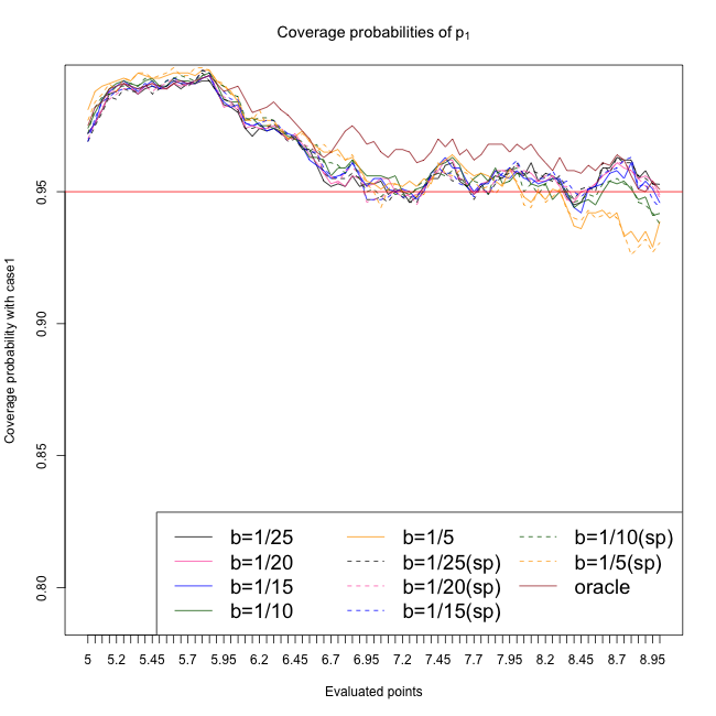
(a) $p_{1}$; C1; $n=500$

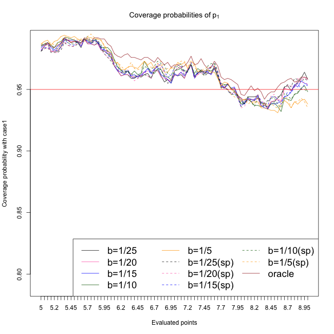
(b) $p_{1}$; C1; $n=1000$

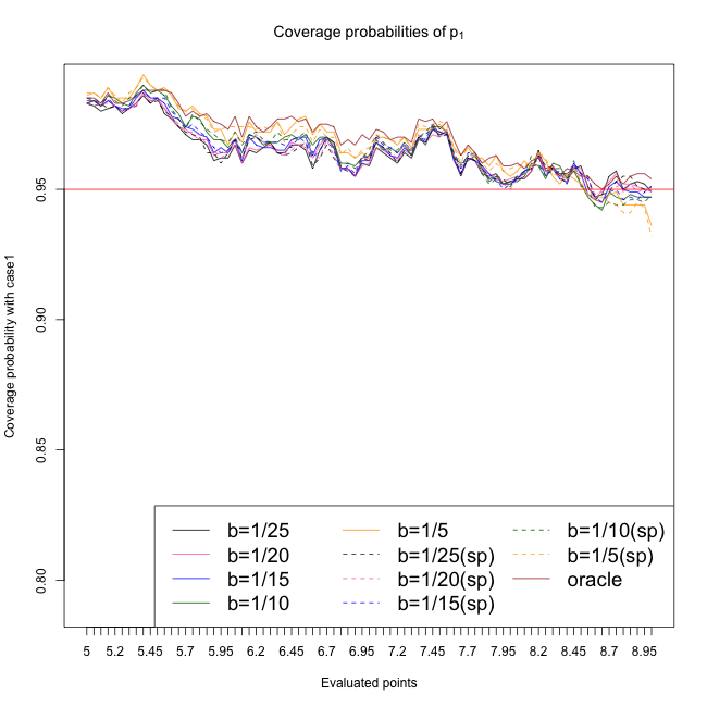
(c) $p_{1}$; C1; $n=2500$

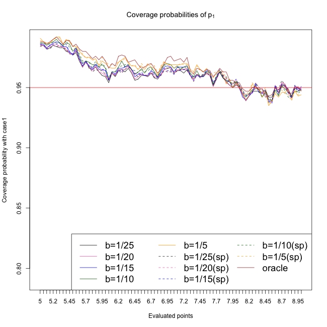
(d) $p_{1}$; C1; $n=4000$

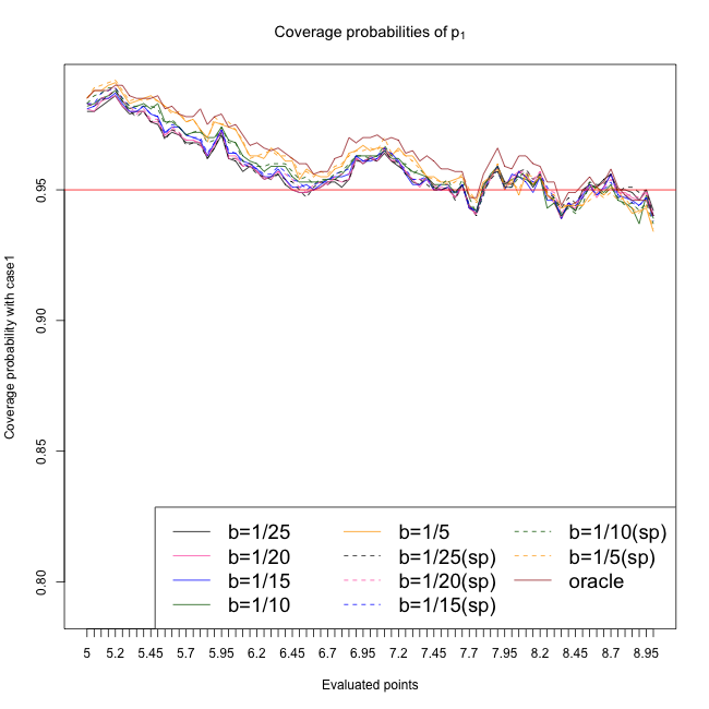
(e) $p_{1}$; C1; $n=6000$

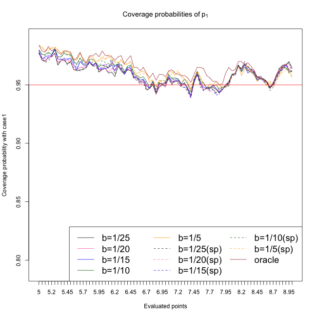
(f) $p_{1}$; C1; $n=8000$

Figure 3: The above displays are coverage probabilities of our proposed log-concave projection estimator’s 95% CIs (labeled as $b=1/m$ where each $b$ means that we used $h_{n}=n^{-b}$ for approximating $\chi_{\theta_{a}}$ (see Section 5.2.1). For the Case 1 where both nuisance functions are well-specified, we also use true value of $\chi_{\theta_{a}}$ to construct the oracle 95% CI which is labeled as oracle in the displays. “sp” stands for our sample splitting based estimator (see (30)). The coverage probabilities are measured in 81 equally spaced points in each domain. Each subcaption describes the estimation target ($p_{1}$ or $p_{0}$), the sample size, and each case of nuisance estimations (Case 1, 2, or 3 abbreviated to C1, C2, and C3, respectively).

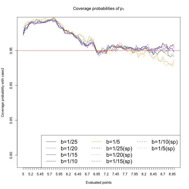
(a) $p_{1}$; C2; $n=500$

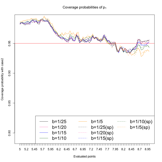
(b) $p_{1}$; C2; $n=1000$

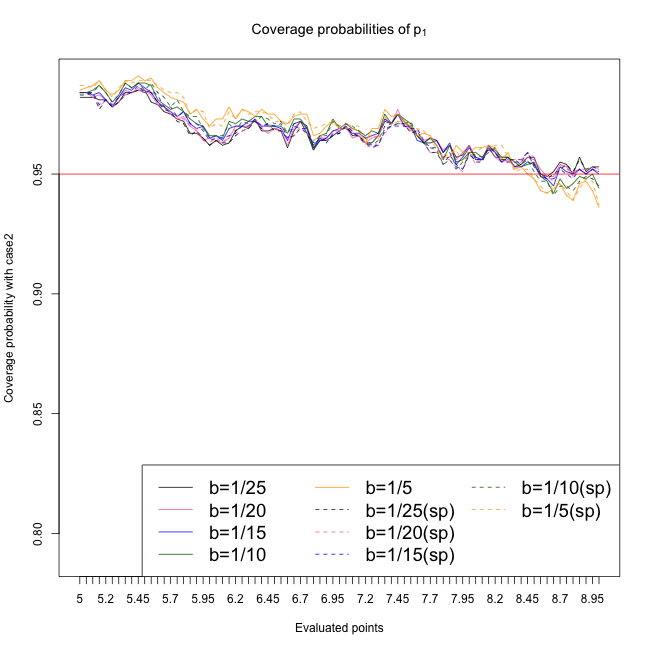
(c) $p_{1}$; C2; $n=2500$

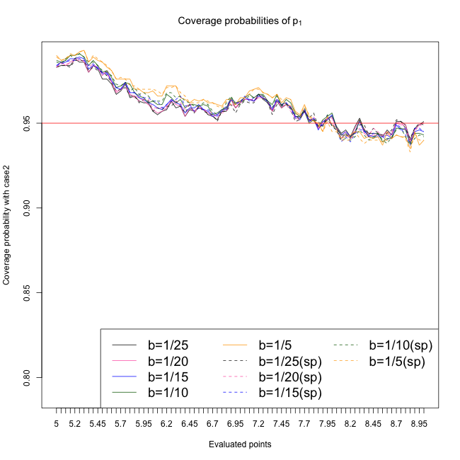
(d) $p_{1}$; C2; $n=4000$

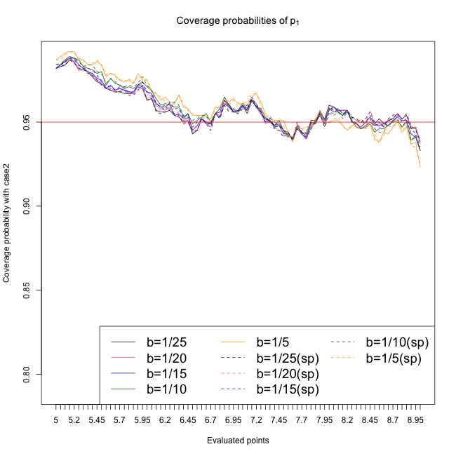
(e) $p_{1}$; C2; $n=6000$

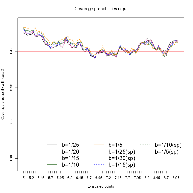
(f) $p_{1}$; C2; $n=8000$

Figure 4: Notational details can be found in Figure 3.

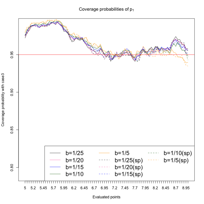
(a) $p_{1}$; C3; $n=500$

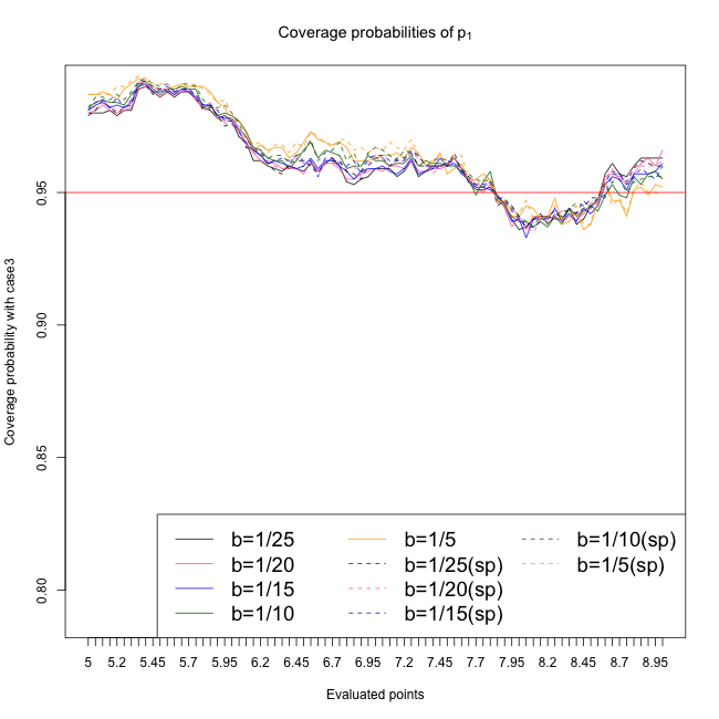
(b) $p_{1}$; C3; $n=1000$

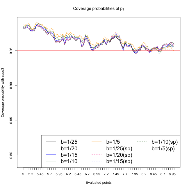
(c) $p_{1}$; C3; $n=2500$

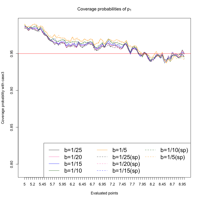
(d) $p_{1}$; C3; $n=4000$

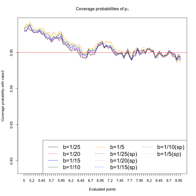
(e) $p_{1}$; C3; $n=6000$

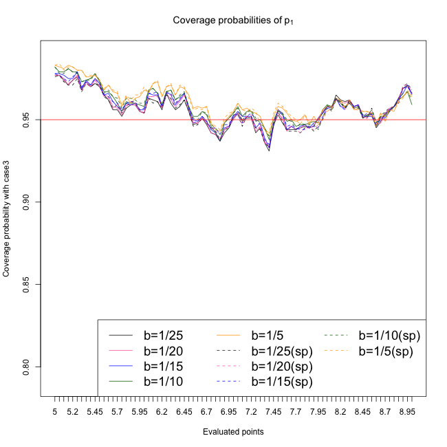
(f) $p_{1}$; C3; $n=8000$

Figure 5: Notational details can be found in Figure 3.

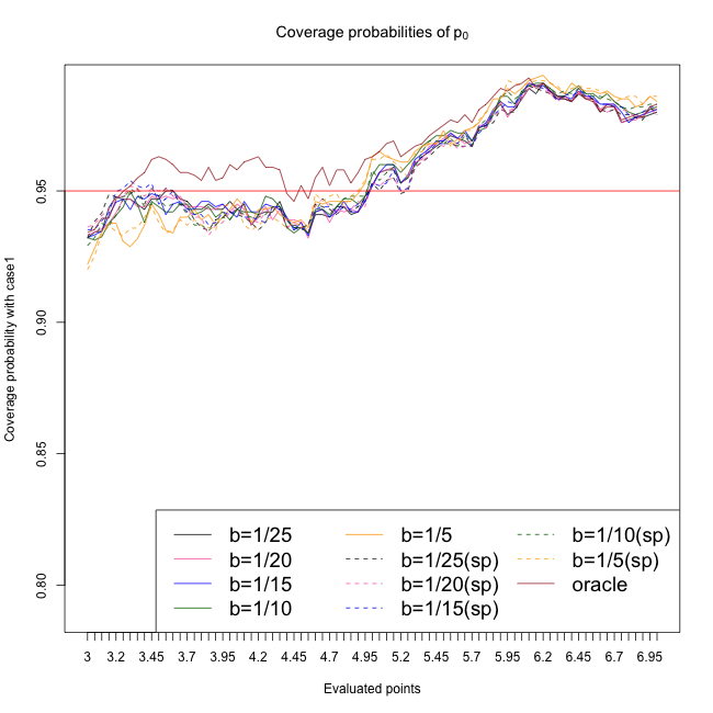
(a) $p_{0}$; C1; $n=500$

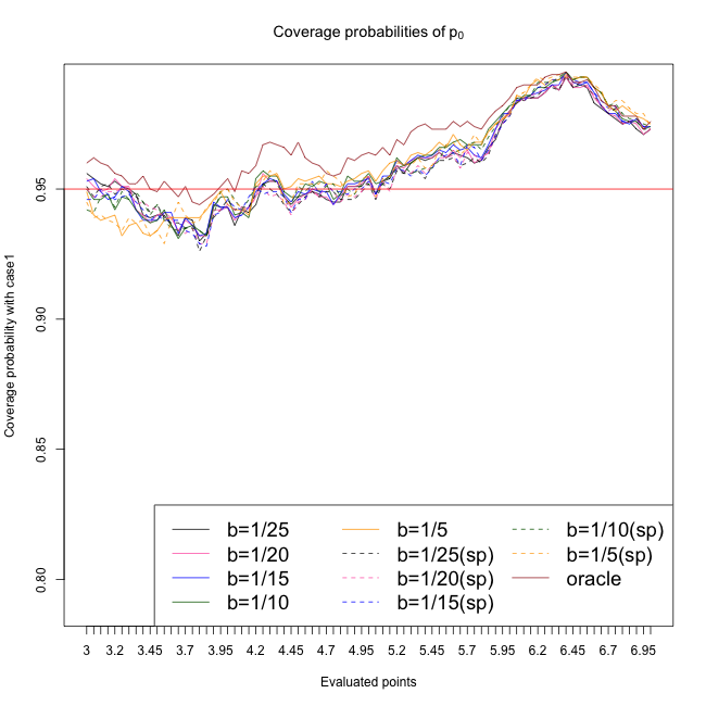
(b) $p_{0}$; C1; $n=1000$

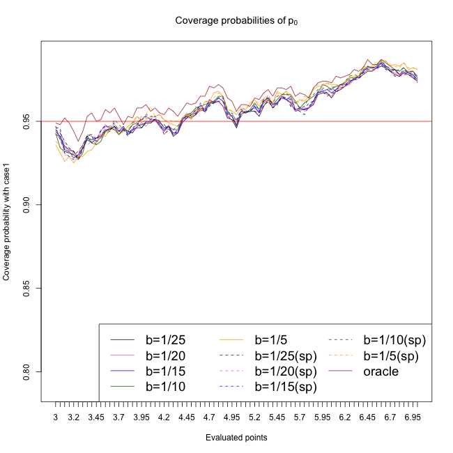
(c) $p_{0}$; C1; $n=2500$

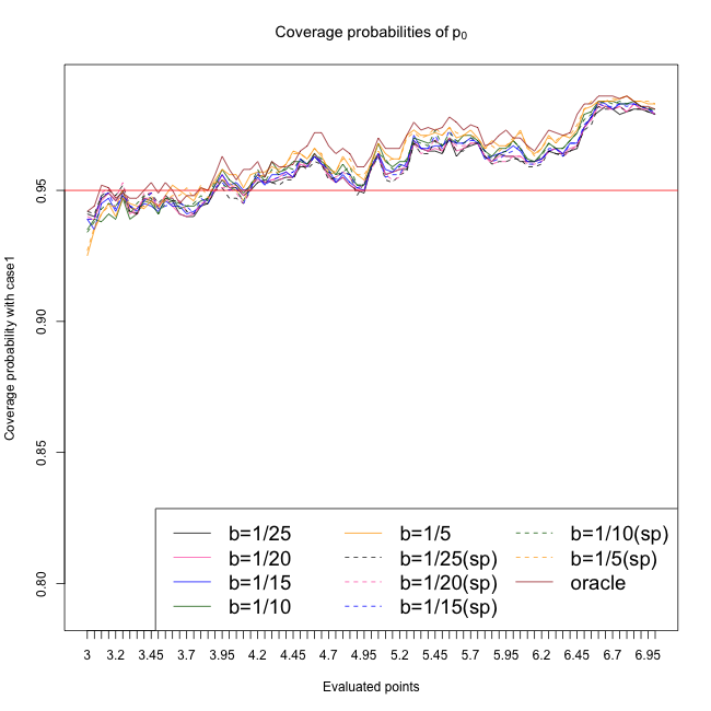
(d) $p_{0}$; C1; $n=4000$

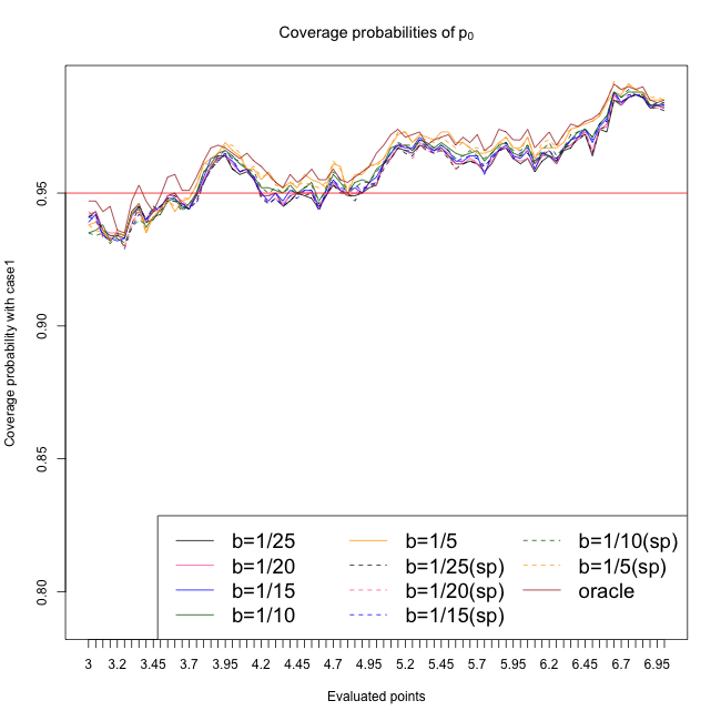
(e) $p_{0}$; C1; $n=6000$

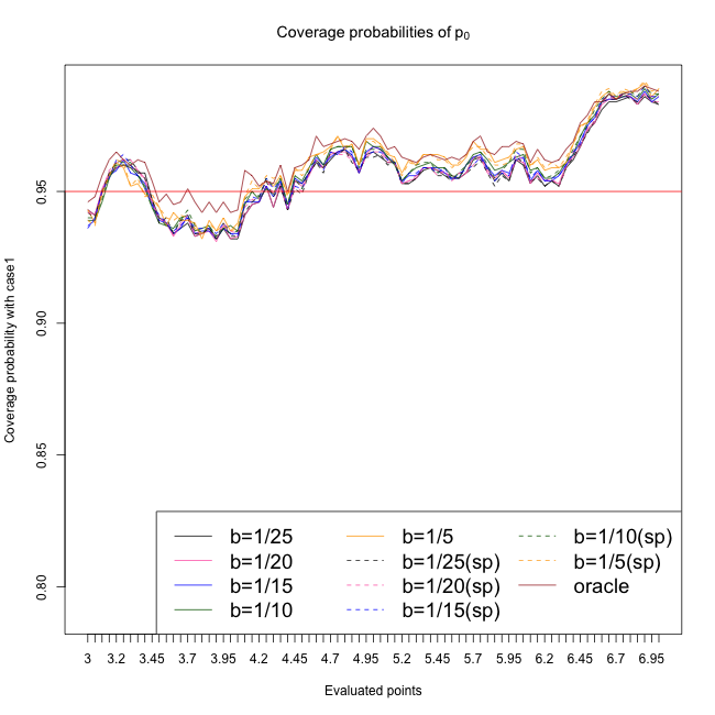
(f) $p_{0}$; C1; $n=8000$

Figure 6: Notational details can be found in Figure 3.

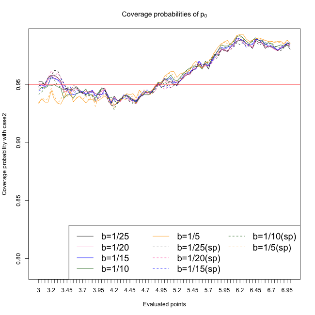
(a) $p_{0}$; C2; $n=500$

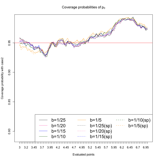
(b) $p_{0}$; C2; $n=1000$

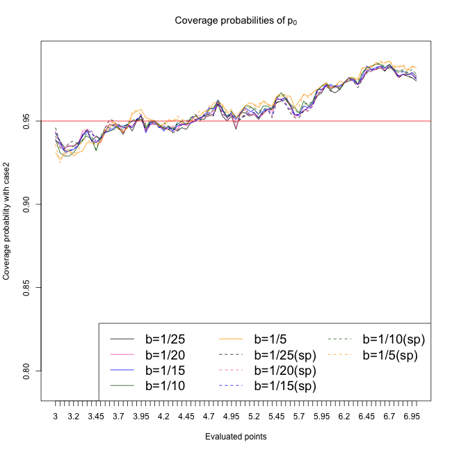
(c) $p_{0}$; C2; $n=2500$

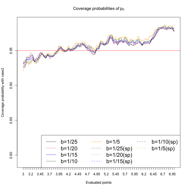
(d) $p_{0}$; C2; $n=4000$

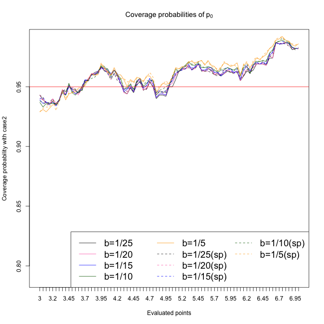
(e) $p_{0}$; C2; $n=6000$

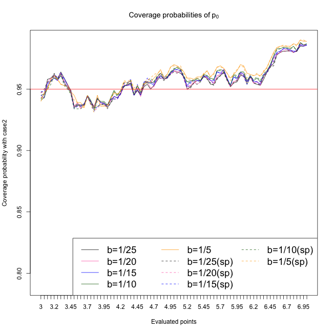
(f) $p_{0}$; C2; $n=8000$

Figure 7: Notational details can be found in Figure 3.

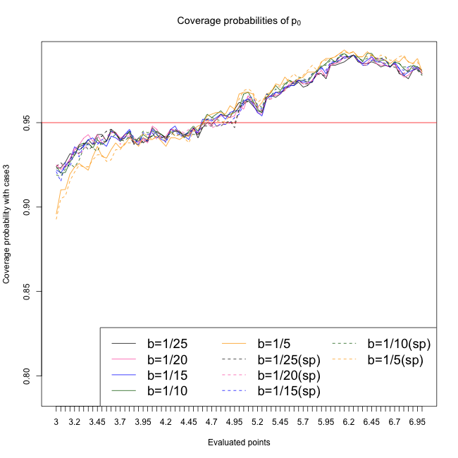
(a) $p_{0}$; C3; $n=500$

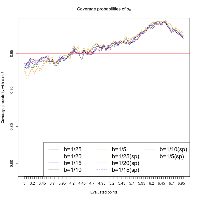
(b) $p_{0}$; C3; $n=1000$

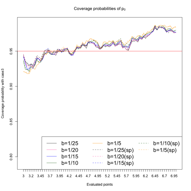
(c) $p_{0}$; C3; $n=2500$

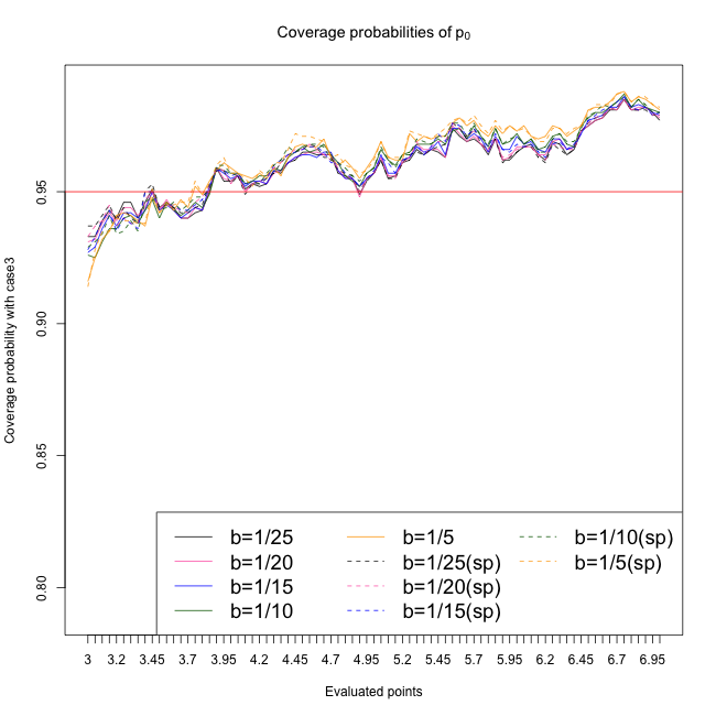
(d) $p_{0}$; C3; $n=4000$

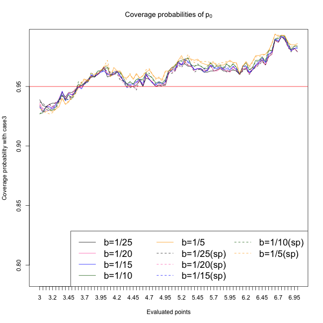
(e) $p_{0}$; C3; $n=6000$

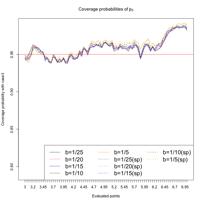
(f) $p_{0}$; C3; $n=8000$

Figure 8: Notational details can be found in Figure 3.

C.4 Additional plots for Section 7

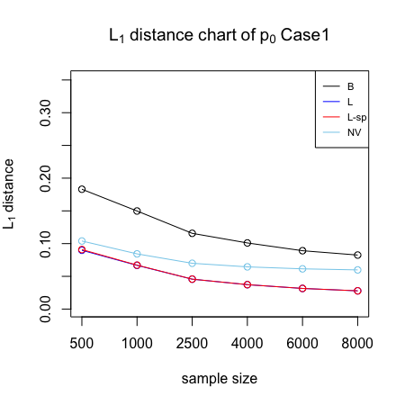
(a) Estimation of $p_{0}$; C1

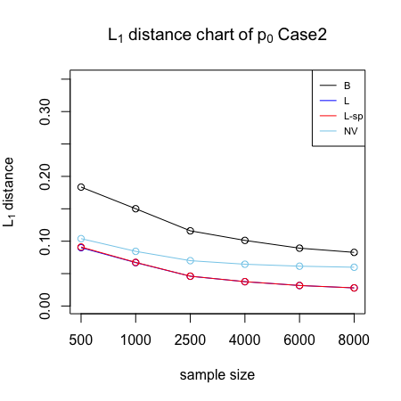
(b) Estimation of $p_{0}$; C2

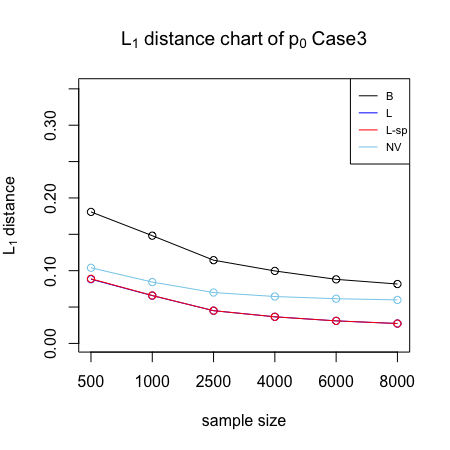
(c) Estimation of $p_{0}$; C3

Figure 9: Average $L_{1}$ distance between the estimators and truth for $p_{0}$. “B”, “L”, and “NV” stand for the basis estimator of Kennedy et al. (2023), the log-concave estimator, and the naive log-concave MLE, respectively. “sp” stands for sample splitting. Case 1 (both nuisance functions well-specified), Case 2 (only the propensity score is well-specified) and Case 3 (only the conditional CDF is well-specified), respectively. The lines for L and L-sp cannot be visually distinguished.

References

- Ayer et al. (1955) Ayer, M., Brunk, H. D., Ewing, G. M., Reid, W. T., and Silverman, E. (1955). An Empirical Distribution Function for Sampling with Incomplete Information. The Annals of Mathematical Statistics 26(4), 641 – 647.
- Balabdaoui et al. (2009) Balabdaoui, F., Rufibach, K., and Wellner, J. A. (2009). Limit distribution theory for maximum likelihood estimation of a log-concave density. The Annals of Statistics 37(3), 1299 – 1331.
- Balabdaoui and Wellner (2007) Balabdaoui, F. and Wellner, J. A. (2007). Estimation of a k-monotone density: Limit distribution theory and the spline connection. The Annals of Statistics 35(6), 2536 – 2564.
- Belloni et al. (2018) Belloni, A., Chernozhukov, V., Chetverikov, D., and Wei, Y. (2018). Uniformly valid post-regularization confidence regions for many functional parameters in z-estimation framework. Annals of statistics 46(6B), 3643.
- Bickel (1982) Bickel, P. J. (1982). On adaptive estimation. The Annals of Statistics 10(3), 647–671.
- Billingsley (2013) Billingsley, P. (2013). Convergence of probability measures. John Wiley & Sons.
- Birgé (1989) Birgé, L. (1989). The Grenander estimator: a nonasymptotic approach. Ann. Stat. 17(4), 1532–1549.
- Chen (2015) Chen, Y. (2015). Semiparametric time series models with log-concave innovations: Maximum likelihood estimation and its consistency. Scandinavian Journal of Statistics 42(1), 1–31.
- Chernozhukov et al. (2018) Chernozhukov, V., Chetverikov, D., Demirer, M., Duflo, E., Hansen, C., Newey, W., and Robins, J. (2018, 01). Double/debiased machine learning for treatment and structural parameters. The Econometrics Journal 21(1), C1–C68.
- Cule and Samworth (2010) Cule, M. and Samworth, R. (2010). Theoretical properties of the log-concave maximum likelihood estimator of a multidimensional density. Electron. J. Stat. 4, 254–270.
- Das and Politis (2019) Das, S. and Politis, D. N. (2019). Nonparametric estimation of the conditional distribution at regression boundary points. The American Statistician.
- Dehejia and Wahba (1999) Dehejia, R. H. and Wahba, S. (1999). Causal effects in nonexperimental studies: Reevaluating the evaluation of training programs. Journal of the American Statistical Association 94(448), 1053–1062.
- Deng et al. (2022) Deng, H., Han, Q., and Sen, B. (2022). Inference for local parameters in convexity constrained models. Journal of the American Statistical Association, 1–15.
- Doss and Wellner (2019a) Doss, C. R. and Wellner, J. A. (2019a). Inference for the mode of a log-concave density. Ann. Statist. 47(5), 2950–2976.
- Doss and Wellner (2019b) Doss, C. R. and Wellner, J. A. (2019b, November). Mode-constrained estimation of a log-concave density.
- Doss and Wellner (2019c) Doss, C. R. and Wellner, J. A. (2019c). Univariate log-concave density estimation with symmetry or modal constraints. Electronic Journal of Statistics 13(2), 2391 – 2461.
- Duembgen et al. (2007) Duembgen, L., Huesler, A., and Rufibach, K. (2007, August). Active Set and EM Algorithms for Log–Concave Densities Based on Complete and Censored Data . pp. 1–26.
- Dümbgen and Rufibach (2009) Dümbgen, L. and Rufibach, K. (2009). Maximum likelihood estimation of a log-concave density and its distribution function: basic properties and uniform consistency. Bernoulli 15(1), 40–68.
- Dümbgen and Rufibach (2011) Dümbgen, L. and Rufibach, K. (2011). logcondens: Computations related to univariate log-concave density estimation. Journal of Statistical Software 39(6), 1–28.
- Dümbgen et al. (2011) Dümbgen, L., Samworth, R., and Schumacher, D. (2011). Approximation by log-concave distributions, with application to regression. The Annals of Statistics 39(2), 702–730.
- Elie-Dit-Cosaque and Maume-Deschamps (2022) Elie-Dit-Cosaque, K. and Maume-Deschamps, V. (2022). Random forest estimation of conditional distribution functions and conditional quantiles. Electronic Journal of Statistics 16(2), 6553–6583.
- Greifer (2023) Greifer, N. (2023). cobalt: Covariate Balance Tables and Plots. R package version 4.5.2.
- Groeneboom and Jongbloed (2014) Groeneboom, P. and Jongbloed, G. (2014). Nonparametric estimation under shape constraints. Number 38. Cambridge University Press.
- Groeneboom et al. (2001a) Groeneboom, P., Jongbloed, G., and Wellner, J. A. (2001a). A canonical process for estimation of convex functions: the “invelope” of integrated Brownian motion . Ann. Statist. 29(6), 1620–1652.
- Groeneboom et al. (2001b) Groeneboom, P., Jongbloed, G., and Wellner, J. A. (2001b). Estimation of a convex function: characterizations and asymptotic theory. Ann. Statist. 29(6), 1653–1698.
- Kennedy (2019) Kennedy, E. H. (2019). Nonparametric causal effects based on incremental propensity score interventions. Journal of the American Statistical Association 114(526), 645–656.
- Kennedy (2023) Kennedy, E. H. (2023). npcausal: Nonparametric causal inference methods. R package version 0.1.0.
- Kennedy et al. (2023) Kennedy, E. H., Balakrishnan, S., and Wasserman, L. A. (2023, 03). Semiparametric counterfactual density estimation. Biometrika. asad017.
- Kim and Pollard (1990) Kim, J. and Pollard, D. (1990). Cube root asymptotics. Ann. Statist. 18(1), 191–219.
- Kim et al. (2018) Kim, K., Kim, J., and Kennedy, E. H. (2018). Causal effects based on distributional distances. arXiv preprint arXiv:1806.02935.
- Kuchibhotla et al. (2023) Kuchibhotla, A. K., Patra, R. K., and Sen, B. (2023). Semiparametric efficiency in convexity constrained single-index model. Journal of the American Statistical Association 118(541), 272–286.
- LaLonde (1986) LaLonde, R. J. (1986). Evaluating the econometric evaluations of training programs with experimental data. The American economic review, 604–620.
- Meinshausen and Ridgeway (2006) Meinshausen, N. and Ridgeway, G. (2006). Quantile regression forests. Journal of machine learning research 7(6).
- Pal et al. (2007) Pal, J. K., Woodroofe, M., and Meyer, M. (2007). Estimating a Polya frequency function2. In Complex datasets and inverse problems, Volume 54 of IMS Lecture Notes Monogr. Ser., pp. 239–249. Beachwood, OH: Inst. Math. Statist.
- Pfanzagl (1982) Pfanzagl, J. (1982). Contributions to A General Asymptotic Statistical Theory. Springer New York, NY.
- Pnanteros et al. (2019) Pnanteros, V. M., Zemel, Y., and Reid, N. (2019). Statistical aspects of wasserstein distances. 6(1), 405–431.
- R Core Team (2022) R Core Team (2022). R: A language and environment for statistical computing.
- Robins (1986) Robins, J. (1986). A new approach to causal inference in mortality studies with a sustained exposure period—application to control of the healthy worker survivor effect. Mathematical modelling 7(9-12), 1393–1512.
- Rubin (1974) Rubin, D. B. (1974). Estimating causal effects of treatments in randomized and nonrandomized studies. Journal of Educational Psychology 66, 688–701.
- Rufibach (2006) Rufibach, K. (2006). Log-concave density estimation and bump hunting for IID observations. Ph. D. thesis, Univ. Bern and Gottingen.
- Rufibach (2007) Rufibach, K. (2007). Computing maximum likelihood estimators of a log-concave density function. J. Stat. Comput. Simul. 77(7-8), 561–574.
- Samworth (2018) Samworth, R. J. (2018). Recent progress in log-concave density estimation. Statistical science 33(4), 493–509.
- Samworth and Yuan (2012) Samworth, R. J. and Yuan, M. (2012). Independent component analysis via nonparametric maximum likelihood estimation. The Annals of Statistics 40(6), 2973 – 3002.
- van der Laan et al. (2011) van der Laan, M. J., Rose, S., Zheng, W., and van der Laan, M. J. (2011). Cross-validated targeted minimum-loss-based estimation. Targeted learning: causal inference for observational and experimental data, 459–474.
- van der Vaart and van der Laan (2006) van der Vaart, A. and van der Laan, M. J. (2006). Estimating a survival distribution with current status data and high-dimensional covariates. The International Journal of Biostatistics 2(1).
- van der Vaart and Wellner (2000) van der Vaart, A. and Wellner, J. A. (2000). Preservation theorems for glivenko-cantelli and uniform glivenko-cantelli classes. In E. Giné, D. M. Mason, and J. A. Wellner (Eds.), High Dimensional Probability II, Boston, MA, pp. 115–133. Birkhäuser Boston.
- van der Vaart and Wellner (1996) van der Vaart, A. W. and Wellner, J. A. (1996). Weak Convergence and Empirical Processes. Springer Series in Statistics. New York: Springer-Verlag.
- Wasserman (2006) Wasserman, L. (2006). All of Nonparametric Statistics. Springer Texts in Statistics. Springer, New York.
- Westling et al. (2020) Westling, T., van der Laan, M. J., and Carone, M. (2020). Correcting an estimator of a multivariate monotone function with isotonic regression. Electronic Journal of Statistics 14(2), 3032 – 3069.
- Whitt (2002) Whitt, W. (2002). Stochastic-process limits: an introduction to stochastic-process limits and their application to queues. Springer.
- Wright and Ziegler (2017) Wright, M. N. and Ziegler, A. (2017). ranger: A fast implementation of random forests for high dimensional data in C++ and R. Journal of Statistical Software 77(1), 1–17.