Fusion Dynamical Systems with Machine Learning in Imitation Learning: A Comprehensive Overview

Abstract

Imitation Learning (IL), also referred to as Learning from Demonstration (LfD), holds significant promise for capturing expert motor skills through efficient imitation, facilitating adept navigation of complex scenarios. A persistent challenge in IL lies in extending generalization from historical demonstrations, enabling the acquisition of new skills without re-teaching. Dynamical system-based IL (DSIL) emerges as a significant subset of IL methodologies, offering the ability to learn trajectories via movement primitives and policy learning based on experiential abstraction. This paper emphasizes the fusion of theoretical paradigms, integrating control theory principles inherent in dynamical systems into IL. This integration notably enhances robustness, adaptability, and convergence in the face of novel scenarios. This survey aims to present a comprehensive overview of DSIL methods, spanning from classical approaches to recent advanced approaches. We categorize DSIL into autonomous dynamical systems and non-autonomous dynamical systems, surveying traditional IL methods with low-dimensional input and advanced deep IL methods with high-dimensional input. Additionally, we present and analyze three main stability methods for IL: Lyapunov stability, contraction theory, and diffeomorphism mapping. Our exploration also extends to popular policy improvement methods for DSIL, encompassing reinforcement learning, deep reinforcement learning, and evolutionary strategies. The primary objective is to expedite readers’ comprehension of dynamical systems’ foundational aspects and capabilities, helping identify practical scenarios and charting potential future directions. By offering insights into the strengths and limitations of dynamical system methods, we aim to foster a deeper understanding among readers. Furthermore, we outline potential extensions and enhancements within the realm of dynamical systems, outlining avenues for further exploration.

1 Introduction

With the growing demand for robotic manipulation tasks, traditional pre-programming methods often face limitations in handling complex scenarios due to the challenges in accurately comprehending and modeling tasks [1]. Over the decades, the field of robotics has experienced significant advancements propelled by progress in high-level artificial intelligence, low-level control theory, decision-making algorithms, and planning techniques [2]. As a result, the robotics community has shifted its focus towards the development of robots capable of imitating expert behaviors. The robots are envisioned to learn and replicate complex natural motor skills, akin to human capabilities. This shift holds promise in simplifying complex tasks and optimizing industrial applications by harnessing expert-level skills through robot reprogramming.

In this vein, LfD arises as a user-friendly and intuitive methodology to teach robots acquiring new tasks. LfD can be broadly categorized into two categories: experience abstraction-based methods and Movement Primitives (MP)-based learning methods [3]. Experience abstraction involves learning new task behaviors by leveraging prior knowledge through policy improvement, where the agent interacts with the environment and updates its policy. Conversely, MP-based learning methods primarily generate continuous control signals derived from DSs.

In practice implementation, demonstrations are collected by human experts and transferred to robots. These demonstrations serve as foundational dataset for generative models that encode motion patterns, empowering robots to perform a diverse range of tasks resembling the demonstrated actions [4].

Demonstrations in Imitation Learning (IL) generally derive from three primary approaches: (i) Kinesthetic teaching [5], (ii) observations [6, 7], and (iii) teleoperation [8, 9]. The selection of an approach depends on the specific scenario at hand and the technological resources available. Kinesthetic teaching involves users manipulating the robot to move as desired and recording trajectories in both joint and Cartesian spaces [10]. The quality of the dataset depends on the smoothness of the user experience. However, this method is limited, especially for certain types of robots, such as legged robots. The observation approach is the passive observation of the user performing a task without the robot’s active participation. This method is suitable for robots with numerous degrees of freedom or non-anthropomorphic designs, as seen in scenarios like collaborative furniture assembly, autonomous driving, and knot tying [11]. Teleoperation involves controlling the robot remotely, often using a master-slave setup or a remote interface. It proves convenient in situations where human intervention is unsafe or impractical [12], such as underwater operations [8] or confined surgical spaces [13]. Nevertheless, its applicability is limited due to the need for specific input interfaces and hardware, such as a joystick, graphical user interface, or force feedback device.

The essence of IL revolves around two key aspects: ensuring the reproduction of demonstrated behaviors and facilitating the model’s ability to adapt to novel scenarios absent from the initial dataset. Selecting the appropriate machine learning algorithm or method for IL is of significant importance. For instance, while some approaches are suitable for large dataset, they might not perform optimally with sparse dataset. Additionally, specific approaches are capable of handling noisy data while still delivering meaningful results. Therefore, the choice of the most suitable approach depends on various factors, including the data nature and the learning objectives. Several machine learning methods have been proposed for IL. These include traditional methods, e.g., DMP [14, 15], GMM and GMR [16, 17, 18], as well as Gaussian Process Regression (GPR), Support Vector Regression (SVR) [19]. Additionally, Hidden Markov Models [20, 21] and Deep Neural Networks [22, 23] have been explored. These methods frequently incorporate principles from control theory or incorporate from control theory or leverage deep learning to improve generalization performance, particularly when dealing with high-dimensional input data.

Several surveys have explored the field of LfD, covering a diverse range of approaches from MP to Reinforcement Learning (RL) or inverse RL. Schaalet al.conducted a survey on artificial intelligence and neural computation in the context of IL, with a particular emphasis on applications for humanoid robots [24]. Their work provided insights into the landscape of IL techniques, emphasizing their relevance in humanoid robotics. Billardet al.contributed to this field through a survey on programming by demonstration or LfD [25]. Their comprehensive survey extensively explored human-robot interaction within LfD, covering a wide spectrum of techniques and methodologies involved in teaching robots tasks through human demonstrations. Additionally, the authors addressed the challenges inherent in this field while discussing potential applications of robot LfD. Argallet al.focused on reviewing the literature related to example state-to-action mappings [26]. Their survey categorized different approaches in terms of demonstration methods, policy derivation, and performance evaluation, across various scenarios. A few years later, Billardet al.addressed general challenges within LfD [27]. They explored fundamental issues such as what to imitate and the evaluation metrics, as well as how to imitate, incorporating aspects like agent motion and force-control tasks. Zhuet al.presented a comprehensive overview of LfD specifically within the context of industrial assembly tasks [28]. Their work spanned various aspects, ranging from the methodology of performing demonstrations to the techniques employed in acquiring manipulation features for IL purposes. Calinon [29] provided a succinct survey on LfD approaches, highlighting key research findings related to data collection, methodology, and application. Xieet al.[30] concentrated on LfD within the domain of robot path planning. Their study highlighted the differences between IL and inverse RL in the context of robot learning. Ravichandaret al.[31] presented an overview of machine-learning approaches for robot learning from experts, including the latest advancements up to 2020, while also addressing practical applications and inherent challenges. Saverianoet al.’s work offered an extensive overview of DMP and various extended versions [15], elucidating their performance, and application conditions, and provided a tutorial for further exploration in this area. Siet al.[32] focused on immersive teleoperation-based IL for manipulation skill learning. The comparison between existing reviews about LfD and our survey is shown in Table 1.

Table 1: Comparison between existing reviews about LfD and our survey.

Survey	Topics	Description
Schaalet al.[24]	• Classical LfD methods • AI and neural computation in LfD • Humanoid Robot	A survey on classical LfD methods that introduces concept of LfD, and its application in humanoid robots. This survey draws connections to mirror neurons and supramodal representation systems and categorizes three major approaches to LfD: learning a control policy, learning from demonstrated trajectories, and model-based LfD.
Billardet al.[25]	• Classical LfD methods • Engineering/Biologically-oriented methods	A survey on classical LfD methods that presents the two main LfD methods: engineering and Biologically oriented methods.
Argallet al.[26]	• Classical LfD methods • Demonstrator: both • Policy derivation	A survey focuses on classical LfD methods, categorizing them into two fundamental phases: gathering demonstration examples from various demonstrators to record data; the second phase centers on deriving a policy by mapping states to actions based on these examples.
Billardet al.[27] & Calinonet al.[29]	• Classical LfD methods • Principle and concept of LfD	These surveys provide an overview of classical LfD methods, introducing the fundamental principles and concepts that underlie LfD approaches, encompassing key components such as demonstrators, classical methodologies, and special functions.
Zhuet al.[28]	• Classical LfD methods • Assembly operations tasks	A survey that introduces the classical LfD methods for assembly tasks.
Xieet al.[30]	• Classical LfD methods • Path planning • RL and Inverse RL	A survey offers a specialized perspective on LfD in the context of path planning. This survey focuses on the classical LfD methods, RL, and inverse RL methods on path planning.
Ravichandaret al.[31]	• General LfD methods • Mature and emerging application	A survey  that conducts an extensive exploration of general LfD methods, encompassing both mature and emerging applications.
Saverianoet al.[15]	• DMP • RL, Deep IL, Lifelong Learning	A survey that provides a comprehensive review and tutorial of DMP, covering various versions of DMP and applications.
Siet al.  [32]	• Classical LfD methods • Demonstrator: teleoperation • Manipulation	A survey that provides an overview of classical LfD methods, with a specific focus on multimodal teleoperation demonstrator-based general LfD techniques for robot manipulation, such as force control.
This paper	• DSIL methods • NDS, ADS • Stability methods • RL, Deep RL, Deep IL • Generalization • Online adaptation	This survey centers on DSIL, categorizing and presenting the evolution of DSIL from classical methods to the latest advancements in deep IL, and RL. Our survey also delves into the essential stability characteristics, spanning from theoretical foundations to published papers.

Figure 1: A taxonomy of existing directions for DS.

Despite the numerous surveys that have extensively covered the broader landscape of LfD methods and their applications, there is a noticeable gap when it comes to Dynamical System-based Imitation Learning (DSIL). Due to the rapid growth of the field, there is a need for a survey to summarize the latest advancements within DSIL. DSIL represents a specialized form of IL, conceptualizing the learning model as a DS, as outlined by Zadeh [33].

Figure 1 illustrates the proposed taxonomy that categorizes existing directions in DSs. DSs encompass a set of differential equations meticulously analyzing the influence of time and force on an agent’s behavior, providing insights into the continuous evolution of agents over time. The left side pertains to Dynamical System-based Control (DSC), where such systems are categorized into two types: linear control systems and nonlinear control systems, or discrete control systems and continuous control systems [34] [35]. In this survey, we specifically concentrate on the DSIL depicted on the right side of Fig. 1. The fusion of control theory principles with DS-based learning models via theory fusion yields enhancements across various facets of system performance, including stability, robustness, and convergence speed. This intersection between control theory and learning systems results in a synergistic effect that magnifies the capabilities of the learning models.

Similar to general IL methods, DSIL can also be classified into two primary categories: MP-based learning methods and experience abstraction-based methods. MP-based methods inherently combine control system principles with machine learning capabilities. This fusion enables the fine-tuning of training parameters, thereby enhancing the model’s robustness and convergence capabilities. On the other hand, experience abstraction-based methods are effectively paired with RL or inverse RL. This integration facilitates the refinement of policy parameters within the DS during interactions with the environment. Consequently, the model acquires adaptability to new tasks, enabling actions such as rejecting perturbations, navigating via points, and avoiding obstacles.

The contributions are summarized as:

• Comprehensive Survey in DSIL: This paper provides a comprehensive survey encompassing 213 papers on the landscape of Dynamical System-based Imitation Learning (DSIL) methods. It covers traditional LfD approaches suitable for low-dimensional inputs as well as the latest advancements in deep LfD tailored for high-dimensional inputs.

• Exploration of Stability Methods in DSIL: The paper extensively analyzes three common stability methods in the context of DSIL. it offers a deep exploration of the theoretical foundations associated with ensuring stability in DSIL.

• Policy Learning Methods in DSIL: This survey thoroughly explores a spectrum of policy learning techniques, encompassing both traditional RL ones and methods grounded in policy learning based on Evolutionary Strategies (ES). Furthermore, it sheds light on the most recent breakthroughs in deep RL methodologies specifically designed to address the nuances of DSIL.

• Research Directions and Challenges in DSIL: Beyond providing an overview of the existing landscape and methodologies, this paper identifies and outlines the key research directions. It also discusses current challenges and open problems in DSIL.

Our exploration spans both theoretical advancements and practical applications within the realm of DSIL.

The rest of this survey is organized as follows: Section 2 introduces two types of DSs: autonomous and non-autonomous, contextualizing their roles within IL. Section 3 covers three common stability approaches employed in DSIL, offering insights into ensuring stability within DSIL. Section 4 discusses existing policy learning methods, including RL, ES, and deep RL, among others. In Section 5, we introduce deep IL with high-dimensional input. In Section 7, we discuss challenges and future directions on DSIL. Finally, our survey is concluded in Section 8.

2 MP learning with low dimension input

Table 2: Description of key abbreviations.

IL	Imitation Learning	RL	Reinforcement Learning
LWR	Locally Weighted Regression	DMP	Dynamic Movement Primitive
GMM	Gaussian Mixture Model	GMR	Gaussian Mixture Regression
DoF	Degree of Freedom	GPR	Gaussian Process Regression
SVR	Support Vector Regression	HMM	Hidden Markov Model
DNN	Deep Neural Network	DSIL	Dynamical System-based Imitation Learning
ADSIL	Autonomous Dynamical Systems-based Imitation Learning	NDSIL	Non-autonomous Dynamical Systems-based Imitation Learning
ProMP	Probabilistic Movement Primitives	MP	Movement Primitives
APF	Artificial Potential Field	MPC	Model Predictive Control
EKF	Extended Kalman Filter	EM	Expectation Maximization
HSMM	Hidden Semi-Markov Model	ADHSMM	adaptive duration
PI2	Policy Improvement with Path Integrals	CMA-ES	Covariance Matrix Adaptation Evolution Strategy
MPG	Motor Primitive Generalization	SEDS	Stable Estimator of Dynamical Systems
FSM-DS	Fast and Stable Modeling for Dynamical Systems	CLF-DM	Control Lyapunov Function-based Dynamic Movements
WSAQF	Weighted Sum of Asymmetric Quadratic Function	PC-GMM	Physically Consistent-
C-GMR	contracting-	ESDS	Energy-based Stabilizer of Dynamical Systems
PCA	Principal Component Analysis	K-PCA	Kernel
BLS	Broad Learning System	QLF	Quadratic Lyapunov Function
LTL	Linear Temporal Logic	SOS-CLF	Sum Of Squares-control Lyapunov Functions
NS-QLF	Neural Shaped-	ICNN	Input Convex Neural Network
PLYDS	PoLYnomial Dynamical System	LSD-IQP	Learning Stable Dynamical systems with Iterative Quadratic Programming
CT	Contraction Theory	CVF	Contracting Vector Fields
CDSP	Continuous Dynamical Systems Prior	CCM	Control Contraction Metrics
NCM	Neural Contraction Metrics	SDS-EF	Stable Dynamical System learning using Euclideanizing Flows
SDE	Stochastic Differential Equation	FAGIL	Fail-Safe Adversarial Generative Imitation Learning
DT	Diffeomorphic Transform	RSDS	Riemannian Stable Dynamical Systems
ODE	Ordinary Differential Equation	PoWER	Policy learning by Weighting Exploration with the Returns
eNAC	episodic Natural Actor Critic	MMT	Model Mediated Teleoperation
ELM	Extreme Learning Machine	NES	Natural Evolution Strategies
ES	Evolutionary Strategies	xNES	Exponential
TR-CMA-ES	Trust-Region CMA-ES	DDPG	Deep Deterministic Policy Gradient
NNMP	Neural Network-based Movement Primitive	SAC	Soft Actor-Critic
ORB	Optimal Replay Buffer	rLfD	residual
PPO	Proximal Policy Optimization	CPG	Central Pattern Generators
VPG	Vanilla Policy Gradient	CrKR	Cost-regularized Kernel Regression
HiREPS	Hierarchical Relative Entropy Policy Search	MLP	Multi-Layer Perceptron
CNN	Convolutional Neural Network	TP-DMP	Trajectory Parameterized-
IMEDNet	Image-to-Motion Encoder-Decoder Networks	CIMEDNet	Convolutional
STIMEDNet	spatial transformer	RNN	Recurrent Neural Networks
DSDNet	Deep Segmented Networks	AL-DMP	Arc Length-
VIMEDNet	Variable	NDPs	Neural Dynamic Policies
H-NDP	Hierarchical	LF	Lyapunov Function
P-QLF	Parameterize-	RBFNN	Radial Basis Function Neural Network
DAgger	Data Aggregation Approach	LLM	Large Language Model
CLF	Control Lyapunov Function	CBF	Control Barrier Function
BBO	Black-Box Optimization	VSDS	Variable Stiffness Dynamical System

Table 3: Description of key notations.

$K$	$\triangleq$	# of basis/Gaussian function	$k$	$\triangleq$	index $:k=1,2,\ldots,K$
$\mathcal{O}$	$\triangleq$	# of demonstrations	$o$	$\triangleq$	index $:o=1,2,\ldots,\mathcal{O}$
$N$	$\triangleq$	# of trajectory length	$n$	$\triangleq$	index $:n=1,2,\ldots,N$
$\mathcal{I}$	$\triangleq$	# of samples in exploration	$i$	$\triangleq$	index $:i=1,2,\ldots,\mathcal{I}$
$\tau$	$\triangleq$	# time modulation parameter	$c_{k},\omega_{k}$	$\triangleq$	centers and widths of Gaussian
$\alpha_{z},\beta_{z},\alpha_{\xi}$	$\triangleq$	positive gain	$T_{p}$	$\triangleq$	rotation matrix
$\eta_{p},\mu_{1},\mu_{2},\mu_{3},A_{p}$	$\triangleq$	positive gain	$l_{1},l_{2},l_{3}$	$\triangleq$	axis length of $C_{p}$
$\rho$	$\triangleq$	positive gain	$x_{1},x_{2},x_{3}$	$\triangleq$	centers of $C_{p}$
$\kappa$	$\triangleq$	adjusted parameter	$\eta_{l}$	$\triangleq$	learning rate
$\xi$	$\triangleq$	decay phase variable	$x,\dot{x},\ddot{x}$	$\triangleq$	trajectory data
$C_{p}$	$\triangleq$	obstacle function	$U(x,\dot{x})$	$\triangleq$	potential field function
$f(x),f(x,t)$	$\triangleq$	dynamical system function	$G(x,\dot{x})$	$\triangleq$	repulsive force function
$\theta$	$\triangleq$	learnable parameters	$\vartheta$	$\triangleq$	angle between two vectors
$x^{*}$	$\triangleq$	goal position	${\varphi_{i}}$	$\triangleq$	basis function
$q$, $q_{r}$ and $\dot{q}$, ${\dot{q}}_{r}$	$\triangleq$	actual and desired joint angle , its 1st time-derivative	$z,\dot{z}$	$\triangleq$	scaled velocity and acceleration
$f_{\xi,\theta}$, $f_{\xi}$	$\triangleq$	forcing term for different spaces	$h_{i}$	$\triangleq$	weights
$p(k)$, $p(x|k)$	$\triangleq$	prior probability and conditional Probability	$R$	$\triangleq$	parameter matrix
$\mu_{k}^{\dot{x}}$, $\mu_{k}^{x}$, $\mu_{\theta}$	$\triangleq$	mean	$Dis(x)$	$\triangleq$	distance between robot and obstacles
$\Sigma_{k}^{x}$, $\Sigma_{k}^{\dot{x}x}$, ${\Sigma_{\theta}}$	$\triangleq$	covariance	$V(x)$, ${\tilde{V}}(x)$	$\triangleq$	Lyapunov function
$\varpi$	$\triangleq$	weight of $\rm{PI}^{2}$	$u_{t_{j}}$, $u$, ${u_{f\omega}}$	$\triangleq$	control input
$\delta_{x}$, $\dot{\delta}_{x}$	$\triangleq$	virtual displacement, its 1st time-derivative	$\mathcal{M}$	$\triangleq$	a Riemannian manifold
$J$, $J_{\Psi}$	$\triangleq$	Jacobian matrix	$\psi$	$\triangleq$	diffeomorphism mapping
$\hbar$	$\triangleq$	coordinate transformation output	$S$, $\bar{S}$	$\triangleq$	cost function
$\phi_{{t_{N}}}$, $\gamma_{{t_{i}}}$	$\triangleq$	terminal and immediate cost	$\lambda\left(x\right)$	$\triangleq$	eigen values
$P$	$\triangleq$	positive define matrix	$Q$, $H$	$\triangleq$	negative define matrix
$\mathbb{J}$	$\triangleq$	expected cost	$\varepsilon_{t}$, $\varepsilon_{k,t}$	$\triangleq$	exploration noise
${\nu_{i}}$	$\triangleq$	utilities function	$r\left({{\theta_{i}}}\right)$	$\triangleq$	reward
$\Phi$, ${\Phi_{k,t}}$	$\triangleq$	control matrix	$\nabla$	$\triangleq$	gradient
$L_{i}$	$\triangleq$	i-th sample trajectory of $\rm{PI}^{2}$	$F$	$\triangleq$	Fisher matrix
$K^{p}$	$\triangleq$	stiffness gains	$K^{v}$	$\triangleq$	damping gains

MP can be categorized into two main types: (a) Dynamics-based approaches: These methods are capable of generating smooth trajectories from any given initial state. A notable example of this type is DMP [36]. (b) Probabilistic approaches: This category focuses on capturing higher-order statistics of motion. An example within this category is Probabilistic Movement Primitives (ProMP) [37]. These two categories offer distinct approaches for modeling and generating movements, each with its strengths and applications.

This section introduces an overview of MP-based DS learning focusing on low-dimensional input. In [38], the authors categorized MP learning methods into two categories: autonomous and non-autonomous systems. Non-autonomous Dynamical Systems-based Imitation Learning (NDSIL) is a field that deals with the imitation and control of systems whose behavior evolves, over time, in response to external inputs or forces. NDSIL depends on time-varying factors or control inputs to drive their trajectories.

1. Time-dependent behavior: NDSIL deals with systems whose behavior is influenced by external factors or control inputs, adding complexity to modeling and imitation. This time-dependent aspect requires sophisticated approaches to accurately replicate and predict behaviors that evolve over time.

2. Generalization: in NDSIL, LfD involves capturing not only the nominal behavior but also the variations induced by external inputs. Robust generalization in NDSIL demands a broader understanding of how diverse external factors affect system behavior, enhancing adaptability and performance in varied scenarios.

The distinctions between autonomous and non-autonomous DS lie primarily in how they evolve over time and the factors that influence their behavior, Table 4.

Table 4: Autonomous DS vs. non-autonomous DS.

Autonomous DS	Non-autonomous DS
The evolution of the system depends solely on its current state. There are no external inputs or time-varying parameters that directly influence the system’s dynamics, e.g., equation (1)	The evolution of the system depends not only on its current state but also on external inputs or time-varying parameters that directly influence its dynamics, e.g., equation (2)
They are often characterized by fixed equations of motion that describe how the system evolves over time.	They are often characterized by equations of motion that explicitly include time-varying terms or external inputs.
Examples include simple mechanical systems like pendulums, as well as more complex systems like autonomous vehicles navigating without external control.	Examples include systems subjected to time-varying external forces, such as robots controlled by external commands or systems influenced by environmental factors that change over time.

$$\dot{x} =f(x)$$ (1)

$$\dot{x} =f(x,t)$$ (2)

These MP models, described by (1) and (2), facilitate the generation of motion sequences, incorporating an initial state as part of their functionality. This allows the prediction or simulation of behaviors based on the specified starting conditions. For a better understanding, we have summarized the used abbreviations and the key notations in Tables 2 and 3.

In the following subsections, we begin by introducing the NDSIL methods. Subsequently, we present the Autonomous Dynamical Systems-based Imitation Learning (ADSIL) methods.

2.1 Non-autonomous Dynamical Systems-based Imitation Learning (NDSIL)

The evolution of non-autonomous systems relies on external variables beyond the system state. One of the classical methods of NDSIL is the DMPs which was initially developed by Ijspeertet al.in 2002 [36] and further refined in 2013 [14].

The DMP framework is a straightforward damped spring model coupled with a forcing function to learn trajectories. The damped spring model attracts the robot towards a defined goal position, while the forcing function guides the robot to follow a given trajectory. Consequently, it exhibits a property of globally converging towards a goal position from any initial position. The concept behind DMP involves envisioning complex movements as compositions of sequential or simultaneous primitive movements. Consequently, DMP is capable of imitating demonstrations and reproducing similar motions, particularly for point-to-point trajectories or periodic trajectories. Moreover, advancements in DMP extend its capabilities to encode the orientation [39, 40, 41, 42, 43, 44] and Symmetric Positive Definite (SPD) [45] trajectories, facilitating continuous transitions between successive motion primitives. Interested readers can refer to [15] for a more comprehensive survey with various formulations and extensions of DMPs.

The basic formulation of a single DMP is defined as:

$$\tau\dot{z} =\alpha_{z}\left(\beta_{z}(x^{*}-x)-z\right)+f_{\xi,\theta}(\xi,\theta)$$ (3)

$$\tau\dot{x} =z$$ (4)

$$\tau\dot{\xi} =-\alpha_{\xi}\xi$$ (5)

$$f_{\xi,\theta}\left(\xi,\theta\right) =\frac{{\sum\nolimits_{k=1}^{K}{{\theta_{k}}{\varphi_{k}}(\xi)}}}{{\sum\nolimits_{k=1}^{K}{{\varphi_{k}}(\xi)}}}\xi$$ (6)

$${\varphi_{k}}(\xi) =\exp\left({-{\omega_{k}}{{(\xi-{c_{k}})}^{2}}}\right)$$ (7)

where Eqs. (3) and (4) are transformation system, Eq. (5) is the canonical system, Eq. (6) is the forcing term, and Eq. (7) is the Gaussian kernel. The parameters $\tau$, $\alpha_{z}$, $\beta_{z}$, $\alpha_{\xi}$ are positive constant and $\theta$ is the shape parameter which is used for training. $x^{*}$ is the goal position of the DS. Indeed, DMP represents a time-dependent DS. The performance of NDSIL utilizing DMP on the LASA dataset [18] is illustrated in Fig. 2.

Figure 2: The imitation performance of NDSIL utilizing DMP is evaluated on a dataset containing 20 instances of human handwriting motions. The black ‘$\cdot$’ and ‘*’ symbols denote the initial and goal points, respectively. The blue dashed line represents the demonstration, while the solid brown line illustrates the reproduced imitation.

Table 5: Different potential functions for obstacle avoidance of NDSIL. $Dis(x)$ is the distance between robot and obstacles; $Dis_{0}$ is the threshold value; $\eta_{p}$, $\mu_{1}$, $\mu_{2}$, $\mu_{3}$ and $A_{p}$ are constant parameters.

Methods	Repulsive functions	Auxiliary function
Point-steering [46]	$G\left({x,\dot{x}}\right)=\eta_{p}T_{p}\dot{x}\vartheta\exp\left({-\mu_{1}\vartheta}\right)$	$\vartheta=\arccos\left({\frac{{\left\langle{o-x,\dot{x}}\right\rangle}}{{\left\|{o-x}\right\|\left\|{\dot{x}}\right\|}}}\right)$
Point-static [47, 48]	$G\left({x,\dot{x}}\right)=-{\nabla_{x}}U\left({x,\dot{x}}\right)$	$U\left({x,\dot{x}}\right)=\left\{\begin{array}[]{l}\frac{\eta_{p}}{2}{\left({\frac{1}{{Dis(x)}}-\frac{1}{{Dis_{0}}}}\right)^{2}}~{}~{}Dis(x)\leq{Dis_{0}}\\ 0{\rm{~{}~{}~{}~{}~{}~{}~{}~{}~{}~{}~{}~{}~{}~{}~{}~{}~{}~{}~{}~{}~{}~{}}}Dis(x)>Di{s_{0}}\end{array}\right.$
Point-dynamic [49]	$G\left({x,\dot{x}}\right)=-{\nabla_{x}}U\left({x,\dot{x}}\right)$	$U\left({x,\dot{x}}\right)=\left\{{\begin{array}[]{*{20}{l}}{{\eta_{p}}{{\left({-\cos\vartheta}\right)}^{{\mu_{1}}}}\frac{{\left\|{\dot{x}}\right\|}}{{Dis(x)}}\;\;\;\;\;{\rm{if}}\;\;\vartheta\in\left({\frac{\pi}{2},\pi}\right]}\\ {0\;\;\;\;\;\;\;\;\;\;\;\;\;\;\;\;\;\;\;\;\;\;\;\;\;\;\;\;\;\;{\rm{if}}\;\;\vartheta\in\left[{0,\frac{\pi}{2}}\right)}\end{array}}\right.$
		$\cos\vartheta=\frac{{\left\langle{\dot{x},x-o}\right\rangle}}{{\left\|{x-o}\right\|\left\|{\dot{x}}\right\|}}$
Volume-static [48]	$G\left({x,\dot{x}}\right)=-{\nabla_{x}}U\left({x,\dot{x}}\right)$	$U\left({x,\dot{x}}\right)=\frac{{A_{p}\exp\left({-\eta_{p}C_{p}(x)}\right)}}{{C_{p}(x)}}$
		$C_{p}(x)={\left({\frac{{{x_{1}}-{{\hat{x}}_{1}}}}{{{l_{1}}}}}\right)^{2{\mu_{1}}}}+{\left({\frac{{{x_{2}}-{{\hat{x}}_{2}}}}{{{l_{2}}}}}\right)^{2{\mu_{2}}}}+{\left({\frac{{{x_{3}}-{{\hat{x}}_{3}}}}{{{l_{3}}}}}\right)^{2{\mu_{3}}}}-1$
Volume-dynamic [50]	$G\left({x,\dot{x}}\right)=-{\nabla_{x}}U\left({x,\dot{x}}\right)$	$U\left({x,\dot{x}}\right)=\left\{\begin{array}[]{l}\eta_{p}{\left({-\cos\vartheta}\right)^{{\mu_{1}}}}\frac{{\left\|{\dot{x}}\right\|}}{{{C^{{\mu_{2}}}}(x)}}{\rm{~{}~{}~{}if}}~{}~{}\vartheta\in\left({\frac{\pi}{2},\pi}\right]\\ 0{\rm{~{}~{}~{}~{}~{}~{}~{}~{}\;~{}~{}~{}~{}~{}~{}~{}~{}~{}~{}~{}~{}~{}~{}~{}if}}~{}~{}\vartheta\in\left[{0,\frac{\pi}{2}}\right)\end{array}\right.$
		$C_{p}(x)={\left({{{\left({\frac{{{x_{1}}-{{\hat{x}}_{1}}}}{{{l_{1}}}}}\right)}^{2{\mu_{1}}}}+{{\left({\frac{{{x_{2}}-{{\hat{x}}_{2}}}}{{{l_{2}}}}}\right)}^{2{\mu_{1}}}}}\right)^{\frac{{2{\mu_{2}}}}{{2{\mu_{1}}}}}}+{\left({\frac{{{x_{3}}-{{\hat{x}}_{3}}}}{{{l_{3}}}}}\right)^{2{\mu_{2}}}}-1$

In order to enhance the generalization performance of NDSIL, various methods have incorporated a steering angle term into the DS after training, aiming to avoid obstacles in new environment [46, 51, 52, 53]. However, this Point-steering solely relies on the steering angle without considering the distance between the robot and obstacles. Consequently, it might lead to oscillatory behaviors due to the absence of distance-based adjustments. Similarly, in the Point-static method, the Artificial Potential Field (APF) has been employed within NDSIL of DMP [52]. This method utilizes global convergence as an attraction force and calculates the repulsion force between the robot and obstacles based on potential functions. However, due to the absence of velocity information, there might be a tendency for non-smooth behaviors when encountering obstacles. Parket al.[49] proposed an improved potential function that incorporates both distance and velocity information known as the Point-dynamic method. However, methods like [46] and [49] are point obstacle types, necessitating the calculation of information between the robot and surface point clouds of objects, resulting in a high computation burden for large volume obstacles. Addressing obstacles as entire volumes, Ginesiet al.[48] proposed a Volume-static method, modeling obstacles as convex 3D shapes., They introduced a Volume-based potential function, improving real-time performance. Nonetheless, similar to the "Point-static method", the work in [48] does not involve velocity information, potentially encountering analogous issues. In their subsequent work, Ginesiet al.[50] proposed the Volume-dynamic method, which integrates both volumes and velocity information into the potential function. Table 5 summarizes these five methods for reference.

In [54] and [55], Kruget al.introduced a Model Predictive Control (MPC) approach for NDSIL using DMP. This approach aims to generate predictive optimal motion plans with a planning horizon of $P$-steps. This allows for real-time updates of trajectory generation at each time step, facilitating obstacle integration through constraints within the MPC, while adhering to spatial and temporal polyhedral constraints. Another strategy addressing obstacles involves extending the DS formulation with a repulsive function, similar to the one represented in (8) [56]. This extension aims to incorporate obstacle avoidance directly within the DS formulation.

In [54] and [55], Kruget al.introduced a MPC approach for NDSIL using DMP. This approach aims to generate predictive optimal motion plans with a planning horizon of $P$-steps. This allows for real-time updates of trajectory generation at each time step, facilitating obstacle integration through constraints within the MPC, while adhering to spatial and temporal polyhedral constraints. Another strategy addressing obstacles involves extending the DS formulation with a repulsive function, similar to the one represented in (8) [56]. This extension aims to incorporate obstacle avoidance directly within the DS formulation.

The formulation for obstacle avoidance within NDSIL is presented as:

$$\ddot{x}{\rm{}}=\underbrace{f\left({x,\dot{x},t}\right)}_{{\rm{attraction}}\;{\rm{force}}}+\underbrace{G\left({x,\dot{x}}\right)}_{{\rm{repulsive}}\;{\rm{force}}}$$ (8)

where the attraction force $f\left({x,\dot{x},t}\right)$ embodies the trained stable DS, akin to (3) and (4). Meanwhile, the additional term $G\left({x,\dot{x}}\right)$ represents the repulsive force designed for obstacle avoidance. The formulation outlines five different potential functions, detailed in Table 5. The properties of various methods for obstacle avoidance are summarized in Table 6. The first method, Point-steering, solely calculates the steering angle for obstacle avoidance without accounting for distance, which can lead to larger errors. Additionally, the Point-steering, Point-static, and Point-dynamic methods compute the repulsion force point-by-point using a 3D point cloud of obstacles, resulting in computational burden compared to volume methods. The Point-static and Volume-static methods only support static obstacles as they do not incorporate velocity information. Acceleration and error characteristics are depicted in Fig. 3. Although the Point-static, Point-dynamic, Volume-static, and Volume-dynamic methods are not guaranteed to converge to the goal due to the possibility of local minima, a perturbation term can be easily added to push the DS out of local minima. The comparative performance evaluation of these methods is illustrated in Fig. 3.

Table 6: The properties of various methods for obstacle avoidance [50].

Methods	Obstacle type	Potential type	Distance dependent	Guaranteed convergence
Point-steering	point	dynamic	No	Yes
Point-static	point	static	Yes	No
Point-dynamic	point	dynamic	Yes	No
Volume-static	volume	static	Yes	No
Volume-dynamic	volume	dynamic	Yes	No

Figure 3: Different potential functions obstacle avoidance performance of NDSIL in DMP [50].

Generally, non-autonomous movement representations fundamentally establish a direct relationship between a temporal signal and the dynamic attributes of the motion. The retrieval of movement from such models relies heavily on this temporal signal, which might directly signify time or employ an indirect representation through a decay term. In addition to the DMP methods of IL, we are exploring other classical NDSIL learning methods. These approaches offer diverse perspectives and methodologies in capturing and replicating dynamic behaviors.

In several studies [57, 58, 59, 60, 16, 61], the problem of learning DS has been reformulated using GMR or HMM. Unlike DMPs, this methodology allows for encoding multiple demonstrations.

$$\ddot{x} =\sum\limits_{k=1}^{K}{{h_{k}}(t)\left[{K_{k}^{p}(\mu_{k}^{x}-x)-{K^{v}}\dot{x}}\right]}$$ (9)

$${h_{k}}\left(t\right) =\frac{{\mathcal{N}\left({t;\mu_{k}^{t},\Sigma_{k}^{t}}\right)}}{{\sum\nolimits_{j=1}^{K}{\mathcal{N}\left({t;\mu_{j}^{t},\Sigma_{j}^{t}}\right)}}}$$

where $K_{k}^{p}$, $K^{v}$, and $\mu_{k}^{x}$ denote the full stiffness matrix, damping term, and attractor point, respectively, of the $k$-th virtual spring. Equation (9) shares a structural similarity with DMPs. However, it is important to note that the weight parameter $h_{k}$ assumes distinct interpretations in the contexts of DMPs and Eq. (9). In DMP, the determination of these weights ($h_{k}$) relies on the decay term $\xi$ as defined in the system dynamics (5). These weights are inherently embedded within the GMR/HMM representation of the motion. This alternative approach offers several advantages over DMP: (i) It provides enhanced flexibility in addressing spatial and temporal distortions. (ii) Skill training and refinement are accomplished using partial demonstrations. (iii) Learning tasks involving reaching and cyclic motions become feasible without predefined dynamics.

In [62], Calinonet al.exploited HSMMs within IL for non-autonomous systems. This focuses on integrating temporal and spatial constraints, emphasizing adaptability in the face of perturbations. Gribovskayaet al.[63] proposed an innovative method for learning discrete bimanual coordination skills. This method integrates the automated extraction of spatio-temporal coordination constraints with a resilient motor system capable of generating coordinated movements. It operates effectively even in the presence of perturbations while adhering to learned coordination constraints. Forteet al.[64] presented a GPR based Motor Primitive Generalization (MPG) for real-time, on-line generalization of discrete movements. Liet al.[65] developed a novel ProMP approach. This method bridges the gap between DMP and ProMP, providing a unified framework that combines the strengths of both approaches. it enables smooth trajectory generation, goal convergence, modeling of trajectory correlations, non-linear conditioning, and online replanning with a single model. Their method demonstrates significant advantages in various robotic tasks, including reduced trajectory computation time, high-quality trajectory distribution generation, and adaptability to dynamic environments.

2.2 Autonomous dynamical system imitation learning

Autonomous representations model movements as DSs, capturing relationships among features like position, velocity, and acceleration independently of time. This inherent time independence grants robustness to autonomous systems, enabling them to endure disturbances that might otherwise affect the system’s temporal evolution. ADSIL focuses on imitating and controlling systems that exhibit self-contained, self-evolving behavior.

Khansariet al.introduced Stable Estimator of Dynamical Systems (SEDS) in [18] as a method for learning stable nonlinear DSs using GMM. SEDS encapsulates classical autonomous DSs, exhibiting inherent time-invariance. It seamlessly merges machine learning principles with the Lyapunov stability theorem2, guaranteeing global asymptotic stability within IL. The incorporation of SEDS presents notable advantages in modeling a wide range of robotic motions.

The SEDS model multiple demonstrations using GMM. This encoding is represented as:

$$\dot{x}=\sum\limits_{k=1}^{K}{\frac{{p\left(k\right)p\left({x|k}\right)}}{{\sum\limits_{j=1}^{K}{p\left(j\right)p\left({x|j}\right)}}}}\left({\mu_{k}^{\dot{x}}+\Sigma_{k}^{\dot{x}x}{{\left({\Sigma_{k}^{x}}\right)}^{-1}}\left({x-\mu_{k}^{x}}\right)}\right)$$ (10)

Equation (10) can be reformulated as a first-order DS:

$$\dot{x}=\hat{f}\left(x\right)=\sum\limits_{k=1}^{K}{{h_{k}}\left(x\right)\left({{\Lambda_{k}}x+{d_{k}}}\right)}$$ (11)

where:

$${h_{k}} =\frac{{p(k)p\left({x|k}\right)}}{{\sum\limits_{j=1}^{K}p(j)p\left({x|j}\right)}}$$ (12)

$${\Lambda_{k}} =\Sigma_{k}^{\dot{x}x}{\left({\Sigma_{k}^{x}}\right)^{-1}}$$ (13)

$${d_{k}} =\mu_{k}^{\dot{x}}-{\Lambda_{k}}\mu_{k}^{x}$$ (14)

Equation (11) presents a nonlinear combination of linear DSs. Using the Lyapunov stability theorem, a Lyapunov Function (LF) can be established to derive conditions ensuring the global asymptotic stability of the system.

To tackle obstacle avoidance challenges without the need for re-teaching within the SEDS framework, Khansariet al.presented a real-time obstacle avoidance method for DSIL. This approach integrates the obstacle avoidance mechanism by combining SEDS/DMP with a modulation matrix $M$ [66]. The modulation matrix $M$ is adjustable, allowing for the determination of a safety margin and enhancing the robot’s responsiveness in the face of uncertainties in obstacle localization. Although their work is tailored to scenarios involving convex obstacles, it contributes significantly to the field of autonomous systems by providing valuable insights into trajectory generation and safe navigation in complex and dynamic environments.

Apart from GMM, other parameterized machine learning methods can be derived as DSs and integrated with control theory for IL, such as Extreme Learning Machine (ELM). In [67], Lemmeet al.introduced an autonomous IL approach based on ELM. Their approach employs ELM to approximate vector fields representing DSs, incorporating stability principles derived from Lyapunov theory within predefined workspaces. The aim is to facilitate stable motion generation, particularly addressing challenges associated with sparse data and generalization. Compared to SEDS, the ELM model offers enhanced flexibility and is more trainable. Additionally, Duanet al.[68] proposed the Fast and Stable Modeling for Dynamical Systems (FSM-DS) approach. This method combines ELM with stability constraints, providing improved stability, accuracy, and learning efficiency in contrast to existing methods.

The SEDS framework faces accuracy challenges due to an inherent conflict between accuracy and stability objectives, especially in complex and non-linear motions featuring high curvatures or deviations from attractors. This conflict arises from the constraints imposed by a QLF, which enforces trajectories to monotonically decrease $\ell^{2}$norm distances [69]. Given the significant impact of the LF on accuracy, one potential solution to enhance performance is to explore alternative LF. Khansariet al.[19] introduced Control Lyapunov Function-based Dynamic Movements (CLF-DM) approach ensuring global asymptotic stability in autonomous multi-dimensional DSs. This method learns valid LFs from demonstrations using advanced regression and optimal control techniques. CLF-DM facilitates modeling complex motions and supports online learning when required. Moreover, Khansariet al.proposed Weighted Sum of Asymmetric Quadratic Function (WSAQF) parameterization to improve imitation accuracy under stable conditions. In a related work, Jinet al.[70] presented a novel neural energy function with a unique minimum, serving as a crucial stability certificate for their demonstration learning system. This energy function is pivotal in enabling the convergence of reproduced trajectories to desired goal positions while retaining motion characteristics from the demonstrations. The study emphasizes the method’s robustness against spatial disturbances, its capability to accommodate position constraints, and its effectiveness in tackling high-dimensional learning tasks. Unlike traditional methods reliant on predefined control strategies or heuristics, this approach learns an adaptable energy function, enhancing its ability to capture intricate motion patterns. Furthermore, it excels at handling position constraints, ensuring that robots operate within predefined boundaries, making it particularly valuable for safety-critical applications.

In [71], Figueroaet al.presented a Physically Consistent- (PC-GMM) for IL. Their study extensively explores GMM fitting, incremental learning, and the stability of merged DSs. They enhanced physical consistency by introducing a novel similarity measure based on locally-scaled cosine similarity of velocity measurements, steering trajectory clustering in alignment with linear DSs. Their approach not only outperforms Stacked End-to-End LfD in terms of performance without relying on diffeomorphism or contraction analysis but also maintains the locality of Gaussian functions, making it suitable for recognition and incremental learning.

Jinet al.[72] introduced a novel approach that utilizes manifold submersion and immersion techniques to facilitate accurate and stable imitation of DSs. Similar to SEDS, this method relies on the Lyapunov stability theorem for DS to establish stability conditions. By ensuring both stability and accuracy in reproducing trajectories with high-dimensional spaces, this approach presents a significant advancement in autonomous systems and IL. In [73], Khoramshahet al.developed a parameterized DSs framework for modeling and adapting robot motions based on human interactions. The authors proposed an adaptive mechanism centered on minimizing tracking error, allowing the DS to closely replicate human demonstrations. The study highlights the importance of hyperparameter selection and sets the foundation for future research aimed at improving the detection of human interactions, ultimately enhancing the seamlessness of human-robot collaborations.

Blocheret al.proposed the contracting- (C-GMR) technique [74]. By leveraging contraction theory, C-GMR ensures stability and accuracy in generating point-to-point motions. This method employs GMM to represent DSs and demonstrates promising results in handling complex 2D motion tasks, focusing on enhancing accuracy and optimizing training efficiency. Saveriano [75] proposed an innovative approach called Energy-based Stabilizer of Dynamical Systems (ESDS). This approach incorporates LFs to stabilize learned DSs at runtime, resulting in high accuracy with reduced training duration. ESDS distinguishes itself by achieving remarkable accuracy in motion imitation while significantly reducing training times. Unlike other methods introducing substantial deformations and necessitating extensive optimization, ESDS maintains fidelity in learned motions without considerable distortion. Furthermore, ESDS offers a favorable balance between accuracy and training duration when compared to methods like C-GMR.

In the context of ADSIL, HMMs extend their applicability beyond non-autonomous systems. Tanwaniet al.[76] introduced task-parameterized semi-tied HSMMs for learning robot manipulation tasks. This innovative approach addresses the complexity of encoding manipulation tasks by integrating task-parameterization and semi-tied covariance matrices. Consequently, robots can autonomously adapt to various task scenarios, such as valve-turning and pick-and-place with obstacle avoidance, even in novel configurations. This work highlights the potential of HSMMs in empowering robots to acquire versatile and adaptable manipulation skills. Zeestrateet al.[38] presented an innovative approach that combines Markov chain modeling with minimal intervention control. Their approach emphasizes movement duration as a crucial aspect of skill acquisition and control. Leveraging HSMMs to represent movement variations and employing MPC, the authors demonstrated efficacy in adapting to spatial and temporal perturbations. Moreover, their study highlights the advantages of their approach over existing methods, particularly in its versatility and capability to handle cyclic and non-cyclic behaviors.

3 Stable DSIL

In the context of DSIL, the stability of the system alongside its accuracy. As robots acquire motor skills through IL, ensuring robustness becomes crucial. The system must generalize effectively, maintaining convergence towards the desired behavior despite disturbances or variations. Generally, three main methods are employed to ensure the stability of DSIL: LF [18], Contraction Theory (CT) [74], and diffeomorphism [69]. These methods aim to fortify the stability aspects of the learning system, mitigating deviations and disturbances that might affect the system’s performance. This section delves into these three methods, highlighting their underlying principles and their roles in enhancing the stability of DSIL. The list of the surveyed stability methods for DSIL is tabulated in Table 8. Additionally, the performance of one of these methods, CLF-DM utilizing Lyapunov stability is illustrated in Figure 5.

3.1 Lyapunov stability

LFs are mathematical representations that characterize the energy or potential of a DS. In control theory, LFs are fundamental for analyzing and ensuring system stability, helping to assess a control system’s convergence towards a desired behavior. In IL, optimization techniques based on LF involve identifying suitable functions that meet specific properties. These techniques typically use optimization methods like gradient descent, trust-region methods, or Neural Network (NN) training. The primary aim is to ensure stability and convergence of learned policies by demonstrating the decrease of the LF along the system’s trajectories.

In control theory, stability at an equilibrium point is desirable. Assuming $x^{*}$ is the system’s attractor, stability can be represented as:

$$\mathop{\lim}\limits_{t\to\infty}x\left(t\right)={x^{*}}:\forall x\in\Omega$$ (15)

This condition signifies stability, showing the system’s convergence towards the desired attractor from any initial state within the system’s domain $\Omega$.

For a DS as represented in (1) and (2), the stability condition can derived through the Lyapunov Stability Theorem [77]:

Theorem 1.

A DS is locally asymptotically stable at the fixed-point $x^{*}\in\Omega$ within the positive invariant neighborhood $\Omega\subset\mathbb{R}^{d}$ of $x^{*}$ if and only if there exists a continuous and continuously differentiable function $V:\Omega\to\mathbb{R}$ that satisfies the following conditions:

Figure 4: The robot performs the grasping task via LfD employing SEDS [78]. Left: the robot converges from the random initial position to the goal position. Right: the robot converges towards a different goal position, suggesting a switch during the task.

$$V\left(x\right)=\frac{1}{2}\left(x-x^{*}\right){{}^{\top}}\left(x-x^{*}\right)$$ (16)

$$\left\{\begin{array}[]{l}V\left(x\right)>0,\forall x\in{\mathbb{R}^{d}}\backslash\left\{{{x^{*}}}\right\}\\ \\ \dot{V}\left(x\right)<0,\forall x\in{\mathbb{R}^{d}}\backslash\left\{{{x^{*}}}\right\}\\ \\ V\left({{x^{*}}}\right)=0~{}\&~{}\dot{V}\left({{x^{*}}}\right)=0\end{array}\right.$$ (17)

These conditions ensure that the LF serves a QLF for the autonomous DS defined by

$$\frac{{d\left(V\right)}}{{dt}}=\frac{{dV}}{{dx}}\frac{{dx}}{{dt}}$$

$$=\frac{1}{2}\frac{d}{{dx}}\left({{{\left({x-{x^{*}}}\right)}{{}^{\top}}}\left({x-{x^{*}}}\right)}\right)\dot{x}$$

$$={\left({x-{x^{*}}}\right){{}^{\top}}}\dot{x}$$

$$={\left({x-{x^{*}}}\right){{}^{\top}}}\cdot\hat{f}\left(x\right)$$ (18)

This equation demonstrates how the derivative of the LF with respect to time is related to the dynamics of the system $\hat{f}\left(x\right)$ and the difference between the current state $x$ and the equilibrium point $x^{*}$.

The mathematical representation of the time derivative of the QLF in (10)–(13), and its relation to the variables and matrices involved in the DS, is defined as in [18, 79]:

$$\dot{V} ={\left({x-{x^{*}}}\right){{}^{\top}}}\sum\limits_{k=1}^{K}{{h_{k}}\left(x\right)\left({{\Lambda_{k}}x+{d_{k}}}\right)}$$

$$={\left({x-{x^{*}}}\right){{}^{\top}}}\sum\limits_{k=1}^{K}{{h_{k}}\left(x\right)\left({{\Lambda_{k}}(x-{x^{*}})+{\Lambda_{k}}{x^{*}}+{d_{k}}}\right)}$$

$$=\sum\limits_{k=1}^{K}{{h_{k}}\left(x\right){{\left({x-{x^{*}}}\right)}{{}^{\top}}}{\Lambda_{k}}\left({x-{x^{*}}}\right)}$$ (19)

The unknown parameters are denoted as $\theta=\left\{{{A_{k}},{b_{k}}}\right\}_{k=1}^{K}$. Finally, the objective function and the sufficient condition for global asymptotic stability are presented as follows:

$$\begin{array}[]{l}\mathop{\min}\limits_{\theta}\frac{1}{{2N}}\sum\limits_{o=1}^{\mathcal{O}}{\sum\limits_{n=1}^{N}{\left\|{\dot{x}_{o,n}^{ref}-{{\dot{x}}_{o,n}}}\right\|^{2}}}\\ \rm{s.t.}\begin{array}[]{*{20}{c}}{\left\{{\begin{array}[]{*{20}{l}}{{d_{k}}=-{\Lambda_{k}}{x^{*}}}\\ {{\Lambda_{k}}+{{\left({{\Lambda_{k}}}\right)}{{}^{\top}}}\prec 0}\\ {{\Sigma_{k}}\succ 0}\\ {\sum\nolimits_{k=1}^{K}{h_{k}=1},{h_{k}}\in\left({0,1}\right)}\end{array}}\right.}\end{array}\end{array}$$ (20)

The robotic grasping task employing SEDS is shown in Fig. 4. Utilizing LF-based optimization offers a significant advantage: it provides formal stability assurances. These guarantees ensure that the learned policy converges to the demonstrated behavior and maintains stability even in the presence of disturbances or uncertainties. Shavitet al.[10] proposed a method that combines joint-space DSs with task-oriented learning. This technique allows robots to adapt to various situations while maintaining stability. The approach involves leveraging dimensionality reduction methods like PCA and Kernel (K-PCA) to encode activation functions and extract behavior synergies. The study demonstrates the effectiveness of this method in learning diverse behaviors, handling singular configurations, and converging to task space targets using the Lyapunov stability theorem akin to SEDS.

Xuet al.[80] presented a servo control strategy utilizing Broad Learning System (BLS) to achieve stable and precise trajectory imitation for micro-robotic systems. Their approach effectively merges BLS, which learns movement characteristics from multiple demonstrations, with Lyapunov theory to guarantee the stability of the acquired controller. This emphasis on stability provides valuable insights into enhancing the robustness and reliability of learned control policies.

The conflict between accuracy and stability within SEDS, as highlighted in Section 2.2, is mainly due to the selection of a QLF. This function restricts trajectories to monotonically decreasing $\ell^{2}$norm distances from the attractor, thereby constraining SEDS’s capability to manage highly nonlinear motions exhibiting high curvatures or non-monotonic behavior. Consequently, the choice of an appropriate LF is of paramount importance in resolving this conflict.

In [71] [81], a method utilizing linear parameter varying-DS learning is presented for modeling complex systems. Through a straightforward adjustment of the GMM’s parameters, this method is capable of outperforming SEDS using standard Lyapunov stability theory, which is without having to rely on diffeomorphism or contraction analysis. The LF is defined as Parameterize- (P-QLF):

$$V\left(x\right)={\left({x-{x^{*}}}\right){{}^{\top}}}P\left({x-{x^{*}}}\right)$$ (21)

The time derivative of $V(x)$ can be derived from (10)–(13) and (21) as:

$$\dot{V}\left(x\right) ={\left({x-{x^{*}}}\right){{}^{\top}}}\left({\sum\limits_{k=1}^{K}{{\theta_{k}}(x)Q}}\right)\left({x-{x^{*}}}\right)$$ (22)

where $Q=P{\Lambda_{k}}+{({\Lambda_{k}}){{}^{\top}}}P$.

The study establishes three sufficient conditions for different learning models:

1. The condition for SEDS method with quadratic LF, denoted as
   ${{\left({{A_{k}}}\right){{}^{\top}}}+{A_{k}}\prec 0,{b_{k}}=-{A_{k}}{x^{*}}}$

2. Nonconvex constraints consider an unknown matrix $P$ and the attractor at the origin, which might not satisfy all conditions due to its nonconvex nature. The conditions are
   $Q\prec 0,{b_{k}}=0,P={P{{}^{\top}}}\succ 0$

3. The GMM-based linear parameter varying-DS learning method in [71] and [81], always converging to a feasible solution under the conditions
   $Q\prec{H_{k}},{H_{k}}=H_{k}{{}^{\top}}\prec 0,{b_{k}}=-{A_{k}}{x^{*}}$
   as long as $P=P{{}^{\top}}$ and possesses well-balanced eigenvalues.

The inclusion of matrix $P$ transforms the basic QLF into an “elliptical” form, allowing for trajectories that demonstrate high curvatures and non-monotonicity movement toward the target. This flexibility accommodates complex motion behaviors, allowing for more diverse and intricate paths. Moreover, authors in [81], utilized Linear Temporal Logic (LTL) specifications and sensor-based task reactivity to ensure policy stability and reliability. The utilization of invariance guarantees serves to address potential invariance failures, enhancing the approach’s robustness against adversarial perturbations and execution failures.

In [19] [82] [68] [83], a parameterized CLF-DM is proposed to learn the motor skills from demonstrations to guarantee the accuracy and stability simultaneously. This approach ensures global asymptotic stability for multidimensional autonomous DSs by constructing a valid parameterized LF through a constrained optimization process. This key aspect sets it apart from other methods that employ predefined energy functions. Furthermore, CLF-DM enables the choice of the most suitable regression techniques based on task requirements, enhancing its versatility. Similar to the CLF-DM method, authors in [84] and [67], introduced a NN-extreme learning machine-based DS for imitating demonstrations. This method differs from CLF-DM, which acquires LF parameters through optimization. Instead, it combines NNs with Lyapunov stability theory to guarantee stability in robot control scenarios. By directly integrating Lyapunov stability constraints into the network training process, this approach elevates the accuracy and stability of the learned dynamics, even when dealing with sparse data. The key innovation in this work lies in the integration of stability constraints during training, which results in DSs that can generate smooth and accurate reproductions of desired motions in a three-dimensional task space. The authors emphasize the importance of finding a suitable Lyapunov candidate to ensure that the learning process aligns with stability requirements, highlighting the flexibility and robustness of the proposed approach in terms of stability and performance. In [85], Coulombeet al.also used NNs for learning LFs and policies through IL. The approach discussed in the paper introduces a novel method for learning a LF and a policy using a single NN. The core innovation lies in satisfying the Lyapunov stability conditions, thereby ensuring that the learned policies are stable. Furthermore, the method addresses collision avoidance by incorporating a collision avoidance module, which improves the applicability of these learned policies in real-world scenarios.

In [86] [87], Hircheet al.introduced a Sum Of Squares-control Lyapunov Functions (SOS-CLF) for data-driven Lyapunov candidate searches by solving a convex optimization problem, significantly enhancing computational efficiency and flexibility. The approach offers a critical contribution to the stability and reliability of the Gaussian process-based DS, which is of paramount importance in IL scenarios.

In [88], Jinet al.developed a Neural Shaped- (NS-QLF) that uses a Radial Basis Function Neural Network (RBFNN) to represent the QLF. This approach combines the power of a NS-QLF with minimal intervention control, providing an effective solution for encoding human motion skills into robotic systems. The NS-QLF offers a unique combination of a quadratic function and a RBFNN, allowing it to fulfill the essential requirements of being a valid LF while maintaining flexibility to capture human motion preferences in its gradient. The proposed method is implemented as a convex optimization problem, ensuring real-time applicability. As discussed previously in Section 2.2 in [70], Jinet al.presented a concept similar to [88]. Their work introduces a flexible neural energy function, which shares a similarity with its primary goal, aimed at ensuring globally stable and accurate demonstration learning. This approach leverages a contraction analysis framework, ensuring the stability of the DS, and thereby enhancing its robustness in handling tasks with varying initial and goal positions.

In [89], Maneket al.introduced stable deep dynamics models for IL, which employ Input Convex Neural Networks to jointly learn a convex, positive definite LF and the associated DS, ensuring stability throughout the state space. By incorporating stability and ICNNs into deep architectures, this work paves the way for safe and reliable IL in a wide range of application domains.

In [90], Abyanehet al.proposed the PoLYnomial Dynamical System (PLYDS) algorithm to learn a globally stable nonlinear DS as a motion planning policy. The central concept revolves around the polynomial approximation of the policy described in Eq. (1) and the joint learning of a polynomial policy along with a parametric Lyapunov candidate. This joint learning approach guarantees global asymptotic stability by design, which is a crucial element in ensuring that the learned policies lead to safe and robust robotic behaviors.

In [91], Geselet al.proposed the Learning Stable Dynamical systems with Iterative Quadratic Programming (LSD-IQP), which employs iterative quadratic programming with constraint generation to optimize and ensure the stability of learned DSs. Unlike conventional energy-based methods, LSD-IQP exhibits a unique capability: it allows the energy function to encompass not only local maximums but also saddle points. This distinctive flexibility enables LSD-IQP to acquire high reproduction accuracy and increased flexibility, including concave obstacle avoidance.

Comparisons between different Lyapunov-based methods, several variations and extensions of Lyapunov-based methods exist in the context of IL, including Lyapunov NNs and optimization methods, etc. It is essential to compare and contrast these methods to understand their strengths and limitations in different scenarios.

Figure 5: Imitation performance of CLF-DM on 20 human handwriting motions dataset [19]. The blue streamlines denote the dynamic flow of the energy function. The purple dashed lines represent the demonstrations, and the solid red lines are the imitation reproduction.

3.2 Contraction theory

CT is a mathematical framework that plays a crucial role in ensuring the stability and robustness of learned policies in IL. It focuses on characterizing the contraction properties of DSs that determine how quickly nearby trajectories converge.

The differential relation from the DS Eq. (1) or (2) is presented as:

$${{\dot{\delta}}_{x}}=\frac{{\partial f}}{{\partial x}}{\delta_{x}},~{}~{}J=\frac{{\partial f}}{{\partial x}}$$ (23)

The variable of virtual displacement $\delta_{x}$ denotes the gap between two neighboring trajectories which are separated by an infinitesimal displacement. $J=\frac{{\partial f}}{{\partial x}}$ is the Jacobian matrix. The squared distance of virtual displacement is $\delta_{x}{{}^{\top}}{\delta_{x}}$ and the rate of change of squared distance is defined as:

$$\frac{d}{{dt}}\left({\delta_{x}{{}^{\top}}{\delta_{x}}}\right)=2\delta_{x}{{}^{\top}}\frac{{\partial f}}{{\partial x}}{\dot{\delta}_{x}}=2\delta_{x}{{}^{\top}}J_{f}{\delta_{x}}$$ (24)

According to contraction theory [92], if the symmetric part of Jacobian $J$ is uniformly negative definite, the distance between neighboring trajectories shrinks to zero. Therefore, the formulation of the contraction condition is defined as:

$$\frac{1}{2}\left({\frac{{\partial f}}{{\partial x}}+{{\left({\frac{{\partial f}}{{\partial x}}}\right)}{{}^{\top}}}}\right)\preceq-\lambda\left(x\right)I$$ (25)

where $\lambda\left(x\right)>0$. Then, the Eq. (24) can be further rewritten as:

$$\frac{{\rm{d}}}{{dt}}\left({\delta_{x}{{}^{\top}}\delta_{x}}\right)\leq-2\lambda\left(x\right)\delta_{x}{{}^{\top}}\delta_{x}$$ (26)

By path integration of both sides, it can be achieved as:

$$\left\|{\delta_{x_{t}}}\right\|_{2}^{2}\leq\left\|{\delta_{x_{0}}}\right\|{e^{-\int_{0}{{}^{\top}}{\lambda\left(x\right)dt}}}$$ (27)

We can easily conclude that the distance between neighboring trajectories $\delta_{x}$ exponentially converges to zero. The contraction theory in IL can provide robustness and stability guarantees. Contraction-based methods ensure that the learned policy remains stable even in the presence of uncertainties, disturbances, or variations in the environment.

The CT-based IL method is stated in Section 2.2 of autonomous DS. Here, we will introduce the work [74] in terms of stability. This work explores the application of contraction theory to the learning of point-to-point motions through GMR-based DSs. It introduces contracting GMR that leverages the principles of contraction analysis to achieve both stability and high-quality motion reproduction.

In [93], Sindhwaniet al.presented a non-parametric framework called Contracting Vector Fields (CVF) for learning incrementally stable DSs. Their approach combines contraction theory and kernel function to achieve stability in learned DSs. The authors utilize kernel function to efficiently model DSs by vector-valued reproducing kernel Hilbert spaces (RKHS), effectively addressing both contraction analysis and stability concerns. In [94], Khadiret al.introduced a contracting vector fields approach to teleoperator imitation, which method relies on globally optimal contracting vector fields, providing continuous-time guarantees when initialized within a contraction tube around the demonstration. The contraction theory serves not only the purpose of stability but also extends to facilitating obstacle avoidance functions. Huberet al.[95] used the contraction metrics and contraction analysis to ensure convergence and stability in the presence of convex and concave obstacles, even multiple obstacles. The contraction metric and the generalized Jacobian play a key role in evaluating and ensuring the system’s stability. Ravichandaret al.[96, 97, 98] proposed Continuous Dynamical Systems Prior (CDSP) algorithm for learning arbitrary point-to-point motions using Gaussian mixture models. The algorithm aims to ensure stability by developing and enforcing partial contraction analysis-based constraints during the learning process. The introduction of stable DSs under diffeomorphic transformations adds to the algorithm’s robustness. In [99], Singhet al.introduced the concept of Control Contraction Metrics (CCM) as a stability method, which enforces contraction conditions over continuous state spaces. The approach leverages CCM to learn stable DSs, allowing for bounded tracking performance in various scenarios.

When describing complex contraction metrics is challenging, another approach is directly learning contraction metrics using NNs. In [100], Tsukamotoet al.proposed a Neural Contraction Metrics (NCM)-based IL method, which offers real-time, safe, and optimal trajectory planning for systems dealing with disturbances. This method combines IL and contraction theory to construct a robust feedback motion planner, particularly demonstrating its effectiveness in decentralized multi-agent settings with external disturbances.

3.3 Diffeomorphism mapping

Diffeomorphism is a fundamental concept in mathematics, particularly in differential geometry and topology. It represents a mathematical function that establishes a smooth and bijective mapping between two differentiable manifolds while preserving smoothness [101] [102].

Considering an original DS applying a diffeomorphism to the state space, the transformed system will have the same stability properties as the original system. The significance of diffeomorphisms in stability analysis lies in their capacity to change coordinates or state variables in a manner that simplifies the analysis of system stability. By selecting an appropriate diffeomorphism, it is often possible to convert a complex DS into a simpler, Hand-specified Stable (HSDS) with well-understood stability properties. This transformation aids in simplifying the analysis of the system.

For a bijective map $\Psi$: $\mathbb{R}^{n}\to\mathbb{R}^{n}$, where $\Psi$ denotes a diffeomorphism. According to the definition, we know that the map $\Psi$ and inverse map $\Psi^{-1}$ are continuously differentiable. Assuming $\Psi$ is bounded, the diffeomorphism $\Psi$: ${x}\to{\hbar}$ generate another global coordinate $\hbar\to\mathbb{R}^{n}$ for the manifold $\mathcal{M}$ by the map $\hbar=\Psi(x)$. Therefore, the DS in Eq. (1) or (2) can be reformulated in other coordinate $\hbar$,

$$\dot{\hbar} ={\left\{{\frac{{\partial\Psi}}{{\partial x}}f\left(x\right)}\right\}_{x={\Psi^{-1}}(\hbar)}}$$

$$={J_{\Psi}}\left({{\Psi^{-1}}(\hbar)}\right)f\left({{\Psi^{-1}}(\hbar)}\right)$$

$$:=\tilde{f}\left(\hbar\right)$$ (28)

where ${J_{\Psi}}\left(x\right)=\frac{{\partial\Psi}}{{\partial x}}$ denotes the Jacobian matrix.

Noted that Eq. (1) and (28) represent the same internal DS evolving on the manifold $\mathcal{M}$, which means they share stability properties. Assuming there exists a LF $V(x)$ with the equilibrium point $x^{*}$, which is globally asymptotically stable, a LF $\tilde{V}(x)$ is obtained through the diffeomorphism $\Psi$:

$$\dot{\tilde{V}}\left(\hbar\right) ={\left\{{\frac{{\partial V}}{{\partial x}}\frac{{\partial{\Psi^{-1}}}}{{\partial\hbar}}\dot{\hbar}}\right\}_{x={\Psi^{-1}}(\hbar)}}$$

$$={\left\{{\frac{{\partial V}}{{\partial x}}{{\left({{J_{\Psi}}(x)}\right)}^{-1}}\tilde{f}\left(\hbar\right)}\right\}_{x={\Psi^{-1}}(\hbar)}}$$

$$={\left\{{\frac{{\partial V}}{{\partial x}}{{\left({{J_{\Psi}}(x)}\right)}^{-1}}{J_{\Psi}}(x)f\left(x\right)}\right\}_{x={\Psi^{-1}}(\hbar)}}$$

$$={\left\{{\frac{{\partial V}}{{\partial x}}\dot{x}}\right\}_{x={\Psi^{-1}}(\hbar)}}$$

$$=\dot{V}\left({{\Psi^{-1}}(\hbar)}\right)$$ (29)

According to Eq. (29), the system exhibits a globally asymptotically stable equilibrium $\hbar^{*}=\Psi(x^{*})$ after the transformation operation in Eq. (28). Meantime, according to the bijective property: If there exists a LF $\tilde{V}$ under coordinate space $\hbar$, the equilibrium point $x^{*}$ is globally asymptotically stable [103].

In [69], Neumannet al.introduced $\tau$-SEDS algorithm that uses diffeomorphic transformations to expand SEDS’s abilities for complex motions. This approach enables SEDS to work with various Lyapunov candidates, including non-quadratic functions, allowing it to learn a wider range of robot behaviors while maintaining stability through diffeomorphic transformations. In [104], Perrinet al.employed diffeomorphic matching, offering a quick and simple process for finding stable DSs that replicate observed motion patterns. The stability method involves constructing Lyapunov candidates highly compatible with the demonstrations to achieve global asymptotic stability. Ranaet al.[103] proposed the Stable Dynamical System learning using Euclideanizing Flows (SDS-EF) approach, which combines a DS with a learnable diffeomorphism to ensure global asymptotic stability. This stability method leverages a Gaussian kernel and Fourier feature approximation, requiring minimal parameter tuning. In [105], Urainet al.introduced a deep generative model that utilizes normalizing flows to represent and learn stable Stochastic Differential Equations. The key contribution lies in the use of diffeomorphic transformations to inherit stability properties, allowing for the representation of intricate attractors like limit cycles. Ficheraet al.[106] introduced a graph-based spectral clustering method for stable learning of multiple attractors in a DS using unsupervised learning. They employed a velocity-augmented kernel to capture the temporal evolution of data points in the system, allowing for the generation of a desired graph structure and the computation of the related Laplacian. Diffeomorphism learning is achieved through Laplacian eigenmaps, resulting in good accuracy and faster training times with an exponential decay in loss. Bevandaet al.[107] introduced the “Koopmanizing Flow” method for learning stable and accurate dynamic systems. This approach utilizes diffeomorphism to establish a connection between nonlinear systems and their linearized counterparts, ensuring the preservation of Koopman features. By applying diffeomorphism, they construct a stable Koopman operator model, which includes both linear prediction and reconstruction, resulting in both stability and accuracy.

Pérez-Dattariet al.[108, 109] introduced the convergent dynamics from demonstrations (CONDOR) method to learn stable DSs. Stability is ensured through the use of contrastive learning and regularization techniques. Specifically, the authors employ a stability loss to enforce similar output distributions for similar inputs and determine the Stability Conditions using diffeomorphism. Zhiet al.[110] proposed a Diffeomorphic Transforms method for generalized IL in robotics. DTs are utilized to transform autonomous DSs while preserving asymptotic stability properties. This framework allows for flexible adaptation of robot behavior in response to environmental changes, such as adapting to obstacles for collision avoidance and incorporating user-specified biases into robot motions.

Diffeomorphism mappings can be applied not only in Euclidean space but also in manifold space to achieve stable DSs in IL. Urainet al.[111] introduced a learnable stable vector field on Lie groups from human demonstrations for the robot system. It proposes a Motion Primitive model that employs diffeomorphism functions to ensure stability in vector field generation. The model is evaluated in various scenarios, including 2-sphere, SE(2), and SE(3) Lie groups, demonstrating its superior stability and adaptability in real-world robot tasks. Zhanget al.[112] presented Riemannian Stable Dynamical Systems (RSDS) for learning stable vector fields on Riemannian manifolds using diffeomorphisms. RSDS ensures global asymptotic stability and outperforms Euclidean flows. The paper introduces a novel methodology for computing the pull-back operator by leveraging neural ODEs and diffeomorphisms. It demonstrates the effectiveness of RSDS in real-world robotic tasks with synchronized position and orientation trajectories. In [113] and [114], Saverianoet al.learned stable DSs governing stiffness and orientation trajectories through Riemannian geometry and manifold-based approaches. Their method involves the acquisition of a diffeomorphic transformation that enables the mapping of simple stable DSs to complex robotic skills, enhancing motion stability and safety while preserving stability and adhering to geometric constraints on Riemannian manifolds.

The comparison of three stability methods is shown in Table 7.

Table 7: Comparison of three stability methods.

Category	Advantages	Disadvantages	Application conditions
Lyapunov Stability	Rigorous mathematical framework, handles nonlinear systems.	Construction of Lyapunov functions can be challenging, limited information outside equilibrium.	Systems with known or estimable dynamics.
Contraction Theory	Provides insights into global stability, handles uncertainties.	Finding contraction metrics, computational complexity for large-scale systems.	Requires background in differential geometry, limited to systems with specific geometric properties.
Diffeomorphism	Dynamical systems are known or can be estimated.	Requires dynamical systems to exhibit contraction properties.	Dynamical systems with known geometric properties and symmetries.

Table 8: The list of the surveyed stability methods for DSIL.

Paper	DS model	Feature	Stability type
Khansariet al.[18, 79], Shavitet al.[10]	GMM	QLF	Lyapunov
Xuet al.[80]	BLS
Figueroaet al.[71], Wanget al.[81]	GMM	Parametrized QLF
Khansariet al.[19], Paolilloet al.[83]	Any regression model	WSAQF LF
Duanet al.[68]	ELM
Göttschet al.[82]	GMR
Neumannet al.[84]	GMM	Neural LF
Lemmeet al.[67]	ELM
Coulombeet al.[85]	NN
Jinet al.[70] [88]	GPR
Kolteret al.[89]	NN
Umlauftet al.[86], Pöhleret al.[87]	GPR	SOS LF
Abyanehet al.[90]	Polynomial regression
Geselet al.[91]	Any regression	RBFNN LP
Blocheret al.[74]	GMR	Constrained optimization	Contraction theory
Sindhwaniet al.[93]	Kernel function
Khadiret al.[94]	Polynomial regression
Ravichandaret al.[96, 97, 98]	GMM
Singhet al.[99], Khadiret al.[94]	General DS model
Huberet al.[95]	Any regression model	Dynamic modulation matrix
Neumannet al.[69]	SEDS	Euclidean	Diffeomorphism
Ranaet al.[103], Urainet al.[105], Bevandaet al.[107], Zhiet al.[110], Perrinet al.[104], Ficheraet al.[106]	HSDS
Pérez-Dattariet al.[108] [109]	DNN
Urainet al.[111], Zhanget al.[112], Wanget al.[113], Saverianoet al.[114]	HSDS	Riemannian

4 Policy learning with dynamical system

While IL has demonstrated its capacity to generate motion [18] and generalize to specific tasks like obstacle avoidance [66] and stability [95] through supervised learning [14] or unsupervised learning [106], it faces challenges in generalizing when dealing with limited dataset in new environments. To enhance its adaptability and generalization capabilities, high-level RL emerges as a promising solution, capable of addressing single or multiple tasks in novel scenarios [115, 116]. In this section, we will introduce RL and evolution strategies for DSIL. The list of the surveyed policy learning methods for DS IL is shown in Table 9. The performance of Policy Improvement with Path Integrals (PI²) for the autonomous DS-ELM on the human handwriting motions dataset is illustrated in Fig. 8 and Fig. 9 [117].

Table 9: The list of the surveyed policy learning methods for DSIL

Paper	Policy learning methods	Learning type	DS model	Tasks/Scenario description
Theodorouet al.[118, 119, 120], Stulpet al.[121, 122]	PI2	RL	DMP	Trajectory
Buchliet al.[123, 124], Stulpet al.[125, 126, 127], Liet al.[128]	PI2	RL	DMP	VIC
Denget al.[129], De Andreset al.[130], Beik-Mohammadiet al.[131]	PI2	RL	DMP	Trajectory of grasping
Hazaraet al.[132], Coloméet al.[133]	PI2	RL	DMP	Physical contact task
Yuanet al.[134], Zhanget al.[135], Huanget al.[136]	PI2	RL	DMP	Trajectory of exoskeleton robot
Chiet al.[137], Suet al.[138]	PI2	RL	DMP	Trajectory of surgical robot
Reyet al.[139]	PI2	RL	GMM	VIC
Huet al.[117]	PI-ELM	RL	ELM	VIC
Huet al.[78]	xNES	ES	GMM	VIC
Boaset al.[140], Stulpet al.[141]	CMA-ES	ES	DMP	Trajectory
Huet al.[142]	CMA-ES	ES	DMP	VIC
Abdolmalekiet al.[143]	TR-CMA-ES	ES	DMP	Trajectory
Stulpet al.[144, 145, 146], Etekeet al.[147]	PI2-CMA-ES	RL	DMP	Trajectory
Kimet al.[148]	SAC	Deep RL	DMP	Trajectory
Kimet al.[149]	DDPG	Deep RL	NNMP	Physical contact task
Wanget al.[150]	SAC	Deep RL	DMP	Insertion task
Changet al.[151], Sunet al.[152]	SAC	Deep RL	DMP	Physical contact task
Davchevet al.[153]	PPO/SAC	Deep RL	DMP	Physical contact task
Calinonet al.[154], Kormushevet al.[155], Koberet al.[156]	PoWER	RL	Any/DMP	Trajectory
Andréet al.[157]	PoWER/PI2-CMA-ES	RL	DMP	Biped locomotion
Choet al.[158]	PoWER	RL	DMP	Order task
Peterset al.[159]	eNAC	RL	polynomials	Trajectory
Koberet al.[160]	CrKR	RL	DMP	Trajectory
Danielet al.[161]	HiREPS	RL	DMP	Physical contact task

4.1 Dynamical system with PI²

As we stated in Sec 2.1, the NDSIL of DMP provides a structured framework for encoding and reproducing complex motions, making them suitable for a wide range of IL tasks. They are defined by differential equations that represent desired trajectories and can be used to encapsulate human or expert demonstrations. Here, we take DMP as an example to derive the formulas of PI².

The DMP equation in (3)–(7) can be reformulated as:

$$\tau\ddot{x} ={\alpha_{z}}\left({{\beta_{z}}({x^{*}}-x)-\dot{x}}\right)+f_{\xi}^{\rm{T}}\left({\theta+{\varepsilon_{t}}}\right)$$ (30)

$${f_{\xi}} =\frac{{\sum\limits_{k=1}^{K}{{\varphi_{k}}\left(\xi\right)\xi}}}{{\sum\limits_{k=1}^{K}{{\varphi_{k}}\left(\xi\right)}}}$$

where the item $\varepsilon_{t}$ is the exploration noise; The shape vector $\theta$ is the policy parameter. Generally, the shape parameters $\theta$ are obtained by supervised learning and then reproduce the imitation trajectory. For new tasks, the policy parameters $\theta$ should be further tuned by policy improvement of RL.

The PI² is a classical RL method frequently employed in DS learning, particularly in the context of DMP [118] [119]. PI² searches in the parameter space $\theta$ to optimize the cost function until convergence is achieved. Generally, the cost function $J$ is designed in the following form:

$$\mathcal{S}\left({{L_{n,i}}}\right) ={\phi_{{t_{N}}}}+\int_{{t_{n}}}^{{t_{N}}}{\left({{\gamma_{{t_{n}}}}+\frac{1}{2}u_{t_{n}}{{}^{\top}}R{u_{t_{n}}}}\right)}$$ (31)

$${u_{{t_{n}}}} =\theta+{M_{{t_{n}}}}{\varepsilon_{{t_{n}}}}$$

where $L_{n,i}$ is the $n$-th point of the $i$-th sample trajectory; $\phi_{t_{N}}$ represents the terminal cost, $\gamma_{t_{n}}$ corresponds to the immediate cost, and $\frac{1}{2}u_{t_{n}}{{}^{\top}}Ru_{t_{n}}$ is the immediate control input cost. It’s important to note that the specific definitions and values of $q_{t_{n}}$ and $\phi_{t_{N}}$ are task-dependent and can be flexibly set by the users.

$$\varpi_{n,i} =\frac{{\exp\left({-\kappa\mathcal{S}\left({{L_{n,i}}}\right)}\right)}}{{\int{\exp\left({-\kappa\mathcal{S}\left({{L_{n,i}}}\right)}\right)d{L_{i}}}}}$$ (32)

$$\Delta{\theta_{{t_{n}}}} =\int{\varpi_{n,i}{M_{{t_{n}}}}{\varepsilon_{{t_{n}}}}d{L_{n,i}}}$$ (33)

$${\left[{\Delta\theta}\right]_{j}} =\frac{{\sum\nolimits_{n=0}^{N-1}{\left({N-n}\right){\varphi_{j,{t_{n}}}}{{\left[{\Delta{\theta_{{t_{n}}}}}\right]}_{j}}}}}{{\sum\nolimits_{n=0}^{N-1}{{\varphi_{j,{t_{n}}}}\left({N-n}\right)}}}$$ (34)

$$\theta \leftarrow\theta+\Delta\theta$$ (35)

where $\varpi$ is the weight of PI² and $M_{t_{n}}$ is

$${M_{{t_{n}}}}=\frac{{{R^{-1}}{f_{\xi,}}_{{t_{n}}}f_{\xi,{t_{n}}}{{}^{\top}}}}{{f_{\xi,{t_{n}}}{{}^{\top}}{R^{-1}}{f_{\xi,}}_{{t_{n}}}}}$$

The Eq. (32)–(35) represents the update rule of PI². The searching process stops when the cost function reaches a small or sufficiently low value, indicating convergence.

In [120], Theodorouet al.proposed PI² algorithm to learn the DMP for multiple Degree of Freedoms via-point task, which was not recorded in demonstrations. The PI² method is known for its efficiency in high-dimensional control systems, as it eliminates the need for manual learning rate adjustments typically required in gradient descent-based methods. The integration of the PI²-DMP framework enhances the system’s ability to generalize and perform more complex tasks not covered in the demonstrations. In [121] and [122], Stulpet al.extend the PI²-DMP framework to learn both shape $\theta$ and goal parameters $x^{*}$ of DMP and further proposed an extension framework for sequences of motion primitives (PI²SEQ). In [121, 122], Stulpet al.extended the PI²-DMP framework to learn both the shape parameters $\theta$ and goal parameters $x^{*}$ of DMP. They further introduced an extension framework for learning sequences of motion primitives known as PI²SEQ. These extensions enhance learning capabilities and improve the robustness of tasks such as everyday pick-and-place operations.

DSIL can also encode the stiffness of Variable Impedance Control (VIC) within a control policy for trajectory or orientation control. For instance, Michelet al.[162] built upon the variable stiffness dynamical systems approach [163], focusing on orientation tasks. Their study enabled a robot to follow a specified orientation motion plan governed by a first-order DS. This plan involved a customizable rotational stiffness profile, ensuring the closed-loop configuration facilitated agile and responsive robot behaviors. In [123, 125, 126, 127], Stulpet al.extended the PI²-DMP framework to enable robots to learn VIC in complex, high-dimensional environments. This approach optimizes both reference trajectories and gain schedules, making it model-free and highly effective in learning compliant control while adhering to task constraints. Fore more details regarding learning VIC readers can refer to [164].

Generally, the PD controller with feed-forward can be defined as:

$$u =-{K^{p}}\left({q-{q_{r}}}\right)-{K^{v}}\left({\dot{q}-{{\dot{q}}_{r}}}\right)+{u_{fw}}$$ (36)

$${K^{v}} =\rho\sqrt{{K^{p}}}$$

where $u_{fw}$ denotes the feed-forward control; $\rho$ is a positive constant parameter.

The stiffness of VIC can be represented as follows [124]:

$${K^{p}_{t}} =\Phi_{k,t}{{}^{\top}}\left({\theta_{k}}+\varepsilon_{k,t}\right)$$ (37)

$${\left[{\Phi_{k,t}}\right]_{j}} =\frac{{{\varphi_{j}}\left(\xi\right)}}{{\sum\nolimits_{k=1}^{K}{{\varphi_{k}}\left(\xi\right)}}}$$ (38)

where $K^{p}_{t}$ is the stiffness policy parameters of VICler, and $\varepsilon_{k,t}$ is the exploration noise. The equations (37) to (38) share a similar structure with the shape parameters of DMP and follow the same learning rule of shape parameters $\theta$.

The PI²-DMP framework can be applied in grasping scenarios for motion generation. In [128] and [129], Liet al.introduced the PI²-DMP framework as a planner for manipulating and grasping tasks using a humanoid-like mobile manipulator. In [130], Andreset al.proposed a hierarchical planning method to teach a 4-finger-gripper how to spin a ball. This approach utilizes high-level Q-learning for discrete actions to represent the task’s abstract structure, which is then used to initialize the parameters of rhythmic DMP. The low-level PI²-DMP is employed for trajectory optimization by fine-tuning policy parameters. In [131], Beik-Mohammadiet al.proposed the RL-DMP framework, incorporating methods such as PI², Policy learning by Weighting Exploration with the Returns (PoWER), and episodic Natural Actor Critic (eNAC), for Model Mediated Teleoperation (MMT) of long-distance teleoperated grasping tasks. This research emphasizes the potential of MMT and RL to tackle the complexities of teleoperation, particularly under significant time delays.

The PI²-DMP framework can be applied for contact tasks in rigid or non-rigid environments, such as force control and compliant control. In [132], Hazaraet al.applied PI²-DMP to enhance in-contact skills of wood planing and control. The DMP is utilized to imitate both trajectories and normal contact forces, and the imitated force policy is updated using PI². In [133], Coloméet al.used applied PI²-DMP for teaching robots to perform tasks involving deformable objects in close proximity to humans, such as wrapping a scarf around the neck. The approach incorporates feedback mechanisms, including acceleration, external force estimation, and visual cues, into a comprehensive cost function. The PI²-DMP framework is also versatile and finds applications in medical robotics, such as planning and control in walking exoskeletons [134, 135] [136] and surgical robots [137, 138].

Autonomous DSs can also be learned using the PI² framework. In [139], Reyet al.proposed PI²-SEDS for ADSIL. This approach combines PI² with a GMM-based DS, allowing robots to adapt their stiffness profiles for impedance control based on task requirements and environmental interactions. By employing a combination of cost functions, the authors demonstrate successful control for various tasks, including stable and unstable interactions. The GMM-based DS is presented in Eq. (10)–(14) and is reformulated as follows:

$${{\dot{x}}_{t}}=f\left({{x_{t}}}\right)+\Phi\left({{x_{t}}}\right)\left({\theta+{\varepsilon_{t}}}\right)$$ (39)

where

$$\begin{array}[]{l}\theta={\left[{{\theta_{1}},{\theta_{2}},\ldots,{\theta_{K}}}\right]{{}^{\top}}}\\ {\Phi_{k}}\left({{x_{t}}}\right)={h_{k}}\left[{\begin{array}[]{*{20}{c}}{{x_{1t}}}&{{x_{2t}}}&0&0&1&0\\ 0&0&{{x_{1t}}}&{{x_{2t}}}&0&1\end{array}}\right]\\ {\theta_{k}}=\left[{{\Lambda_{k,11}},{\Lambda_{k,12}},{\Lambda_{k,21}},{\Lambda_{k,22}},{d_{k,1}},{d_{k,2}}}\right]\end{array}$$

where the equation (39) represents a general stochastic dynamic system; $\varepsilon_{t}$ is the exploration noise, and $\theta$ represents the policy parameter. Therefore, as with the PI²-DMP learning framework, PI² can also be applied to the equation (39). In [117], Huet al.replaced the GMM with an ELM and introduced the modified PI² algorithm called $\rm{PI}$-ELM. This approach retains the PI² framework and incorporates the natural gradient of natural evolution strategies for learning the policy parameters of ELM. The proposed $\rm{PI}$-ELM method surpasses PI²-SEDS in terms of faster searching speed, lower cost value (accuracy), and reduced running time.

Input: $\Sigma_{\theta}=C{{}^{\top}}C$,  $\theta=\left\langle{\mu_{\theta},\Sigma_{\theta}}\right\rangle$ while until convergence do        for i=1 $\cdots$ $\mathcal{I}$ do              Sampling: $\varepsilon_{i}\sim{\cal N}\left(0,I\right)$;              $x_{i}=\mu_{\theta}+C{{}^{\top}}\varepsilon_{i}$;              Calculate the cost function $\mathcal{S}(x_{i})$;              Calculate the log-derivatives: ${\nabla_{\theta}}\log p\left({x_{i}|\theta}\right)$;        end for       Calculate policy gradient:        ${\nabla_{\theta}}\mathbb{J}\left(\theta\right)\approx\frac{1}{\mathcal{I}}\sum\limits_{i=1}^{\mathcal{I}}{\bar{\mathcal{S}}\left({{x_{i}}}\right){\nabla_{\theta}}\log p\left({{x_{i}}|\theta}\right)}$;        Update policy parameters:        $\theta\leftarrow\theta+\eta_{l}\sum\limits_{i=1}^{\mathcal{I}}{\frac{{\overline{\cal J}\left({{x_{i}}}\right)}}{\mathcal{I}}{\nabla_{\theta}}\log p\left({{x_{i}}|\theta}\right)}$ ( Vanilla Policy Gradient (VPG));        or        $\theta\leftarrow\theta+\eta_{l}\sum\limits_{i=1}^{\mathcal{I}}{\frac{{\overline{\cal J}\left({{x_{i}}}\right)}}{\mathcal{I}}{F^{-1}}{\nabla_{\theta}}\log p\left({{x_{i}}|\theta}\right)}$ (natural gradient); end while Algorithm 1 NES Input: $\Sigma_{\theta}=C{{}^{\top}}C$,  $\theta=\left\langle{\mu_{\theta},\Sigma_{\theta}}\right\rangle$, $C^{\prime}=C/\sigma$ while until convergence do        for i=1 $\cdots$ $\mathcal{I}$ do              Sampling: $\varepsilon_{i}\sim{\cal N}\left(0,I\right)$;              $x_{i}=\mu_{\theta}+\sigma{C^{\prime}}{{}^{\top}}\varepsilon_{i}$;              Calculate the cost function $\mathcal{S}(x_{i})$;        end for        Sort $\left\{{\left({{\varepsilon_{i}},{x_{i}}}\right)}\right\}$ w.r.t $\mathcal{S}$ and calculate utilities $\nu$;        Calculate gradient:        ${\nabla_{\delta}}\mathbb{J}=\sum\limits_{i=1}^{\mathcal{I}}{{\nu_{i}}{\varepsilon_{i}}}$;        ${\nabla_{M}}\mathbb{J}=\sum\limits_{i=1}^{\mathcal{I}}{{\nu_{i}}\left({{\varepsilon_{i}}\varepsilon_{i}{{}^{\top}}-I}\right)}$;        ${\nabla_{\sigma}}\mathbb{J}={{{\rm{tr}}\left({{\nabla_{M}}}\right)}\mathord{\left/{\vphantom{{{\rm{tr}}\left({{\nabla_{M}}\mathbb{J}}\right)}d}}\right.}d}$;        ${\nabla_{C^{\prime}}}\mathbb{J}={\nabla_{M}}\mathbb{J}-{\nabla_{\sigma}}\mathbb{J}\cdot I$;        Update parameters:        ${\mu_{\theta}}\leftarrow{\mu_{\theta}}+{\eta_{\delta}}\cdot\sigma C^{\prime}\cdot{\nabla_{\delta}}$;        $\sigma\leftarrow\sigma\cdot\exp\left({{{{\eta_{\delta}}}\mathord{\left/{\vphantom{{{\eta_{\delta}}}2}}\right.}2}\cdot{\nabla_{\sigma}}}\right)$;        $C^{\prime}\leftarrow C^{\prime}\cdot\exp\left({{{{\eta_{C^{\prime}}}}\mathord{\left/{\vphantom{{{\eta_{C^{\prime}}}}2}}\right.}2}\cdot{\nabla_{C^{\prime}}}}\right)$; end while Algorithm 2 xNES Input: $\Sigma_{\theta}=C{{}^{\top}}C$,  $\theta=\left\langle{\mu_{\theta},\Sigma_{\theta}}\right\rangle$, $C^{\prime}=C/\sigma$ while until convergence do        for i=1 $\cdots$ $\mathcal{I}$ do              Sampling: $\varepsilon_{i}\sim{\cal N}\left(0,I\right)$;              $x_{i}=\mu_{\theta}+\sigma{C^{\prime}}{{}^{\top}}\varepsilon_{i}$;              Calculate the cost function $\mathcal{S}(x_{i})$;        end for       Sort $\left\{{{{\varepsilon_{i}}}}\right\}$ w.r.t $\mathcal{S}$ and calculate utilities $\varpi$;        for i=1 $\cdots$ $\mathcal{I}$ do              ${\varpi_{i}}=\left\{{\begin{array}[]{*{20}{l}}{\ln\left({\max(\mathcal{I}/2,\mathcal{I}_{e})+0.5}\right)-\ln\left(i\right),\;{\rm{if}}\;{i}\leq{\mathcal{I}_{e}}}\\ {0,\;{\rm{if}}\;i>\mathcal{I}_{e}}\end{array}}\right.$        end for        Update mean:        $\Delta\mu_{\theta}=\sum\nolimits_{i=1}^{\mathcal{I}}{{\varpi_{i}}{\varepsilon_{i}}}$;        ${\mu_{\theta}\leftarrow\mu_{\theta}+\Delta\mu_{\theta}}$;        Update covariance matrix:        ${{p_{\sigma}}\leftarrow({1-{c_{\sigma}}}){p_{\sigma}}+\sqrt{{c_{\sigma}}\left({2-{c_{\sigma}}}\right){\mu_{P}}{\Sigma^{-1}}}\frac{{\Delta\mu_{\theta}}}{\sigma}}$;        ${\sigma\leftarrow\sigma\times\exp\left({\frac{{{c_{\sigma}}}}{{{d_{\sigma}}}}\left({\frac{{\left\|{{p_{\sigma}}}\right\|}}{{E\left\|{N(0,I)}\right\|}}-1}\right)}\right)}$;        ${{p_{\Sigma}}\leftarrow\left({1-{c_{\Sigma}}}\right){p_{\Sigma}}+{\eta_{\sigma}}\sqrt{{c_{\Sigma}}\left({2-{c_{\Sigma}}}\right){\mu_{P}}}\frac{{\Delta\mu_{\theta}}}{\sigma}}$;        $\Sigma_{\theta}\leftarrow\left({1-{c_{1}}-{c_{\mu}}}\right)\Sigma+{c_{1}}\left({{p_{\Sigma}}p_{\Sigma}{{}^{\top}}+\Delta{\eta_{\sigma}}\Sigma}\right)$ $+{c_{\mu}}\sum\nolimits_{i=1}^{\mathcal{I}}{{P_{i}}{\varepsilon_{i}}}\varepsilon_{i}{{}^{\top}}$; end while Algorithm 3 CMA-ES Input: $\Sigma_{\theta}=C{{}^{\top}}C$,  $\theta:=\left\langle{\mu_{\theta}}\right\rangle$ while until convergence do        for i=1 $\cdots$ $\mathcal{I}$ do              for n=1 $\cdots$ N do                    Sampling: $\varepsilon_{n,i}\sim{\cal N}\left(0,I\right)$;                    $x_{n,i}=\mu_{\theta}+C{{}^{\top}}\varepsilon_{n,i}$;              end for             for n=1 $\cdots$ N do                    Calculate the cost function ${\cal{S}}(x_{n,i})$;              end for                     end for              for n=1 $\cdots$ N do                           for i=1 $\cdots$ $\mathcal{I}$ do                    Compute weight: ${\varpi_{n,i}}=\frac{{\exp\left({-\kappa{\cal S}\left({{x_{n,i}}}\right)}\right)}}{{\sum\nolimits_{n=1}^{\mathcal{I}}{\exp\left({-\kappa{\cal S}\left({{x_{n,i}}}\right)}\right)}}}$;              end for              $\Delta{\mu_{{\theta_{n}}}}={M_{{t_{n}}}}\sum\nolimits_{i=1}^{\mathcal{I}}{{\varpi_{n,i}}{\varepsilon_{n,i}}}$;        end for       Update parameters:        ${\left[{\Delta{\mu_{\theta}}}\right]_{j}}=\frac{{\sum\nolimits_{n=0}^{N}{\left({N-n}\right){\varphi_{j,n}}{{\left[{\Delta{\mu_{{\theta_{i}}}}}\right]}_{j}}}}}{{\sum\nolimits_{n=0}^{N}{\left({N-n}\right){\varphi_{j,n}}}}}$;        ${\mu_{\theta}}\leftarrow{\mu_{\theta}}+\Delta{\mu_{\theta}}$;        (${\theta\leftarrow\theta+\Delta\theta}$) end while Algorithm 4 PI²

Figure 6: Connection: policy improvement methods from evolution strategies to PI². VPG ,ES, and PI² all utilize parameter space exploration, VPG is directly depend on policy gradient, NES and NES use natrual gradient, PI² and CMA-ES update policy parameters through reward-weighted averaging. They have distinct characteristics highlighted with different colors.

Table 10: Comparison of different policy learning methods.

Method	Differences	Advantages	Limitations	Application conditions
VPG	Simplest form of policy gradient methods, update policy directly from policy gradients.	Simple to implement and computationally efficient.	Prone to high variance and slow convergence, requires careful tuning of learning rates.	Suitable for simple environments with low-dimensional action spaces.
NES/xNES	Utilizes natural gradient to optimize the policy parameters.	Less sensitive to hyperparameters compared to other methods, and handles noisy gradients well. Exponential (xNES) avoids computing the inverse Fisher information matrix via a special trick, making it more principled than CMA-ES, as all update rules stem from a single principle.	May struggle with high-dimensional action spaces and complex environments, and can be sensitive to hyperparameters.	Suitable for optimization problems with large-scale, continuous action spaces.
CMA-ES	Uses reward-weighted averaging (rather than gradient estimation) to update the policy parameters. Maintains a covariance matrix to adapt the search distribution and updates it iteratively.	Efficient for optimizing non-linear, non-convex functions, handles noisy gradients, and global optimization.	Requires more computational resources due to its iterative nature and may struggle with stochastic environments.	Suitable for optimization problems with high-dimensional, non-linear, and non-convex objective functions.
PI2	Utilizes path integral formulation (a reward-weighted averaging method) to optimize the policy parameters directly.	Effective for optimizing high-dimensional, non-linear policies, and handles stochastic environments.	Sensitive to choice of kernel function and can be computationally expensive for large action spaces.	Suitable for problems with continuous, multi-modal action spaces and complex environments with uncertainty.

4.2 Dynamical system with evolutionary strategies

ES methods are known for their ability to explore a wide space of policies to find effective solutions. They integrate stochastic search techniques inspired by natural evolution, allowing them to discover effective policies through the exploration of a population of policies.

We first introduce a classical member of the ES family method-NES [165] for policy learning. Considering a general DS in Eq. (39) and cost function $\mathcal{S}$ in Eq. (31). The policy parameter is represented as $\theta=\left\langle{\mu_{\theta},\Sigma_{\theta}}\right\rangle$ with $C{{}^{\top}}C=\Sigma_{\theta}$ and $\sigma=\sqrt[d]{{\left|{\det C}\right|}}$, enabling the expression of $x=\mu_{\theta}+C\varepsilon$ ($\varepsilon\sim{\cal N}\left({0,I}\right)$). To compute the policy gradient with respect to the density function $p\left({x|\theta}\right)$, the search distribution of the expected cost function $\mathcal{\bar{S}}=-\mathcal{S}$ (for gradient ascent) in Eq. (31) is defined as:

$$\mathbb{J}\left(\theta\right)=\int{\bar{\mathcal{S}}\left(x\right)p\left({x|\theta}\right)d}x$$ (40)

$$p\left({x|\theta}\right)=\frac{1}{{{{\left({2\pi}\right)}^{m/2}}\det\left(C\right)}}\exp\left({-\frac{1}{2}{{\left\|{{C^{-1}}\left({x-\mu_{\theta}}\right)}\right\|}^{2}}}\right)$$

The policy gradient of $\mathbb{J}\left(\theta\right)$ is:

$${\nabla_{\theta}}\mathbb{J}\left(\theta\right) ={\nabla_{\theta}}\int{\bar{\mathcal{S}}\left(x\right)p\left({x|\theta}\right)d}x$$

$$=\int{\bar{\mathcal{S}}\left(x\right){\nabla_{\theta}}p\left({x|\theta}\right)d}x$$

$$=\int{\bar{\mathcal{S}}\left(x\right){\nabla_{\theta}}p\left({x|\theta}\right)\frac{{p\left({x|\theta}\right)}}{{p\left({x|\theta}\right)}}d}x$$

$$=\int{\bar{\mathcal{S}}\left(x\right){\nabla_{\theta}}\log p\left({x|\theta}\right)p\left({x|\theta}\right)d}x$$

$$={\mathbb{E}}\left[{\bar{\mathcal{S}}\left(x\right){\nabla_{\theta}}\log p\left({x|\theta}\right)}\right]$$ (41)

The update rule is,

$$\theta \leftarrow\theta+\eta_{l}\nabla\mathbb{J}\left(\theta\right)~{}~{}(\acs{vpg})$$ (42)

$$\theta \leftarrow\theta+\eta_{l}{F^{-1}}\nabla\mathbb{J}\left(\theta\right)~{}~{}(\rm{natural~{}grident})$$ (43)

where $F$ is the fisher matrix; ${F^{-1}}\nabla\mathbb{J}\left(\theta\right)$ is the natural gradient. According to the Monte Carlo estimation, the function in Eq. (41) can be approximated as,

$${\nabla_{\theta}}\mathbb{J}\left(\theta\right)\approx\frac{1}{\mathcal{I}}\sum\limits_{i=1}^{\mathcal{I}}{\bar{\mathcal{S}}\left({{x_{i}}}\right){\nabla_{\theta}}\log p\left({{x_{i}}|\theta}\right)}$$ (44)

Substituting Eq. (44) into Eq. 42–(43):

$$\theta\leftarrow\theta+\eta_{l}\sum\limits_{i=1}^{\mathcal{I}}{\frac{{\bar{\cal S}\left({{x_{i}}}\right)}}{\mathcal{I}}{\nabla_{\theta}}\log p\left({{x_{i}}|\theta}\right)}$$ (45)

$$\theta\leftarrow\theta+\eta_{l}\sum\limits_{i=1}^{\mathcal{I}}{\frac{{\bar{\cal S}\left({{x_{i}}}\right)}}{\mathcal{I}}{F^{-1}}{\nabla_{\theta}}\log p\left({{x_{i}}|\theta}\right)}$$ (46)

The difference between VPG and natural policy gradient method are shown in Eq. (42)–(43) and Eq. (45)–(46).

In [165], Wierstraet al.introduced the xNES method, which is a modified version of NES. Compared to NES, the key difference lies in the replacement of the Fisher matrix and cost function in Eq. (46) with utility function:

$${\nabla_{\theta}}\tilde{\mathbb{J}}=\sum\limits_{i=1}^{\mathcal{I}}{{\nu_{i}}{\nabla_{\theta}}\log p\left({{x_{i}}|\theta}\right)}$$ (47)

where $\nu_{i}$ is the utility function. The xNES can reduce the burden of computation of the Fisher matrix because it replaces the computation in another coordinate system with a linear transformation. In [78], Huet al.applied xNES for GMM-based DS learning at the high level. The paper presents experiments showcasing the effectiveness of their approach in enabling robots to avoid obstacles, counter external disturbances, and adapt to different initial and goal positions (Fig. 7).

The CMA-ES serves a role similar to PI², NES and xNES for learning DSs, as seen in CMA-ES-DMP [140] [141]. In [142], Huet al.introduced CMA-ES-DMP for learning adaptive VIC in robotics, particularly focusing on grasping tasks under uncertain conditions. This approach combines ES with DMP to optimize policy parameters, including not only the mean but also the covariance parameters, which are used to modify the exploration noise in the parameter space.

In [143], Abdolmalekiet al.proposed an enhanced Trust-Region CMA-ES (TR-CMA-ES) algorithm, which optimizes mean and covariance updates using an expectation-maximization framework with information-geometric trust regions. Unlike the standard CMA-ES, TR-CMA-ES utilizes trust regions to adaptively adjust Lagrangian multipliers and step sizes during optimization. The TR-CMA-ES method exhibits stronger robustness in finding solutions and faster convergence speed compared to standard CMA-ES.

In [144] [145], Stulpet al.established a connection between the PI² and CMA-ES algorithms and proposed the PI²-CMA algorithm to optimize policy parameters for DMP. PI²-CMA combines the structural benefits of both PI² and CMA-ES, reducing the need for manual parameter tuning in RL tasks. In [146], Stulpet al.summarized the commonalities and differences between PI², CMA-ES, and PI²-CMA, along with various variants of PI²-CMA, and reported their performance in different tasks. In [147], Etekeet al.enhanced the PI²-CMA method and proposed the PI²-ES-Cov approach. This method combines a black-box strategy with an adaptive exploration strategy for policy search in DMP. In comparison to PI²-CMA, the $\sigma$ parameter does not require decay, eliminating the need for adjusting additional parameters. Additionally, the exploration adapts to the robot’s performance, facilitating faster convergence in learning.

The connection between policy gradient, NES, xNES, CMA-ES and PI² is depicted in Fig. 6, highlighting the similarities and differences among these methods. NES, xNES, and CMA-ES belong to a family of ES algorithms, which iteratively update a search distribution using an estimated gradient on its distribution parameter. They have distinct characteristics highlighted with different colors. Regarding natural gradient vs VPG: VPG is sensitive to parameter scale differences leading slower convergence. In contrast, the natural gradient converges faster and is more robust, but requires additional computations for Fisher matrix.

ES vs RL: ES treats policy improvement as a Black-Box Optimization (BBO) problem, neglecting the leverage of the problem structure, while RL algorithms take a different approach. In summary, each method depicted in Table 10 has unique strengths and limitations.

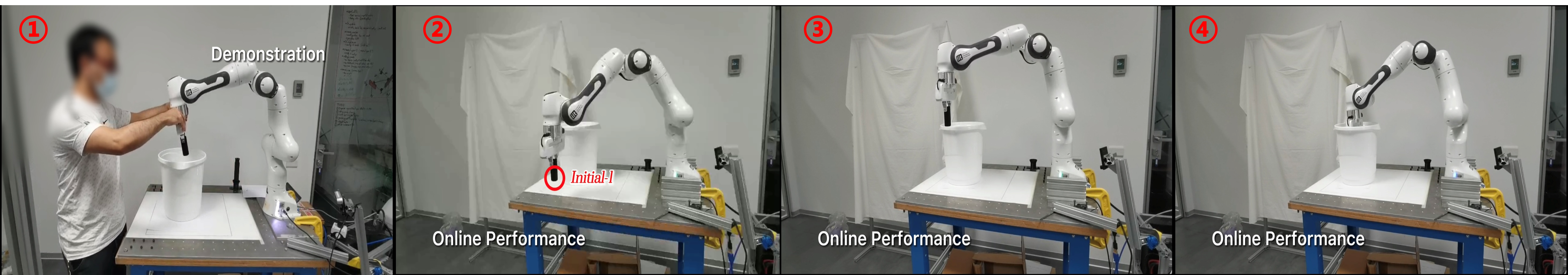
Figure 7: NES learning for the task of reaching goal locations with obstacles [78].

4.3 Dynamical system with deep RL

Deep RL methods are increasingly utilized for DSIL. Kimet al.[148] developed a hierarchical deterministic actor-critic (AC) algorithm tailored for DMP, which effectively enables robots to learn and generalize skills from human demonstrations. This algorithm excels in guiding robots through complex tasks, demonstrated by its application in a robotic arm’s pick-and-place operations.

In [149], Songet al.introduced the Deep Deterministic Policy Gradient (DDPG) algorithm, a standard RL method for the precise execution of peg-in-hole assembly tasks. This approach leverages DDPG to train a Neural Network-based Movement Primitive (NNMP), which generates continuous trajectories for force controllers, improving efficiency and stability over traditional methods.

Wanget al.[150] introduced an IL framework for complex contact-rich insertion tasks in robotics. This framework seamlessly integrates Soft Actor-Critic (SAC) and DMP to efficiently generate high-quality trajectories and force control policies. Notably, this approach demonstrates sample efficiency, enhanced safety, and superior generalization compared to conventional methods. It addresses the challenge of reducing the need for repetitive human teaching efforts by adapting learned trajectories to new tasks with similar topological characteristics, thereby alleviating the burden on human demonstrators. Changet al.[151] introduced a framework for IL to acquire both trajectory and force information from demonstrations of peg-in-hole tasks. The framework combines the use of SAC with admittance control and DMP algorithms to learn a high-level control policy that adapts impedance parameters. This approach demonstrates significant robustness even in situations with minor offsets, thereby expanding its applicability in safe and robust contact scenarios.

Sunet al.[152] introduced an actor-critic method integrated with DMP to learn controllers for nonprehensile manipulation in a hockey task. The method leverages an Optimal Replay Buffer (ORB) with ranking sampling, leading to a substantial acceleration in the convergence of the learning policy network for efficient RL. The integrated approach demonstrates the model’s effectiveness, fast learning, and generalization across different conditions.

In [153], Davchevet al.explored residual learning in IL for orientation corrections in contact-rich insertion tasks. The method integrates residual (rLfD) with RL ( Proximal Policy Optimization (PPO), SAC) to learn the residual correction policy and thus improve DMP’s generalization abilities. The approach addresses challenges posed by external factors in the environment, demonstrating increased accuracy on out-of-distribution start configurations. The study evaluates the speed of insertion and demonstrates successful policy transfer across tasks with minimal training. The residual learning technique proves effective in capturing corrections for contact-rich manipulation.

4.4 Dynamical system with other RL methods

Beyond the PI² and ES methods, there are additional approaches to RL for DSs. The Expectation Maximization (EM)-based RL method offers a probabilistic approach that facilitates flexible exploration and exploitation in robot learning. Unlike policy gradient methods, EM-RL does not require a learning rate and incorporates importance sampling to enhance the utilization of an agent’s prior experiences when estimating new exploratory parameters. The update rule is defined as:

$${\theta^{m}}\leftarrow{\theta^{m-1}}{\rm{+}}\frac{{\sum\nolimits_{i}^{\mathcal{I}}{r\left({{\theta_{i}}}\right)\left({{\theta_{i}}-{\theta^{m-1}}}\right)}}}{{\sum\nolimits_{i}^{\mathcal{I}}{r\left({{\theta_{i}}}\right)}}}$$ (48)

where ${\sum\nolimits_{i}^{\mathcal{I}}{r\left({{\theta_{i}}}\right)}}$ is the cumulative reward; $\theta^{m}$ is the policy parameter at the current iteration step $m$.

In [154, 155], Calinonet al.introduced a classical EM-based RL approach called PoWER. This method is designed to impart complex motor skills to robots, making them adept for use in human-centric environments such as homes and offices. PoWER is distinguished by its capacity to enable robots to learn DS policies, facilitating task adaptation that demands both compliance and variability, which are vital for safe and efficient human-robot interactions. Andréet al.[157] applied PoWER to enhance the walking capabilities of bipedal robots on slopes. By incorporating Central Pattern Generators (CPG) with DMP, the humanoid robot simulation was able to modify its gait for different inclines, demonstrating considerable versatility and practical application potential. Choet al.[158] expanded on PoWER by sequencing the learning and transfer of motor skills in robots according to the complexity of motion. They evaluated this complexity using temporal and spatial entropy measures across different motion trajectories. Their method streamlines the RL process, allowing robots to efficiently master and adjust motor skills from one task to another. In [159], Peterset al.developed the eNAC algorithm, a RLs approach tailored for humanoid robots’ complex motor skill acquisition. This approach integrates motor primitives with stochastic policy gradient learning, enabling the algorithm to handle the high-dimensional continuous state and action spaces of human-like limbs. In subsequent work [156], Peterset al.extended their exploration to various RLs strategies for optimizing motor primitive policy parameters. This enabled humanoid robots to master intricate tasks, exemplified by training a robotic arm to hit a baseball. Comparative analysis across different RL methods, including VPGs, PoWER, and eNAC, revealed that PoWER outperforms its counterparts in DSIL.

In [160], Koberet al.introduced the Cost-regularized Kernel Regressions method to learn the mapping from situations to meta-parameters of DMP, such as goal location, goal velocity, amplitude, duration, etc. This work innovatively applied CrKRs in an on-policy meta-parameter RLs algorithm, focusing on adapting and optimizing the meta-parameters of DMPs in tasks such as table tennis and dart throwing.

Danielet al.[161] introduced a Hierarchical Relative Entropy Policy Search (HiREPS) framework to learn a hierarchical DMPs policy acquiring versatile motor skills in robot tetherball tasks. They reformulated the task of learning a hierarchical DMPs policy as a latent variable estimation problem and employed the HiREPS framework with episodic RLs to facilitate the learning process. The experimental results indicate that HiREPS exhibits faster convergence and the ability to maintain multiple solutions, enabling the robot to wind the ball around the pole from different sides.

Figure 8: The RL performance PI-ELM for sine curve [117]. The final actual trajectories (magenta), learning curves, and the learned stiffness parameters are for different tasks, which aim to go through the via points and avoid different obstacles. The cyan arrows represent the divergent force field. The cyan dashed line is the force field boundary.

Figure 9: The RL performance PI-ELM [117]. The final actual trajectories (magenta) and learning curves are based on the demonstrations of the human handwriting motions dataset. The cyan arrows represent the constant force field.

5 Deep imitation learning

Deep learning stands out as a promising method with the potential to significantly enhance IL capabilities, as demonstrated by previous studies [166, 167]. The DSIL framework is versatile, accommodating not only low-dimensional trajectory input but also extending its application to high-dimensional image/trajectory input [168]. However, when dealing with high-dimensional inputs such as images, the challenge lies in designing an effective deep network structure and loss function that accurately represents the underlying DS.

End-to-end learning from images represents a more intuitive method for IL, particularly applicable in environments where human participation is impractical or unsafe, such as extreme or hazardous conditions. Typically, the structure of deep IL involves convolution layers for feature extraction and Multi-Layer Perceptron (MLP) to acquire the parameters of the DS. Fig. 10 illustrates an example deep IL structure.

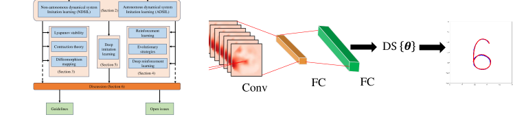
Figure 10: An example deep IL structures with high dimension image input.

In [169], Affanet al.proposed Convolutional Neural Network (CNN)-based deep-DMP to learn the mapping from the clock signal and task parameters to the forcing term of a DMP. The method employs a CNN to model the forcing terms of a Trajectory Parameterized- (TP-DMP) without requiring specialized vision systems or markers. Tested in a sweeping task with a KUKA robot, the proposed D-DMP demonstrates adaptability to new objects and robust performance against disturbances.

However, these methods do not explicitly address the challenge of defining a proper metric for evaluating networks that directly compute DMP. In [170, 171], Udeet al.introduced deep IMEDNet and Convolutional (CIMEDNet) designed to convert grayscale images into DMP. The dataset comprises MNIST and synthetic MNIST , generating image-motion pairs for training. This method effectively reconstructs handwriting movements from these image-motion pairs, showcasing the network’s ability to generalize across diverse digit variations and accurately reproduce dynamic trajectories. This suggests potential applications in human-robot interaction systems. In [172], Udeet al.further developed a spatial transformer (STIMEDNet) for image-to-motion prediction. The spatial transformer module in STIMEDNet aids in finding canonical poses for digits, significantly improving trajectory prediction accuracy under affine transformations. Consequently, STIMEDNet outperforms its predecessors, particularly excelling in predicting digit trajectories compared to the existing IMEDNet and CIMEDNet. The authors extended their approach to a humanoid robot, demonstrating its capability to recognize and reproduce handwritten digits in arbitrary poses. In [173], Udeet al.proposed a modified loss function that directly calculates the physical distance between movement trajectories, departing from the approach in [170, 171, 172] that computed the distance between DMP parameters. This new loss function can be extended to IMEDNet, CIMEDNet, STIMEDNet, Recurrent Neural Networks (RNN), etc., demonstrating superior performance compared to conventional loss functions in [170, 171, 172].

In [174], Anarossiet al.introduced a Deep Segmented Networks (DSDNet) for learning discontinuous motions through deep DMP. It presents evaluations across various tasks, including object cutting and pick-and-place, comparing DSDNet with CIMEDNet. The results demonstrate DSDNet’s superior performance in terms of generalization, task achievement, and data efficiency. DSDNet overcomes challenges faced by DSDNet, particularly in accurately predicting DMP parameters for discontinuous motions. In [175], Pahičet al.extend a previous methodology introduced in [170, 171, 172] by incorporating Arc Length- (AL-DMP). Notably advantageous over standard DMP, AL-DMP exhibit proficiency in managing paths with sharp corners and accommodating trajectories with varying speeds, making them particularly suitable for tasks such as handwriting. The paper also introduces the Variable (VIMEDNet) architecture, an extension of CIMEDNet, designed to process images of variable sizes. The efficacy of VIMEDNet in reproducing observed digits underscores its significance in handling diverse input scenarios

In [176] [177], Mavsaret al.proposed a image-to-motion recurrent NNs for the recognition of human intentions in dynamic human-robot collaboration. This work utilizes dataset consisting of video-trajectory pairs derived from assembly tasks within human-robot interaction contexts. The recurrent image-to-motion networks, trained on these datasets, employ RGB-D images to predict motion trajectories in the form of DMP parameters. Remarkably, the system not only achieves high accuracy in trajectory predictions but also enables real-time adjustments of robot trajectories based on identified human intentions. This dynamic adaptation enhances overall efficiency in shared workspaces, emphasizing the potential of RNN in optimizing human-robot collaboration scenarios. In [22], Bahlet al.developed NDPs for end-to-end sensorimotor IL. The framework incorporates the DMP structure as a differentiable layer into DNN-based policies, enabling the robot to learn directly from images and generate globally stable motions due to the convergence property inherent in DMP. The study highlights NDPs’ superior performance in IL tasks, outperforming traditional NN policies such as CIMEDNet in dynamic scenarios like digit writing. Additionally, NDPs shows enhanced efficiency and performance in RL setups compared to baseline methods such as PPO [178], demonstrating versatility across tasks with varying levels of dynamism and maintaining data efficiency. However, DNNs are inherently limited to pick-and-place-style quasi-static tasks compared to the dynamic tasks achieved by DMP-based methods. Although NDPs can improve this performance, they may face challenges in generalizing to unseen state configurations. In [179], Bahlet al.introduced Hierarchical (H-NDP) for dynamic tasks. It involves both local and global policies, with local NDPs prioritizing task success in specific regions, while the global NDPs emphasizes learning from images in a generalizable manner. This hierarchical framework, leveraging DSs, outperforms in dynamic tasks, demonstrating efficacy in capturing high-level variations and achieving better sample efficiency compared to existing methods. Additionally, H-NDPs seamlessly integrate with imitation and RL paradigms. In [180], Shawet al.introduced VideoDex, incorporating NDPs as physical priors for robot imitation from human video dataset. Utilizing 500-3000 video clips, the study highlights the importance of action priors pretrained on human internet videos for robust generalization of robot behavior. Training involves pretraining with human action priors and final policy training on teleoperated demonstrations. VideoDex consistently outperforms baselines, emphasizing the effectiveness of action priors, and the study explores the impact of physical priors and architectural choices.

The aforementioned research primarily addresses deep IL for non-autonomous DSs. Nevertheless, the same concept can be extended to autonomous neural dynamic policies, enabling end-to-end IL with high-dimensional inputs. In [181], Totsilaet al.introduced Autonomous Neural Dynamic Policies (ANDPs) for achieving stable IL in robotics. This method, building on the strengths of NDPs and the SEDS, combines NNs and autonomous DSs. ANDPs is designed to ensure asymptotically stable behaviors, making them well-suited for various IL scenarios, including those involving diverse sensor inputs like high-dimensional image observations. In [182], Auddyet al.presented a stable deep IL framework by integrating two key NN components with high-dimension trajectory input. The first NN captures the nominal dynamics model, while the second, a LF network, is built using an ICNN. This dual-network structure establishes a stable DS, facilitating effective adaptation to new tasks and the retention of knowledge from previous experiences. The incorporation of continual learning, Neural s, and hypernetworks further strengthens the model, enhancing its resilience and stability in dynamic learning environments.

6 Applications

DSIL offers a promising approach to imitate experts’ skills, simplifying the programming of robots and making it widely applicable across various scenarios. In studies such as [135], [136], and [183], rehabilitative movements were gathered from healthy individuals and trained using DSIL. These trained movements were then utilized for motion or gait generation in the rehabilitation training of exoskeleton robots. Furthermore, DSIL holds potential for applications in surgical robots, enabling them to imitate the skills of surgeons. In [138], RL combined with DSIL is utilized to learn puncturing skills under remote center motion (RCM) constraints from surgeon demonstrations. This approach allows for adaptability to different constraints without the need for re-teaching. Similarly, in [184], DSIL is integrated into a shared control framework, facilitating the transfer of skills from simulation to a da Vinci Research Kit robot for robotic surgery, such as the pick-peg task. In [185], an IL method was proposed to imitate the versatile representations of motion to continuum robots. DSIL was used to transfer motion patterns from an octopus arm to a flexible surgical robot.

Beyond medical scenarios, DSIL finds application in agricultural robots [186]. In this study, DSIL was used to encode complex activities and transfer motion skills to robotics, achieving good performance in four agricultural activities, including digging, seeding, irrigation, and harvesting. Similarly, in [187], a modified DMP-based DSIL method was proposed for ever-changing and mutable agricultural environments, enabling imitation of experts’ motion for similar agricultural activities.

For interaction or cooperative manipulation tasks where the robot involves physical contact with the environment, control of forces (torque) and positions becomes crucial. In [188], Khoramshahiet al.proposed a DSIL-based impedance control method to enable a robot to comply with human intention. This work successfully addressed transportation tasks where human and robot collaborated to carry and place a heavy object across the aisles with shelves on each side. In [39], Abu-Dakkaet al.applied a DSIL method to imitate orientation for peg-in-hole assembly tasks, considering position, orientation, and force in complex physical interaction environments.

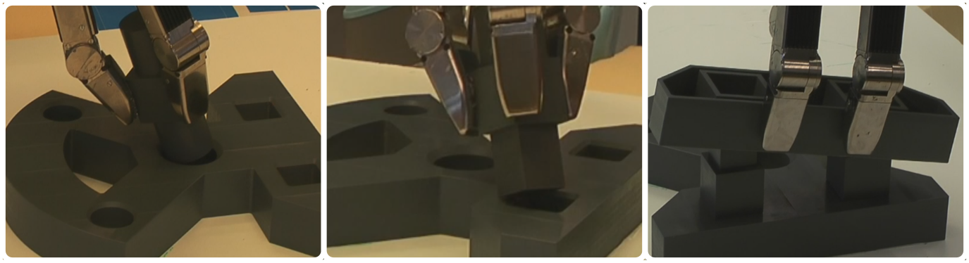
Figure 11: An example of using DSIL in Peg-in-Hole [39].

In underwater intervention tasks, DSIL plays a pivotal role in control and motion generation. In [189], Carreraet al.proposed a DSIL method to teach autonomous underwater vehicles intervention navigation towards goal positions while navigating through underwater obstacles. Similarly, in [190], Zhanget al.designed and controlled a robotic fish to achieve pose regulation in a swimming tank while considering external disturbances. To simultaneously attain the goal position and orientation, they proposed a learning framework that combined DSIL and deep reinforcement learning to train a policy from demonstrations.

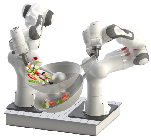
Figure 12: An example of using DSIL in cooking [191].

DSIL can also be extended to daily life tasks, such as cooking. In [191], Liuet al.modeled the skills of cooking art stir-fry and proposed a DSIL method to learn deformable object manipulation from a cook using a bimanual robot system, shown in Fig. 12.

In addition to Euclidean space, DSIL in non-Euclidean spaces such as Riemannian manifolds is also explored [114] to solve some real-world applications, e.g., bottle stacking shown in Fig. 13, that involves non-Euclidean data, e.g., orientation and impedance. Their approach discusses the utilization of mathematical techniques derived from differential geometry to ensure that learned skills adhere to the geometric constraints imposed by these complex spaces. The bottle stacking application highlights the versatility of DSIL-based trajectory generators, allowing for convergence to different goals even within complex non-Euclidean environments.

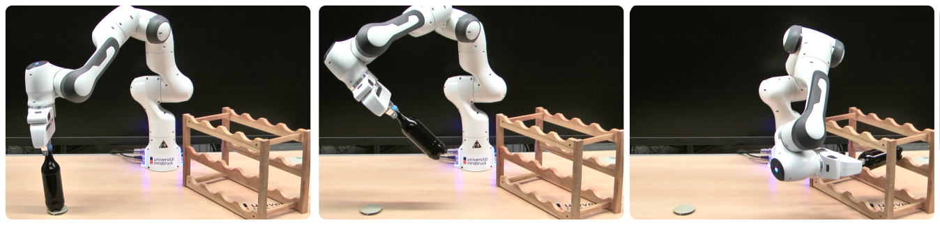
Figure 13: An example of using DSIL in Bottle Stacking [114].

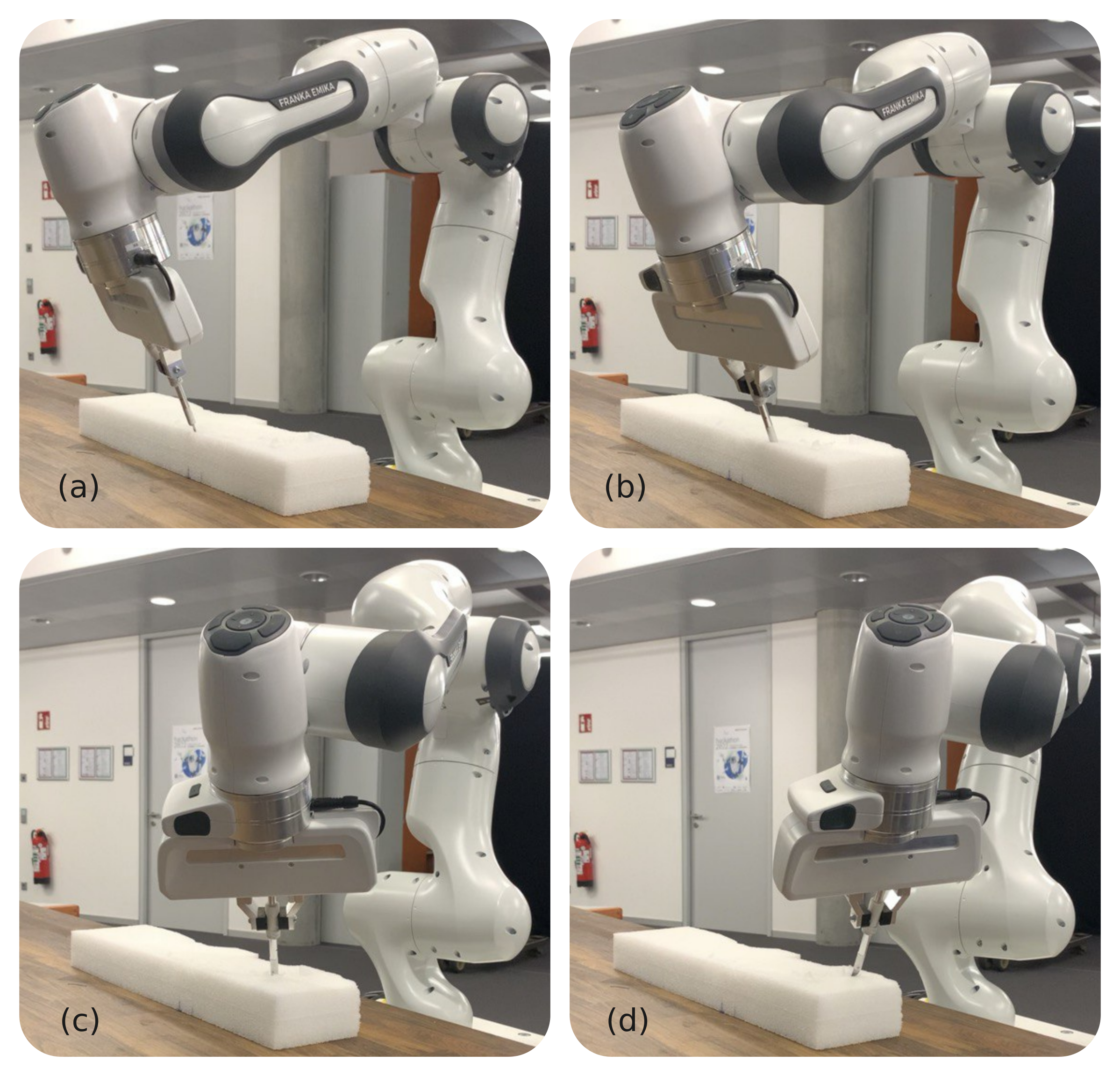
Figure 14: An illustration showcasing the application of DSIL in assisted teleoperation for cutting skills [192].

Another example of innovative use of DSIL in non-Euclidean spaces, ensuring the safe execution of learning orientation skills, represented in Lie group SO(3), within constrained regions surrounding a reference trajectory, shown in [192]. The approach involves learning a stable DS on SO(3), extracting time-varying conic constraints from expert demonstrations’ variability, and bounding the DS evolution with conic Control Barrier Function (CBF) to fulfill these constraints. This approach holds promise for applications such as tissue resection in robotic surgery, where the precise orientation of surgical instruments is crucial for performing delicate procedures accurately and safely. Figure 14 is an illustrative example of such cutting skills.

7 Discussion

The fusion of machine learning and DSs in the context of robot IL is a burgeoning topic that has captivated significant attention within the research community, setting the stage for further investigation. Despite notable achievements across diverse domains, particularly in robotics, several challenges persist, especially in complex environments. In this section, we discuss the limitations of DSIL and outline potential future research directions.

Table 11: A comparison of the main approaches for DSIL.

Approach		Advantages	Disadvantages
Existing	Stability methods	• Model-based solutions, leading to more efficient learning, faster convergence, and reduced computational requirements. • Robustness which ensures effectiveness in the presence of uncertainties or variations in the environment. • The stability contributes to overall system safety, minimizing the likelihood of unsafe actions in real-world applications. • Enhance generalization making them applicable across a diverse range of scenarios. • Facilitate the convergence and ensure that the training process is more reliable and converges to effective policies. • Often require fewer training samples, leading to more efficient and economical training processes. • Align with fundamental principles of control theory, providing a solid theoretical foundation for the design and analysis of DSIL. This integration can lead to more principled and well-understood control strategies.	• Over-reliance on simplified models which could lead to limitations in handling intricate environments. • Complex systems with nonlinear dynamics may pose challenges for stability methods, as these methods might struggle to accurately model and account for nonlinear behaviors. • Despite their robustness, stability methods may face difficulties in generalizing well to entirely unforeseen or extreme conditions that were not adequately represented in the training data. • Stability methods might encounter difficulties in effectively handling high-dimensional state or action spaces, limiting their applicability in certain complex robotic tasks. • The success of stability methods relies heavily on having an accurate understanding of the underlying system dynamics. In cases where these dynamics are not well-known, the effectiveness of stability methods may be compromised.
	Exploration learning	• Actively exploring the state-action space, making the learned policies more resilient to uncertainties and variations in the environment. • Promote better generalization, allowing the learned policies to perform well across a wider range of scenarios, including those not encountered during training. • Mitigate the risk of getting stuck in local optima by encouraging the exploration of different regions of the state-action space. • Strike a balance between exploration (trying new actions) and exploitation (leveraging known actions), optimizing the trade-off to efficiently discover and exploit rewarding policies. • Facilitate the adaptation of learned policies to changing environments by continuously exploring and updating the model based on new information.	• Active exploration methods may incur higher computational or time costs. • Improper balance between exploration and exploitation may lead to suboptimal policies or inefficient learning. • Excessive exploration can introduce noise in the learning process, leading to a less stable policy. • The effectiveness of exploration learning is closely tied to the chosen exploration strategy. • Sensitivity to hyperparameters. • Limited exploration in limited time. • They may face challenges in high-dimensional state or action spaces, where the search for informative experiences becomes more complex.
	Deep IL	• Excel at automatically learning intricate representations of the input data, enabling the model to capture complex relationships in high-dimensional state and action spaces. • They can automatically extract hierarchical features, allowing them to capture both low-level details and high-level abstractions in the dynamical system, facilitating more effective policy learning. • Enable end-to-end learning, which simplifies the modeling process and allows the model to learn directly from raw input data. • Well-suited for capturing nonlinear relationships in dynamical systems, making them effective in scenarios where the underlying dynamics are complex and nonlinear. • Continuous improvement with more data.	• Often require large amounts of labeled training data to effectively learn complex representations, and obtaining such datasets may be challenging or expensive. • Training can be computationally intensive, requiring significant computational resources, which may limit their applicability in resource-constrained environments. • Overfitting risk. • Hyperparameter sensitivity. • Adapting deep IL models to non-stationary environments, where the underlying dynamics change over time, can be challenging, potentially leading to degradation in performance.

Envisioned

• Accuracy, stability, and adaptability: DSIL is expected to demonstrate high accuracy and stability in imitation, along with the ability to adapt to new tasks without requiring re-teaching from experts. • Data-efficiency in learning: The system should exhibit efficiency in learning by effectively adapting to a wide range of scenarios with minimal demonstrations. • Safety exploration: Particularly in physical systems like robots, safety during exploration is crucial. DSIL should prioritize safety through RL or evolution strategies in real-world environments. • High-dimensional inputs: The capability to imitate from high-dimensional inputs, such as images or videos, is essential for addressing the complexity of real-world tasks in DSIL.

7.1 Guidelines

The preceding sections have provided an overview of two categories of DSIL and the varied approaches within this domain. Recognizing that each DSIL system or approach is designed to address specific conditions in applications, this section will delve into: (i) Advantages and Disadvantages: A comprehensive discussion on the merits and drawbacks of different DSIL systems and mentioned approaches provides a nuanced understanding of their strengths and limitations. (ii) Potential Challenges: Identification and exploration of potential challenges in the context of DSIL, shedding light on areas that require further attention and innovative solutions.

7.1.1 NDSIL vs DSIL

In the context of IL, a spectrum of machine learning models can represent either DS or non-autonomous DS. The distinction between NDSIL and ADSIL reveals a mutually exclusive relationship. Non-autonomous models, such as DMP [14, 15] and HSMMs [62], offer flexibility in mimicking time-varying behavior, proving beneficial for adaptation to changing conditions and providing a realistic representation of system dynamics. These models are particularly suited for systems influenced by external inputs or time-dependent factors.

Nevertheless, non-autonomous models come with drawbacks, including (i) increased complexity in learning algorithms, (ii) challenges in interpreting and analyzing models, (iii) dependency on high-quality training pairs, and (iv) heightened computational demands compared to autonomous systems.

Autonomous systems, such as SEDS [18], characterized by stable behavior, excel in learning and generalization. They can cease at any time step without altering the agent’s agent state, and their lack of external influences simplifies the prediction and understanding of the model’s behavior over time. Although autonomous systems may lack flexibility in capturing time-varying dynamics, they stand out in stability, predictability, and simplicity, making them suitable for time-independent applications.

The choice between NDSIL and ADSIL hinges on the specific requirements and characteristics of the application under consideration.

7.1.2 Choose the appropriate stability methods

Choosing the most suitable stability method depends on the specific characteristics and requirements of the DS under consideration. Each method has its unique strengths and limitations, making them more or less suitable for different application scenarios.

Lyapunov stability method is versatile and applicable to a broad spectrum of DSs, serving as a fundamental stability analysis tool. It provides a robust theoretical foundation, facilitating the development of rigorous stability proofs. Moreover, it is well-suited for global stability analysis, offering insights into the system’s behavior across the entire state space. Nevertheless, Lyapunov stability conditions can be overly conservative, imposing strict constraints that may lead to rejecting potentially stable systems, and compromising accuracy. Additionally, identifying suitable Lyapunov candidate functions can be challenging, especially for complex or nonlinear systems, thereby limiting its applicability.

CT stability method offers an effective alternative for nonlinear and time-varying systems, quantifying contraction properties and providing a metric for trajectory convergence. Moreover, it excels in robust stability analysis, demonstrating resilience to disturbances and uncertainties. Nevertheless, the computational complexity of implementing contraction metrics, particularly for high-dimensional systems, can impact real-time applications. Although it is effective for nonlinear systems, CT may not be the preferred choice for linear systems, where simpler techniques like Lyapunov stability are more straightforward.

The diffeomorphism stability method preserves topological properties, ensuring stability without sacrificing critical structural features. Moreover, it applies to chaotic systems [193], providing a method to stabilize and control chaotic behavior. Diffeomorphisms are inherently smooth transformations, ensuring smooth transitions in the state space. However, implementing diffeomorphism-based stability methods can be complex, especially for high-dimensional systems. Although diffeomorphism-based stability methods are powerful, their theoretical foundation may not be as established and general as Lyapunov stability.

Stability methods (Lyapunov, CT, and diffeomorphism) rely on accurate models of DSIL, posing challenges in deriving precise stability conditions, especially for complex models such as deep NNs.

7.1.3 Safety of policy improvement

The incorporation of exploration techniques enhances the efficiency of DSIL in exploring complex and uncharted tasks. This is particularly valuable, in scenarios, when the initial dataset lacks coverage of all possible situations. Combining DSIL with exploration strategies, such as those from RL, deep RL, or ES, enhances the robot’s ability to generalize learned policies. This adaptability is crucial for navigating diverse and dynamic environments. By incorporating exploration techniques, DSIL gains flexibility beyond the limitations of demonstrations, proving beneficial in real-world scenarios when encountering novel situations absent from the training data.

However, ensuring the safety of robotic systems is important to prevent damage. Operating within appropriate workspaces and adhering to joint physical limitations becomes challenging, especially in policy exploration scenarios using RL within DSIL. Safety requirements impose constraints on the robot’s exploration space, potentially impeding the discovery of optimal policies and leading to suboptimal outcomes.

Therefore, the policy parameters getting stuck in locally optimal solutions while considering safety constraints in safe exploration presents a significant challenge. The candidate solutions are listed as follows:

• Diverse exploration: Implement strategies that encourage RL agents to explore various actions and states to avoid getting trapped in local optima.

• Soft constraint relaxation: Temporarily relax safety constraints during training to allow for more exploration without compromising safety.

• Reward shaping: Adjust reward functions to discourage unsafe actions, guiding RL agents towards safer policies.

• Prioritized experience replay: Emphasize experiences with safety violations in the replay buffer, helping RL agents learn from past mistakes.

Among exploration methods, PI² operates as a closed-loop method, lacking explicit gradient information for guiding policy improvement. Alternately, ES methods function as open-loop ones, capable of combining with policy gradients but utilizing gradient information solely as sorting indices for the next generation. Addressing limitations inherent in each approach involves a promising solution: combining policy gradients with PI², as demonstrated by studies like [117] and [194]. This hybrid approach leverages the strengths of both methods, using gradient information within the closed-loop framework of PI² for more informed policy improvement. This integration facilitates a more robust and effective exploration strategy while maintaining a focus on safety considerations.

7.1.4 Build deep DSIL model

Harnessing the capabilities of DNNs offers a promising avenue for enabling robots to learn directly from high-dimensional data, e.g., images and videos. This approach facilitates the direct acquisition of stability skills directly from perceptual inputs. The DS model is constructed using DNNs, providing increased flexibility and trainability compared to traditional machine learning models, which is particularly valuable for when tackling complex tasks.

The primary challenge in the context of deep DSIL lies in ensuring stability. While related works, such as IMEDNet, NDPs and STIMEDNet, leverage DMP and inherit global stability, establishing stability conditions for general deep DSIL model becomes intricate due to the absence of an explicit expression. Similarly, incorporating additional constraints or employing policy exploration methods within the deep DSIL model poses challenges.

Furthermore, related works, including IMEDNet, NDPs and STIMEDNet have been trained with MNIST and synthetic MNIST image-motion pairs dataset. The challenge lies in collecting a diverse motion-image pairs dataset for various tasks.

The advantages and disadvantages of the surveyed approaches are summarized in Table 11.

7.2 Challenges and future directions

7.2.1 Dataset

In IL, the dataset plays a crucial role by providing the expert policy. It consists of pairs of observations and corresponding actions, helping the algorithm in learning to mimic expert behavior.

Imperfect or limited data: Typically, IL relies on high-quality demonstration data. However, real-world demonstrations often lack structure, containing noise and outliers. Therefore, it necessitates the development of algorithms for automatically identifying and handling unstructured data, ensuring that the learning algorithm prioritizes meaningful information. Future research avenues include exploring advanced filtering methods [195] and outlier detection algorithms [196] to enhance the model’s resilience to noisy demonstrations, thereby promoting more accurate learning.

Acquiring a substantial number of expert demonstrations is often impractical or expensive. Future research endeavors should explore strategies for efficient learning from limited demonstrations. Techniques like data augmentation [195, 197], transfer learning [198], and one-/few-shot learning [199, 200] can be investigated to optimize the utility of scarce data resources. For instance, the Data Aggregation Approach (DAgger) [201, 202] continually engages with the environment to generate new data and seeks guidance from the expert policy on the newly generated data. The algorithm iteratively enhances the dataset by integrating both cloned and expert-guided samples. Similar strategies can be employed to enhance the efficiency of sample utilization in DSIL.

High dimension data: Section 5 partially addresses aspects of handling high-dimensional data in DSIL through models like IMEDNet, NDPs, STIMEDNet, and VIMEDNet. However, the reliance on motion-image pairs data presents a challenge for effectively utilizing pure image or video data in DSIL.

The primary challenge lies in developing robust feature extraction methods for high-dimensional data. The objective is to derive temporal logic trajectories through IL from images, a task that differs from conventional image processing tasks in deep learning. Secondly, as DSIL is a set of differential equations, the main challenge is to represent the DSIL model as a deep DS. This representation should handle the intricacies of high-dimensional input-output mappings, addressing stability, robustness, safety constraints, and more. Additionally, real-time performance becomes a challenge due to the potential increase in computational demands with high-dimensional input.

Future directions may concentrate on constructing a deep DSIL model adept at extracting robust features from images to facilitate motion imitation. Additionally, emphasis can be placed on integrating considerations of stability, robustness, and safety constraints into the model for comprehensive performance. These advancements aim to enhance the adaptability and efficiency of DSIL models when dealing with high-dimensional data.

Geometry-constrained data: Traditional DSIL encounters challenges in directly encoding skills with geometry constraints, particularly concerning orientation data [162]. Integrating unit quaternions, for instance, may not maintain quaternion norm unity, requiring additional constraints during integration. While DSIL has partially addressed geometry constraints with specific data types, such as orientation profiles [203], stiffness/damping [163], and manipulability profiles (manifold of SPD data) [45], extending similar approaches to other Riemannian manifolds like the Grassmannian or Hyperbolic manifolds remains non-trivial and has not been fully addressed [15].

Future work can extend the DSIL method to other Riemannian manifolds and represent the geometry constraints with specific data types. This extension aims to enhance the applicability and versatility of DSIL in handling a broader range of geometry-constrained data, providing more comprehensive solutions for encoding skills in various robotic applications.

7.2.2 Skills generalization

Accuracy and stability: Achieving robustness to task variability while maintaining accuracy presents a pivotal challenge in skills generalization. The conflict between accuracy and stability arises in modeling non-monotonic dynamics, particularly scenarios where the system temporarily moves away from the attractor [106]. Despite existing efforts to partially resolve the conflict between stability and accuracy with less conservative stability conditions, such as CLF-DM [19], and NS-QLF [88, 93] (as discussed in Section 3), there remains a gap in simultaneously improving robustness and accuracy. The current state of research highlights the need for advancements to harmoniously blend stability, accuracy, and robustness in DSIL models.

The concentration on single-attractor DS, unless stability constraints are integrated, demands prior knowledge of the attractor’s location. This assumption significantly limits the applicability of stability methods to learning uni-modal dynamics. The incorporation of multiple dynamics into a single control law based on DS adds complexity to effectively model a broader range of dynamical behaviors [106].

Future research avenues should be directed towards enhancing DSIL model performance to achieve a harmonious balance between stability, accuracy, and robustness. Advancements in this direction will contribute to the broader adoption of DSIL models in real-world applications with diverse and dynamic task environments.

Unseen configurations: A significant challenge in DSIL arises from the limitations of covering all situations within the demonstrations. IL models often encounter difficulties when confronted with scenarios featuring configurations not present in the training demonstrations. To overcome this challenge, research should focus on enabling models to extrapolate knowledge from existing demonstrations, allowing them to handle novel and unseen situations. This entails exploring techniques that capture underlying dynamics capable of generalizing well across diverse environments, and recognizing the inadequacy of imitating a static set of demonstrations for dynamic and evolving environments.

Addressing the domain adaptation problem of unseen configurations, transfer learning is a candidate solution [204]. This method facilitates the transfer of acquired skills across diverse domains. Domain adaptation is particularly evident in scenarios involving IL with policy exploration using RL, such as simulation-to-real, simulation-to-simulation, and real-to-real transitions [205]. To effectively tackle this challenge, future investigations should concentrate on exploring domain adaptation methods [206]. These endeavors aim to enhance the transferability of acquired skills, ensuring their applicability and effectiveness across varied and dynamic environments.

Another solution involves exploring continual learning methods [207] tailored for handling unseen configurations. This approach allows the model to adapt incrementally to new situations over time, accumulating knowledge from ongoing interactions. Potential research directions include advancements in transfer learning, where efforts could be directed toward developing transferable knowledge representations that empower the model to adapt efficiently to new and unseen situations.

Advanced learning methods: Although Bahlet al.proposed the structure of a deep DSIL–NDPs in [22], a persistent challenge in the continuous evolution of deep IL is the limited capacity of existing models to adequately represent the diversity of movements. Consequently, the construction of a larger DSIL model remains an ongoing challenge. The progress in Large Language Model (LLM) offers a promising solution for DSIL [208]. LLMs possess the capability to directly learn from diverse data modalities, including language, images, and trajectories, leading to improved skill generalization. This opens up new possibilities for enhancing the versatility and adaptability of robot IL systems. By harnessing the expressive power of LLMs, robots can better comprehend the contextual nuances of instructions, interpret visual cues from images, and assimilate the temporal dynamics of trajectories. This holistic learning approach enables the robot to generalize acquired skills across a broader spectrum of tasks and scenarios.

In addition to LLMs, drawing inspiration from the work of Neural ODE by Chenet al.[209], which utilizes ODEs to model the dynamics of the network’s hidden states in DNNs. Instead of using discrete layers to model transformations, Neural ODEs use continuous transformations defined by differential equations. Since DSIL is a set of ODEs, future research could explore integrating Neural ODEs into DSIL [210].

Advanced control methods: Presently, most fusion of DSIL with control theory are offline methods, e.g., stability method LF. Despite the existence of online APF-based obstacle avoidance methods, as discussed in Section 2.1, such as point-static [47] and volume-dynamic [50], the challenge lies in effectively applying control methods online to enhance generalization, especially concerning stability and safety. As reported by Nawazet al.[210], a nominal DSIL was trained offline, selecting a target point at each time step using Neural ODEs. Subsequently, Control Lyapunov Function (CLF) and CBF are employed to ensure stability and safety for online motion correction. However, a limitation arises from the potential risk of converging to a local minimum due to conflicting safety and task-completion constraints. Future research directions may explore advanced online control methods to correct motion in real-time, aiming to achieve globally optimal policies for skills generalization.

Passivity-based control approach can also be used to improve the stability of first-order DSIL. In their works [163] and [211], Leeet al.introduced a passivity-based control approach aimed at creating a Variable Stiffness Dynamical System (VSDS) through the regulation of desired motion within the original dynamical system. This VSDS is distinguished by its safety, compliant interaction behavior, and ability to converge to a reference motion. Additionally, as the DSIL represents a classical dynamical system, alternative control methods such as sliding mode control [212] and adaptive control methods [213] may offer viable solutions. Future research directions may explore different control methods to improve the stability of DSIL.

8 Conclusion

In this paper, we conduct a comprehensive survey on DSIL, a theory fusion approach that combines machine learning with DSs. Our primary objective is to categorize and review the extensive literature on DSIL, employing a systematic review approach and automated searches for relevant papers. We first discuss two types of DSIL: NDSIL. We then propose a taxonomy that includes three main stability methods: Lyapunov stability, contraction theory, and diffeomorphism mapping. Our survey includes a thorough examination and comparison of policy exploration models in DSIL, encompassing traditional RL, evolution strategies methods, deep RL, and establishing a connection from PI² to ES on DSIL. Furthermore, we delve into the realm of deep IL models within DSIL. Finally, we highlight several open problems and challenges within DSIL, identifying avenues for future research.

References

- [1] Debasmita Mukherjee, Kashish Gupta, Li Hsin Chang, and Homayoun Najjaran. A survey of robot learning strategies for human-robot collaboration in industrial settings. Robotics and Computer-Integrated Manufacturing, 73:102231, 2022.
- [2] Matt Deitke, Dhruv Batra, Yonatan Bisk, Tommaso Campari, Angel X Chang, Devendra Singh Chaplot, Changan Chen, Claudia Pérez D’Arpino, Kiana Ehsani, Ali Farhadi, et al. Retrospectives on the embodied ai workshop. arXiv preprint arXiv:2210.06849, 2022.
- [3] Mehrdad Tavassoli, Sunny Katyara, Maria Pozzi, Nikhil Deshpande, Darwin G Caldwell, and Domenico Prattichizzo. Learning skills from demonstrations: A trend from motion primitives to experience abstraction. IEEE Transactions on Cognitive and Developmental Systems, 2023.
- [4] Stefan Schaal. Learning from demonstration. Advances in neural information processing systems, 9, 1996.
- [5] Petar Kormushev, Sylvain Calinon, and Darwin G Caldwell. Imitation learning of positional and force skills demonstrated via kinesthetic teaching and haptic input. Advanced Robotics, 25(5):581–603, 2011.
- [6] Pieter Abbeel, Adam Coates, and Andrew Y Ng. Autonomous helicopter aerobatics through apprenticeship learning. The International Journal of Robotics Research, 29(13):1608–1639, 2010.
- [7] YuXuan Liu, Abhishek Gupta, Pieter Abbeel, and Sergey Levine. Imitation from observation: Learning to imitate behaviors from raw video via context translation. In 2018 IEEE International Conference on Robotics and Automation (ICRA), pages 1118–1125. IEEE, 2018.
- [8] Ioannis Havoutis and Sylvain Calinon. Learning from demonstration for semi-autonomous teleoperation. Autonomous Robots, 43:713–726, 2019.
- [9] Joseph DelPreto, Jeffrey I Lipton, Lindsay Sanneman, Aidan J Fay, Christopher Fourie, Changhyun Choi, and Daniela Rus. Helping robots learn: a human-robot master-apprentice model using demonstrations via virtual reality teleoperation. In 2020 IEEE International Conference on Robotics and Automation (ICRA), pages 10226–10233. IEEE, 2020.
- [10] Yonadav Shavit, Nadia Figueroa, Seyed Sina Mirrazavi Salehian, and Aude Billard. Learning augmented joint-space task-oriented dynamical systems: a linear parameter varying and synergetic control approach. IEEE Robotics and Automation Letters, 3(3):2718–2725, 2018.
- [11] Zhuangdi Zhu, Kaixiang Lin, Bo Dai, and Jiayu Zhou. Off-policy imitation learning from observations. Advances in Neural Information Processing Systems, 33:12402–12413, 2020.
- [12] Tianhao Zhang, Zoe McCarthy, Owen Jow, Dennis Lee, Xi Chen, Ken Goldberg, and Pieter Abbeel. Deep imitation learning for complex manipulation tasks from virtual reality teleoperation. In 2018 IEEE International Conference on Robotics and Automation (ICRA), pages 5628–5635. IEEE, 2018.
- [13] Affan Pervez, Arslan Ali, Jee-Hwan Ryu, and Dongheui Lee. Novel learning from demonstration approach for repetitive teleoperation tasks. In 2017 IEEE World Haptics Conference (WHC), pages 60–65. IEEE, 2017.
- [14] Auke Jan Ijspeert, Jun Nakanishi, Heiko Hoffmann, Peter Pastor, and Stefan Schaal. Dynamical movement primitives: learning attractor models for motor behaviors. Neural computation, 25(2):328–373, 2013.
- [15] Matteo Saveriano, Fares J Abu-Dakka, Aljaž Kramberger, and Luka Peternel. Dynamic movement primitives in robotics: A tutorial survey. The International Journal of Robotics Research, 42(13):1133–1184, 2023.
- [16] Sylvain Calinon, Zhibin Li, Tohid Alizadeh, Nikos G Tsagarakis, and Darwin G Caldwell. Statistical dynamical systems for skills acquisition in humanoids. In 2012 12th IEEE-RAS International Conference on Humanoid Robots (Humanoids 2012), pages 323–329. IEEE, 2012.
- [17] Hang Su, Yingbai Hu, Hamid Reza Karimi, Alois Knoll, Giancarlo Ferrigno, and Elena De Momi. Improved recurrent neural network-based manipulator control with remote center of motion constraints: Experimental results. Neural Networks, 131:291–299, 2020.
- [18] S Mohammad Khansari-Zadeh and Aude Billard. Learning stable nonlinear dynamical systems with gaussian mixture models. IEEE Transactions on Robotics, 27(5):943–957, 2011.
- [19] S Mohammad Khansari-Zadeh and Aude Billard. Learning control lyapunov function to ensure stability of dynamical system-based robot reaching motions. Robotics and Autonomous Systems, 62(6):752–765, 2014.
- [20] Tamim Asfour, Pedram Azad, Florian Gyarfas, and Rüdiger Dillmann. Imitation learning of dual-arm manipulation tasks in humanoid robots. International journal of humanoid robotics, 5(02):183–202, 2008.
- [21] Dennis Herzog, Aleš Ude, and Volker Krüger. Motion imitation and recognition using parametric hidden markov models. In Humanoids 2008-8th IEEE-RAS International Conference on Humanoid Robots, pages 339–346. IEEE, 2008.
- [22] Shikhar Bahl, Mustafa Mukadam, Abhinav Gupta, and Deepak Pathak. Neural dynamic policies for end-to-end sensorimotor learning. Advances in Neural Information Processing Systems, 33:5058–5069, 2020.
- [23] Michail Theofanidis, Asil Bozcuoglu, and Maria Kyrarini. Learning visuomotor policies with deep movement primitives. In The 14th PErvasive Technologies Related to Assistive Environments Conference, pages 140–146, 2021.
- [24] Stefan Schaal. Is imitation learning the route to humanoid robots? Trends in cognitive sciences, 3(6):233–242, 1999.
- [25] Aude Billard, Sylvain Calinon, Ruediger Dillmann, and Stefan Schaal. Survey: Robot programming by demonstration. Technical report, Springrer, 2008.
- [26] Brenna D Argall, Sonia Chernova, Manuela Veloso, and Brett Browning. A survey of robot learning from demonstration. Robotics and autonomous systems, 57(5):469–483, 2009.
- [27] Aude Billard and Daniel Grollman. Robot learning by demonstration. Scholarpedia, 8(12):3824, 2013.
- [28] Zuyuan Zhu and Huosheng Hu. Robot learning from demonstration in robotic assembly: A survey. Robotics, 7(2):17, 2018.
- [29] Sylvain Calinon. Learning from demonstration (programming by demonstration). Encyclopedia of robotics, pages 1–8, 2018.
- [30] ZongWu Xie, Qi Zhang, ZaiNan Jiang, and Hong Liu. Robot learning from demonstration for path planning: A review. Science China Technological Sciences, 63(8):1325–1334, 2020.
- [31] Harish Ravichandar, Athanasios S Polydoros, Sonia Chernova, and Aude Billard. Recent advances in robot learning from demonstration. Annual review of control, robotics, and autonomous systems, 3:297–330, 2020.
- [32] Weiyong Si, Ning Wang, and Chenguang Yang. A review on manipulation skill acquisition through teleoperation-based learning from demonstration. Cognitive Computation and Systems, 3(1):1–16, 2021.
- [33] Khansari Zadeh and Seyed Mohammad. A dynamical system-based approach to modeling stable robot control policies via imitation learning. Technical report, Epfl, 2012.
- [34] Anatole Katok, AB Katok, and Boris Hasselblatt. Introduction to the modern theory of dynamical systems. Number 54. Cambridge university press, 1995.
- [35] Michael Brin and Garrett Stuck. Introduction to dynamical systems. Cambridge university press, 2002.
- [36] Auke Jan Ijspeert, Jun Nakanishi, and Stefan Schaal. Movement imitation with nonlinear dynamical systems in humanoid robots. In 2002 International Conference on Robotics and Automation (ICRA), volume 2, pages 1398–1403. IEEE, 2002.
- [37] Alexandros Paraschos, Christian Daniel, Jan Peters, and Gerhard Neumann. Using probabilistic movement primitives in robotics. Autonomous Robots, 42:529–551, 2018.
- [38] Martijn JA Zeestraten, Sylvain Calinon, and Darwin G Caldwell. Variable duration movement encoding with minimal intervention control. In 2016 IEEE International Conference on Robotics and Automation (ICRA), pages 497–503. IEEE, 2016.
- [39] Fares J. Abu-Dakka, Bojan Nemec, Jimmy A. Jørgensen, Thiusius R. Savarimuthu, Norbert Krüger, and Aleš Ude. Adaptation of manipulation skills in physical contact with the environment to reference force profiles. Autonomous Robots, 39(2):199–217, 2015.
- [40] Matteo Saveriano, Felix Franzel, and Dongheui Lee. Merging position and orientation motion primitives. In 2019 International Conference on Robotics and Automation (ICRA), pages 7041–7047. IEEE, 2019.
- [41] Ibrahim A Seleem, Samy FM Assal, Hiroyuki Ishii, and Haitham El-Hussieny. Guided pose planning and tracking for multi-section continuum robots considering robot dynamics. IEEE Access, 7:166690–166703, 2019.
- [42] Ibrahim A Seleem, Haitham El-Hussieny, Samy FM Assal, and Hiroyuki Ishii. Development and stability analysis of an imitation learning-based pose planning approach for multi-section continuum robot. IEEE Access, 8:99366–99379, 2020.
- [43] Antonis Sidiropoulos, Yiannis Karayiannidis, and Zoe Doulgeri. Human-robot collaborative object transfer using human motion prediction based on cartesian pose dynamic movement primitives. In 2021 IEEE International Conference on Robotics and Automation (ICRA), pages 3758–3764. IEEE, 2021.
- [44] Leonidas Koutras and Zoe Doulgeri. A correct formulation for the orientation dynamic movement primitives for robot control in the cartesian space. In Conference on robot learning, pages 293–302. PMLR, 2020.
- [45] Fares J. Abu-Dakka and Ville Kyrki. Geometry-aware dynamic movement primitives. In IEEE International Conference on Robotics and Automation, pages 4421–4426, Paris, France, 2020.
- [46] Heiko Hoffmann, Peter Pastor, Dae-Hyung Park, and Stefan Schaal. Biologically-inspired dynamical systems for movement generation: Automatic real-time goal adaptation and obstacle avoidance. In 2009 IEEE international conference on robotics and automation, pages 2587–2592. IEEE, 2009.
- [47] Charles W Warren. Global path planning using artificial potential fields. In 1989 IEEE International Conference on Robotics and Automation, pages 316–317. IEEE Computer Society, 1989.
- [48] Michele Ginesi, Daniele Meli, Andrea Calanca, Diego Dall’Alba, Nicola Sansonetto, and Paolo Fiorini. Dynamic movement primitives: Volumetric obstacle avoidance. In 2019 19th international conference on advanced robotics (ICAR), pages 234–239. IEEE, 2019.
- [49] Dae-Hyung Park, Heiko Hoffmann, Peter Pastor, and Stefan Schaal. Movement reproduction and obstacle avoidance with dynamic movement primitives and potential fields. In Humanoids 2008-8th IEEE-RAS International Conference on Humanoid Robots, pages 91–98. IEEE, 2008.
- [50] Michele Ginesi, Daniele Meli, Andrea Roberti, Nicola Sansonetto, and Paolo Fiorini. Dynamic movement primitives: Volumetric obstacle avoidance using dynamic potential functions. Journal of Intelligent & Robotic Systems, 101:1–20, 2021.
- [51] Yingbai Hu, Guang Chen, Longbin Zhang, Hang Su, Mengyao Li, Yunus Schmirander, Hu Cao, and Alois Knoll. Fuzzy adaptive control-based real-time obstacle avoidance under uncertain perturbations. In 2020 5th International Conference on Advanced Robotics and Mechatronics (ICARM), pages 50–55. IEEE, 2020.
- [52] Radhe Shyam Sharma, Santosh Shukla, Hamad Karki, Amit Shukla, Laxmidhar Behera, and KS Venkatesh. Dmp based trajectory tracking for a nonholonomic mobile robot with automatic goal adaptation and obstacle avoidance. In 2019 International Conference on Robotics and Automation (ICRA), pages 8613–8619. IEEE, 2019.
- [53] Èric Pairet, Paola Ardón, Michael Mistry, and Yvan Petillot. Learning generalizable coupling terms for obstacle avoidance via low-dimensional geometric descriptors. IEEE Robotics and Automation Letters, 4(4):3979–3986, 2019.
- [54] Robert Krug and Dimitar Dimitrovz. Representing movement primitives as implicit dynamical systems learned from multiple demonstrations. In 2013 16th International Conference on Advanced Robotics (ICAR), pages 1–8. IEEE, 2013.
- [55] Robert Krug and Dimitar Dimitrov. Model predictive motion control based on generalized dynamical movement primitives. Journal of Intelligent & Robotic Systems, 77:17–35, 2015.
- [56] Yingbai Hu, Mingyang Cui, Jianghua Duan, Wenjun Liu, Dianye Huang, Alois Knoll, and Guang Chen. Model predictive optimization for imitation learning from demonstrations. Robotics and Autonomous Systems, 163:104381, 2023.
- [57] Sylvain Calinon, Florent Guenter, and Aude Billard. On learning, representing, and generalizing a task in a humanoid robot. IEEE Transactions on Systems, Man, and Cybernetics, Part B (Cybernetics), 37(2):286–298, 2007.
- [58] Sylvain Calinon, Irene Sardellitti, and Darwin G Caldwell. Learning-based control strategy for safe human-robot interaction exploiting task and robot redundancies. In 2010 IEEE/RSJ International Conference on Intelligent Robots and Systems, pages 249–254. IEEE, 2010.
- [59] Sylvain Calinon, Florent D’halluin, Eric L Sauser, Darwin G Caldwell, and Aude G Billard. Learning and reproduction of gestures by imitation. IEEE Robotics & Automation Magazine, 17(2):44–54, 2010.
- [60] Sylvain Calinon, Tohid Alizadeh, and Darwin G Caldwell. On improving the extrapolation capability of task-parameterized movement models. In 2013 IEEE/RSJ international conference on intelligent robots and systems, pages 610–616. IEEE, 2013.
- [61] Sylvain Calinon, Florent D’halluin, Darwin G Caldwell, and Aude G Billard. Handling of multiple constraints and motion alternatives in a robot programming by demonstration framework. In 2009 9th IEEE-RAS International Conference on Humanoid Robots, pages 582–588. IEEE, 2009.
- [62] Sylvain Calinon, Antonio Pistillo, and Darwin G Caldwell. Encoding the time and space constraints of a task in explicit-duration hidden markov model. In 2011 IEEE/RSJ International Conference on Intelligent Robots and Systems, pages 3413–3418. IEEE, 2011.
- [63] Elena Gribovskaya and Aude Billard. Combining dynamical systems control and programmingby demonstration for teaching discrete bimanual coordination tasks to a humanoid robot. In Proceedings of the 3rd ACM/IEEE international conference on Human robot interaction, pages 33–40, 2008.
- [64] Denis Forte, Andrej Gams, Jun Morimoto, and Aleš Ude. On-line motion synthesis and adaptation using a trajectory database. Robotics and Autonomous Systems, 60(10):1327–1339, 2012.
- [65] Ge Li, Zeqi Jin, Michael Volpp, Fabian Otto, Rudolf Lioutikov, and Gerhard Neumann. Prodmp: A unified perspective on dynamic and probabilistic movement primitives. IEEE Robotics and Automation Letters, 8(4):2325–2332, 2023.
- [66] Seyed Mohammad Khansari-Zadeh and Aude Billard. A dynamical system approach to realtime obstacle avoidance. Autonomous Robots, 32:433–454, 2012.
- [67] Andre Lemme, Klaus Neumann, René Felix Reinhart, and Jochen J Steil. Neural learning of vector fields for encoding stable dynamical systems. Neurocomputing, 141:3–14, 2014.
- [68] Jianghua Duan, Yongsheng Ou, Jianbing Hu, Zhiyang Wang, Shaokun Jin, and Chao Xu. Fast and stable learning of dynamical systems based on extreme learning machine. IEEE Transactions on Systems, Man, and Cybernetics: Systems, 49(6):1175–1185, 2017.
- [69] Klaus Neumann and Jochen J Steil. Learning robot motions with stable dynamical systems under diffeomorphic transformations. Robotics and Autonomous Systems, 70:1–15, 2015.
- [70] Zhehao Jin, Weiyong Si, Andong Liu, Wen-An Zhang, Li Yu, and Chenguang Yang. Learning a flexible neural energy function with a unique minimum for globally stable and accurate demonstration learning. IEEE Transactions on Robotics, 2023.
- [71] Nadia Barbara Figueroa Fernandez and Aude Billard. A physically-consistent bayesian non-parametric mixture model for dynamical system learning. Proceedings of Machine Learning Research, 2018.
- [72] Shaokun Jin, Zhiyang Wang, Yongsheng Ou, and Wei Feng. Learning accurate and stable dynamical system under manifold immersion and submersion. IEEE Transactions on Neural Networks and Learning Systems, 30(12):3598–3610, 2019.
- [73] Mahdi Khoramshahi, Antoine Laurens, Thomas Triquet, and Aude Billard. From human physical interaction to online motion adaptation using parameterized dynamical systems. In 2018 IEEE/RSJ International Conference on Intelligent Robots and Systems (IROS), pages 1361–1366. IEEE, 2018.
- [74] Caroline Blocher, Matteo Saveriano, and Dongheui Lee. Learning stable dynamical systems using contraction theory. In 2017 14th International Conference on Ubiquitous Robots and Ambient Intelligence (URAI), pages 124–129. IEEE, 2017.
- [75] Matteo Saveriano. An energy-based approach to ensure the stability of learned dynamical systems. In 2020 IEEE International Conference on Robotics and Automation (ICRA), pages 4407–4413. IEEE, 2020.
- [76] Ajay Kumar Tanwani and Sylvain Calinon. Learning robot manipulation tasks with task-parameterized semitied hidden semi-markov model. IEEE Robotics and Automation Letters, 1(1):235–242, 2016.
- [77] Hassan K Khalil. Lyapunov stability. Control systems, robotics and automation, 12:115, 2009.
- [78] Yingbai Hu, Guang Chen, Zhijun Li, and Alois Knoll. Robot policy improvement with natural evolution strategies for stable nonlinear dynamical system. IEEE Transactions on Cybernetics, 2022.
- [79] S Mohammad Khansari-Zadeh and Aude Billard. Imitation learning of globally stable non-linear point-to-point robot motions using nonlinear programming. In 2010 IEEE/RSJ International Conference on Intelligent Robots and Systems, pages 2676–2683. IEEE, 2010.
- [80] Sheng Xu, Jia Liu, Chenguang Yang, Xinyu Wu, and Tiantian Xu. A learning-based stable servo control strategy using broad learning system applied for microrobotic control. IEEE Transactions on Cybernetics, 52(12):13727–13737, 2021.
- [81] Yanwei Wang, Nadia Figueroa, Shen Li, Ankit Shah, and Julie Shah. Temporal logic imitation: Learning plan-satisficing motion policies from demonstrations. arXiv preprint arXiv:2206.04632, 2022.
- [82] Patrick Göttsch, Robin Olschewski, and Herbert Werner. A segmentation scheme for clf dynamic movement control applied to robotic handwriting. IFAC-PapersOnLine, 50(1):11459–11464, 2017.
- [83] Antonio Paolillo and Matteo Saveriano. Learning stable dynamical systems for visual servoing. In 2022 International Conference on Robotics and Automation (ICRA), pages 8636–8642. IEEE, 2022.
- [84] Klaus Neumann, Andre Lemme, and Jochen J Steil. Neural learning of stable dynamical systems based on data-driven lyapunov candidates. In 2013 IEEE/RSJ International Conference on Intelligent Robots and Systems, pages 1216–1222. IEEE, 2013.
- [85] Alexandre Coulombe and Hsiu-Chin Lin. Generating stable and collision-free policies through lyapunov function learning. In 2023 IEEE International Conference on Robotics and Automation (ICRA), pages 3037–3043. IEEE, 2023.
- [86] Jonas Umlauft, Armin Lederer, and Sandra Hirche. Learning stable gaussian process state space models. In 2017 American Control Conference (ACC), pages 1499–1504. IEEE, 2017.
- [87] Lukas Pöhler, Jonas Umlauft, and Sandra Hirche. Uncertainty-based human motion tracking with stable gaussian process state space models. IFAC-PapersOnLine, 51(34):8–14, 2019.
- [88] Zhehao Jin, Dongdong Qin, Andong Liu, Wen-An Zhang, and Li Yu. Learning neural-shaped quadratic lyapunov function for stable, accurate and generalizable human–robot skills transfer. Robotics and Computer-Integrated Manufacturing, 82:102526, 2023.
- [89] J Zico Kolter and Gaurav Manek. Learning stable deep dynamics models. Advances in neural information processing systems, 32, 2019.
- [90] Amin Abyaneh and Hsiu-Chin Lin. Learning lyapunov-stable polynomial dynamical systems through imitation. In 7th Annual Conference on Robot Learning, 2023.
- [91] Paul Gesel and Momotaz Begum. Learning stable dynamics via iterative quadratic programming. In 2023 IEEE International Conference on Robotics and Automation (ICRA), pages 2958–2964. IEEE, 2023.
- [92] Hiroyasu Tsukamoto, Soon-Jo Chung, and Jean-Jaques E Slotine. Contraction theory for nonlinear stability analysis and learning-based control: A tutorial overview. Annual Reviews in Control, 52:135–169, 2021.
- [93] Vikas Sindhwani, Stephen Tu, and Mohi Khansari. Learning contracting vector fields for stable imitation learning. arXiv preprint arXiv:1804.04878, 2018.
- [94] Bachir El Khadir, Jake Varley, and Vikas Sindhwani. Teleoperator imitation with continuous-time safety. arXiv preprint arXiv:1905.09499, 2019.
- [95] Lukas Huber, Aude Billard, and Jean-Jacques Slotine. Avoidance of convex and concave obstacles with convergence ensured through contraction. IEEE Robotics and Automation Letters, 4(2):1462–1469, 2019.
- [96] Harish Chaandar Ravichandar, Iman Salehi, and Ashwin P Dani. Learning partially contracting dynamical systems from demonstrations. In CoRL, pages 369–378, 2017.
- [97] Harish Ravichandar. Methods for imitation learning and human intention inference: Towards seamless human-robot collaboration. 2018.
- [98] Harish Chaandar Ravichandar and Ashwin Dani. Learning position and orientation dynamics from demonstrations via contraction analysis. Autonomous Robots, 43(4):897–912, 2019.
- [99] Sumeet Singh, Spencer M Richards, Vikas Sindhwani, Jean-Jacques E Slotine, and Marco Pavone. Learning stabilizable nonlinear dynamics with contraction-based regularization. The International Journal of Robotics Research, 40(10-11):1123–1150, 2021.
- [100] Hiroyasu Tsukamoto and Soon-Jo Chung. Imitation learning for robust and safe online motion planning: A contraction theory approach. Submitted to IEEE Robot. Automat. Lett, 2021.
- [101] John Franks. Necessary conditions for stability of diffeomorphisms. Transactions of the American Mathematical Society, 158(2):301–308, 1971.
- [102] Leonid Polterovich. The geometry of the group of symplectic diffeomorphism. Birkhäuser, 2012.
- [103] Muhammad Asif Rana, Anqi Li, Dieter Fox, Byron Boots, Fabio Ramos, and Nathan Ratliff. Euclideanizing flows: Diffeomorphic reduction for learning stable dynamical systems. In Learning for Dynamics and Control, pages 630–639. PMLR, 2020.
- [104] Nicolas Perrin and Philipp Schlehuber-Caissier. Fast diffeomorphic matching to learn globally asymptotically stable nonlinear dynamical systems. Systems & Control Letters, 96:51–59, 2016.
- [105] Julen Urain, Michele Ginesi, Davide Tateo, and Jan Peters. Imitationflow: Learning deep stable stochastic dynamic systems by normalizing flows. In 2020 IEEE/RSJ International Conference on Intelligent Robots and Systems (IROS), pages 5231–5237. IEEE, 2020.
- [106] Bernardo Fichera and Aude Billard. Linearization and identification of multiple-attractor dynamical systems through laplacian eigenmaps. The Journal of Machine Learning Research, 23(1):13290–13324, 2022.
- [107] Petar Bevanda, Max Beier, Sebastian Kerz, Armin Lederer, Stefan Sosnowski, and Sandra Hirche. Diffeomorphically learning stable koopman operators. IEEE Control Systems Letters, 6:3427–3432, 2022.
- [108] Rodrigo Pérez-Dattari and Jens Kober. Stable motion primitives via imitation and contrastive learning. IEEE Transactions on Robotics, 2023. doi=10.1109/TRO.2023.3289597.
- [109] Rodrigo Pérez-Dattari, Cosimo Della Santina, and Jens Kober. Deep metric imitation learning for stable motion primitives. arXiv preprint arXiv:2310.12831, 2023.
- [110] Weiming Zhi, Tin Lai, Lionel Ott, and Fabio Ramos. Diffeomorphic transforms for generalised imitation learning. In L4DC, pages 508–519, 2022.
- [111] Julen Urain, Davide Tateo, and Jan Peters. Learning stable vector fields on lie groups. IEEE Robotics and Automation Letters, 7(4):12569–12576, 2022.
- [112] Jiechao Zhang, Hadi Beik Mohammadi, and Leonel Rozo. Learning riemannian stable dynamical systems via diffeomorphisms. In 6th Annual Conference on Robot Learning, 2022.
- [113] Weitao Wang, Matteo Saveriano, and Fares J Abu-Dakka. Learning deep robotic skills on riemannian manifolds. IEEE Access, 10:114143–114152, 2022.
- [114] Matteo Saveriano, Fares J Abu-Dakka, and Ville Kyrki. Learning stable robotic skills on riemannian manifolds. Robotics and Autonomous Systems, 169:104510, 2023.
- [115] Petar Kormushev, Sylvain Calinon, and Darwin G Caldwell. Reinforcement learning in robotics: Applications and real-world challenges. Robotics, 2(3):122–148, 2013.
- [116] Hao Wang, Hao Zhang, Lin Li, Zhen Kan, and Yongduan Song. Task-driven reinforcement learning with action primitives for long-horizon manipulation skills. IEEE Transactions on Cybernetics, 2023.
- [117] Yingbai Hu, Xu Wang, Yueyue Liu, Weiping Ding, and Alois Knoll. Pi-elm: Reinforcement learning-based adaptable policy improvement for dynamical system. Information Sciences, 650:119700, 2023.
- [118] Evangelos Theodorou, Jonas Buchli, and Stefan Schaal. Learning policy improvements with path integrals. In Proceedings of the Thirteenth International Conference on Artificial Intelligence and Statistics, pages 828–835. JMLR Workshop and Conference Proceedings, 2010.
- [119] Evangelos Theodorou, Jonas Buchli, and Stefan Schaal. A generalized path integral control approach to reinforcement learning. The Journal of Machine Learning Research, 11:3137–3181, 2010.
- [120] Evangelos Theodorou, Jonas Buchli, and Stefan Schaal. Reinforcement learning of motor skills in high dimensions: A path integral approach. In 2010 IEEE International Conference on Robotics and Automation, pages 2397–2403. IEEE, 2010.
- [121] Freek Stulp and Stefan Schaal. Hierarchical reinforcement learning with movement primitives. In 2011 11th IEEE-RAS International Conference on Humanoid Robots, pages 231–238. IEEE, 2011.
- [122] Freek Stulp, Evangelos A Theodorou, and Stefan Schaal. Reinforcement learning with sequences of motion primitives for robust manipulation. IEEE Transactions on robotics, 28(6):1360–1370, 2012.
- [123] Jonas Buchli, Evangelos Theodorou, Freek Stulp, and Stefan Schaal. Variable impedance control a reinforcement learning approach. Robotics: Science and Systems VI, 153, 2011.
- [124] Jonas Buchli, Freek Stulp, Evangelos Theodorou, and Stefan Schaal. Learning variable impedance control. The International Journal of Robotics Research, 30(7):820–833, 2011.
- [125] Freek Stulp, Jonas Buchli, Evangelos Theodorou, and Stefan Schaal. Reinforcement learning of full-body humanoid motor skills. In 2010 10th IEEE-RAS International Conference on Humanoid Robots, pages 405–410. IEEE, 2010.
- [126] Freek Stulp, Jonas Buchli, Alice Ellmer, Michael Mistry, Evangelos Theodorou, and Stefan Schaal. Reinforcement learning of impedance control in stochastic force fields. In 2011 IEEE International Conference on Development and Learning (ICDL), volume 2, pages 1–6. IEEE, 2011.
- [127] Freek Stulp, Jonas Buchli, Alice Ellmer, Michael Mistry, Evangelos A Theodorou, and Stefan Schaal. Model-free reinforcement learning of impedance control in stochastic environments. IEEE Transactions on Autonomous Mental Development, 4(4):330–341, 2012.
- [128] Zhijun Li, Ting Zhao, Fei Chen, Yingbai Hu, Chun-Yi Su, and Toshio Fukuda. Reinforcement learning of manipulation and grasping using dynamical movement primitives for a humanoidlike mobile manipulator. IEEE/ASME Transactions on Mechatronics, 23(1):121–131, 2017.
- [129] Mingdi Deng, Yingbai Hu, and Zhijun Li. Reinforcement learning of dual-arm cooperation for a mobile manipulator with sequences of dynamical movement primitives. In 2017 2nd International Conference on Advanced Robotics and Mechatronics (ICARM), pages 196–201. IEEE, 2017.
- [130] Marco Ojer De Andres, M Mahdi Ghazaei Ardakani, and Anders Robertsson. Reinforcement learning for 4-finger-gripper manipulation. In 2018 IEEE International Conference on Robotics and Automation (ICRA), pages 4257–4262. IEEE, 2018.
- [131] Hadi Beik-Mohammadi, Matthias Kerzel, Benedikt Pleintinger, Thomas Hulin, Philipp Reisich, Annika Schmidt, Aaron Pereira, Stefan Wermter, and Neal Y Lii. Model mediated teleoperation with a hand-arm exoskeleton in long time delays using reinforcement learning. In 2020 29th IEEE International Conference on Robot and Human Interactive Communication (RO-MAN), pages 713–720. IEEE, 2020.
- [132] Murtaza Hazara and Ville Kyrki. Reinforcement learning for improving imitated in-contact skills. In 2016 IEEE-RAS 16th International Conference on Humanoid Robots (Humanoids), pages 194–201. IEEE, 2016.
- [133] Adria Colomé, Antoni Planells, and Carme Torras. A friction-model-based framework for reinforcement learning of robotic tasks in non-rigid environments. In 2015 IEEE international conference on robotics and automation (ICRA), pages 5649–5654. IEEE, 2015.
- [134] Yuxia Yuan, Zhijun Li, Ting Zhao, and Di Gan. Dmp-based motion generation for a walking exoskeleton robot using reinforcement learning. IEEE Transactions on Industrial Electronics, 67(5):3830–3839, 2019.
- [135] Peng Zhang and Junxia Zhang. Motion generation for walking exoskeleton robot using multiple dynamic movement primitives sequences combined with reinforcement learning. Robotica, 40(8):2732–2747, 2022.
- [136] Rui Huang, Hong Cheng, Jing Qiu, and Jianwei Zhang. Learning physical human–robot interaction with coupled cooperative primitives for a lower exoskeleton. IEEE Transactions on Automation Science and Engineering, 16(4):1566–1574, 2019.
- [137] Wenqiang Chi, Jindong Liu, Mohamed EMK Abdelaziz, Giulio Dagnino, Celia Riga, Colin Bicknell, and Guang-Zhong Yang. Trajectory optimization of robot-assisted endovascular catheterization with reinforcement learning. In 2018 IEEE/RSJ International Conference on Intelligent Robots and Systems (IROS), pages 3875–3881. IEEE, 2018.
- [138] Hang Su, Yingbai Hu, Zhijun Li, Alois Knoll, Giancarlo Ferrigno, and Elena De Momi. Reinforcement learning based manipulation skill transferring for robot-assisted minimally invasive surgery. In 2020 IEEE International Conference on Robotics and Automation (ICRA), pages 2203–2208. IEEE, 2020.
- [139] Joel Rey, Klas Kronander, Farbod Farshidian, Jonas Buchli, and Aude Billard. Learning motions from demonstrations and rewards with time-invariant dynamical systems based policies. Autonomous Robots, 42:45–64, 2018.
- [140] Ana Vilas Boas, João André, Sara M Cerqueira, and Cristina P Santos. A dmps-based approach for human-robot collaboration task quality management. In 2023 IEEE International Conference on Autonomous Robot Systems and Competitions (ICARSC), pages 226–231. IEEE, 2023.
- [141] Freek Stulp and Olivier Sigaud. Robot skill learning: From reinforcement learning to evolution strategies. Paladyn, Journal of Behavioral Robotics, 4(1):49–61, 2013.
- [142] Yingbai Hu, Xinyu Wu, Peng Geng, and Zhijun Li. Evolution strategies learning with variable impedance control for grasping under uncertainty. IEEE Transactions on Industrial electronics, 66(10):7788–7799, 2018.
- [143] Abbas Abdolmaleki, Bob Price, Nuno Lau, Luis Paulo Reis, and Gerhard Neumann. Deriving and improving cma-es with information geometric trust regions. In Proceedings of the Genetic and Evolutionary Computation Conference, pages 657–664, 2017.
- [144] Freek Stulp and Olivier Sigaud. Path integral policy improvement with covariance matrix adaptation. In Proceedings of the 29th International Conference on Machine Learning, 2012.
- [145] Freek Stulp. Adaptive exploration for continual reinforcement learning. In 2012 IEEE/RSJ International Conference on Intelligent Robots and Systems, pages 1631–1636. IEEE, 2012.
- [146] Freek Stulp and Olivier Sigaud. Policy improvement methods: Between black-box optimization and episodic reinforcement learning. Technical report, 2012.
- [147] Cem Eteke, Doğancan Kebüde, and Barış Akgün. Reward learning from very few demonstrations. IEEE Transactions on Robotics, 37(3):893–904, 2020.
- [148] Wonchul Kim, Chungkeun Lee, and H Jin Kim. Learning and generalization of dynamic movement primitives by hierarchical deep reinforcement learning from demonstration. In 2018 IEEE/RSJ International Conference on Intelligent Robots and Systems (IROS), pages 3117–3123. IEEE, 2018.
- [149] Young-Loul Kim, Kuk-Hyun Ahn, and Jae-Bok Song. Reinforcement learning based on movement primitives for contact tasks. Robotics and Computer-Integrated Manufacturing, 62:101863, 2020.
- [150] Yan Wang, Cristian C Beltran-Hernandez, Weiwei Wan, and Kensuke Harada. An adaptive imitation learning framework for robotic complex contact-rich insertion tasks. Frontiers in Robotics and AI, 8:777363, 2022.
- [151] Chunyang Chang, Kevin Haninger, Yunlei Shi, Chengjie Yuan, Zhaopeng Chen, and Jianwei Zhang. Impedance adaptation by reinforcement learning with contact dynamic movement primitives. In 2022 IEEE/ASME International Conference on Advanced Intelligent Mechatronics (AIM), pages 1185–1191. IEEE, 2022.
- [152] Xilong Sun, Jiqing Li, Anna Vladimirovna Kovalenko, Wei Feng, and Yongsheng Ou. Integrating reinforcement learning and learning from demonstrations to learn nonprehensile manipulation. IEEE Transactions on Automation Science and Engineering, 2022.
- [153] Todor Davchev, Kevin Sebastian Luck, Michael Burke, Franziska Meier, Stefan Schaal, and Subramanian Ramamoorthy. Residual learning from demonstration: Adapting dmps for contact-rich manipulation. IEEE Robotics and Automation Letters, 7(2):4488–4495, 2022.
- [154] Sylvain Calinon, Petar Kormushev, and Darwin G Caldwell. Compliant skills acquisition and multi-optima policy search with em-based reinforcement learning. Robotics and Autonomous Systems, 61(4):369–379, 2013.
- [155] Petar Kormushev, Sylvain Calinon, and Darwin G Caldwell. Robot motor skill coordination with em-based reinforcement learning. In 2010 IEEE/RSJ international conference on intelligent robots and systems, pages 3232–3237. IEEE, 2010.
- [156] JENS Kober and J Peters. Practical algorithms for motor primitives in robotics. IEEE Robotics and Automation Magazine, 17(2):55–62, 2010.
- [157] João André, Carlos Teixeira, Cristina P Santos, and Lino Costa. Adapting biped locomotion to sloped environments: Combining reinforcement learning with dynamical systems. Journal of Intelligent & Robotic Systems, 80:625–640, 2015.
- [158] Nam Jun Cho, Sang Hyoung Lee, Il Hong Suh, and Hong-Seok Kim. Relationship between the order for motor skill transfer and motion complexity in reinforcement learning. IEEE Robotics and Automation Letters, 4(2):293–300, 2018.
- [159] Jan Peters and Stefan Schaal. Reinforcement learning of motor skills with policy gradients. Neural networks, 21(4):682–697, 2008.
- [160] Jens Kober, Andreas Wilhelm, Erhan Oztop, and Jan Peters. Reinforcement learning to adjust parametrized motor primitives to new situations. Autonomous Robots, 33:361–379, 2012.
- [161] Christian Daniel, Gerhard Neumann, and Jan Peters. Autonomous reinforcement learning with hierarchical reps. In The 2013 International Joint Conference on Neural Networks (IJCNN), pages 1–8. IEEE, 2013.
- [162] Youssef Michel, Matteo Saveriano, Fares J Abu-Dakka, and Dongheui Lee. Orientation control with variable stiffness dynamical systems. In 2023 IEEE/RSJ International Conference on Intelligent Robots and Systems (IROS), pages 4457–4463. IEEE, 2023.
- [163] Xiao Chen, Youssef Michel, and Dongheui Lee. Closed-loop variable stiffness control of dynamical systems. In 2020 IEEE-RAS 20th International Conference on Humanoid Robots (Humanoids), pages 163–169. IEEE, 2021.
- [164] Fares J Abu-Dakka and Matteo Saveriano. Variable impedance control and learning—a review. Frontiers in Robotics and AI, 7:590681, 2020.
- [165] Daan Wierstra, Tom Schaul, Tobias Glasmachers, Yi Sun, Jan Peters, and Jürgen Schmidhuber. Natural evolution strategies. The Journal of Machine Learning Research, 15(1):949–980, 2014.
- [166] Nutan Chen, Justin Bayer, Sebastian Urban, and Patrick Van Der Smagt. Efficient movement representation by embedding dynamic movement primitives in deep autoencoders. In 2015 IEEE-RAS 15th international conference on humanoid robots (Humanoids), pages 434–440. IEEE, 2015.
- [167] Nutan Chen, Maximilian Karl, and Patrick Van Der Smagt. Dynamic movement primitives in latent space of time-dependent variational autoencoders. In 2016 IEEE-RAS 16th international conference on humanoid robots (Humanoids), pages 629–636. IEEE, 2016.
- [168] Rok Pahič, Zvezdan Lončarević, Andrej Gams, Aleš Ude, et al. Robot skill learning in latent space of a deep autoencoder neural network. Robotics and Autonomous Systems, 135:103690, 2021.
- [169] Affan Pervez, Yuecheng Mao, and Dongheui Lee. Learning deep movement primitives using convolutional neural networks. In 2017 IEEE-RAS 17th international conference on humanoid robotics (Humanoids), pages 191–197. IEEE, 2017.
- [170] Andrej Gams, Aleš Ude, Jun Morimoto, et al. Deep encoder-decoder networks for mapping raw images to dynamic movement primitives. In 2018 IEEE international conference on robotics and automation (ICRA), pages 5863–5868. IEEE, 2018.
- [171] Barry Ridge, Rok Pahič, Aleš Ude, and Jun Morimoto. Convolutional encoder-decoder networks for robust image-to-motion prediction. In Advances in Service and Industrial Robotics: Proceedings of the 28th International Conference on Robotics in Alpe-Adria-Danube Region (RAAD 2019) 28, pages 514–523. Springer, 2020.
- [172] Barry Ridge, Aleš Ude, Jun Morimoto, et al. Learning to write anywhere with spatial transformer image-to-motion encoder-decoder networks. In 2019 International Conference on Robotics and Automation (ICRA), pages 2111–2117. IEEE, 2019.
- [173] Barry Ridge, Andrej Gams, Jun Morimoto, Aleš Ude, et al. Training of deep neural networks for the generation of dynamic movement primitives. Neural Networks, 127:121–131, 2020.
- [174] Edgar Anarossi, Hirotaka Tahara, Naoto Komeno, and Takamitsu Matsubara. Deep segmented dmp networks for learning discontinuous motions. In 2023 IEEE 19th International Conference on Automation Science and Engineering (CASE), pages 1–7. IEEE, 2023.
- [175] Rok Pahič, Andrej Gams, Aleš Ude, et al. Reconstructing spatial aspects of motion by image-to-path deep neural networks. IEEE Robotics and Automation Letters, 6(1):255–262, 2020.
- [176] Matija Mavsar, Miha Deniša, Bojan Nemec, and Aleš Ude. Intention recognition with recurrent neural networks for dynamic human-robot collaboration. In 2021 20th International Conference on Advanced Robotics (ICAR), pages 208–215. IEEE, 2021.
- [177] Matija Mavsar, Barry Ridge, Jun Morimoto, Aleš Ude, et al. Simulation-aided handover prediction from video using recurrent image-to-motion networks. IEEE Transactions on Neural Networks and Learning Systems, 2022.
- [178] Roberto Martín-Martín, Michelle A Lee, Rachel Gardner, Silvio Savarese, Jeannette Bohg, and Animesh Garg. Variable impedance control in end-effector space: An action space for reinforcement learning in contact-rich tasks. In 2019 IEEE/RSJ International Conference on Intelligent Robots and Systems (IROS), pages 1010–1017. IEEE, 2019.
- [179] Shikhar Bahl, Abhinav Gupta, and Deepak Pathak. Hierarchical neural dynamic policies. In RSS 2022-Robotics: Science and Systems, 2021.
- [180] Kenneth Shaw, Shikhar Bahl, and Deepak Pathak. Videodex: Learning dexterity from internet videos. In Conference on Robot Learning, pages 654–665. PMLR, 2023.
- [181] Dionis Totsila, Konstantinos Chatzilygeroudis, Denis Hadjivelichkov, Valerio Modugno, Ioannis Hatzilygeroudis, and Dimitrios Kanoulas. End-to-end stable imitation learning via autonomous neural dynamic policies. 2023.
- [182] Sayantan Auddy, Jakob Hollenstein, Matteo Saveriano, Antonio Rodríguez-Sánchez, and Justus Piater. Scalable and efficient continual learning from demonstration via hypernetwork-generated stable dynamics model. arXiv preprint arXiv:2311.03600, 2023.
- [183] Mingdi Deng, Zhijun Li, Yu Kang, CL Philip Chen, and Xiaoli Chu. A learning-based hierarchical control scheme for an exoskeleton robot in human–robot cooperative manipulation. IEEE transactions on cybernetics, 50(1):112–125, 2018.
- [184] Dandan Zhang, Zicong Wu, Junhong Chen, Ruiqi Zhu, Adnan Munawar, Bo Xiao, Yuan Guan, Hang Su, Wuzhou Hong, Yao Guo, et al. Human-robot shared control for surgical robot based on context-aware sim-to-real adaptation. In 2022 International Conference on Robotics and Automation (ICRA), pages 7694–7700. IEEE, 2022.
- [185] Milad S Malekzadeh, Sylvain Calinon, Danilo Bruno, and Darwin G Caldwell. Learning by imitation with the stiff-flop surgical robot: a biomimetic approach inspired by octopus movements. Robotics and Biomimetics, 1(1):1–15, 2014.
- [186] Clemente Lauretti, Christian Tamantini, Hilario Tomè, and Loredana Zollo. Robot learning by demonstration with dynamic parameterization of the orientation: An application to agricultural activities. Robotics, 12(6):166, 2023.
- [187] C Lauretti, C Tamantini, and L Zollo. A new dmp scaling method for robot learning by demonstration and application to the agricultural domain. IEEE Access, 2024.
- [188] Mahdi Khoramshahi and Aude Billard. A dynamical system approach to task-adaptation in physical human–robot interaction. Autonomous Robots, 43:927–946, 2019.
- [189] Arnau Carrera, Narcis Palomeras, Natalia Hurtos, Petar Kormushev, and Marc Carreras. Learning by demonstration applied to underwater intervention. In Artificial Intelligence Research and Development, pages 95–104. IOS Press, 2014.
- [190] Tianhao Zhang, Lu Yue, Chen Wang, Jinan Sun, Shikun Zhang, Airong Wei, and Guangming Xie. Leveraging imitation learning on pose regulation problem of a robotic fish. IEEE Transactions on Neural Networks and Learning Systems, 2022.
- [191] Junjia Liu, Yiting Chen, Zhipeng Dong, Shixiong Wang, Sylvain Calinon, Miao Li, and Fei Chen. Robot cooking with stir-fry: Bimanual non-prehensile manipulation of semi-fluid objects. IEEE Robotics and Automation Letters, 7(2):5159–5166, 2022.
- [192] Zheng Shen, Matteo Saveriano, Fares Abu-Dakka, and Sami Haddadin. Safe execution of learned orientation skills with conic control barrier functions. In IEEE International Conference on Robotics and Automation, 2024.
- [193] Robert Devaney. An introduction to chaotic dynamical systems. CRC press, 2018.
- [194] Peter Varnai and Dimos V Dimarogonas. Path integral policy improvement: An information-geometric optimization approach, 2020.
- [195] Dafni Antotsiou, Carlo Ciliberto, and Tae-Kyun Kim. Adversarial imitation learning with trajectorial augmentation and correction. In 2021 IEEE International Conference on Robotics and Automation (ICRA), pages 4724–4730. IEEE, 2021.
- [196] Yuening Li, Zhengzhang Chen, Daochen Zha, Kaixiong Zhou, Haifeng Jin, Haifeng Chen, and Xia Hu. Automated anomaly detection via curiosity-guided search and self-imitation learning. IEEE Transactions on Neural Networks and Learning Systems, 33(6):2365–2377, 2021.
- [197] Konrad Zolna, Scott Reed, Alexander Novikov, Sergio Gomez Colmenarejo, David Budden, Serkan Cabi, Misha Denil, Nando de Freitas, and Ziyu Wang. Task-relevant adversarial imitation learning. In Conference on Robot Learning, pages 247–263. PMLR, 2021.
- [198] Guilherme J Maeda, Gerhard Neumann, Marco Ewerton, Rudolf Lioutikov, Oliver Kroemer, and Jan Peters. Probabilistic movement primitives for coordination of multiple human–robot collaborative tasks. Autonomous Robots, 41:593–612, 2017.
- [199] Zhao Mandi, Fangchen Liu, Kimin Lee, and Pieter Abbeel. Towards more generalizable one-shot visual imitation learning. In 2022 International Conference on Robotics and Automation (ICRA), pages 2434–2444. IEEE, 2022.
- [200] Christopher R Dance, Julien Perez, and Théo Cachet. Conditioned reinforcement learning for few-shot imitation. In International Conference on Machine Learning, pages 2376–2387. PMLR, 2021.
- [201] Kunal Menda, Katherine Driggs-Campbell, and Mykel J Kochenderfer. Ensembledagger: A bayesian approach to safe imitation learning. In 2019 IEEE/RSJ International Conference on Intelligent Robots and Systems (IROS), pages 5041–5048. IEEE, 2019.
- [202] Michael Kelly, Chelsea Sidrane, Katherine Driggs-Campbell, and Mykel J Kochenderfer. Hg-dagger: Interactive imitation learning with human experts. In 2019 International Conference on Robotics and Automation (ICRA), pages 8077–8083. IEEE, 2019.
- [203] Fares J. Abu-Dakka, Matteo Saveriano, and Luka Peternel. Periodic dmp formulation for quaternion trajectories. In IEEE International Conference of Advanced Robotics, Ljubljana, Slovenia, 2021. Accepted, to be appeared.
- [204] Siddharth Desai, Ishan Durugkar, Haresh Karnan, Garrett Warnell, Josiah Hanna, and Peter Stone. An imitation from observation approach to transfer learning with dynamics mismatch. Advances in Neural Information Processing Systems, 33:3917–3929, 2020.
- [205] Kuno Kim, Yihong Gu, Jiaming Song, Shengjia Zhao, and Stefano Ermon. Domain adaptive imitation learning. In International Conference on Machine Learning, pages 5286–5295. PMLR, 2020.
- [206] Tuan Nguyen, Trung Le, Nhan Dam, Quan Hung Tran, Truyen Nguyen, and Dinh Q Phung. Tidot: A teacher imitation learning approach for domain adaptation with optimal transport. In IJCAI, pages 2862–2868, 2021.
- [207] Chongkai Gao, Haichuan Gao, Shangqi Guo, Tianren Zhang, and Feng Chen. Cril: Continual robot imitation learning via generative and prediction model. In 2021 IEEE/RSJ International Conference on Intelligent Robots and Systems (IROS), pages 6747–5754. IEEE, 2021.
- [208] Huy Ha, Pete Florence, and Shuran Song. Scaling up and distilling down: Language-guided robot skill acquisition. In Conference on Robot Learning, pages 3766–3777. PMLR, 2023.
- [209] Ricky TQ Chen, Yulia Rubanova, Jesse Bettencourt, and David K Duvenaud. Neural ordinary differential equations. Advances in neural information processing systems, 31, 2018.
- [210] Farhad Nawaz, Tianyu Li, Nikolai Matni, and Nadia Figueroa. Learning safe and stable motion plans with neural ordinary differential equations. arXiv preprint arXiv:2308.00186, 2023.
- [211] Youssef Michel, Matteo Saveriano, and Dongheui Lee. A passivity-based approach for variable stiffness control with dynamical systems. IEEE Transactions on Automation Science and Engineering, 2023.
- [212] Gian Paolo Incremona, Matteo Rubagotti, and Antonella Ferrara. Sliding mode control of constrained nonlinear systems. IEEE Transactions on Automatic Control, 62(6):2965–2972, 2016.
- [213] Marios M Polycarpou and Petros A Ioannou. Modelling, identification and stable adaptive control of continuous-time nonlinear dynamical systems using neural networks. In 1992 American Control Conference, pages 36–40. IEEE, 1992.