MAC: Maximizing Algebraic Connectivity for Graph Sparsification

Abstract

Simultaneous localization and mapping (SLAM) is a critical capability in autonomous navigation, but memory and computational limits make long-term application of common SLAM techniques impractical; a robot must be able to determine what information should be retained and what can safely be forgotten. In graph-based SLAM, the number of edges (measurements) in a pose graph determines both the memory requirements of storing a robot’s observations and the computational expense of algorithms deployed for performing state estimation using those observations, both of which can grow unbounded during long-term navigation. Motivated by these challenges, we propose a new general purpose approach to sparsify graphs in a manner that maximizes algebraic connectivity, a key spectral property of graphs which has been shown to control the estimation error of pose graph SLAM solutions. Our algorithm, MAC (for maximizing algebraic connectivity), is simple and computationally inexpensive, and admits formal post hoc performance guarantees on the quality of the solution that it provides. In application to the problem of pose-graph SLAM, we show on several benchmark datasets that our approach quickly produces high-quality sparsification results which retain the connectivity of the graph and, in turn, the quality of corresponding SLAM solutions.

Supplementary Material

Open source code implementing MAC and reproducing our experimental results on benchmark pose-graph SLAM datasets has been made available https://github.com/MarineRoboticsGroup/mac.git.

I Introduction

The problem of simultaneous localization and mapping (SLAM), in which a robot aims to jointly infer its pose and the location of environmental landmarks, is a critical capability in autonomous navigation. However, as we aim to scale SLAM algorithms to the setting of lifelong autonomy, particularly on compute- or memory-limited platforms, a robot must be able to determine what information should be kept, and what can safely be forgotten [1]. In particular, in the setting of graph-based SLAM and rotation averaging, the number of edges in a measurement graph determines both the memory required to store a robot’s observations as well as the computation time of algorithms employed for state estimation using this measurement graph.

While there has been substantial work on the topic of measurement pruning (or sparsification) in lifelong SLAM (e.g. [2, 3, 4, 5, 6]), most existing methods rely on heuristics for sparsification whereby little can be said about the quality of the statistical estimates obtained from the sparsified graph versus the original. Recent work on performance guarantees in the setting of pose-graph SLAM and rotation averaging identified the spectral properties—specifically the algebraic connectivity (also known as the Fiedler value)—of the measurement graphs encountered in these problems to be central objects of interest, controlling not just the best possible expected performance (per earlier work on Cramér-Rao bounds [7, 8, 9]), but also the worst-case error of estimators [10, 11]. These observations suggest the algebraic connectivity as a natural measure of graph quality for assessing SLAM graphs. This motivates our use of the algebraic connectivity as an objective in formulating the graph sparsification problem.

Specifically, we propose a spectral approach to pose graph sparsification which maximizes the algebraic connectivity of the measurement graph subject to a constraint on the number of allowed edges. This corresponds to the well-known E-optimal design criterion from the theory of optimal experimental design (TOED) [13]. The specific problem we formulate turns out to be an instance of the maximum algebraic connectivity augmentation problem, which is NP-Hard [14]. Consequently, computing globally optimal solutions may not be feasible in general. To address this, we propose to solve a computationally tractable convex relaxation and round solutions obtained to the relaxed problem to approximate feasible solutions of the original problem. Relaxations of this form have been considered previously; in particular, Ghosh and Boyd [15] developed a semidefinite program relaxation to solve problems of the form we consider. However, these techniques do not scale to the size of typical problems encountered in graph-based SLAM. To this end, we propose a first-order optimization approach that we show is practically fast for even quite large SLAM problems. Moreover, we show that the dual to our relaxation provides tractable, high-quality bounds on the suboptimality of the solutions we provide with respect to the original problem.

The MAC algorithm was initially proposed and presented in our prior work [16]. Since our original proposal, it has been successfully applied and adapted to several new settings, such as measurement selection for multi-robot navigation under bandwidth constraints in Swarm-SLAM [17] and the OASIS algorithm for sensor arrangement [18]. The recent work of Nam et al. [19] extended the MAC algorithm by removing the edge budget parameter and instead introducing a regularization term based on the largest eigenvalue of the graph adjacency matrix (see Section II-B). This manuscript expands upon our prior work [16] in several key ways: it is self-contained, including all proofs and derivations; we implement a new dependent randomized rounding procedure which we show offers a dramatic improvement in the quality of results over our initially proposed approach; and we provide several new experimental results, including new comparisons with prior work [20] which specifically optimizes the D-optimality criterion, new benchmark datasets, and a multi-session lidar SLAM application.

The remainder of this paper proceeds as follows: In Section II we discuss recent results on the importance of algebraic connectivity in the context of pose-graph SLAM, previous work on the maximum algebraic connectivity augmentation problem, and prior work on network design with applications in pose graph sparsification. Section III provides background on relevant mathematical preliminaries in graph theory, our application to pose-graph SLAM, and an introduction to the problem of maximum algebraic connectivity augmentation. In Section IV, we formulate the MAC algorithm: we present a convex relaxation of the algebraic connectivity maximization problem, present a first-order optimization approach for solving the relaxation, and describe simple rounding procedures for obtaining approximate solutions to the original problem from a solution to the relaxed problem. In Section V we demonstrate our approach in application to pose-graph SLAM, comparing our approach with the greedy D-optimal sparsification procedure of Khosoussi et al. [20] as well as a naïve “topology unaware” baseline. We show on several benchmark datasets and a multi-session SLAM scenario using real data from the University of Michigan North Campus Long Term (NCLT) dataset that our method is capable of quickly producing well-connected sparse graphs that retain the accuracy of the maximum-likelihood estimators employed to solve pose-graph SLAM using the sparsified graphs.

II Related Work

Laplacian eigenvalue optimization is a rich area of study with numerous applications to numerical computing (such as in the design of preconditioners), networking, and robot perception, control, and estimation. A comprehensive overview of spectral graph theory and its relevant application areas is well beyond the scope of this paper. In our discussion of related works, we loosely group previous works into the more general aspects of Laplacian eigenvalue optimization problems (Section II-A) including problem formulations and solution techniques, and robotics-specific applications (Section II-B) related to spectral properties of graphs (and algorithms that make use of them). Many papers considering fundamental aspects of Laplacian eigenvalue optimization problems do so in the context of an application of interest (and likewise, many applications motivate new solution techniques, for example), and so necessarily there is considerable overlap in our own discussions.

We particularly emphasize existing works making use of the algebraic connectivity, but we also aim to place the algebraic connectivity (as an object of study, and as a quantity to be optimized) in context as it relates to other important spectral properties of graphs (and their applications in robotics).

II-A Laplacian eigenvalue optimization

The spectral properties of graph Laplacians are often closely related to properties of problems parameterized by those graphs. For example, spectral properties are key determiners of mixing times in Markov processes, effective resistance of a network, and error in consensus estimation problems [21]. The importance of algebraic connectivity specifically has been recognized since at least 1973, with the seminal work of Fiedler [22]. This, in turn, makes the spectral properties of a graph’s Laplacian a natural choice of objective for optimization when considering problems of graph design, where we would like to find the best graph for a particular task.

The theory of optimal experimental design (TOED) [13] exposes another close connection with Laplacian eigenvalue optimization. Specifically, TOED, as its name suggests, seeks to identify a set of measurements that will enable a parameter of interest to be determined as accurately as possible. So-called A-optimality, T-optimality, E-optimality, and D-optimality are common criteria, each of which corresponds to optimizing a different property of the information matrix describing the distribution of interest. Briefly, A-optimal designs minimize the trace of the inverse of the information matrix, D-optimal designs maximize the determinant of the information matrix, E-optimal designs maximize the smallest eigenvalue of the information matrix, and T-optimal designs maximize the trace of the information matrix. For statistical estimation problems parameterized by graphs, the information matrix commonly corresponds closely with the graph Laplacian (see, e.g. [9, 8] for the case of SLAM), making each of these optimality criteria functions of the Laplacian spectrum. For example, D-optimality corresponds to maximize the determinant of the Laplacian, and E-optimal designs maximize the smallest (nonzero) eigenvalue of the graph Laplacian, which is precisely the algebraic connectivity of the graph.

The combinatorial nature of graphs, as well as the nonlinear relationship between the edges of a graph and the spectrum of its Laplacian, make Laplacian eigenvalue optimization problems challenging to solve computationally (see, e.g. [14]). To alleviate this challenge, many previous works have considered convex (especially semidefinite program (SDP)) relaxations of otherwise challenging optimization problems involving Laplacian eigenvalues (see Boyd [21] for an overview). These can be viewed as eigenvalue optimization problems more generally, the properties of which have been studied extensively (see, e.g. [23, 24, 25]). Obtaining a globally optimal solution to the original problem from a solution to the relaxation is also nontrivial. Commonly, “rounding” procedures are introduced which allow us to compute an approximate solution to the original problem from a solution to the relaxation. In some cases, search methods (such as branch-and-bound) or mixed-integer programming can be used to solve the original combinatorial problem while gaining some efficiency through the use of relaxations to prune parts of the solution space.

The specific problem of maximizing the algebraic connectivity subject to cardinality constraints, which we consider in this paper, has been explored previously for a number of related applications. Ghosh and Boyd [15] consider a semidefinite program relaxation of the algebraic connectivity maximization problem. Nagarajan [26], and more recently Somisetty et al. [27], considered a mixed-integer optimization approach. While the MAC algorithm could make use of any solution method for the relaxation we consider (or the original, constrained problem), unfortunately neither of these methods scales to the types of problems we are considering. For example, Nagarajan [26] provides methods which are capable of solving algebraic connectivity maximization problems to optimality, but for graphs with tens of nodes, computation times for the these methods are on the order of seconds to minutes. The graphs commonly encountered in SLAM (and which we consider here) typically have thousands of nodes and edges.

A related line of research is that of spectral sparsifiers [12]. Spectral sparsifiers are typically constructed as sparse (reweighted) subgraphs (often by a combination of random sampling and reweighting of edges) with the goal of preserving, to within a desired tolerance) the entire spectrum of the Laplacian. In contrast, the MAC algorithm proposed here aims to preserve the algebraic connectivity (a single eigenvalue) of the Laplacian. While the construction of the MAC algorithm affords it some weak spectral preservation properties, we are unable to, for example, guarantee approximation of the Laplacian spectrum to within some tolerance specified a priori in the same way that spectral sparsifiers aim to do.

II-B Applications of graph sparsification in robotics

Spectral properties of graphs encountered in SLAM appear in both error analysis of maximum-likelihood estimators (e.g. in Cramér-Rao lower bounds) as well as in the design of high-quality graphs (whether through graph sparsification [9, 20] or active SLAM [8]). Algebraic connectivity specifically has appeared in the context of rotation averaging [7], linear SLAM problems and sensor network localization [9, 20], and pose-graph SLAM [8] as a key quantity controlling estimation performance. In particular, Boumal et al. [7] observed that the inverse of the algebraic connectivity bounds (up to constants) the Cramér-Rao lower bound on the expected mean squared error for rotation averaging. More recently, it also appeared as the key quantity controlling the worst-case error of estimators applied to measurement graphs in pose-graph SLAM and rotation averaging [10, 11] (where larger algebraic connectivity is associated with lower error). More practically, the E-optimality criterion is both less computationally expensive to compute and to optimize.

Khosoussi et al. [20] established many of the first results for optimal graph sparsification (i.e. measurement subset selection) in the setting of SLAM (notably, they examine the somewhat broader problem of estimation over graphs). They consider an approach based on the D-optimality criterion (corresponding to the product of the Laplacian eigenvalues). The convex relaxation they consider is perhaps the closest existing work in the SLAM literature to ours. However, being based on an SDP relaxation, its runtime makes its application impractical at the scale of many SLAM problems. They also introduce the Greedy ESP algorithm, based on greedy submodular optimization, which offers better runtime and, as they show, often provides solutions close in quality to their convex relaxation. Our experimental results provide a comparison with this approach, demonstrating that MAC and Greedy ESP often produce very similar results in practice, but MAC can often be significantly faster. The reasons for this speedup are two-fold. First, in each iteration Greedy ESP calculates the value of the objective that would be attained after adding each individual candidate edge to the current solution set; this requires a total of $C$ objective evaluations (where $C$ is the size of the current candidate set), each of which entails a large-scale eigenvalue computation (which is the single most expensive computation in both MAC and Greedy ESP, even when allowing for incremental matrix factorization of $L$). Consequently, Greedy ESP requires a total of $\mathcal{O}(KM)$ evaluations of the objective over the algorithm’s execution. On the other hand, MAC only requires one eigenvalue computation per iteration, and typically converges to high-quality solutions to the relaxation in $T\ll K$ iterations, therefore significantly reducing the total number of eigenvalue computations required to obtain a solution. Second, MAC also benefits from its use of the E-optimality objective as opposed to the D-optimality objective in Greedy ESP, since computing a single eigenvalue is typically much faster than computing the Laplacian determinant.

In recent work, Nam et al. [19] presented an extension of MAC which does not require specifying an explicit budget constraint, but instead regularizes the number of edges based on the largest eigenvalue of the adjacency matrix. They similarly evaluate their approach in the setting of pose-graph SLAM. Since their work is closely related to MAC, it inherits many of the computational benefits afforded by MAC. The key insight to their approach is that the largest eigenvalue of the adjacency matrix is a convex and increasing function of the edges. Therefore, its negation is a concave and decreasing function of the edges, making it straightforward to add this term in our relaxation to implicitly select for subgraphs with fewer edges. They also show that subgradients of the largest eigenvalue of the adjacency matrix admit an elegant and simple construction that is almost identical to that of Fiedler value subgradients. The difficulty in applying their approach lies in the interpretation of the regularization parameter which trades off between well-connected graphs and sparse graphs. Proper normalization of the competing objectives is generally required, which in their work requires computing eigenvalues of the Laplacian and adjacency matrix for the “full” graph (containing all of the candidate edges). Since these matrices may be dense, this computation can be expensive. We instead focus on formulations with explicit budget constraints because they have a clear interpretation and they allow us to avoid the expense of forming (or performing computations with) the Laplacian for the full (potentially dense) graph. Nonetheless, in Section VI we discuss potential extensions of our work in a similar spirit to the work of Nam et al. [19], some of the computational considerations, and potential paths forward.

Several methods have been proposed to reduce the number of states which need to be estimated in a SLAM problem (e.g. [2, 3, 4, 28]), typically by marginalizing out state variables. This procedure is usually followed by an edge pruning operation to mitigate the unwanted increase in graph density. Previously considered approaches rely on linearization of measurement models at a particular state estimate in order to compute approximate marginals and perform subsequent pruning. Consequently, little can be said concretely about the quality of the statistical estimates obtained from the sparsified graph compared to the original graph. In contrast, our approach does not require linearization, and provides explicit performance guarantees on the graph algebraic connectivity as compared to the globally optimal algebraic connectivity (which is itself linked to both the best and worst case performance of estimators applied to the SLAM problem).

Tian and How [29] applied spectral sparsifiers [12] in the setting of multi-robot rotation averaging and translation estimation. They focus on spectral sparsification as a means to achieve communication efficiency during distributed optimization. That is to say, their application of spectral sparsification is part of the distributed estimation algorithm they design. In contrast, our application of MAC to SLAM relies on sparsification as a kind of preprocessing step that occurs before the maximum-likelihood estimation procedure, and in which edges that are discarded are not recovered.

Many other applications in robotics exist for which the algebraic connectivity or other spectral properties of graphs play a key role. For example, Somisetty et al. [27] consider as their application of interest the problem of cooperative localization. Kim and Eustice [30] consider planning underwater inspection routes informed by the Cramér-Rao lower bound. OASIS [18] is an algorithm very similar to MAC for determining approximate E-optimal sensor arrangements. Papalia et al. [31] use optimal design criteria in the development of a trajectory planning approach for multi-robot systems equipped with range sensors. These spectral properties of graphs appear quite commonly in problems of multi-agent formation control (see, e.g., [32]). Motivated by this rich problem space, we suspect that the MAC algorithm or some of the insights from its application to SLAM may be relevant in new application areas.

III Background

This section introduces notation and relevant background for understanding both the MAC algorithm itself and its application to graph-based SLAM problems. Sections III-A and III-B give a brief overview of the notation and concepts from linear algebra and graph theory that will be important for our algorithm, most critically the Laplacian of a weighted graph and its spectrum. Section III-C introduces some preliminaries in convex optimization that will be useful for the exposition of our algorithm in Section IV. Section III-D gives an overview of the problems of pose-graph SLAM and rotation averaging, which are the robotics applications of interest in this paper.

This section is intended to provide background helpful for understanding why the algebraic connectivity is a natural choice of objective function for “good” graphs in SLAM problems, as well as our experimental results in Section V, but is not necessary for understanding the MAC algorithm itself.

III-A Linear algebra

For a real, symmetric, $n\times n$ matrix $S$, $\lambda_{1}(S),\ldots,\lambda_{n}(S)$ denote the (necessarily real) eigenvalues of $S$ in increasing order. $\mathbb{S}_{+}^{n}$ is the set of $n\times n$ symmetric positive-semidefinite matrices. $\otimes$ denotes the Kronecker product. $I_{n}\in\mathbb{R}^{n\times n}$ is the identity matrix, and $\mathds{1}_{n}\in\mathbb{R}^{n}$ is the all-ones vector; we may drop the $n$ subscript when the dimension is clear from context. For a matrix $A$, $\ker(A)$ denotes the kernel (nullspace) of $A$. Given a set $V$ of vectors, the span $\operatorname{span}(V)$ of $V$ is the set of all linear combinations of $v_{i}\in V$. If $V$ contains a single vector $v$, then $\operatorname{span}(v)=\{\alpha v\mid\alpha\in\mathbb{R}\}$ is simply the set containing all scalar multiples of $v$.

III-B Graph theory

A undirected graph is a pair $G=(\mathcal{V},\mathcal{E})$ comprised of a finite set $\mathcal{V}$ of elements called nodes, a set of unordered pairs $\{i,j\}\in\mathcal{E}\subset\mathcal{V}\times\mathcal{V}$ called edges. Similarly, a directed graph is a pair $\vec{G}=(\mathcal{V},\vec{\mathcal{E}})$ of nodes and ordered pairs $(i,j)\in\vec{\mathcal{E}}$ called directed edges.

A weighted undirected graph is a triple $G=(\mathcal{V},\mathcal{E},w)$ comprised of a finite set of nodes $\mathcal{V}$, a set of edges $\{i,j\}\in\mathcal{E}\subset\mathcal{V}\times\mathcal{V}$, and a set of weights $w_{ij}\in\mathbb{R}$ in correspondence with each edge $\{i,j\}$.

The Laplacian matrix associated with a weighted undirected graph (with $n=|\mathcal{V}|$) is a symmetric $n\times n$ matrix $L\in\mathbb{S}_{+}^{n}$ with $i,j$-entries:

$$L_{ij}=\begin{cases}\sum_{e\in\delta(i)}w_{e},&i=j,\\ -w_{ij},&\{i,j\}\in\mathcal{E},\\ 0,&\{i,j\}\notin\mathcal{E}.\end{cases}$$ (1)

where $\delta(i)$ denotes the set of edges incident to node $i$. The Laplacian of a graph has several well-known properties that we will use here.

The Laplacian of a graph, denoted $L(G)$ (or simply $L$ when the corresponding graph is clear from context) can be written as a sum of the Laplacians of the subgraphs induced by each of its individual edges. A Laplacian is always positive-semidefinite, and the “all ones” vector $\mathds{1}$ of length $n$ is always in its kernel. We will write the eigenvalues of a Laplacian as $\lambda_{1}(L)=0\leq\lambda_{2}(L)\leq\dots\leq\lambda_{n}(L)$.

The second smallest eigenvalue of the Laplacian, $\lambda_{2}(L)$, is the algebraic connectivity or Fiedler value. An eigenvector attaining this value is called a Fiedler vector. The Fiedler value $\lambda_{2}(L)$ may not be a simple eigenvalue; there may be multiple eigenvectors with corresponding eigenvalues equal to $\lambda_{2}(L)$. The algebraic connectivity is a non-decreasing function of the edges of $G$ [22]: for two graphs $G$ and $H$ with edge sets $\mathcal{E}_{G}\subseteq\mathcal{E}_{H}$, we have:

$$\lambda_{2}(L(G))\leq\lambda_{2}(L(H)).$$ (2)

A graph has positive algebraic connectivity $\lambda_{2}(L)>0$ if and only if it is connected, and more generally the number of connected components of a graph is equal to the number of zero eigenvalues of its Laplacian.

III-C Convex optimization

A function $f:\mathbb{R}^{n}\rightarrow\mathbb{R}$ is convex if and only if for all $x,y\in\mathbb{R}^{n}$ and $\theta\in[0,1]$:

$$f(\theta x+(1-\theta)y)\leq\theta f(x)+(1-\theta)f(y).$$ (3)

The function $f$ is said to be concave if $-f$ is convex [33, Ch. 3]. If $f$ is differentiable everywhere, then $f$ is convex if and only if

$$f(y)\geq f(x)+\nabla f(x)^{\mathsf{T}}(y-x),$$ (4)

for all $x,y\in\mathbb{R}^{n}$. The geometric interpretation of eq. (4) is that the hyperplane tangent to the graph of $f$ at $x$ must lie below the graph of $f$ itself. The inequality (4) holds in the opposite direction for concave functions, and likewise the geometric interpretation is that the hyperplane tangent to the graph of a concave function at any point must lie above the function’s graph at all points.

If $f$ is convex but is not differentiable at a point $x$, its gradient is not defined, and therefore (4) does not hold. Rather, there will be a set of vectors $g\in\mathbb{R}^{n}$ that satisfy:

$$f(y)\geq f(x)+g^{\mathsf{T}}(y-x).$$ (5)

We call each vector $g$ for which (5) holds a subgradient of $f$ at $x$, and the set of all such vectors, denoted $\partial f(x)$, the subdifferential of $f$ at $x$ (cf. e.g. [34, Sec. 23]). Geometrically, each subgradient $g$ determines a supporting hyperplane to the graph of $f$ at $x$. The equivalent expressions for concave functions are sometimes called supergradients and superdifferentials, and similarly admit an interpretation as a set of approximating hyperplanes that lie above the graph of $f$. Since this work is concerned with optimization of concave functions, we will follow the common convention and slightly abuse notation by using “$\partial f(x)$” to refer to the superdifferential of $f$ at $x$.

III-D Pose-graph SLAM and rotation averaging

Our primary application of interest in this paper is pose-graph SLAM. Pose-graph SLAM is the problem of estimating $n$ unknown translations $t_{i},\ldots,t_{n}\in\mathbb{R}^{d}$ and rotations $R_{i},\ldots,R_{n}\in\operatorname{SO}(d)$ given a subset of measurements of their pairwise relative transforms $(\tilde{t}_{ij},\tilde{R}_{ij})$. This problem admits a natural graphical representation $G\triangleq(\mathcal{V},\vec{\mathcal{E}})$ where the nodes $\mathcal{V}$ correspond to latent (unknown) poses $(t_{i},R_{i})$ and the edges $(i,j)\in\vec{\mathcal{E}}$ correspond to the noisy measurements. For each edge $(i,j)\in\vec{\mathcal{E}}$, we assume that the corresponding measurement $(\tilde{t}_{ij},\tilde{R}_{ij})$ is sampled according to:

$$\tilde{R}_{ij}=\underaccent{\bar}{\rot}_{ij}R_{ij}^{\epsilon},\quad R_{ij}^{\epsilon}\sim\operatorname{Langevin}(I_{d},\kappa_{ij})$$ (6a)

$$\tilde{t}_{ij}=\underaccent{\bar}{\tran}_{ij}+t_{ij}^{\epsilon},\quad t_{ij}^{\epsilon}\sim\operatorname{\mathcal{N}}(0,\tau_{ij}^{-1}I_{d}),$$ (6b)

where $(\underaccent{\bar}{\tran}_{ij},\underaccent{\bar}{\rot}_{ij})$ is the true relative transform between nodes $i$ and $j$. Under this noise model, the maximum-likelihood estimation (MLE) problem for pose-graph SLAM takes the following form (cf. [10, Problem 1]):

Problem 1 (MLE for pose-graph SLAM).

$$\min_{\begin{subarray}{c}{t_{i}\in\mathbb{R}^{d}}\\ {R_{i}\in\operatorname{SO}(d)}\end{subarray}}\sum_{(i,j)\in\vec{\mathcal{E}}}\kappa_{ij}\|R_{j}-R_{i}\tilde{R}_{ij}\|^{2}_{F}+\tau_{ij}\|t_{j}-t_{i}-R_{i}\tilde{t}_{ij}\|_{2}^{2}.$$ (7)

Problem 1 also directly captures the problem of rotation averaging under the Langevin noise model simply by taking all $\tau_{ij}=0$ [35].

Prior work [11, 10] showed that the algebraic connectivity of the rotational weight graph $W^{\rho}=(\mathcal{V},\mathcal{E},\kappa)$ (i.e. the graph with nodes corresponding to robot poses and edge weights equal to each $\kappa_{ij}$ in Problem 1) controls the worst-case error of solutions to Problem 1. In the setting of SLAM, these results motivate the use of the algebraic connectivity as a measure of graph “quality” for the purposes of sparsification. That is to say, one way to define a “good” approximating pose graph is as the sparse subgraph with the largest algebraic connectivity among all subgraphs with the desired number of edges, which is precisely how we apply our algorithm in Section V.

IV The MAC Algorithm

IV-A Algebraic connectivity maximization

It will be convenient to partition the edges as $\mathcal{E}=\mathcal{E}^{f}\cup\mathcal{E}^{c},\ \mathcal{E}^{f}\cap\mathcal{E}^{c}=\emptyset$ into a fixed set of edges $\mathcal{E}^{f}$ and a set of $m$ candidate edges $\mathcal{E}^{c}$, and where $L^{f}$ and $L^{c}$ are the Laplacians of the subgraphs induced by $\mathcal{E}^{f}$ and $\mathcal{E}^{c}$. In our applications to SLAM, the subgraph induced by $\mathcal{E}^{f}$ on $\mathcal{V}$ will typically be constructed from sequential odometric measurements (therefore, $|\mathcal{E}^{f}|=n-1$), but this is not a requirement of our general approach. It will be helpful in the subsequent presentation to “overload” the definition of $L$. Specifically, let $L:[0,1]^{m}\rightarrow\mathbb{S}_{+}^{n}$ be the affine map constructing the total graph Laplacian from a weighted combination of edges in $\mathcal{E}^{c}$:

$$L(x)\triangleq L^{f}+\sum_{k=1}^{m}x_{k}L^{c}_{k},$$ (8)

where $L^{c}_{k}$ is the Laplacian of the subgraph induced by the weighted edge $e_{k}=\{i_{k},j_{k}\}$ of $\mathcal{E}^{c}$. Our goal in this work will be to identify a subset of $\mathcal{E}^{*}\subseteq\mathcal{E}^{c}$ of fixed size $|\mathcal{E}^{*}|=K$ (equivalently, a $K$-sparse binary vector $x$) that maximizes the algebraic connectivity $\lambda_{2}(L(x))$. This corresponds to the following optimization problem:

Problem 2 (Algebraic connectivity maximization).

$$\begin{gathered}p^{*}=\max_{x\in\{0,1\}^{m}}\lambda_{2}(L(x))\\ \sum_{k=1}^{m}x_{k}=K.\end{gathered}$$ (9)

Problem 2 is a variant of the maximum algebraic connectivity augmentation problem, which is NP-Hard [14]. The difficulty of Problem 2 stems, in particular, from the integrality constraint on the elements of $x$. Consequently, our general approach will be to solve a simpler problem obtained by relaxing the integrality constraints of Problem 2, and, if necessary, rounding the solution to the relaxed problem to a solution in the feasible set of Problem 2. In particular, we consider the following Boolean relaxation of Problem 2:

Problem 3 (Boolean relaxation of Problem 2).

$$\begin{gathered}\max_{x\in[0,1]^{m}}\lambda_{2}(L(x))\\ \mathds{1}^{\mathsf{T}}x=K.\end{gathered}$$ (10)

Relaxing the integrality constraints of Problem 2 dramatically alters the difficulty of the problem. In particular, we know (see, e.g. [15]):

Lemma 1.

The function $f(x)=\lambda_{2}(L(x))$ is concave on the set $x\in[0,1]^{m},\mathds{1}^{\mathsf{T}}x=K$.

Consequently, solving Problem 10 amounts to maximizing a concave function over a convex set; this is in fact a convex optimization problem (one can see this by simply considering minimization of the objective $-f(x)$) and hence efficiently globally solvable (cf. e.g. [33, 36]). However, since a solution to Problem 10 need not be feasible for the original problem (Problem 2), we must subsequently round solutions of the relaxation (10) by projecting them onto the feasible set of Problem 2.

IV-B Solving the relaxation

Algorithm 1 Frank-Wolfe Method

1:An initial iterate $x^{(0)}\in\mathcal{F}$ in a compact convex feasible set $\mathcal{F}$
A concave function $f:\mathcal{F}\rightarrow\mathbb{R}$
A (super)gradient function $g:x\mapsto v,\ v\in\partial f(x)$

2:An approximate solution to $\max_{x\in\mathcal{F}}f(x)$.

3:function FrankWolfe($x^{(0)}$, $f$, $g$)

4:    for $t=0,\dotsc,T-1$ do

5:         $s^{(t)}\leftarrow\operatorname*{argmax}_{s\in\mathcal{F}}s^{\mathsf{T}}g(x^{(t)})$

6:         $\alpha\leftarrow 2/(2+t)$ $\triangleright$ Compute step size

7:         $x^{(t+1)}\leftarrow x^{(t)}+\alpha\left(s^{(t)}-x^{(t)}\right)$

8:    end for

9:    return $x^{(T)}$

10:end function

Algorithm 2 MAC Algorithm

1:An initial iterate $x^{(0)}\in[0,1]^{m},\mathds{1}^{\mathsf{T}}x^{(0)}=K$

2:An approximate solution to Problem 2

3:function MAC($x^{(0)}$)

4:    Define $f:x\mapsto\lambda_{2}(L(x))$

5:    Let $q_{2}(x)$ be any normalized eigenvector of $L(x)$ with corresponding eigenvalue $\lambda_{2}(L(x))$

6:    Define $g(x)$ with $g_{k}(x)=q_{2}(x)^{\mathsf{T}}L^{c}_{k}q_{2}(x)$$\triangleright$ Eq. (12)

7:    $x^{(T)}\leftarrow$FrankWolfe$(x^{(0)},f,g)$ $\triangleright$ Solve Problem 10

8:    return $\Pi(x^{(T)})$ $\triangleright$ Round solution (Sec. IV-C)

9:end function

There are several methods which could, in principle, be used to solve the relaxation in Problem 10 (see Sec. II). For example, Ghosh and Boyd [15] consider solving an equivalent semidefinite program. This approach has the advantage of fast convergence (in terms of the number of iterations required to compute an optimal solution), but can nonetheless be slow for the large problem instances ($m>1000$) typically encountered in the SLAM setting. Instead, our algorithm for maximizing algebraic connectivity (MAC), summarized in Algorithm 2, employs an inexpensive subgradient (more precisely, supergradient) approach to solve the relaxation in Problem 10, then rounds its solution to an element of the original feasible set in Problem 2 (see Section IV-C).

In particular, MAC uses the Frank-Wolfe method (also known as the conditional gradient method), a classical approach for solving convex optimization problems of the form in Problem 10 (see, e.g., [36, Sec. 2.2]). We use a variant of the Frank-Wolfe method for maximization of concave functions which are not uniquely differentiable everywhere, simply replacing gradients with supergradients. The Frank-Wolfe method adapted to this setting is summarized in Algorithm 1. In words, at each iteration, the Frank-Wolfe method requires (1) linearizing the objective $f$ at a particular point $x$, (2) maximizing the linearized objective over the (convex) feasible set, and (3) taking a step in the direction of the solution to the linearized problem.

The Frank-Wolfe method is particularly advantageous in this setting since the feasible set for Problem 10 is the intersection of the hypercube with the linear subspace determined by $\mathds{1}^{\mathsf{T}}x=K$ (a linear equality constraint). Consequently this problem amounts to solving a linear program, which can be done easily (and in fact, as we will show, admits a simple closed-form solution). Formally, the direction-finding subproblem is defined as follows:

Problem 4 (Direction-finding subproblem).

Fix an iterate $x\in[0,1]^{m},\ \mathds{1}^{\mathsf{T}}x=K$ and let $g\in\mathbb{R}^{m}$ be any supergradient of $\lambda_{2}(L(x))$ at $x$. The direction-finding subproblem is the following linear program:

$$\begin{gathered}\max_{s\in[0,1]^{m}}g^{\mathsf{T}}s,\\ \mathds{1}^{\mathsf{T}}s=K.\end{gathered}$$ (11)

In order to form the linearized objective in Problem 4 we require a supergradient of the objective function. It turns out, we can always recover a supergradient of $\lambda_{2}(L(x))$ in terms of a Fiedler vector of $L(x)$. Specifically, we have the following theorem (which we prove in the Appendix A-A):

Theorem 2 (Supergradients of $\lambda_{2}(L(x))$).

Let $q_{2}\perp\mathds{1}$ be a normalized eigenvector of $\lambda_{2}(L(x))$. Then the vector $g\in\mathbb{R}^{m}$ whose $k$th element is defined by:

$$g_{k}=q_{2}^{\mathsf{T}}L^{c}_{k}q_{2},$$ (12)

for all $1\leq k\leq m$ is a supergradient of $f$ at $x$. Equivalently:

$$g=(I_{m}\otimes q_{2})^{\mathsf{T}}\begin{pmatrix}L^{c}_{1}\\ \vdots\\ L^{c}_{m}\end{pmatrix}q_{2}.$$ (13)

Therefore, supergradient computation can be performed by simply recovering an eigenvector of $L(x)$ corresponding to $\lambda_{2}(L(x))$.

Problem 4 is a linear program, for which several efficient numerical solution techniques exist [36]. However, in our case, Problem 4 turns out to admit a simple, closed-form solution $s^{*}$ (which we prove in Appendix A-B):

Theorem 3 (A closed-form solution to Problem 4).

Let $\mathcal{S}^{*},\ |\mathcal{S}^{*}|=K$ be the set containing the indices of the $K$ largest elements of $g(x)$, breaking ties arbitrarily where necessary. The vector $s^{*}\in\mathbb{R}^{n}$ with element $k$ given by:

$$s^{*}_{k}=\begin{cases}1,&k\in\mathcal{S}^{*},\\ 0,&\text{otherwise,}\end{cases}$$ (14)

is a maximizer for Problem 4.

In this work, we use a simple decaying step size $\alpha$ to update $x$ in each iteration. While in principle, we could instead use a line search method [36, Sec. 2.2]), this would potentially require many evaluations of $f(x)$ within each iteration. Since every evaluation of $f(x)$ requires an eigenvalue computation, this can become a computational burden for large problems.

In general, the Frank-Wolfe algorithm offers sublinear (i.e. $\mathcal{O}(1/T)$ after $T$ iterations) convergence to the globally optimal solution in the worst case [37]. However, in this context it has several advantages over alternative approaches. First, we can bound the sparsity of a solution after $T$ iterations. In particular, we know that the solution after $T$ iterations has at most $KT$ nonzero entries. Second, the gradient computation requires only a single computation of the minimal $2$ dimensional eigenspace of an $n\times n$ matrix. This can be performed quickly using a variety of methods (e.g. the preconditioned Lanczos method or more specialized procedures, like the TRACEMIN-Fiedler algorithm [38, 39], which is what we use in our implementation). Finally, as we showed, the direction-finding subproblem in Problem 4 admits a simple closed-form solution (as opposed to a projected gradient method which requires projection onto an $\ell_{1}$-ball). In consequence, despite the fact that gradient-based methods may require many iterations to converge to globally optimal solutions, high-quality approximate solutions can be computed quickly at the scale necessary for SLAM problems. As we will show in Section IV-D, our approach admits post hoc suboptimality guarantees even in the event that we terminate optimization prematurely (e.g. when a fast but potentially suboptimal solution is required). Critically, these suboptimality guarantees ensure the quality of the solutions of our approach not only with respect to the relaxation, but also with respect to the original problem.

IV-C Rounding the solution

In the event that the optimal solution to the relaxed problem is integral, we ensure that we have also obtained an optimal solution to the original problem. However, this need not be the case in general. In the (typical) case where integrality does not hold, we project the solution to the relaxed problem onto the original constraint set. Any mapping from the feasible set of the Boolean relaxation to the original feasible set can be used for rounding. Formally, let:

$$\Pi:\left\{x\in[0,1]^{m}\mid\mathds{1}^{\mathsf{T}}x=K\right\}\rightarrow\left\{\hat{x}\in\{0,1\}^{m}\mid\mathds{1}^{\mathsf{T}}\hat{x}=K\right\}$$ (15)

be our generic rounding procedure. In this paper, we consider two possible instantiations of $\Pi$: a deterministic “nearest neighbor” rounding procedure and the randomized selection algorithm of Madow [40].

Nearest-neighbor rounding: The simplest approach to obtain an integral solution from a solution $x$ to the relaxed problem is to simply round the largest $K$ components of $s$ to 1, and set all other components to zero:

$$\Pi_{N}{(x)}_{k}\triangleq\begin{cases}1,&\text{if $x_{k}$ is in the largest $K$ elements of $x$},\\ 0,&\text{otherwise}.\end{cases}$$ (16)

It is straightforward to verify that (16) gives the nearest binary vector (e.g. in the $\ell_{1}$ and $\ell_{2}$ sense) to the relaxed solution $x$ subject to the budget constraint.

Randomized rounding: An alternative approach is to sample a random element of the feasible set, informed by the value of the relaxed solution. For example, Khosoussi et al. [20] consider constructing an estimate $\hat{x}\in\{0,1\}^{m}$ by sampling it from the distribution $p_{x}$ over $m$-dimensional binary vectors defined by:

$$\begin{gathered}p_{x}\colon\{0,1\}^{m}\to[0,1]\\ p_{x}(b)=\prod_{k=1}^{m}x_{k}^{b_{k}}(1-x_{k})^{1-b_{k}}.\end{gathered}$$ (17)

In words, this is the distribution that independently samples each element $b_{k}\in\{0,1\}$ of $b$ according to $b_{k}\sim\mathrm{Ber}(x_{k})$, where $\mathrm{Ber}(x_{k})$ is the Bernoulli distribution parameterized by the $k$th element $x_{k}\in[0,1]$ of the relaxed solution $x$.

While elegant in its simplicity, the consequence of employing the elementwise independent sampling model (17) is that we may generate an estimate $\hat{x}$ that does not satisfy the budget constraints of Problem 2. If we sample fewer than $K$ edges, then the monotonicity of $\lambda_{2}$ implies we could have obtained a better solution simply by taking more edges (cf. eq. (2)). On the other hand, we may also sample more than $K$ edges, violating the budget constraints of the original problem.

Algorithm 3 Madow’s Sampling Procedure

1:$x\in[0,1]^{m},\sum_{k}x_{k}=K$

2:A random sample $\hat{x}\sim p_{x}(\cdot\mid\mathds{1}_{m}^{\mathsf{T}}b=K)$

3:function RoundMadow($x$)

4:    Define $\phi_{0}\leftarrow 0$, $\phi_{k}\leftarrow\phi_{k-1}+x_{k},\ k=1,\ldots,m$

5:    Sample $U$ uniformly from the interval $[0,1]$

6:    for $i=0,\dotsc,K-1$ do

7:         Set $\hat{x}_{k}=1$ if $\phi_{k-1}\leq U+i<\phi_{k}$

8:    end for

9:    return $\hat{x}$

10:end function

To address this, we employ the systematic sampling scheme of Madow [40], summarized in Algorithm 3. In brief, this procedure generates samples from the conditional distribution $p_{x}(b\mid\mathds{1}_{m}^{\mathsf{T}}b=K)$ obtained from $p_{x}$ by requiring the generated samples $b$ to have exactly $K$ nonzero elements. Madow’s sampling procedure has been used in other work, e.g. [41], in similar randomized rounding applications. In our experimental results (Sec. V) we demonstrate that this inexpensive rounding procedure gives a fairly dramatic improvement in solution quality on graphs obtained from SLAM datasets over the “nearest neighbors” approach.

It is also important to note that there is no restriction on running Madow’s procedure multiple times. In our applications, we run the procedure once for efficiency reasons (each computation of the objective value amounts to another eigenvalue computation, which is as expensive as an additional iteration of Frank-Wolfe). However, it would be perfectly reasonable to run Madow’s procedure multiple times, computing the value of the objective for each sample, and returning only the best.

IV-D Post-hoc suboptimality guarantees

Algorithm 2 admits several post hoc suboptimality guarantees. Let $p^{*}$ be the optimal value of the original nonconvex maximization in Problem 2. Since Problem 10 is a relaxation of Problem 2, in the event that optimality attains for a vector $x^{*}$, we know:

$$f(\Pi(x^{*}))\leq p^{*}\leq f(x^{*}),$$ (18)

where we use the generic rounding operation $\Pi(\cdot)$ since the result holds independent of the choice of rounding scheme used. In turn, the suboptimality of a rounded solution $\Pi(x^{*})$ is bounded as follows:

$$p^{*}-f(\Pi(x^{*}))\leq f(x^{*})-f(\Pi(x^{*})).$$ (19)

Consequently, in the event that $f(x^{*})-f(\Pi(x^{*}))=0$, we know that $\Pi(x^{*})$ must correspond to an optimal solution to Problem 2.

The above guarantees apply in the event that we obtain a maximizer $x^{*}$ of Problem 10. This would seem to pose an issue if we aim to terminate optimization before we obtain a verifiable, globally optimal solution to Problem 10 (e.g. in the presence of real-time constraints). Since these solutions are not necessarily globally optimal in the relaxation, we do not know if their objective value is larger or smaller than the optimal solution to Problem 2. However, we can in fact obtain per-instance suboptimality guarantees of the same kind for any feasible point $x\in[0,1]^{m},\mathds{1}^{\mathsf{T}}x=K$ through the dual of our relaxation (cf. Lacoste-Julien et al. [42, Appendix D]). Here, we give a derivation of the dual upper bound which uses only the concavity of $f$.

Recall that since $f$ is concave, for any $x,y\in[0,1]^{m},\ \mathds{1}^{\mathsf{T}}x=\mathds{1}^{\mathsf{T}}y=K$ we have:

$$f(y)\leq f(x)+g^{\mathsf{T}}(y-x),$$ (20)

where $g\in\partial f(x)$ is any supergradient of $f$ at $x$. Consider then the following upper bound on the optimal value $f(x^{*})$ computed at the feasible point $x$:

$$f(x^{*}) \leq f(x)+g^{\mathsf{T}}(x^{*}-x)$$ (21)

$$\leq\max_{s\in[0,1]^{m},\mathds{1}^{\mathsf{T}}s=K}f(x)+g^{\mathsf{T}}(s-x)$$

$$=f(x)-g^{\mathsf{T}}x+\max_{s\in[0,1]^{m},\mathds{1}^{\mathsf{T}}s=K}g^{\mathsf{T}}s.$$

We observe that the solution to the optimization in the last line of (21) is exactly the solution to the direction-finding subproblem (Problem 4). Letting $\hat{s}$ be a vector obtained as a solution to Problem 4 at $x$ (with corresponding supergradient $g$), we obtain the following dual upper bound:

$$f_{D}(x)\triangleq f(x)+g^{\mathsf{T}}(\hat{s}-x).\\$$ (22)

Now, from (21), we have $f_{D}(x)\geq f(x^{*})$ for any $x$ in the feasible set. In turn, it is straightforward to verify that the following chain of inequalities hold for any point $x$ in the feasible set of relaxation in Problem 10:

$$f(\Pi(x))\leq p^{*}\leq f_{D}(x),$$ (23)

with the corresponding suboptimality guarantee:

$$p^{*}-f(\Pi(x))\leq f_{D}(x)-f(\Pi(x)).$$ (24)

Moreover, we can always recover a suboptimality bound on $x$ with respect to the optimal value $f(x^{*})$ of the relaxed problem as:

$$f(x^{*})-f(x)\leq f_{D}(x)-f(x)$$ (25)

The expression appearing on the right-hand side of (25) is the (Fenchel) duality gap. Equation (25) also motivates the use of the duality gap as a stopping criterion for Algorithm 1: if the gap is sufficiently close to zero (e.g. to within a certain numerical tolerance), we may conclude that we have reached an optimal solution $x^{*}$ to Problem 10.

V Experimental Results

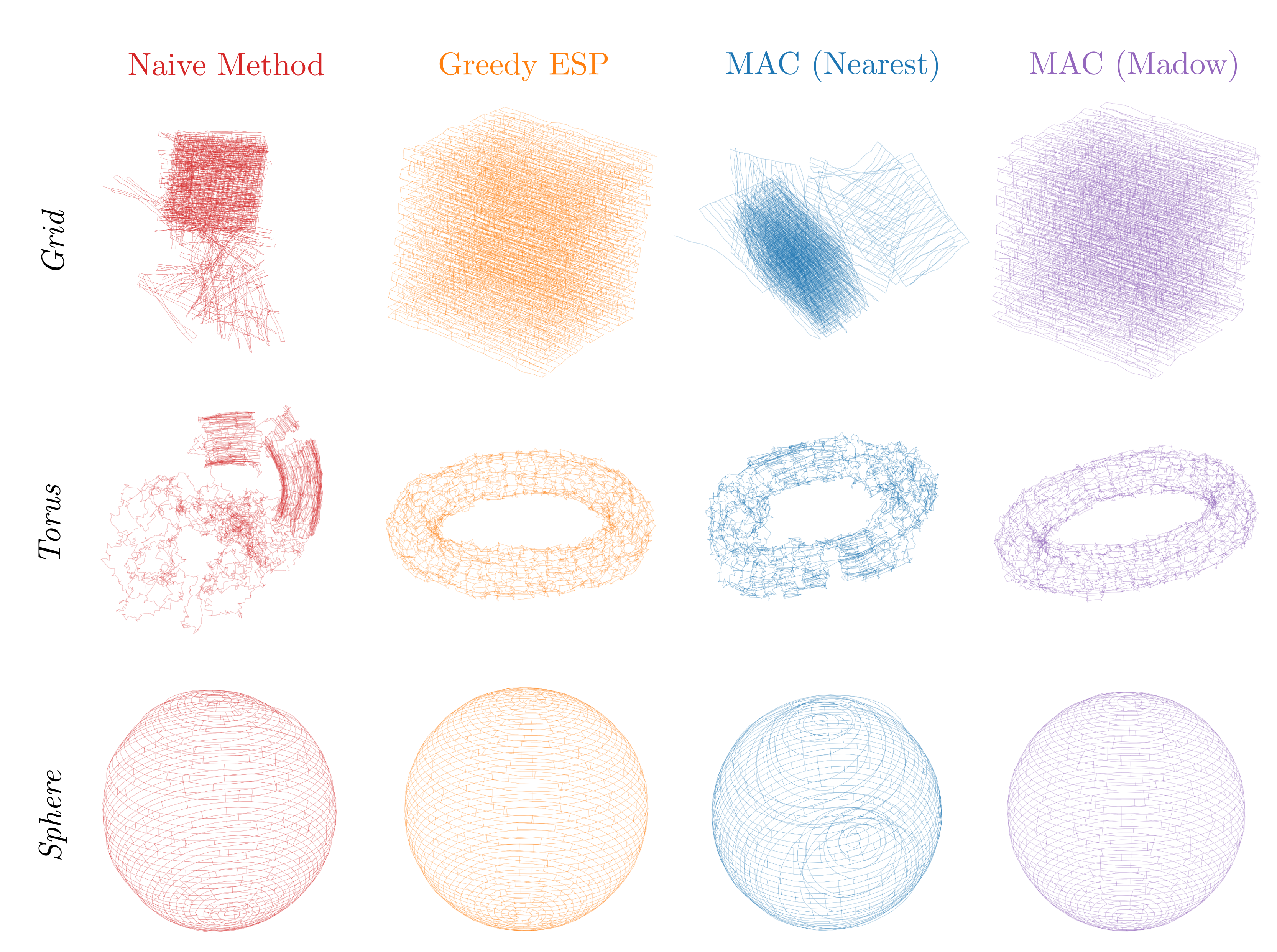
Figure 1: Qualitative results for 3D pose-graph sparsification. Pose-graph optimization results for the three 3D benchmark datasets after pruning all but 20% of the original loop closures using each method: (Top) Grid, (Middle) Torus, (Bottom) Sphere.

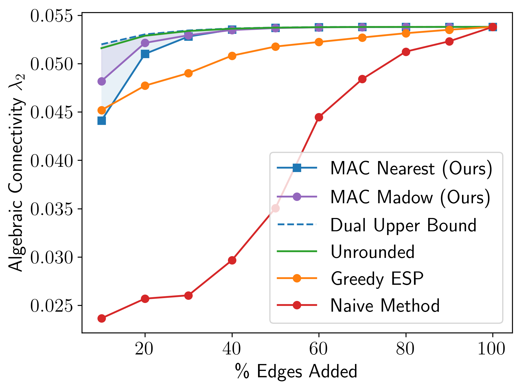
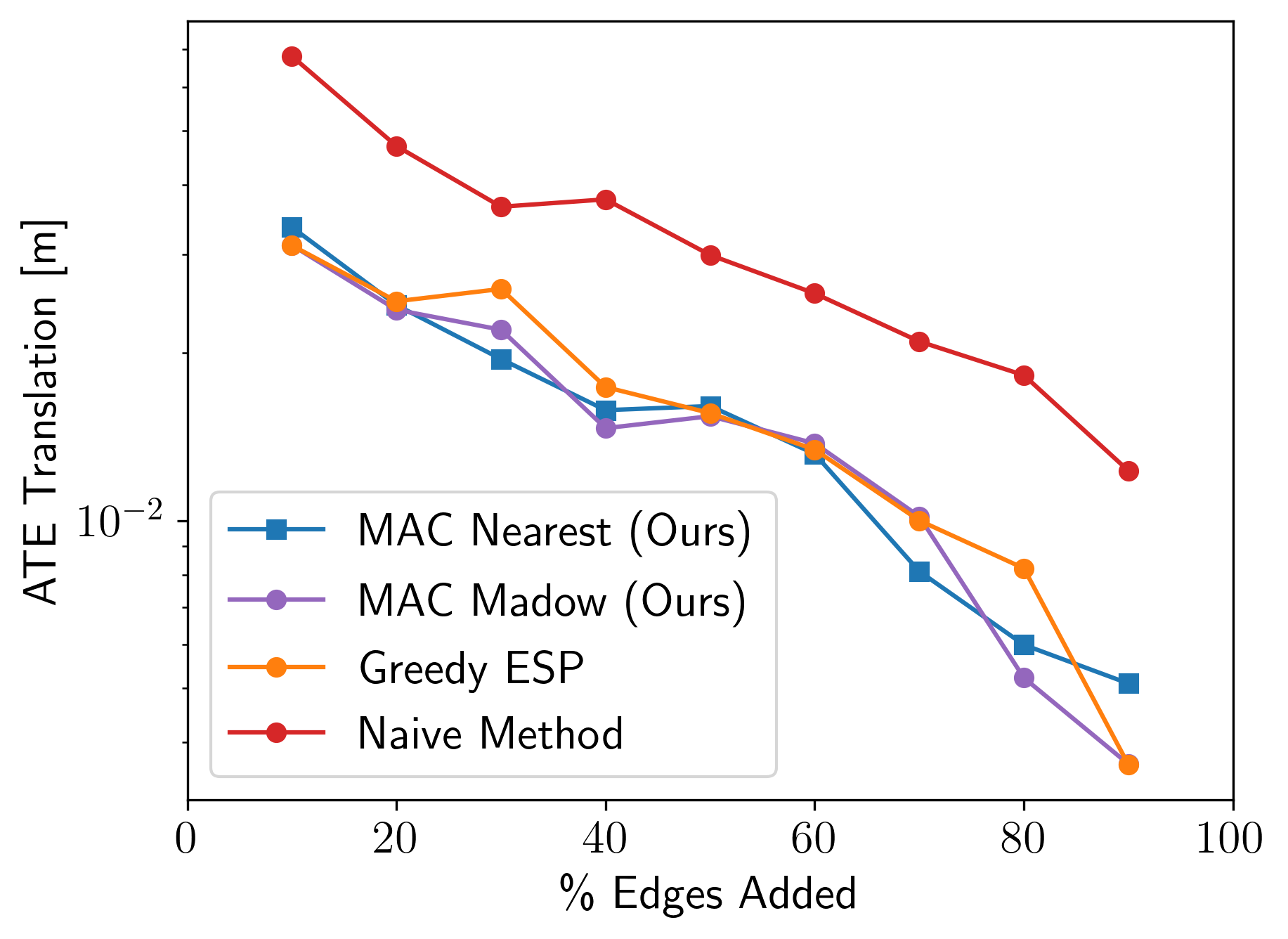
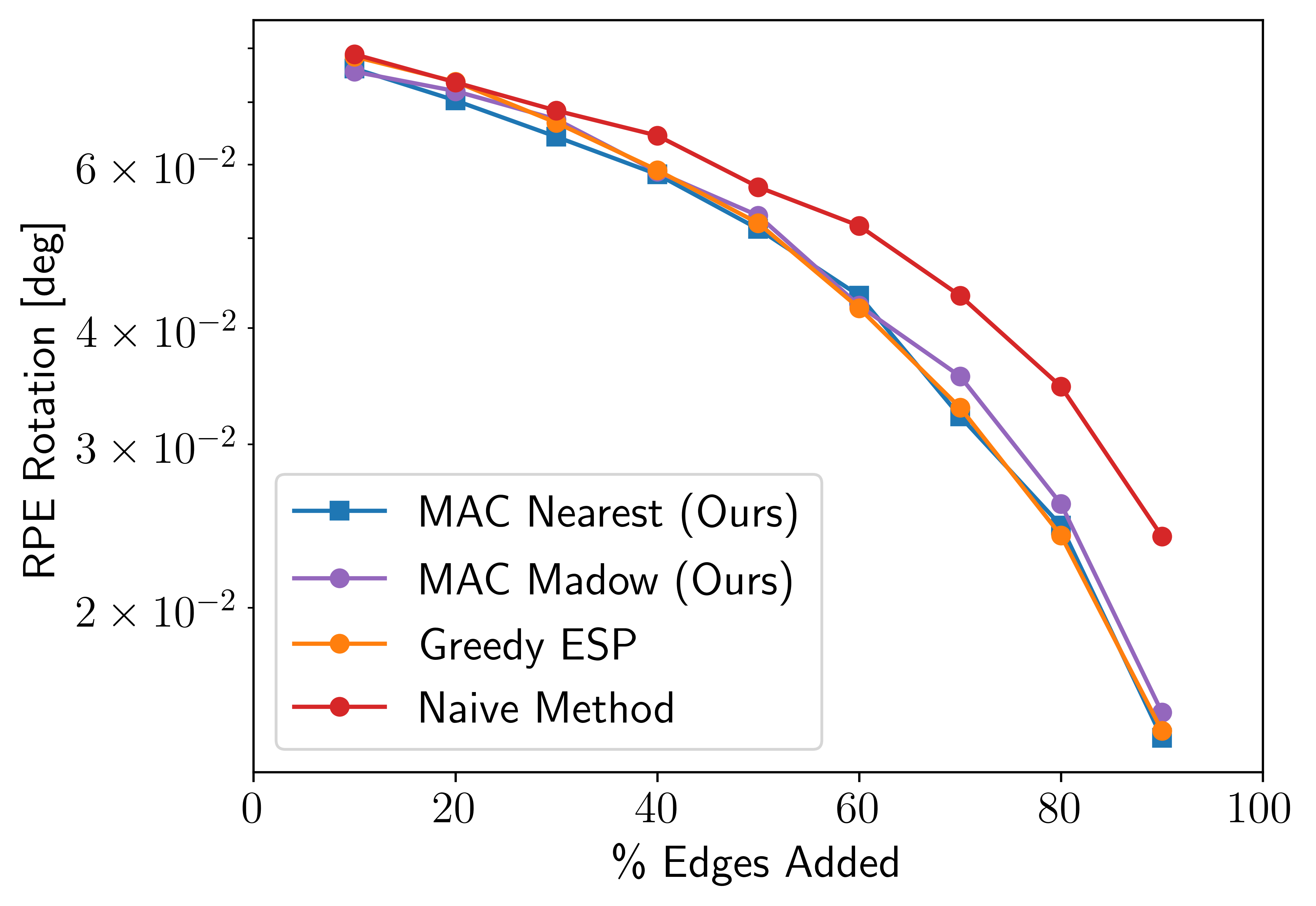
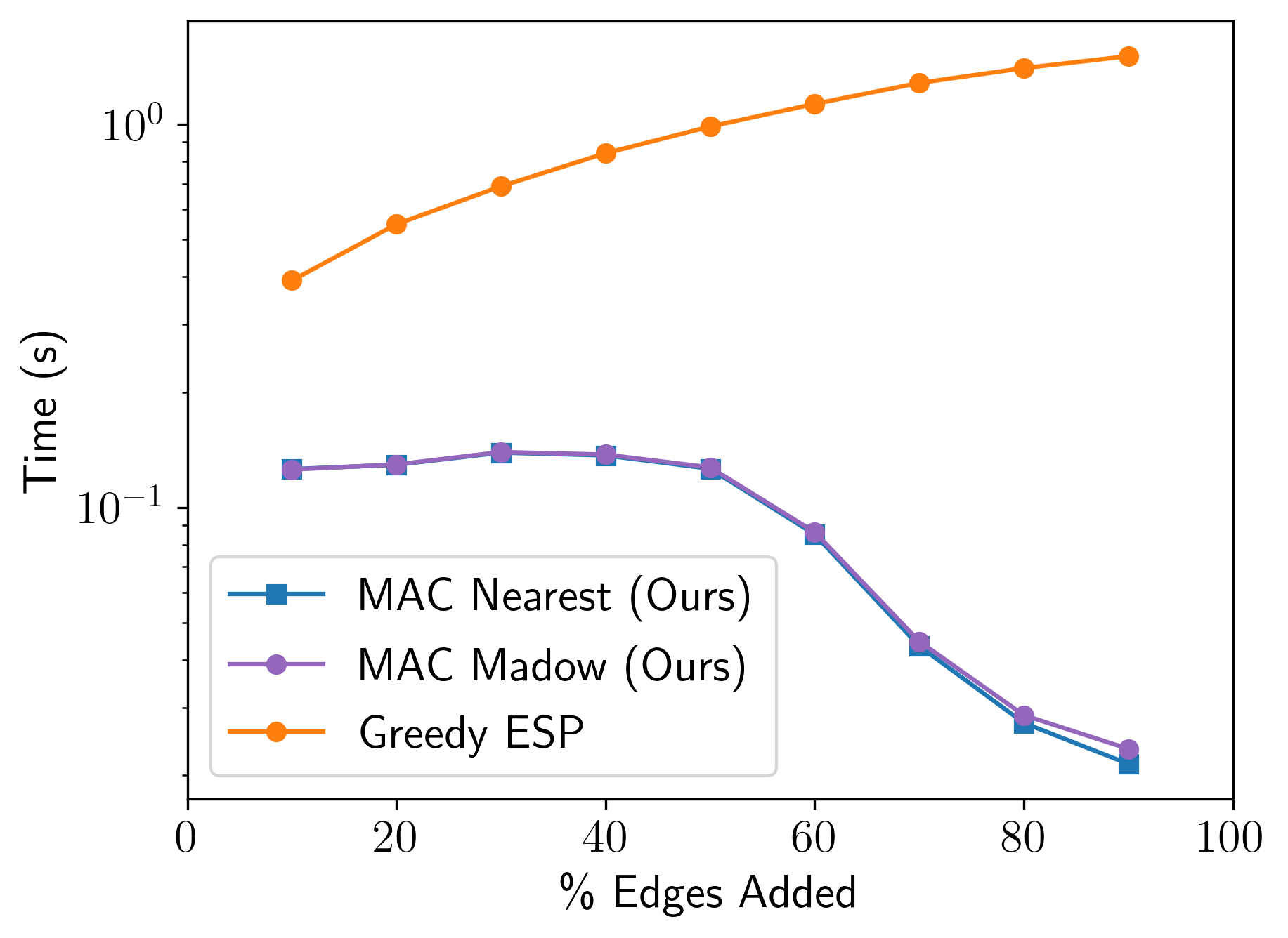
(a) Intel

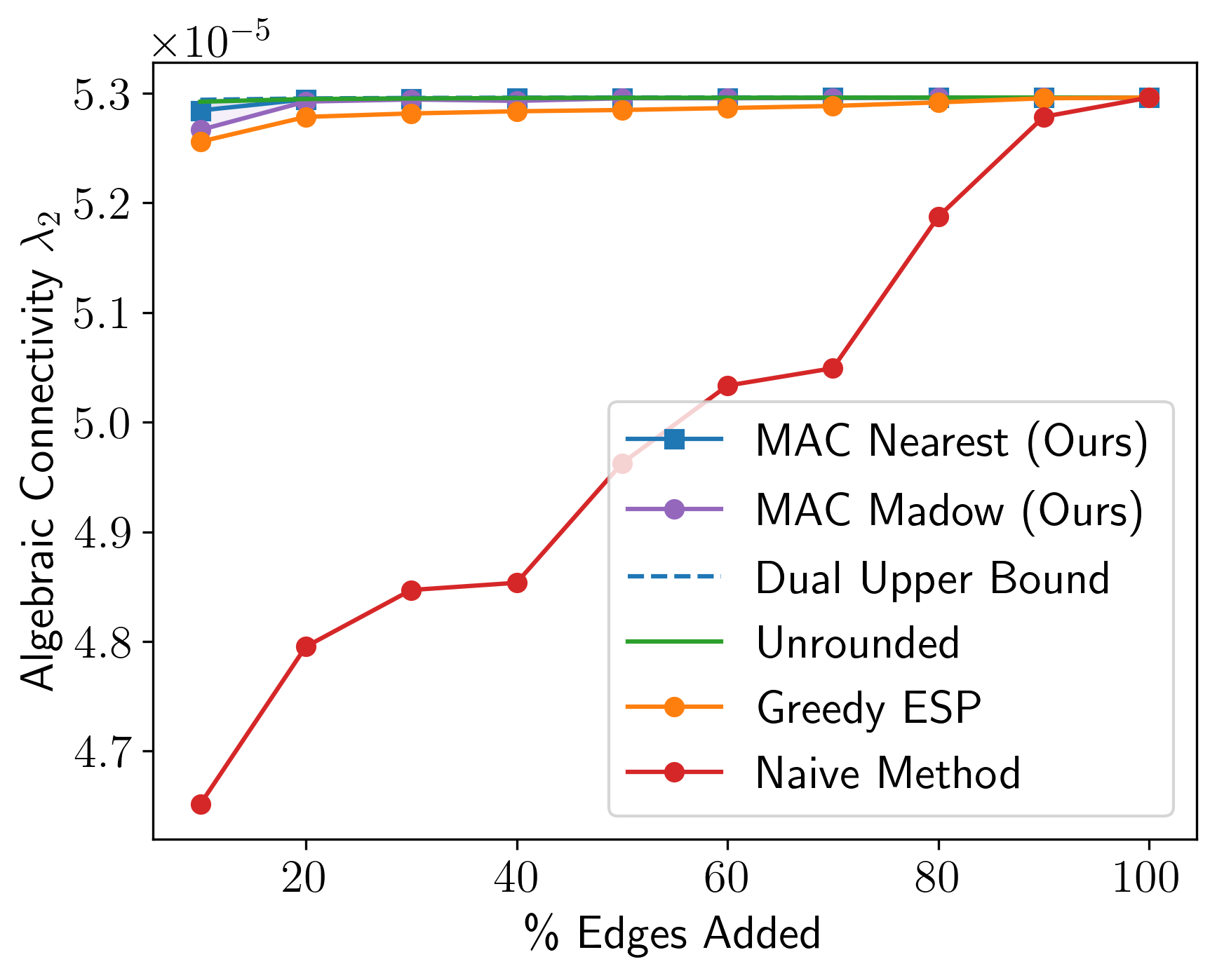
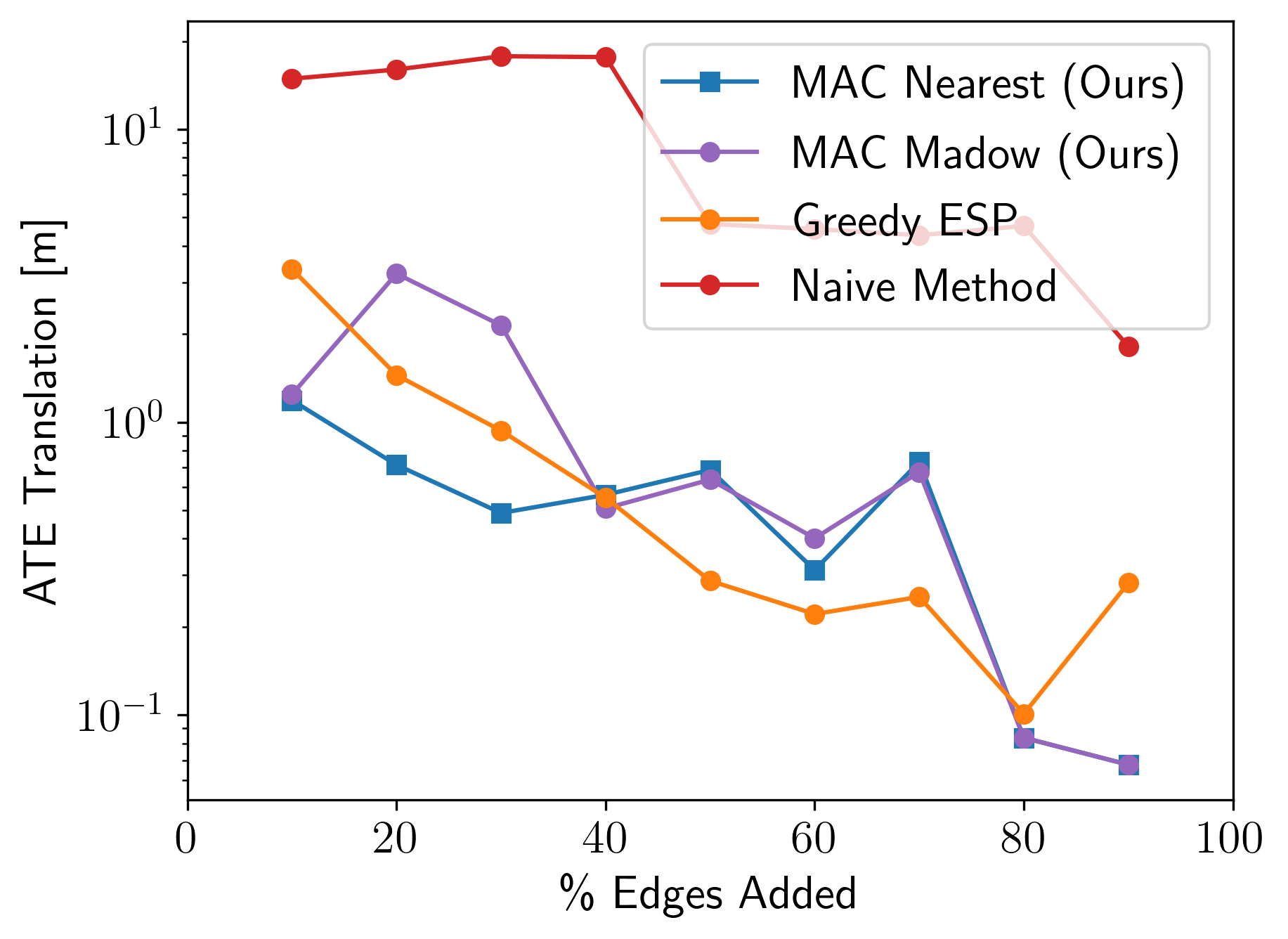
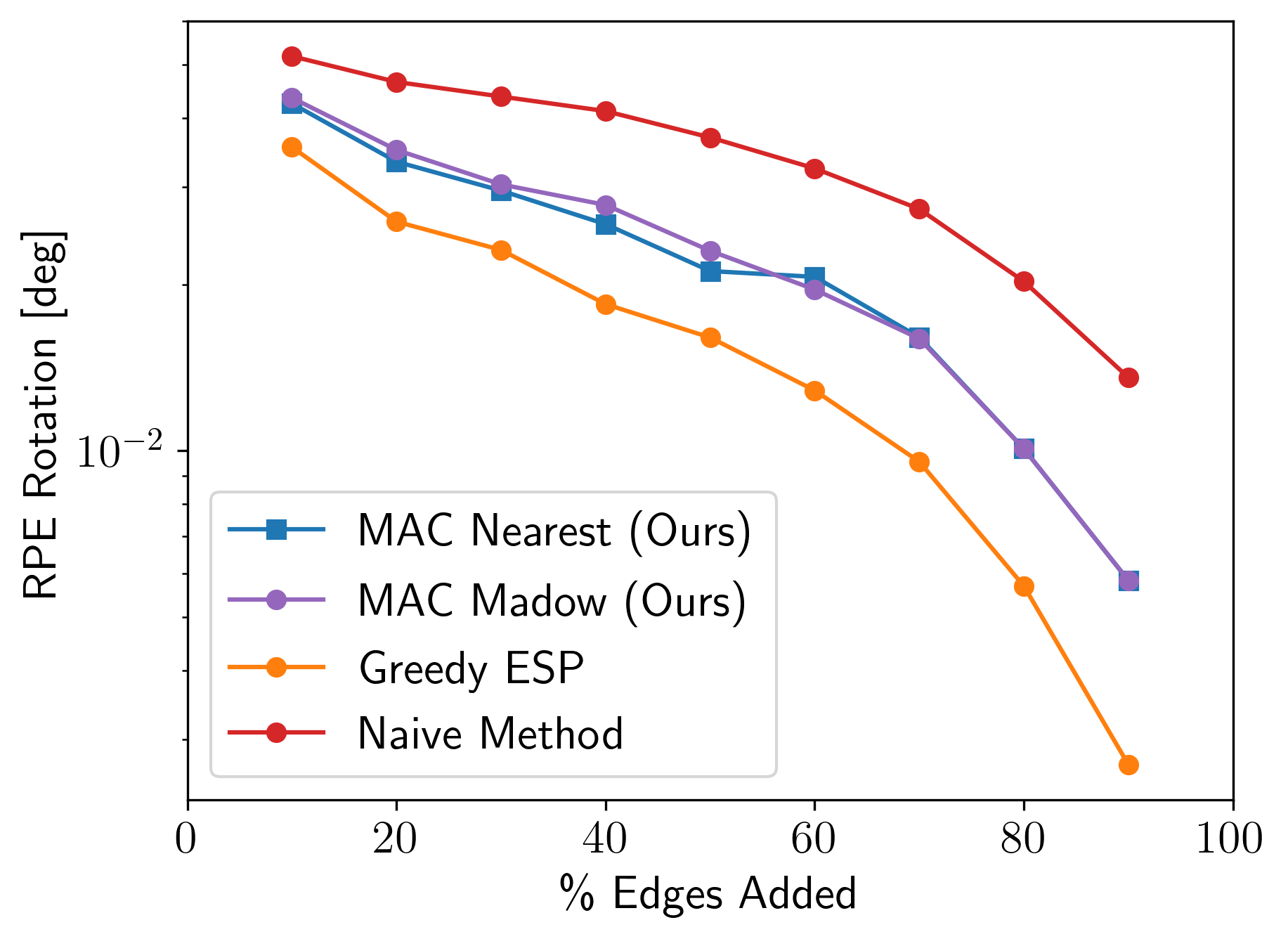
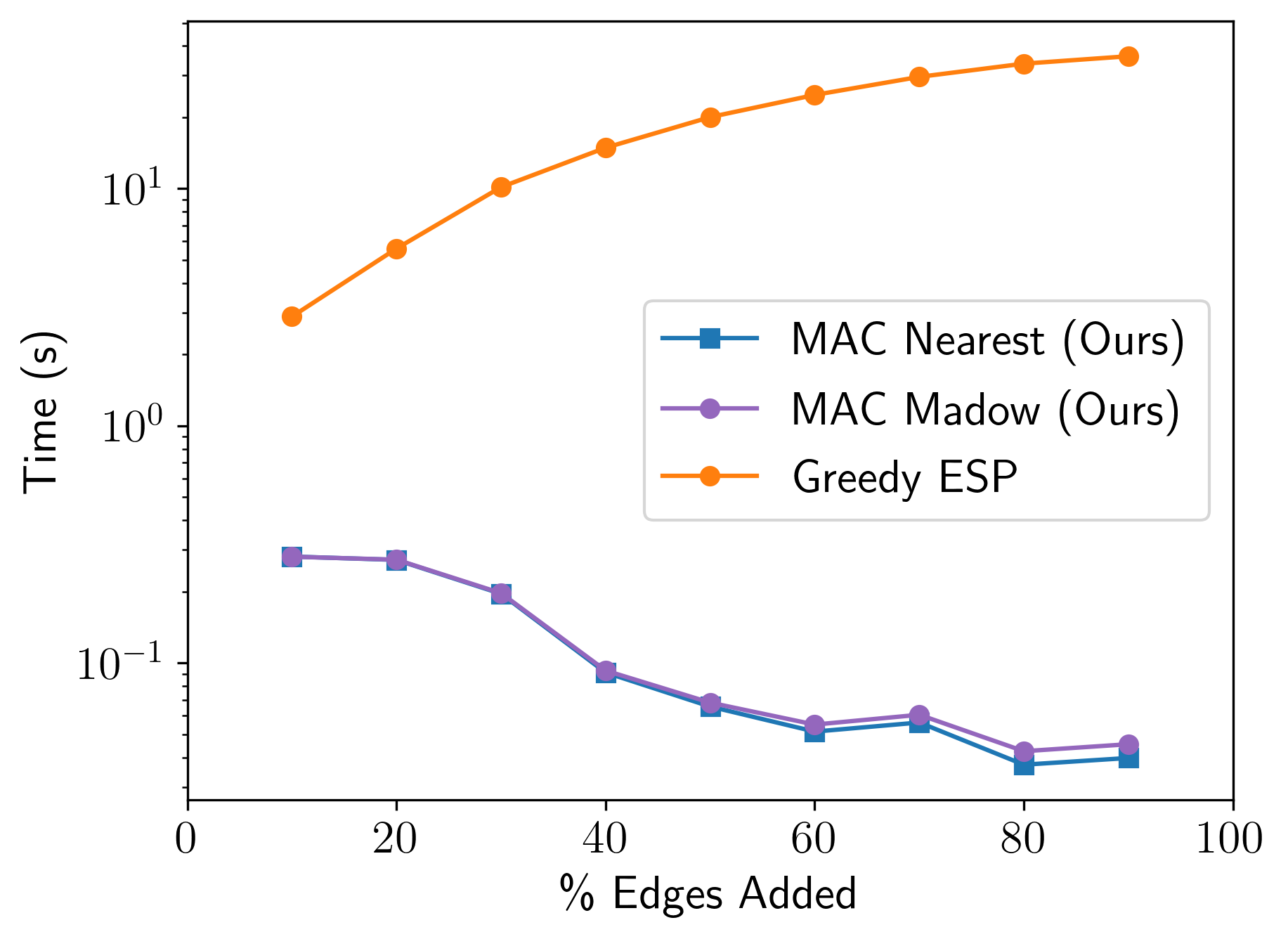
(b) AIS2Klinik

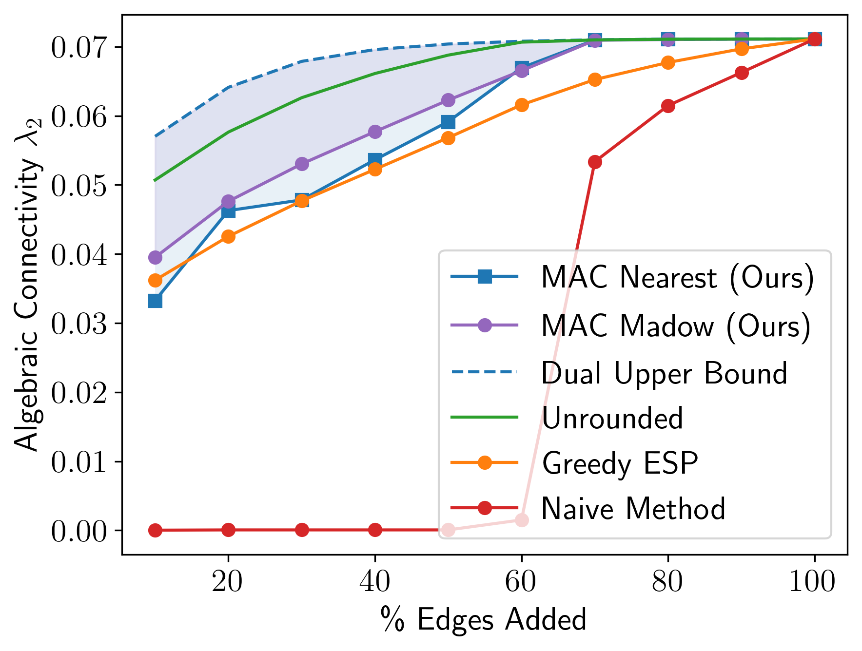
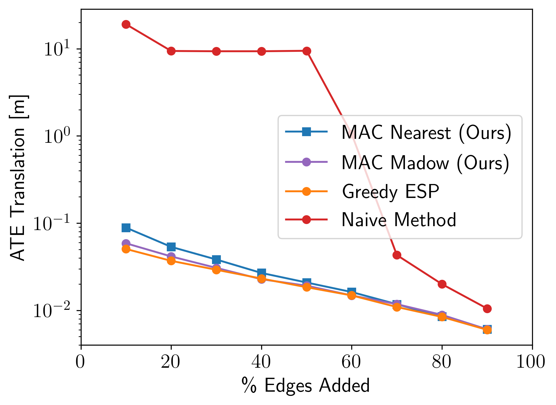
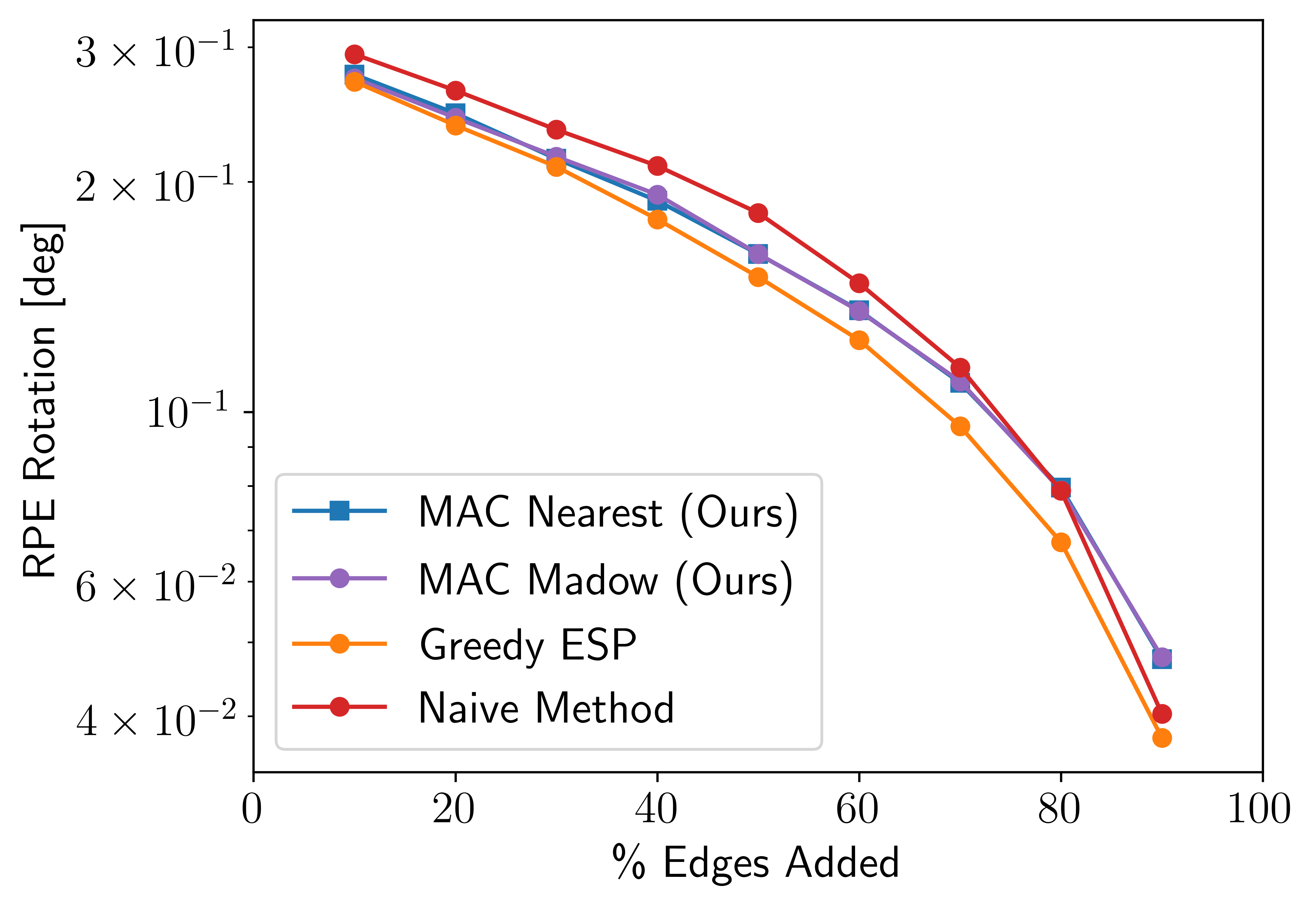
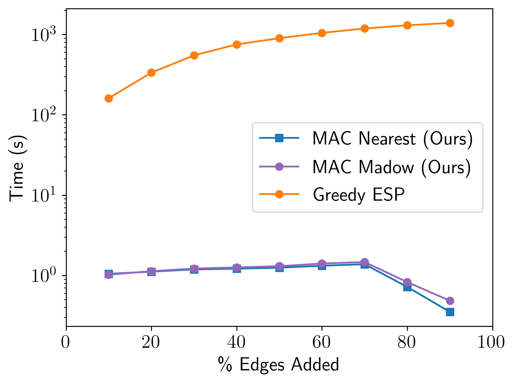
(c) City10K

Figure 2: Quantitative results for 2D pose-graph sparsification. Pose-graph optimization results for (a) the Intel dataset, (b) the AIS2Klinik dataset, and (c) the City10K dataset with varying degrees of sparsity (as percent of candidate edges added). Left to right: The algebraic connectivity of the graphs obtained using each method (larger is better) with the shaded regions indicating the suboptimality gap for each MAC rounding procedure, the mean translation error and relative rotation error compared to a maximum-likelihood estimate computed for the full graph, i.e. with all edges retained (smaller is better; note the logarithmic scale), and the computation time (logarithmic scale) for each approach. For 100% loop closures, both algorithms return immediately, so no computation time is reported.

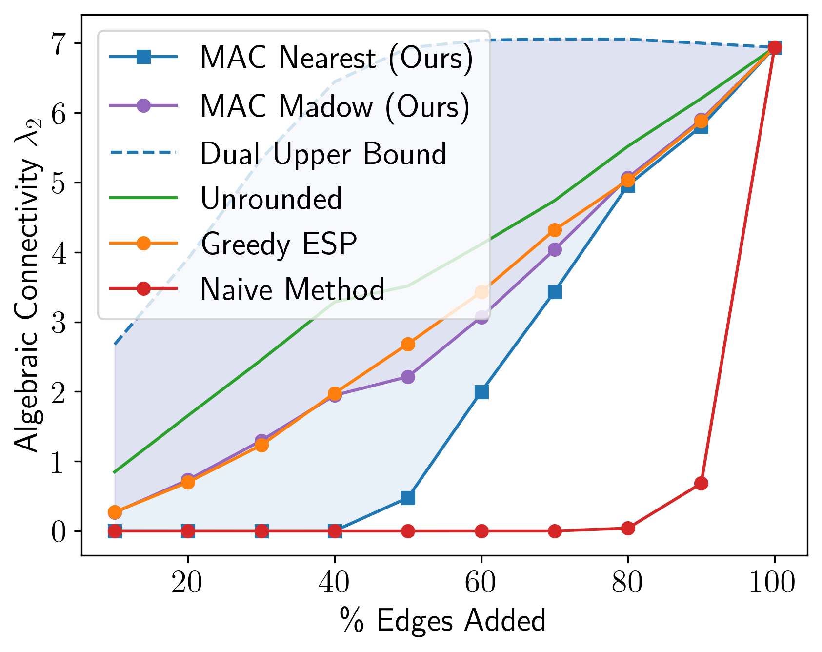
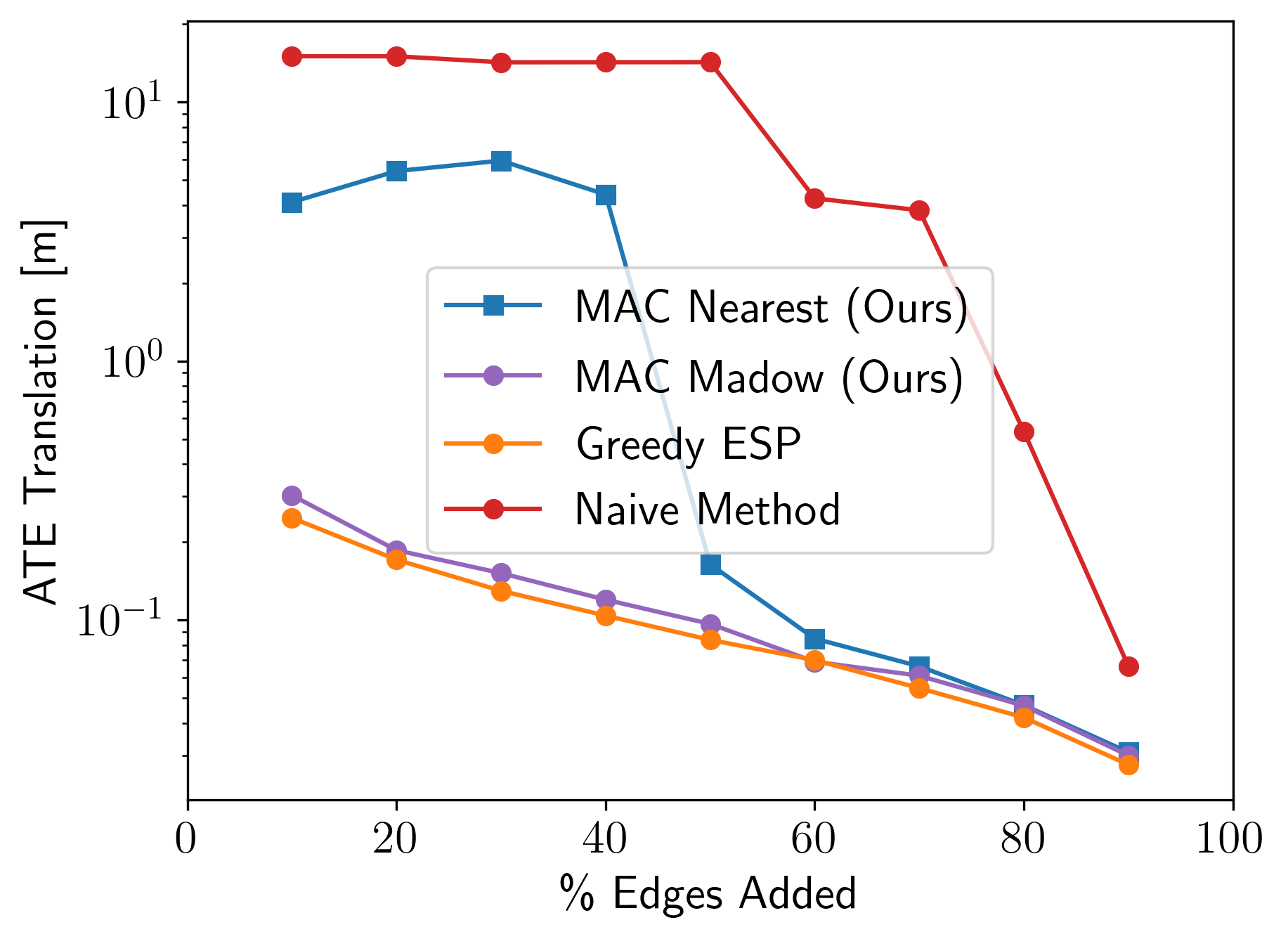
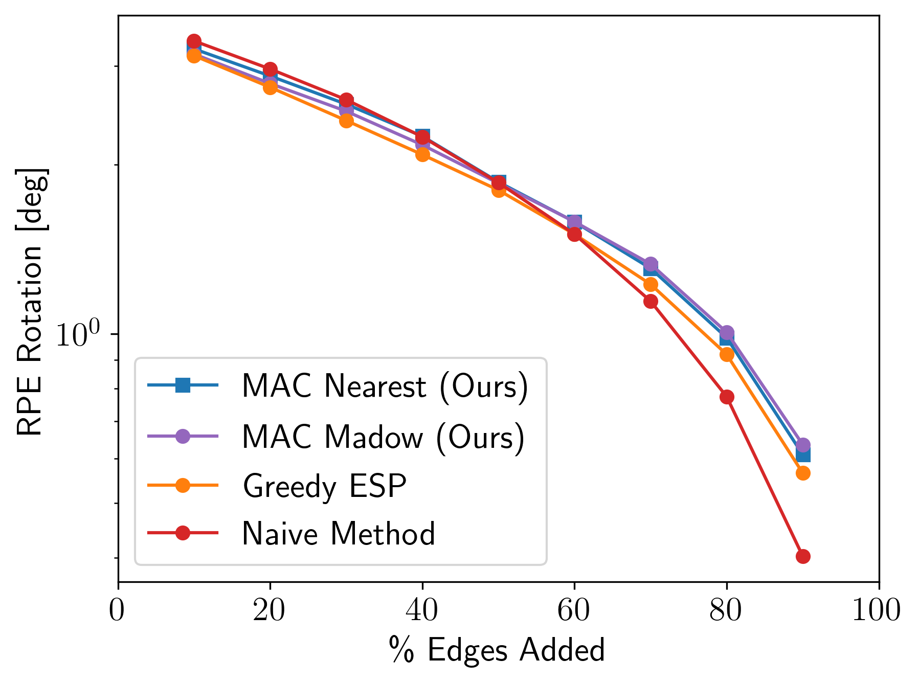
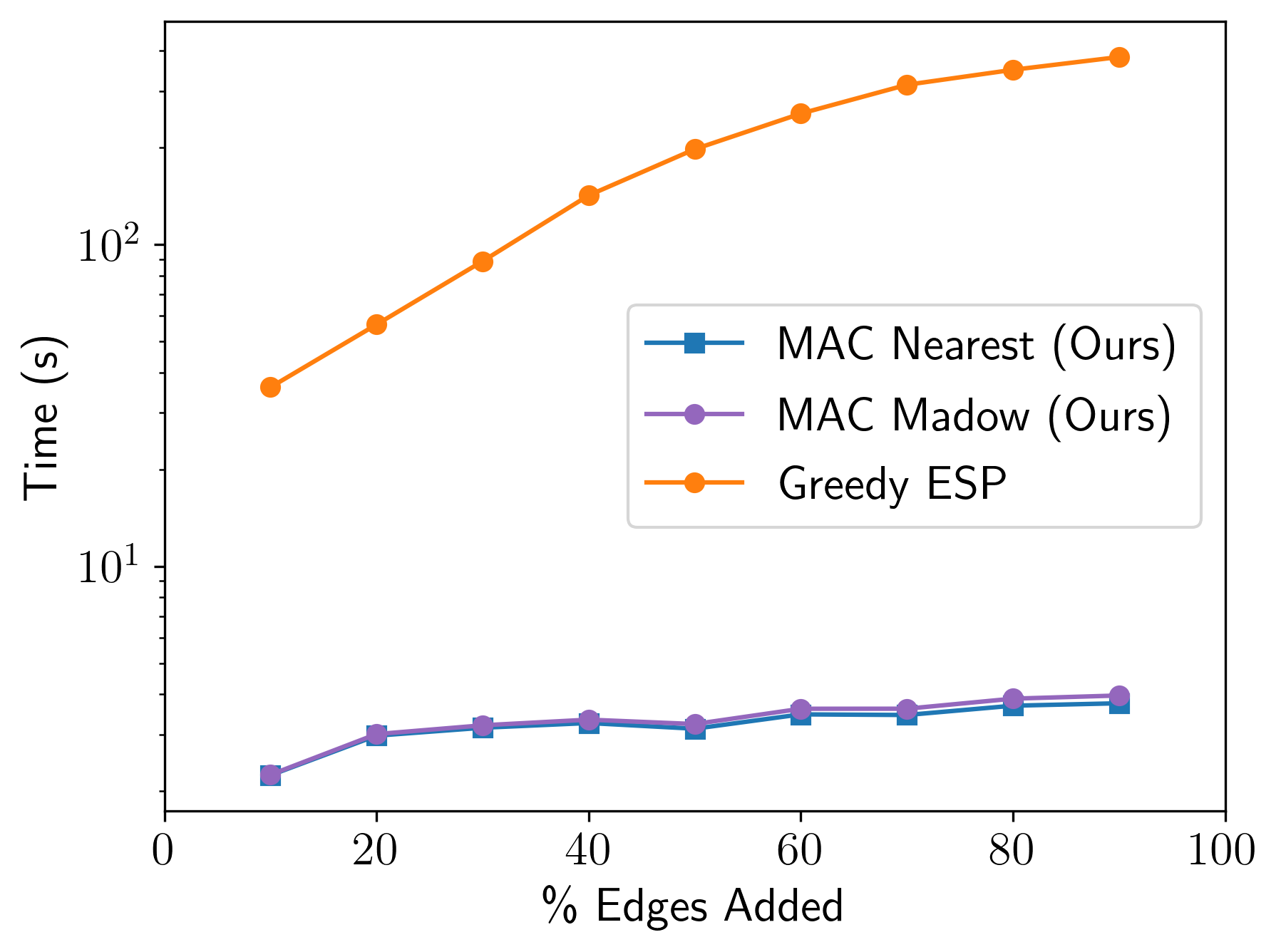
(a) Grid

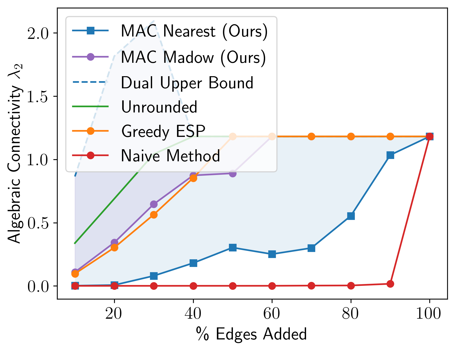
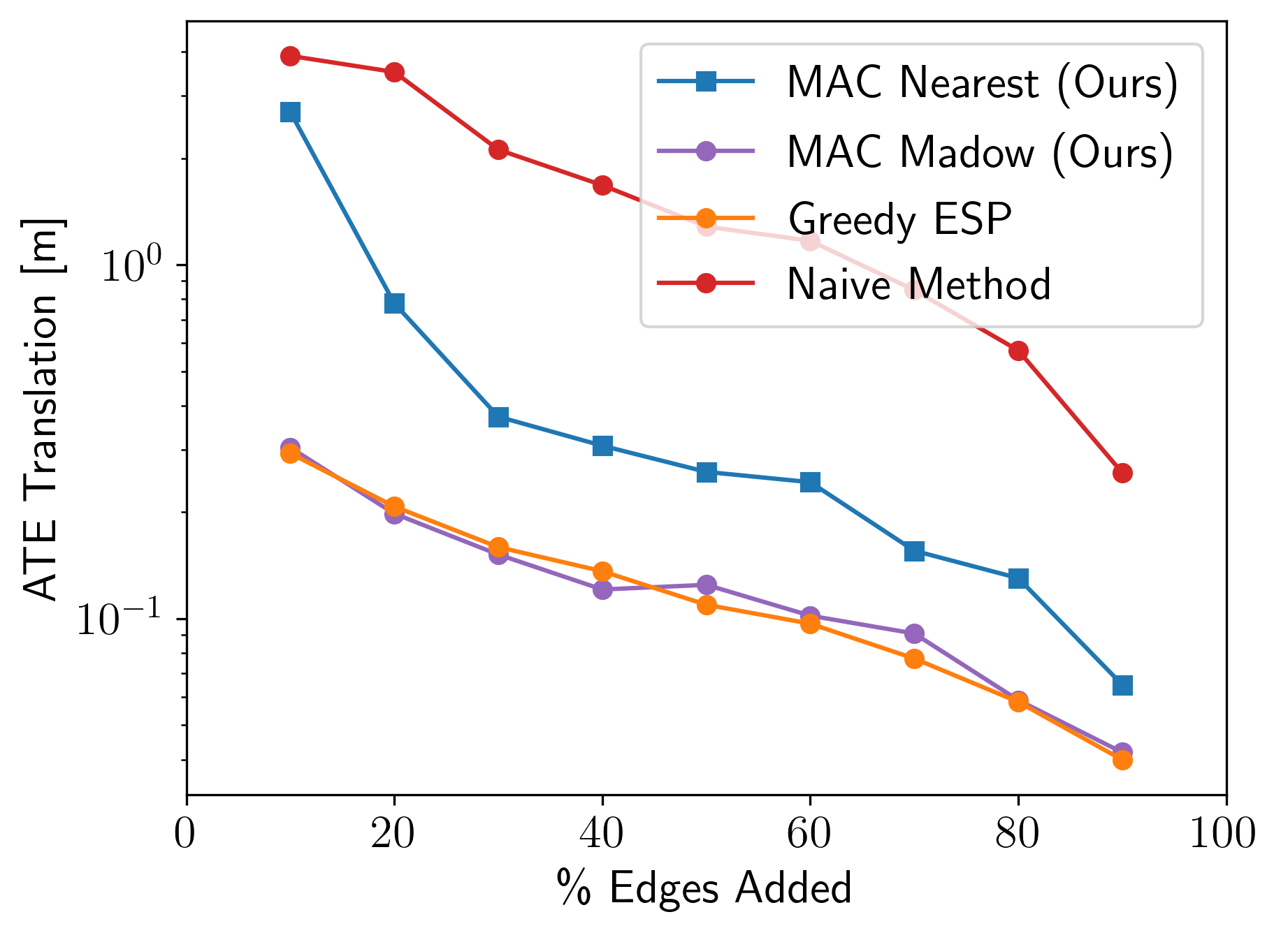
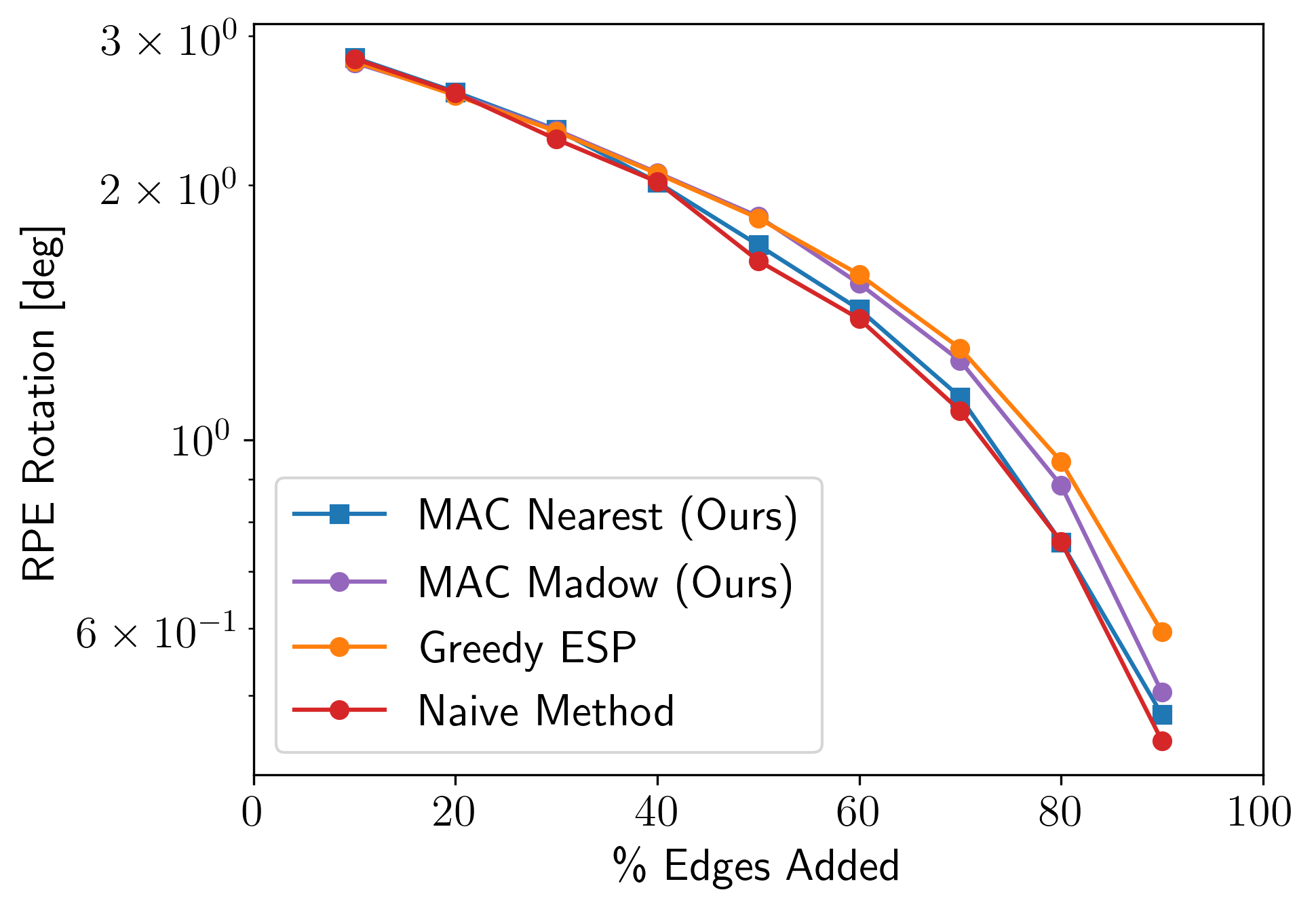
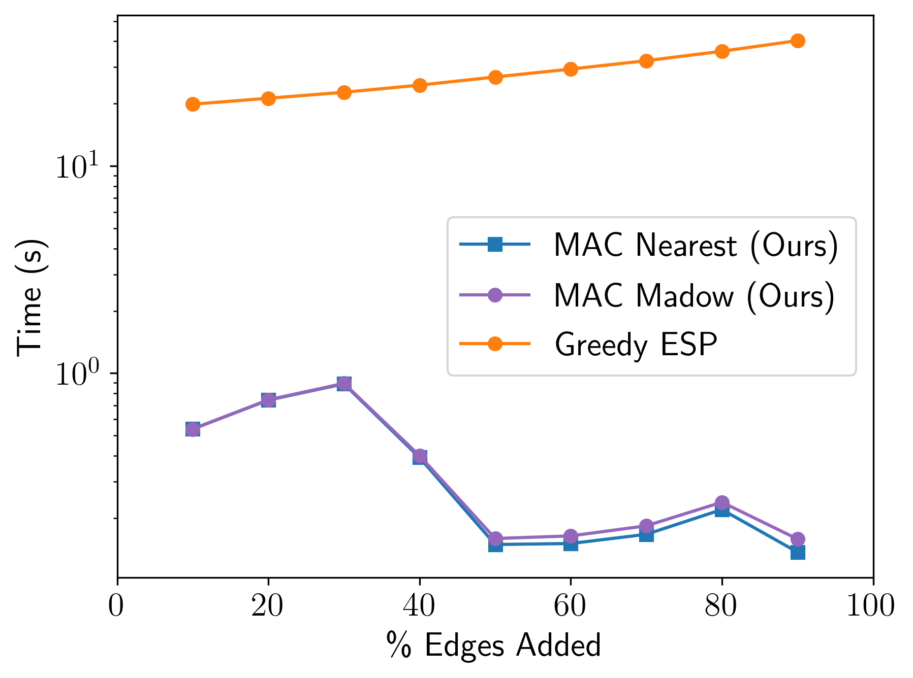
(b) Torus

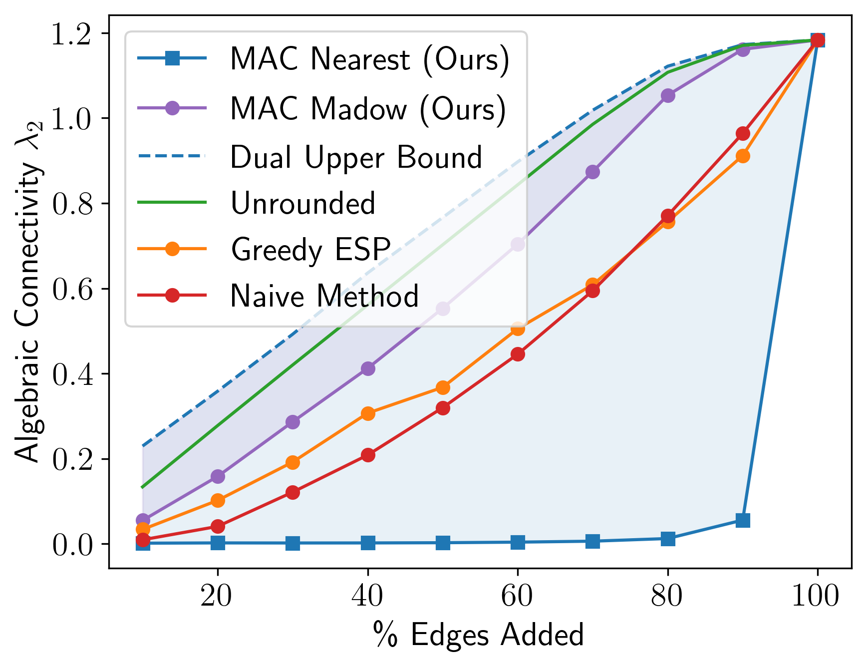
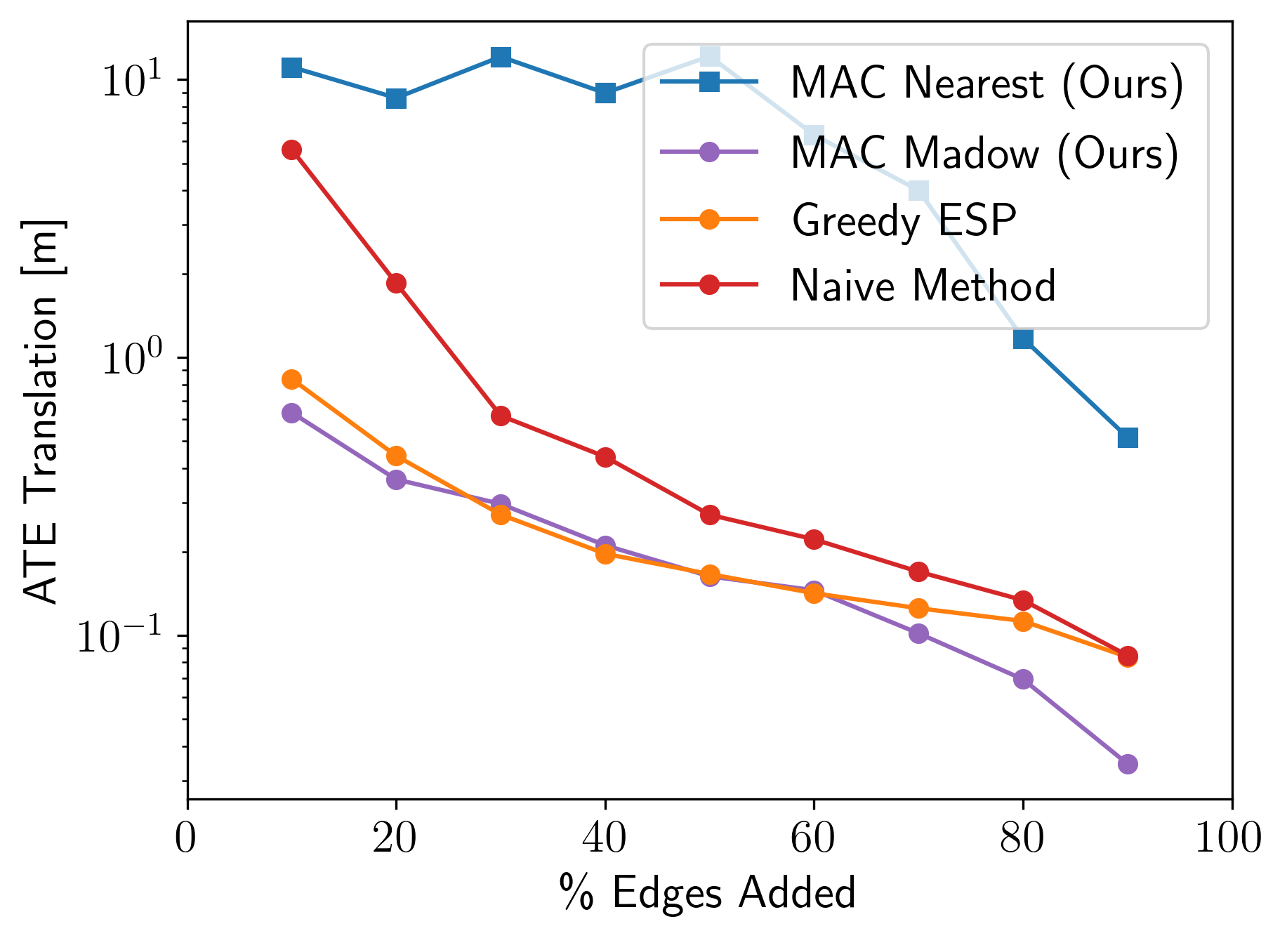
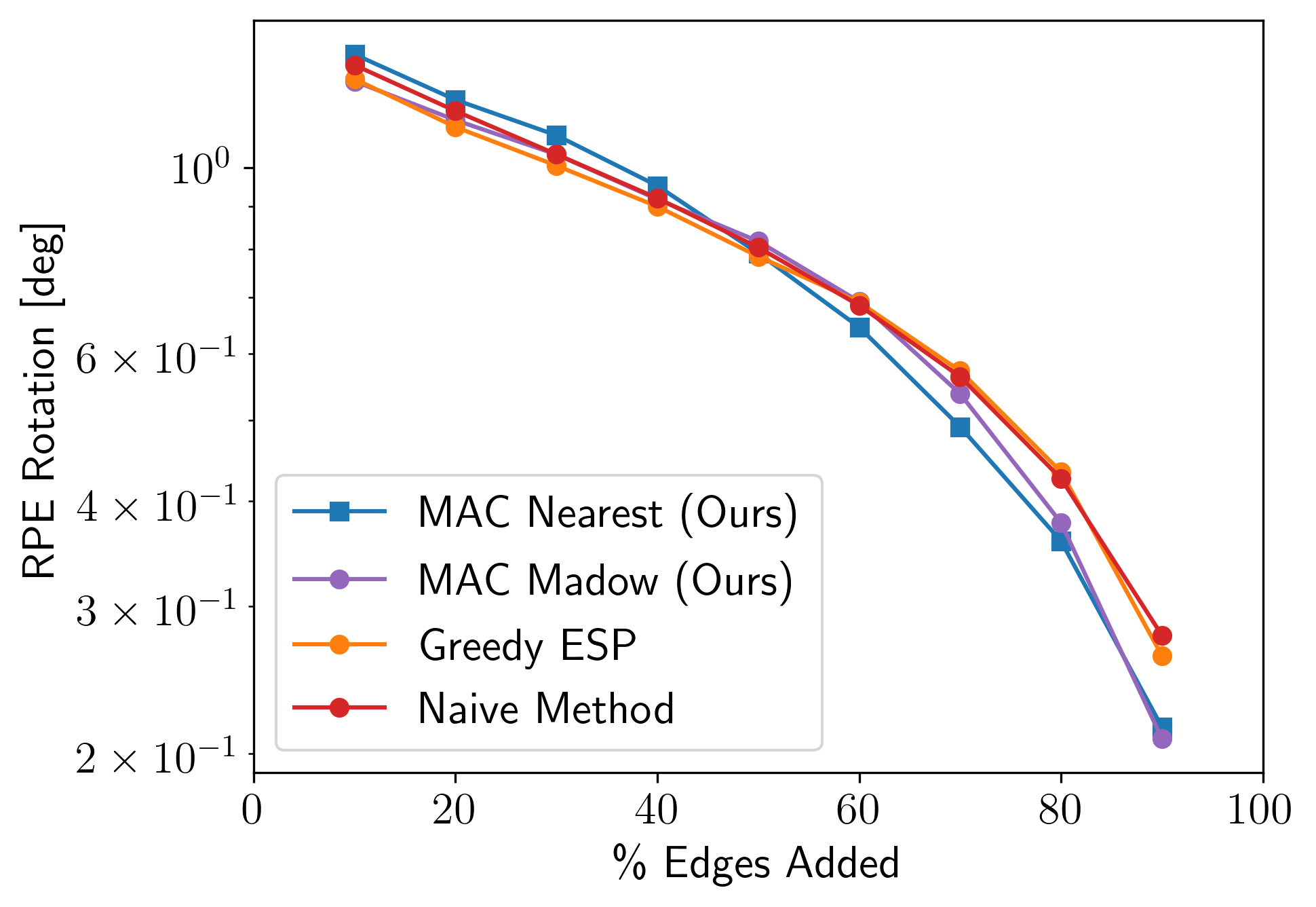
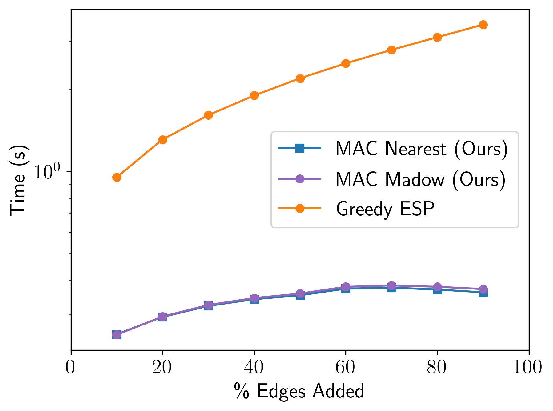
(c) Sphere

Figure 3: Quantitative results for 3D pose-graph sparsification. Pose-graph optimization results for (a) the Grid dataset, (b) the Torus dataset, and (c) the Sphere dataset with varying degrees of sparsity (as percent of candidate edges added). Left to right: The algebraic connectivity of the graphs obtained using each method (larger is better) with the shaded regions indicating the suboptimality gap for each MAC rounding procedure, the mean translation error and relative rotation error compared to a maximum-likelihood estimate computed for the full graph, i.e. with all edges retained (smaller is better; note the logarithmic scale), and the computation time (logarithmic scale) for each approach. For 100% loop closures, both algorithms return immediately, so no computation time is reported.

Dataset	# Nodes	# Candidate Edges
Intel	1728	785
Sphere	2500	2500
Torus	5000	4049
Grid	8000	14237
City10K	10000	10688
AIS2Klinik	15115	1614

TABLE I: Summary of the datasets used in our experiments.

We implemented the MAC algorithm in Python and all computational experiments were performed on a 2.4 GHz Intel i9-9980HK CPU. For computation of the Fiedler value and the corresponding vector, we use TRACEMIN-Fiedler [38, 39]. Where in our previous work [16] we used an LU decomposition as a subprocedure of TRACEMIN-Fiedler, in this paper we instead use the Cholesky decomposition provided by Suitesparse [43]. Both options are exposed by the MAC library. We have also improved the computational efficiency of calculating the Fiedler vectors required to form the direction-finding subproblems in each iteration of the Frank-Wolfe method (Algorithm 1): since the Fiedler vectors obtained in subsequent iterations are often close, warm-starting the TRACEMIN-Fiedler method using the Fiedler vector computed in the previous iteration can result in substantial computational savings. In all experiments, we run MAC for a maximum of 20 iterations, or when the duality gap in equation (25) reaches a tolerance of $10^{-8}$.

In the following sections, we present experimental results using MAC for sparsification of benchmark pose-graph SLAM datasets, as well as on real data from the University of Michigan North Campus Long-Term (NCLT) Dataset [44]. In all of our experiments, we use odometry edges (between successive poses) to form the base graph and loop closure edges as candidate edges. We consider selection of $10\%,20\%,\ldots,100\%$ of the candidate loop closure edges in the sparsification problem.

We compare both of the rounding procedures (from Section IV-C), along with a naïve heuristic method which selects simply the subset of candidate edges with the largest edge weights. This simple heuristic approach serves two purposes: First, it provides a baseline, topology-agnostic approach to demonstrate the impact of considering graph connectivity in a sparsification procedure; second, we use this method to provide a sparse initial estimate to our algorithm. We also compare our approach with the “greedy edge selection problem” (Greedy ESP) algorithm of Khosoussi et al. [20] for approximate D-optimal graph sparsification. In an effort to make the comparison as fair as possible, we have implemented our own version of the Greedy ESP algorithm in Python which makes use of lazy evaluation [45, 46], as well as incremental, sparse Cholesky factorization, as proposed in [20].

V-A Benchmark pose-graph SLAM datasets

We evaluated the MAC algorithm using several benchmark pose-graph SLAM datasets. We present results on six datasets in this paper (summarized in Table I). Three of the datasets we considered (Intel, AIS2Klinik, and City10K) represent 2D SLAM problems (corresponding to Problem 1 with $d=2$), and the remaining three (Sphere, Torus, and Grid) represent 3D SLAM problems. The Intel dataset and the AIS2Klinik dataset are both obtained from real data, while the remaining datasets are synthetic. We apply MAC to sparsify each graph to varying degrees of sparsity and apply SE-Sync [10] to compute globally optimal estimates of robot poses for the graphs with edge sets selected by each method.

Figure 1 gives a qualitative comparison of the results from our approach as compared with the baselines on each of the 3D benchmark datasets we considered. Interestingly, the Greedy ESP method and MAC with randomized rounding (denoted MAC (Madow)) produce qualitatively very similar results, despite optimizing for different criteria. Perhaps more surprisingly, MAC with the “nearest neighbors” style of rounding (denoted MAC (Nearest)) fails quite dramatically on the Grid dataset and similarly on the Torus dataset. We had not observed this phenomenon in our prior work [16] where we had only thus far applied the method to 2D datasets. This may be a consequence of the synthetic construction of these datasets (and we have not observed similar failures on any real data). In particular, each of these datasets is constructed in a manner that produces symmetries in the graph topology. We do not explicitly consider the presence of symmetries in our objective (though if these symmetries are known a priori, it is possible to do so in principle, see, e.g. related discussion in [21]). In problems exhibiting symmetry, there may be multiple solutions $x^{*}_{1},\ldots,x^{*}_{p}$ to Problem 2 that achieve the global minimum. In these cases, the concavity of the objective in (10) implies that the average $\bar{x}\triangleq(1/p)\sum_{i}x^{*}_{i}$ of these solutions will always achieve an objective value that is at least as good for the relaxed problem (Problem 10) as that attained by the $x_{i}$ themselves. In such cases, applying a simple top-$K$ rounding procedure may select edges that belong to multiple distinct optima $x^{*}_{i}$, $x^{*}_{j}$. On the other hand, because the greedy method (by construction) builds its solutions sequentially (by selecting one edge at a time), as soon as a distinguishing edge belonging to one of the distinct optima has been added to the solution under construction (thus breaking the symmetry), the greedy method is likely to prefer selecting other edges belong to that specific configuration in subsequent iterations. We conjecture that the randomness introduced in the Madow sampler helps to achieve a similar kind of symmetry breaking when rounding relaxed solutions of Problem 10.

For a quantitative comparison of each method, we report three performance measures: (1) the algebraic connectivity $\lambda_{2}(L(x))$ of the graphs determined by each edge selection $x$; (2) the translational part of the absolute trajectory error (ATE) between the SLAM solution computed from the sparsified pose graph and the solution computed using the full pose graph (i.e. keeping 100% of the edges); and (3) the average of the rotational component of the relative pose error. We also report the computation time required to obtain a solution for each method.

Figure 2 summarizes our quantitative results on each 2D benchmark dataset. Our approach consistently achieves better connected graphs (as measured by the algebraic connectivity). In most cases, a maximum of 20 iterations was enough to achieve solutions to the relaxation with algebraic connectivity very close to the dual upper bound (and therefore nearly globally optimal).

Beyond providing high-quality sparse measurement graphs, our approach is also fast. For the Intel dataset, all solutions were obtained in less than 250 milliseconds. Sparsifying the (larger) AIS2Klinik dataset required up to 700 ms, but only around 100 ms when larger edge selections were allowed. In those cases, the duality gap tolerance was reached and optimization could terminate. The largest dataset (in terms of candidate edges) is the City10K dataset, with over 10000 loop closure measurements to select from. Despite this, our approach produces near-optimal solutions in under 2 seconds.

With respect to the suboptimality guarantees of our approach, it is interesting to note that on both the Intel and City10K datasets, the rounding procedure introduces fairly significant degradation in algebraic connectivity - particularly for more aggressive sparsity constraints. In these cases, it seems that the Boolean relaxation we consider leads to fractional optimal solutions. It is not clear in these cases whether the integral solutions obtained by rounding are indeed suboptimal for the Problem 2, or whether this is a consequence of the integrality gap between global optima of the relaxation and of Problem 2.

Figure 3 summarizes our quantitative results on each of the 3D benchmark pose-graph optimization datasets. As previously discussed, the MAC (Nearest) method, which uses the “nearest neighbors” rounding procedure, struggles on these synthetic datasets, whereas the MAC (Madow) approach using the randomized rounding procedure incurs significantly less degradation in connectivity compared to the unrounded solution to the relaxation. Interestingly, on both the Grid and Torus datasets, we also observe that the dual upper bounds computed during optimization can be quite loose. This is in contrast to the 2D datasets, where MAC fairly consistently achieved solutions, at least to the relaxation, which were quite close in algebraic connectivity to the dual upper bounds.

V-B Real multi-session SLAM data

In this section, we evaluate the performance of MAC on real large-scale multi-session data from the University of Michigan North Campus Long-Term Dataset [44]. To generate pose graphs, we processed LiDAR data from three sessions using Fast-LIO2 [47] for odometry with loop closure measurements generated based on ScanContext [48]. For loop closures between sessions, we use DiSCo-SLAM [49]. We processed each session in order, so loop closures are generated from the second session to the first as well as from the third session to both the first and second sessions. This entire procedure was performed offline as a preprocessing step to construct multi-session pose graphs. We then sparsified loop closures in this dataset using MAC (making no distinction between inter- and intra-session loop closures). We use the same metrics for comparison as in our evaluation on benchmark pose-graph SLAM datasets, but trajectory errors here are computed with respect to the ground truth, rather than the optimal solution for the full graph.

An interesting difference between this dataset and the benchmark pose-graph optimization datasets we considered in the previous section is that the loop closures generated using ScanContext can be corrupted by outliers. In our application, the MAC algorithm itself does not account for any possibility of outliers. In these examples, it was possible to mitigate the influence of outlier loop closures simply by using a Cauchy robust kernel for all loop closure measurements while applying MAC without modification.

Qualitative comparisons of the results for the different methods are provided in Fig. 4 and Fig. 5. Both figures show the case where $20\%$ of the loop closures are retained. Figure 4 provides a top-down view of the LiDAR point clouds reconstructed based on the pose estimates for graphs obtained using each sparsification method. MAC (with either rounding approach) and the Greedy ESP method provide results that are nearly indistinguishable visibly, whereas the naïve baseline fails to accurately anchor the trajectories from different sessions relative to one another. The offset trajectories visualized in Figure 5 give a closer look at this phenomenon. The naïve method achieves high connectivity between some parts of the three sessions, but poor connectivity in others. In contrast, the solution obtained by MAC appears to provide a more uniform distribution of loop closures across the trajectories.

The corresponding quantitative comparison is given in Figure 6. The comparison of the algebraic connectivity of each solution once again demonstrates a slight degradation of solution quality when using “nearest neighbors” rounding approach. These solutions similarly perform worse in terms of trajectory error metrics. Notably, MAC (Madow) produces rounded solutions whose algebraic connectivity is numerically almost identical to the unrounded solutions. This suggests that the solution to the relaxation for this dataset is very close to the feasible set for the original problem. Unfortunately, since we did not achieve convergence of the objective value and the dual upper bound, we cannot verify the optimality of these solutions. It is also interesting that the Greedy ESP method achieves an algebraic connectivity that is extremely close to that of MAC (Madow) across all edge budgets. This is reflected in the trajectory errors as well, where Greedy ESP and MAC (Madow) are almost indistinguishable in terms of trajectory error (with MAC (Madow) occasionally performing marginally better in terms of translation error and Greedy ESP occasionally providing lower rotation errors). However, MAC is able to achieve these results two to three orders of magnitude faster than Greedy ESP, depending upon the edge budget.

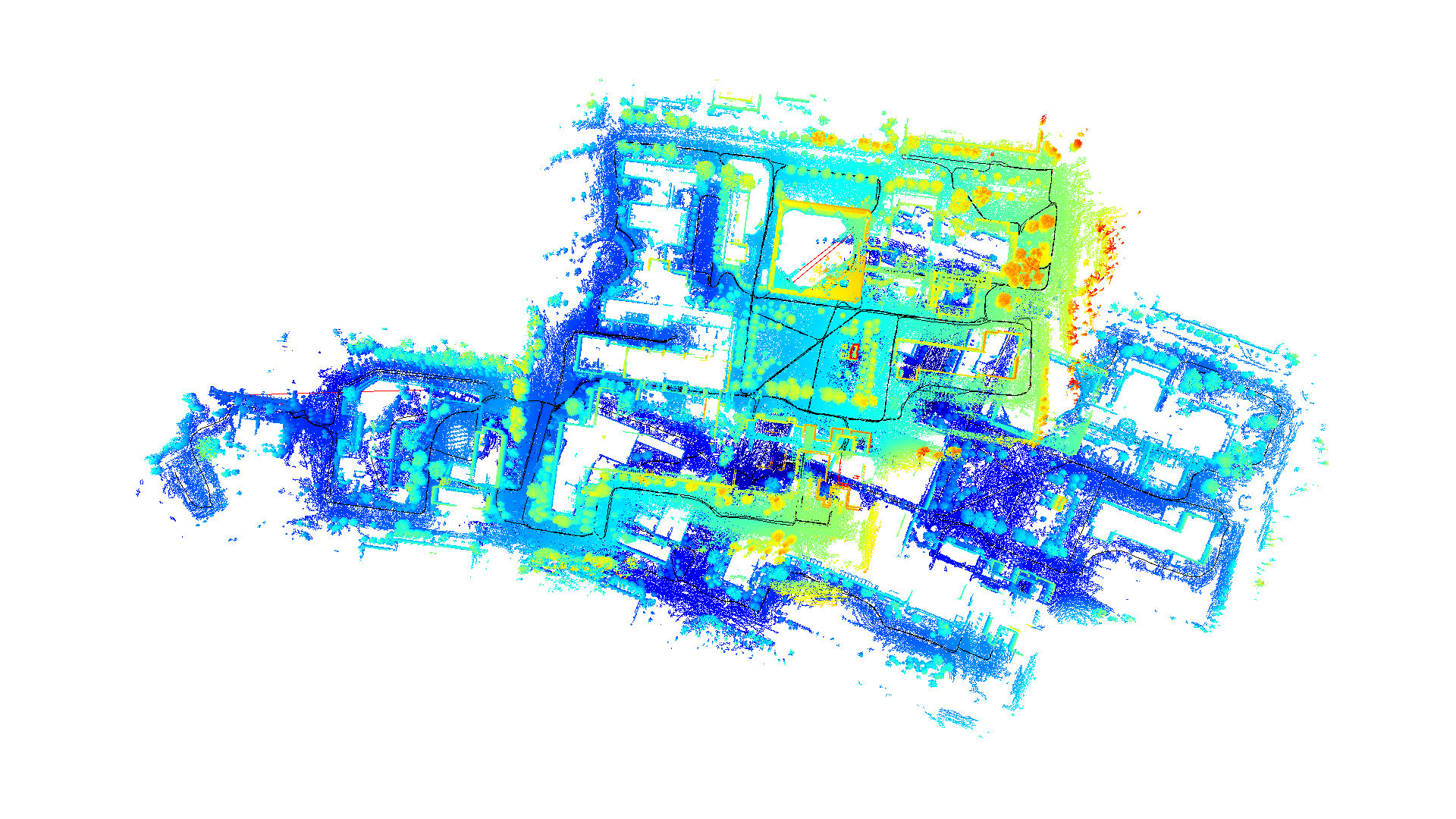
(a) Naïve Method.

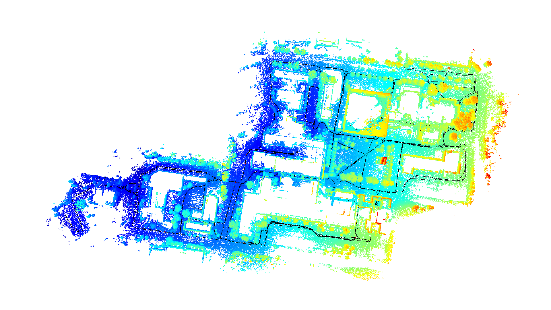
(b) MAC (Nearest).

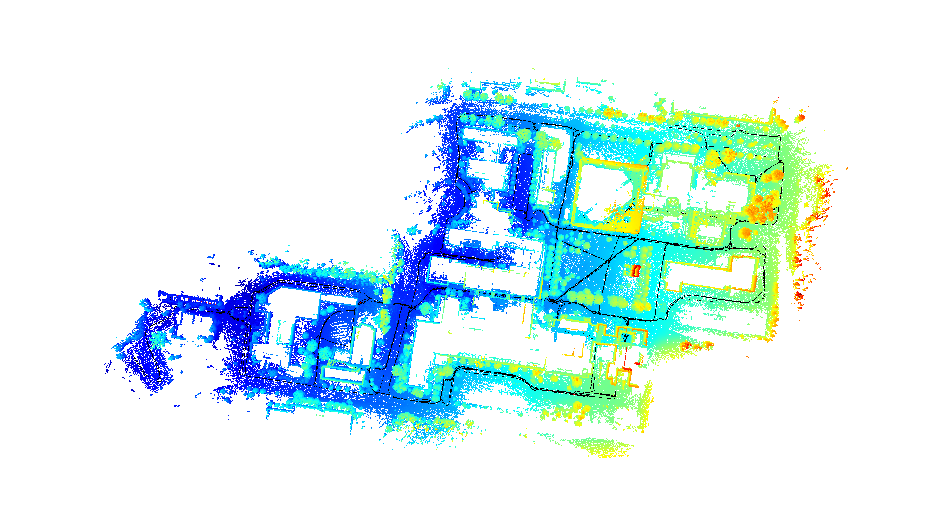
(c) MAC (Madow).

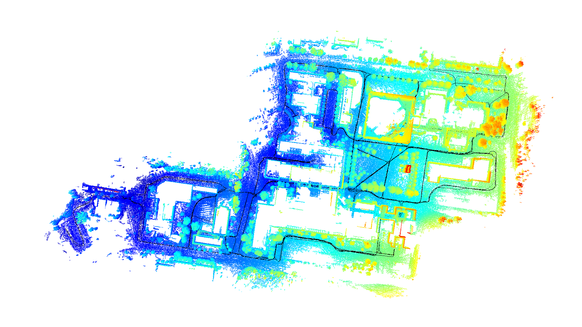
(d) Greedy ESP [20].

Figure 4: Point cloud reconstructions results for the NCLT Dataset. Top-down view of the LiDAR point clouds obtained from SLAM solutions computed using graphs sparsified by each approach to 20% of the total loop closures in the dataset. Point clouds are colored by height in the $z$-axis from blue to red.

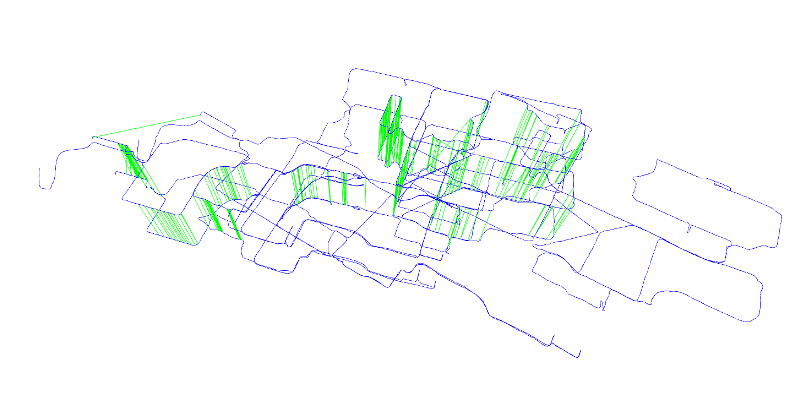
(a) Naïve Method.

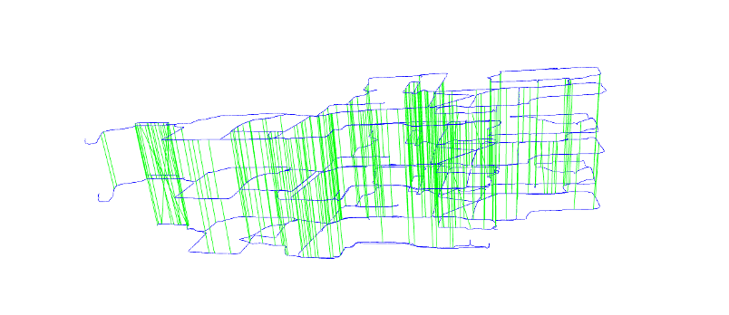
(b) MAC (Madow).

Figure 5: Qualitative results. Offset trajectory visualization comparing the results of the naïve baseline approach with MAC (Madow). Separate trajectories are distributed on the $z$-axis and ordered temporally (i.e. with the trajectory from the first session being the lowest and proceeding upward). Odometry edges are displayed in blue, while loop closures are shown in green. Different viewpoints are used to highlight the impact of poor connectivity in the case of the naïve method. While the first and second sessions are relatively well-connected throughout, the third session is poorly anchored relative to the first two. In contrast, the solution obtained by MAC (Madow) results in a qualitatively more even distribution of loop closure edges throughout, and in turn a higher-quality SLAM solution.

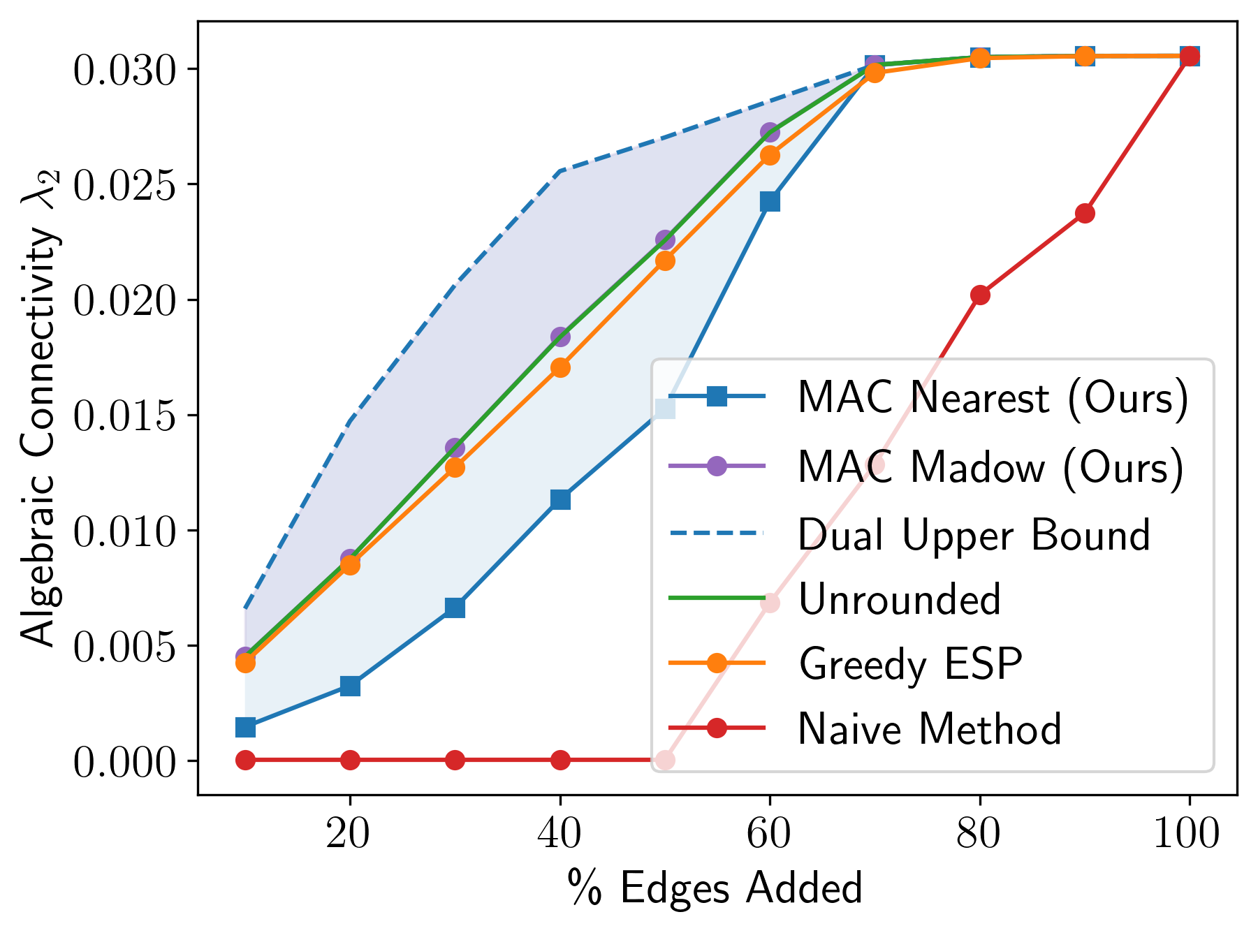
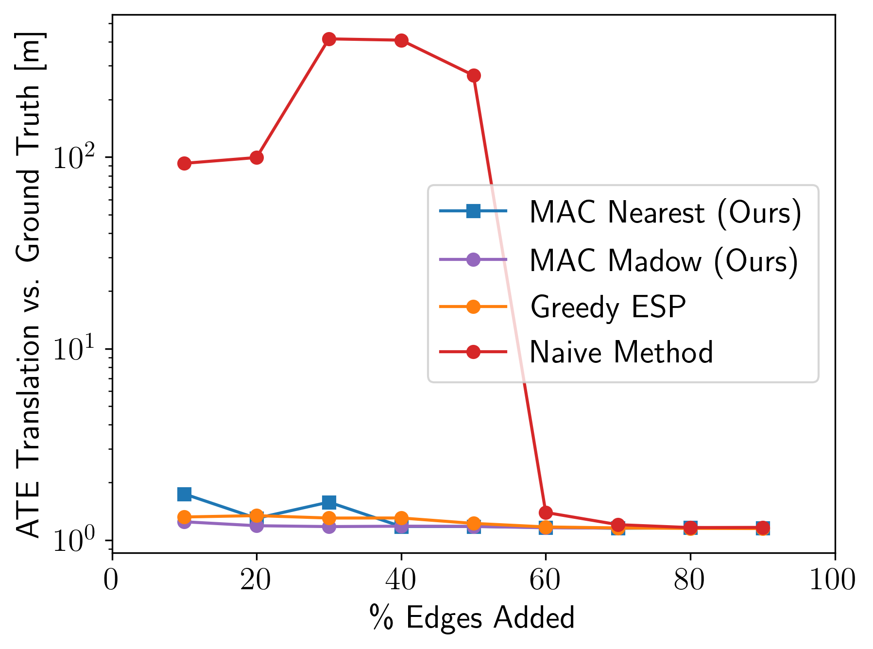
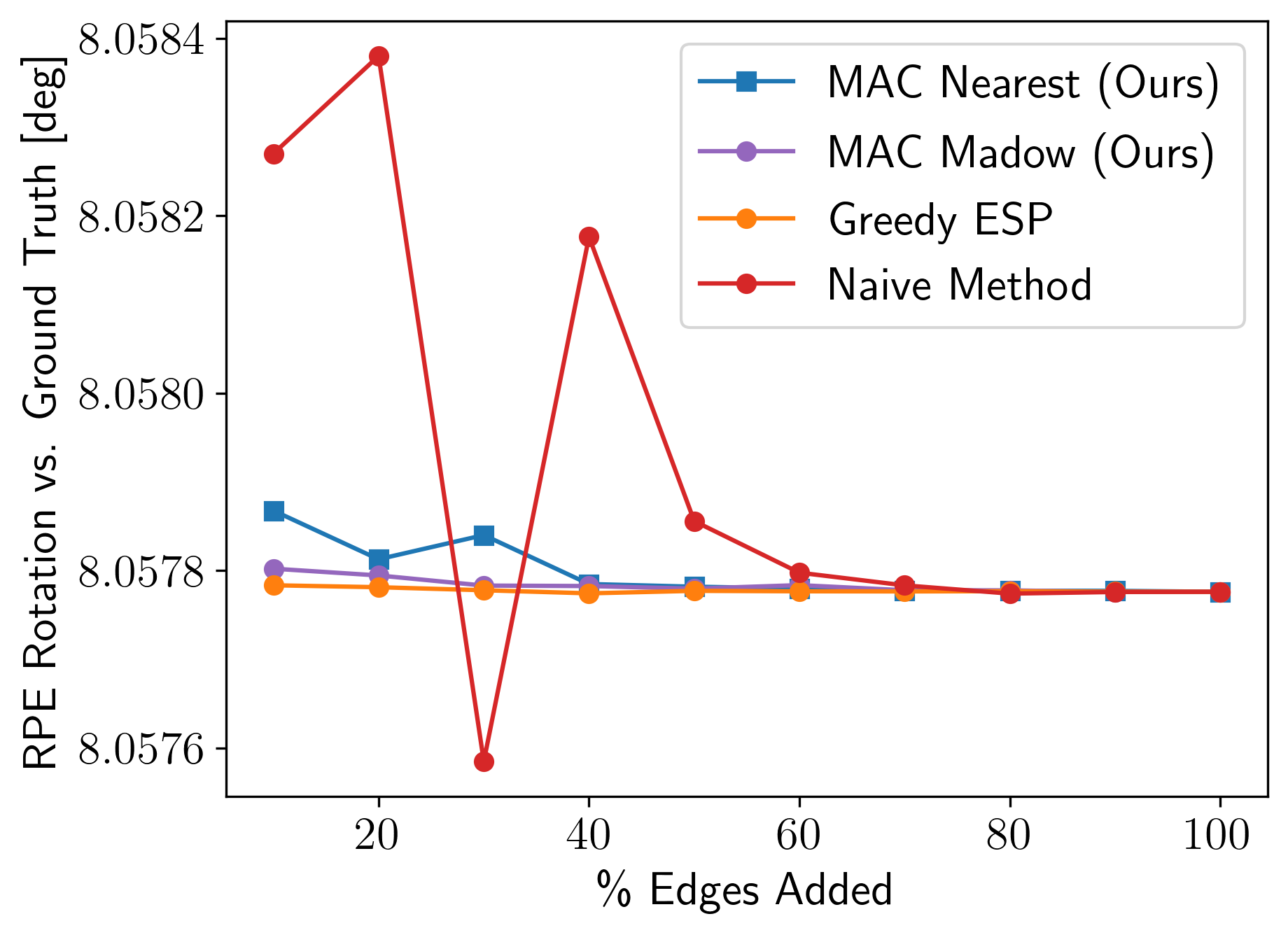
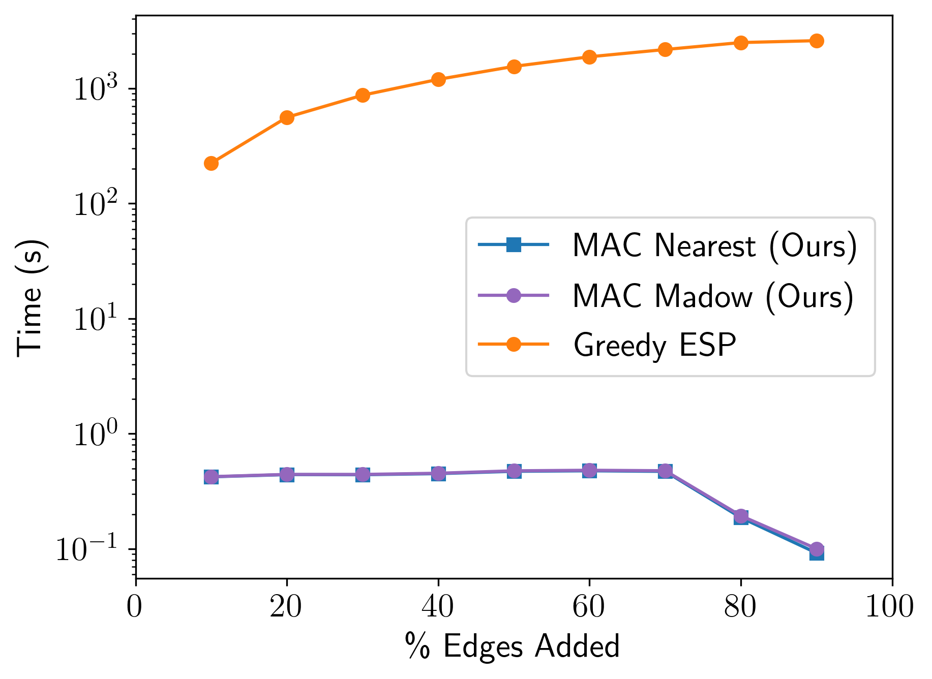
Figure 6: Quantitative results for the NCLT Dataset. Pose-graph optimization results for the NCLT dataset with varying degrees of sparsity (as percent of candidate edges added). Left to right: The algebraic connectivity of the graphs obtained using each method (larger is better) with the shaded regions indicating the suboptimality gap for each MAC rounding procedure, the mean translation error and relative rotation error compared to the ground truth (smaller is better; note that a logarithmic scale used for translation errors, but a linear scale is used for rotation errors), and the computation time (logarithmic scale) for each approach. For 100% loop closures, both algorithms return immediately, so no computation time is reported.

VI Conclusion and Future Work

In this paper, we proposed an approach for graph sparsification by maximizing algebraic connectivity, an important quantity appearing in many applications related to graphs. In particular, the algebraic connectivity has been shown to control the estimation error of pose-graph SLAM solutions, which motivates the application of our algorithm to the setting of pose graph sparsification. Our algorithm, MAC, is based on a first-order optimization approach for solving a convex relaxation of the maximum algebraic connectivity augmentation problem. The algorithm itself is simple and computationally inexpensive, and, as we showed, admits formal post hoc performance guarantees on the quality of the solutions it provides. In experiments on several benchmark pose-graph SLAM datasets, our approach quickly produces high-quality sparsification results which better preserve the connectivity of the graph and, consequently, the quality of SLAM solutions computed using those graphs.

There are many exciting directions for future work on problems related to graph design, algebraic connectivity, and applications to SLAM (or robotics more broadly). From a mathematical standpoint, many practical questions about the relationship between the algebraic connectivity maximization problem 2 and its relaxation 10 remain. For example, in several of the cases we observed, we were able to achieve solutions that appear to be globally optimal with respect to the algebraic connectivity. When this occurred, it was always in the regime where the number of edges to select was relatively large. This was also only the case for a few datasets. It would be interesting to know what properties of the graph under consideration are related, in some sense, to the apparent “difficulty” of solving the algebraic connectivity maximization problem by way of its relaxation in Problem 10. If it is the case that solving problems where more edges are allowed is somehow “easier,” could any performance benefit be gained by solving a sequence of relaxations with increasingly restrictive values of $K$? For example, would this help us find better solutions in the case of smaller $K$, where we generally did not achieve verifiable global optimality in the relaxation (or do so more quickly)?

It would also be useful to have a better understanding of the error introduced during the rounding procedure. As we observed, the introduction of Madow’s systematic sampling method for rounding dramatically improved the quality of our results in some cases. Is there anything we can say, formally, about the error introduced by different rounding methods (or, for example, whether an alternative rounding procedure might be preferred)?

The use of a randomized rounding procedure motivates some interesting additional considerations. For example, by iterating random rounding for a solution $x$ which assigns nonzero probability to every possible $K$-sparse assignment $\hat{x}$, one is guaranteed to eventually obtain a globally optimal solution to Problem 2. This provides an alternative perspective on the goal of the relaxation: namely, to provide a sampling distribution which assigns high probability to globally optimal solutions for Problem 2.

Given that our relaxation allows us to quickly compute approximate solutions (and bounds on solution quality) for large problems, another potential area for future research would be the use of MAC in conjunction with a combinatorial search strategy (e.g. branch-and-bound) or a mixed-integer optimization approach (e.g. as in [26, 27]). In this setting, MAC may be able to accelerate optimization by quickly computing (potentially coarse) bounds on solution quality while retaining the global optimality properties of a combinatorial method.

From an applications standpoint, we have given no suggestion in this paper about how to select an edge budget $K$. We concede that the selection of a value of $K$ will be highly dependent on the application setting of interest. For example, Lajoie and Beltrame [17] determine their edge budget in Swarm-SLAM based on communication constraints. In some cases, it may be desirable to dispose entirely of a hard edge budget constraint, in favor of some smoother regularization. Nam et al. [19] provide an extension of MAC to this setting by regularizing based on the spectrum of the adjacency matrix, but in order for the regularization parameter (trading off solution connectivity for sparsity) to be interpretable, the eigenvalues of the Laplacian and adjacency matrix appearing in their objective must be scaled by the same eigenvalues for the full graph. In applications where the full graph is dense, this computation may be expensive. Moreover, the nonlinearity of the Laplacian spectrum makes it difficult to set a value for that regularization parameter which generalizes across datasets.

Another formulation worth future investigation, inspired by the work of Khosoussi et al. [20], would be to consider moving the algebraic connectivity from the objective to a constraint:

$$\begin{gathered}\min_{x\in\{0,1\}^{m}}\sum_{k=1}^{m}x_{k}\\ \lambda_{2}(x)\geq\delta,\end{gathered}$$ (26)

where $\delta$ is a parameter to be specified by a user. These kinds of spectrally constrained optimization problems were recently considered by Garner et al. [51], who give some potential solution methods for general problems of this form, making it potentially a very fruitful starting point for addressing this variant of the problem. Similar to [19], interpreting $\delta$ requires scaling the problem (for example, we could treat $\delta$ as a fraction of the algebraic connectivity for the graph obtained by keeping all the edges). It would be helpful to come up with an interpretable alternative of the problem in equation (26) that does not require computations related to the full (potentially dense) graph.

There are a number of straightforward variants of Problem 2 that would lend themselves to useful applications. For example, while we consider uniform costs for each edge, it would not be difficult to consider edges having different (appropriately normalized) costs. This would be useful in cases where $K$ corresponds to a communication budget and different amounts of data are required to transmit information about different edges, such as in multi-robot SLAM. Similarly motivated by multi-robot SLAM applications, it is often the case that transmission of a single piece of data is enough to establish more than one edge. This can occur when a single keyframe from one robot can “close the loop” against multiple keyframes from another robot (or vice versa). By attaching a single selection variable $x_{k}$ to a collection of edges that one would obtain by sharing some data, the MAC algorithm can be applied without modification to this setting of “coupled” edges.

The computational performance of MAC motivates its potential application to incremental sparsification. That is, where graph edges are accumulated dynamically over time and sparsification must be performed to ensure bounded computation time and memory requirements. The design of incremental sparsification methods necessarily introduces several new performance considerations above and beyond a single edge budget parameter $K$. One might desire a fixed edge budget, or allow for the number of edges in the graph to grow at a prescribed rate (perhaps as a function of the number of nodes). The application of MAC to the incremental setting is also largely unchanged from its statement in Algorithm 2: we may simply run the “batch” version of MAC to sparsify the graph periodically as new nodes and edges are added. Consequently, while the MAC software library implements some rudimentary examples of incremental sparsification, we do not discuss this setting in our paper. Nonetheless, this is an exciting area for future applications of MAC.

Finally, in this work we consider only the removal of measurement graph edges. For applications like long-term SLAM, an important aspect of future work will be to combine these procedures with methods for node removal (e.g. [4, 2, 52]). An exciting line of inquiry in this direction will be whether methods can be developed for node sparsification (or sparsifying nodes and edges) that preserve some guarantees on graph quality (and, in turn, SLAM quality). Loukas [53] presents some methods that may serve as starting points in this direction.

Appendix A Proofs of the Main Theorems

A-A Supergradients of the Fiedler value

In this subsection we prove Theorem 2, which provides a simple formula for a supergradient of $f(x)=\lambda_{2}(L(x))$.

Our proof is based upon a characterization of the subdifferential of a sum of maximal eigenvalues due to Overton and Womersley [54], which we now briefly recall. Let $\lambda\colon\operatorname{\mathbb{S}}^{n}\to\mathbb{R}^{n}$ be the mapping that assigns to each symmetric matrix $X$ its vector of eigenvalues, counted with multiplicity and sorted in nondecreasing order:

$$\lambda_{1}(X)\leq\dotsb\leq\lambda_{n}(X).$$ (27)

Similarly, given $\kappa\in[n]$, we write $\sigma_{\kappa}\colon\operatorname{\mathbb{S}}^{n}\to\mathbb{R}$ for the (convex) function that assigns to each symmetric matrix $X$ the sum of its $\kappa$ largest eigenvalues:

$$\sigma_{\kappa}(X)\triangleq\sum_{i=1}^{\kappa}\lambda_{n-i+1}(X).$$ (28)

Finally, for $d\geq 1$ and $0\leq\tau\leq d$, define the set:

$$\Phi_{d,\tau}\triangleq\left\{U\in\operatorname{\mathbb{S}}^{d}\mid 0\preceq U\preceq I,\>\operatorname{tr}(U)=\tau\right\}.$$ (29)

Theorem 4 (Theorem 3.5 of [54]).

Let $X\in\operatorname{\mathbb{S}}^{n}$ and

$$X=Q\operatorname{Diag}(\lambda)Q^{\mathsf{T}}$$ (30)

be a symmetric eigendecomposition of $X$. Fix $\kappa\in[n]$, and suppose that $X$’s eigenvalues $\lambda\triangleq\lambda(X)$ satisfy:

$$\lambda_{n}\geq\dotsb\geq\lambda_{n-r+1}\\ >\lambda_{n-r}=\dotsb=\lambda_{n-\kappa+1}=\dotsb=\lambda_{n-(r+t)+1}\\ >\lambda_{n-(r+t)+2}\geq\dotsb\geq\lambda_{1};$$ (31)

that is, there are $r$ eigenvalues strictly greater than the $\kappa$th-largest eigenvalue $\lambda_{n-\kappa+1}$, and $\lambda_{n-\kappa+1}$ has multiplicity $t$. Finally, let $Q_{l}\in\mathbb{R}^{n\times r}$ denote the final $r$ columns of $Q$ (i.e. the eigenvectors associated with the top $r$-dimensional invariant subspace of $X$), and $Q_{p}$ the preceding block of $t$ columns (i.e. the set of $t$ eigenvectors associated with the $\kappa$th eigenvalue $\lambda_{n-\kappa+1}$). Then the subdifferential of $\sigma_{\kappa}$ at $X$ is:

$$\partial\sigma_{\kappa}(X)=\left\{Q_{l}Q_{l}^{\mathsf{T}}+Q_{p}UQ_{p}^{\mathsf{T}}\mid U\in\Phi_{t,\kappa-r}\right\}.$$ (32)

Proof of Theorem 2.

Let

$$\begin{gathered}\eta\colon[0,1]^{m}\to\mathbb{R}\\ \eta(x)\triangleq\sigma_{2}(-L(x))\end{gathered}$$ (33)

where $L\colon[0,1]^{m}\to\mathbb{S}_{+}^{n}$ is the PSD-matrix-valued affine map defined in (8). Then

$$\eta(x)=-\lambda_{1}(L(x))-\lambda_{2}(L(x))=-\lambda_{2}(L(x))$$ (34)

since $\lambda_{1}(L(x))=0$ as $L(x)$ is a graph Laplacian. Note that (34) implies $f(x)=\lambda_{2}(L(x))$ is concave, since $\eta(x)=-f(x)$ is convex. Moreover, since the domain of $\sigma_{2}(x)$ is all of $\mathbb{R}^{n}$ and $L(x)$ is smooth, the subdifferential chain rule (cf. Example 7.27 and Theorem 10.6 of [55]) implies:

$$\partial\eta(x)=\left\{-\nabla L(x)^{*}[W]\mid W\in\partial\sigma_{2}(-L(x))\right\},$$ (35)

where ^∗ denotes the adjoint.

Now let $q_{2}\in\mathbb{R}^{n}$ be any normalized eigenvector of $\lambda_{2}(L(x))$ that is orthogonal to $\mathbbm{1}$. Since

$$\lambda_{n-i+1}(-L(x))=-\lambda_{i}(L(x))\quad\quad\forall i\in[n]$$ (36)

and $\mathbbm{1}$ is an eigenvector of $\lambda_{1}(L(x))=0$, we may factor $-L(x)$ as:

$$-L(x)=Q\operatorname{Diag}\left[\lambda(-L(x))\right]Q^{\mathsf{T}},$$ (37)

where $Q$ has the form:

$$Q=\begin{pmatrix}P&q_{2}&\frac{1}{\sqrt{n}}\mathbbm{1}\end{pmatrix}\in\operatorname{O}(n).$$ (38)

We claim that:

$$V\triangleq\frac{1}{n}\mathbbm{1}\mathbbm{1}^{\mathsf{T}}+q_{2}q_{2}^{\mathsf{T}}\in\partial\sigma_{2}(-L(x)).$$ (39)

To prove this, we will consider two cases.

Case 1: $\lambda_{2}(L(x))>0$. Since $\lambda_{1}(L(x))=0$ (as $L(x)$ is a graph Laplacian), equation (36) shows that the maximum eigenvalue of $-L(x)$ is simple. Consequently, applying Theorem 4 with factorization (37)–(38) (and $r=1$), we find that:

$$\partial\sigma_{2}(-L(x))=\left\{\frac{1}{n}\mathbbm{1}\mathbbm{1}^{\mathsf{T}}+Q_{p}UQ_{p}^{\mathsf{T}}\mid U\in\Phi_{t,1}\right\}.$$ (40)

In particular, taking

$$U=\begin{pmatrix}0_{(t-1)\times(t-1)}&\\ &1\end{pmatrix}\in\Phi_{t,1}$$ (41)

in (40) and recalling (38) establishes (39).

Case 2: $\lambda_{2}(L(x))=0$. In this case $\lambda_{1}(L(x))=\lambda_{2}(L(x))=0$. Consequently, applying Theorem 4 with factorization (37)–(38) (and $r=0$), we find that:

$$\partial\sigma_{2}(-L(x))=\left\{Q_{p}UQ_{p}^{\mathsf{T}}\mid U\in\Phi_{t,2}\right\}.$$ (42)

In particular, taking

$$U=\begin{pmatrix}0_{(t-2)\times(t-2)}&\\ &I_{2}\end{pmatrix}\in\Phi_{t,2}$$ (43)

in (42) and recalling (38) establishes (39).

Equations (35) and (39) together imply that:

$$y\triangleq-\nabla L(x)^{*}[V]\in\partial\eta(x).$$ (44)

Moreover, it follows from (8) that the elements of $y$ are given explicitly by:

$$\begin{split}y_{k}&=\left\langle-L^{c}_{k},\>\frac{1}{n}\mathbbm{1}\mathbbm{1}^{\mathsf{T}}+q_{2}q_{2}^{\mathsf{T}}\right\rangle\\ &=-\frac{1}{n}\mathbbm{1}^{\mathsf{T}}L^{c}_{k}\mathbbm{1}-q_{2}^{\mathsf{T}}L^{c}_{k}q_{2}\\ &=-q_{2}^{\mathsf{T}}L^{c}_{k}q_{2},\end{split}$$ (45)

since $\mathbbm{1}\in\ker(L^{c}_{k})$ for all $k$. Comparing (45) and (12) shows that $y=-g$, and thus $-g\in\partial\eta(x)$. Finally, recalling that $\eta(x)=-\lambda_{2}(L(x))$ [cf. (34)] shows that $g$ as defined in (12) is a supergradient of $\lambda_{2}(L(x))$, as claimed. ∎

A-B Solving the direction-finding subproblem (Problem 4)

This appendix aims to prove the claim that (14) provides an optimal solution to the linear program in Problem 4.

Proof of Theorem 3.

Rewriting the objective from Problem 4 in terms of the elements of $s$ and $g(x)$, we have:

$$g^{\mathsf{T}}s =\sum_{k=1}^{m}g_{k}s_{k},$$ (46)

$$=\sum_{k=1}^{m}s_{k}q_{2}^{\mathsf{T}}L^{c}_{k}q_{2},$$

where in the last line we have used the definition of $g_{k}$ in (12). Now, since the component-wise Laplacian matrices $L^{c}_{k}\succeq 0$ for each edge $k$, every component of the supergradient must always be nonnegative, i.e. $g_{k}\geq 0$. Further, since $0\leq s_{k}\leq 1$, the objective in (46) is itself a sum of nonnegative terms. From this, it follows directly that the objective in (46) is maximized (subject to the constraint that $\sum_{k=1}^{m}s_{k}=K$) specifically by selecting (i.e., by setting $s_{k}=1$) each of the $K$ largest components of $g(x)$, giving the result in (14). ∎

References

- Rosen et al. [2021] D. M. Rosen, K. J. Doherty, A. T. Espinoza, and J. J. Leonard, “Advances in Inference and Representation for Simultaneous Localization and Mapping,” Annual Review of Control, Robotics, and Autonomous Systems, vol. 4, no. 1, pp. 215–242, 2021. [Online]. Available: https://doi.org/10.1146/annurev-control-072720-082553
- Carlevaris-Bianco and Eustice [2013] N. Carlevaris-Bianco and R. M. Eustice, “Long-term simultaneous localization and mapping with generic linear constraint node removal,” in IEEE/RSJ Intl. Conf. on Intelligent Robots and Systems (IROS), Tokyo, Japan, Nov. 2013.
- Carlevaris-Bianco and Eustice [2014] ——, “Conservative edge sparsification for graph SLAM node removal,” in 2014 IEEE International Conference on Robotics and Automation (ICRA). IEEE, 2014, pp. 854–860.
- Johannsson et al. [2012] H. Johannsson, M. Kaess, M. Fallon, and J. Leonard, “Temporally scalable visual SLAM using a reduced pose graph,” in RSS Workshop on Long-term Operation of Autonomous Robotic Systems in Changing Environments, Sydney, Australia, Jul. 2012, available as MIT CSAIL Technical Report MIT-CSAIL-TR-2012-013.
- Kurz et al. [2021] G. Kurz, M. Holoch, and P. Biber, “Geometry-based graph pruning for lifelong SLAM,” arXiv preprint arXiv:2110.01286, 2021.
- Kretzschmar and Stachniss [2012] H. Kretzschmar and C. Stachniss, “Information-theoretic compression of pose graphs for laser-based SLAM,” The International Journal of Robotics Research, vol. 31, no. 11, pp. 1219–1230, 2012.
- Boumal et al. [2014] N. Boumal, A. Singer, P.-A. Absil, and V. D. Blondel, “Cramér–Rao bounds for synchronization of rotations,” Information and Inference: A Journal of the IMA, vol. 3, no. 1, pp. 1–39, 2014.
- Chen et al. [2021] Y. Chen, S. Huang, L. Zhao, and G. Dissanayake, “Cramér–Rao bounds and optimal design metrics for pose-graph SLAM,” IEEE Transactions on Robotics, vol. 37, no. 2, pp. 627–641, 2021.
- Khosoussi et al. [2014] K. Khosoussi, S. Huang, and G. Dissanayake, “Novel insights into the impact of graph structure on SLAM,” in 2014 IEEE/RSJ International Conference on Intelligent Robots and Systems. IEEE, 2014, pp. 2707–2714.
- Rosen et al. [2019] D. M. Rosen, L. Carlone, A. S. Bandeira, and J. J. Leonard, “SE-Sync: A certifiably correct algorithm for synchronization over the special Euclidean group,” Intl. J. of Robotics Research, vol. 38, no. 2-3, pp. 95–125, 2019.
- Doherty et al. [2022a] K. J. Doherty, D. M. Rosen, and J. J. Leonard, “Performance Guarantees for Spectral Initialization in Rotation Averaging and Pose-Graph SLAM,” in IEEE Intl. Conf. on Robotics and Automation (ICRA), 2022.
- Spielman and Teng [2011] D. A. Spielman and S.-H. Teng, “Spectral sparsification of graphs,” SIAM Journal on Computing, vol. 40, no. 4, pp. 981–1025, 2011.
- Pukelsheim [2006] F. Pukelsheim, Optimal design of experiments. SIAM, 2006.
- Mosk-Aoyama [2008] D. Mosk-Aoyama, “Maximum algebraic connectivity augmentation is NP-hard,” Operations Research Letters, vol. 36, no. 6, pp. 677–679, 2008.
- Ghosh and Boyd [2006] A. Ghosh and S. Boyd, “Growing well-connected graphs,” in Proceedings of the 45th IEEE Conference on Decision and Control. IEEE, 2006, pp. 6605–6611.
- Doherty et al. [2022b] K. J. Doherty, D. M. Rosen, and J. J. Leonard, “Spectral Measurement Sparsification for Pose-Graph SLAM,” in IEEE/RSJ Intl. Conf. on Intelligent Robots and Systems (IROS), 2022.
- Lajoie and Beltrame [2024] P.-Y. Lajoie and G. Beltrame, “Swarm-SLAM: Sparse decentralized collaborative simultaneous localization and mapping framework for multi-robot systems,” IEEE Robotics and Automation Letters, vol. 9, no. 1, pp. 475–482, 2024.
- Kaveti et al. [2023] P. Kaveti, M. Giamou, H. Singh, and D. M. Rosen, “OASIS: Optimal Arrangements for Sensing in SLAM,” arXiv preprint arXiv:2309.10698, 2023.
- Nam et al. [2023] J. Nam, S. Hyeon, Y. Joo, D. Noh, and H. Shim, “Spectral trade-off for measurement sparsification of pose-graph SLAM,” IEEE Robotics and Automation Letters, vol. 9, no. 1, pp. 723–730, 2023.
- Khosoussi et al. [2019] K. Khosoussi, M. Giamou, G. S. Sukhatme, S. Huang, G. Dissanayake, and J. P. How, “Reliable graphs for SLAM,” The International Journal of Robotics Research, vol. 38, no. 2-3, pp. 260–298, 2019.
- Boyd [2006] S. Boyd, “Convex optimization of graph Laplacian eigenvalues,” in Proceedings of the International Congress of Mathematicians, vol. 3, no. 1-3. Citeseer, 2006, pp. 1311–1319.
- Fiedler [1973] M. Fiedler, “Algebraic connectivity of graphs,” Czechoslovak mathematical journal, vol. 23, no. 2, pp. 298–305, 1973.
- Lewis and Overton [1996] A. S. Lewis and M. L. Overton, “Eigenvalue optimization,” Acta numerica, vol. 5, pp. 149–190, 1996.
- Lewis [2003] A. S. Lewis, “The mathematics of eigenvalue optimization,” Mathematical Programming, vol. 97, no. 1, pp. 155–176, 2003.
- Shapiro and Fan [1995] A. Shapiro and M. K. Fan, “On eigenvalue optimization,” SIAM Journal on Optimization, vol. 5, no. 3, pp. 552–569, 1995.
- Nagarajan [2018] H. Nagarajan, “On maximizing weighted algebraic connectivity for synthesizing robust networks,” arXiv preprint arXiv:1805.07825, 2018.
- Somisetty et al. [2023] N. Somisetty, H. Nagarajan, and S. Darbha, “Optimal robust network design: Formulations and algorithms for maximizing algebraic connectivity,” arXiv preprint:2304.08571, 2023. [Online]. Available: https://arxiv.org/abs/2304.08571
- Huang et al. [2013] G. Huang, M. Kaess, and J. Leonard, “Consistent sparsification for graph optimization,” in Proc. of European Conference on Mobile Robots (ECMR), Barcelona, Spain, Sep. 25–27, 2013, pp. 150–157.
- Tian and How [2023] Y. Tian and J. P. How, “Spectral sparsification for communication-efficient collaborative rotation and translation estimation,” IEEE Trans. Robotics, 2023.
- Kim and Eustice [2009] A. Kim and R. Eustice, “Toward AUV survey design for optimal coverage and localization using the Cramer Rao lower bound,” in Proc. of the IEEE/MTS OCEANS Conf. and Exhibition, 2009.
- Papalia et al. [2022] A. Papalia, N. Thumma, and J. Leonard, “Prioritized planning for cooperative range-only localization in multi-robot networks,” in 2022 International Conference on Robotics and Automation (ICRA). IEEE, 2022, pp. 10 753–10 759.
- Mesbahi and Egerstedt [2010] M. Mesbahi and M. Egerstedt, Graph Theoretic Methods in Multiagent Networks. Princeton University Press, 2010.
- Boyd and Vandenberghe [2004] S. Boyd and L. Vandenberghe, Convex Optimization. Cambridge University Press, 2004.
- Rockafellar [2015] R. T. Rockafellar, Convex analysis. Princeton university press, 2015.
- Dellaert et al. [2020] F. Dellaert, D. M. Rosen, J. Wu, R. Mahony, and L. Carlone, “Shonan rotation averaging: Global optimality by surfing SO(p),” in European Conference on Computer Vision. Springer, 2020, pp. 292–308.
- Bertsekas [2016] D. Bertsekas, Nonlinear Programming. Athena Scientific, 2016, vol. 4.
- Dunn and Harshbarger [1978] J. C. Dunn and S. Harshbarger, “Conditional gradient algorithms with open loop step size rules,” Journal of Mathematical Analysis and Applications, vol. 62, no. 2, pp. 432–444, 1978.
- Manguoglu et al. [2010] M. Manguoglu, E. Cox, F. Saied, and A. Sameh, “TRACEMIN-Fiedler: A parallel algorithm for computing the Fiedler vector,” in International Conference on High Performance Computing for Computational Science. Springer, 2010, pp. 449–455.
- Sameh and Wisniewski [1982] A. H. Sameh and J. A. Wisniewski, “A trace minimization algorithm for the generalized eigenvalue problem,” SIAM Journal on Numerical Analysis, vol. 19, no. 6, pp. 1243–1259, 1982.
- Madow [1949] W. G. Madow, “On the Theory of Systematic Sampling, II,” The Annals of Mathematical Statistics, vol. 20, no. 3, pp. 333–354, 1949.
- Paria and Sinha [2021] D. Paria and A. Sinha, “LeadCache: Regret-Optimal Caching in Networks,” Advances in Neural Information Processing Systems, vol. 34, pp. 4435–4447, 2021.
- Lacoste-Julien et al. [2013] S. Lacoste-Julien, M. Jaggi, M. Schmidt, and P. Pletscher, “Block-coordinate frank-wolfe optimization for structural svms,” in International Conference on Machine Learning. PMLR, 2013, pp. 53–61.
- Chen et al. [2008] Y. Chen, T. A. Davis, W. W. Hager, and S. Rajamanickam, “Algorithm 887: Cholmod, supernodal sparse cholesky factorization and update/downdate,” ACM Trans. Math. Softw., vol. 35, no. 3, oct 2008. [Online]. Available: https://doi.org/10.1145/1391989.1391995
- Carlevaris-Bianco et al. [2015] N. Carlevaris-Bianco, A. K. Ushani, and R. M. Eustice, “University of Michigan North Campus long-term vision and lidar dataset,” International Journal of Robotics Research, vol. 35, no. 9, pp. 1023–1035, 2015.
- Krause and Golovin [2014] A. Krause and D. Golovin, “Submodular function maximization,” Tractability, vol. 3, no. 71-104, p. 3, 2014.
- Minoux [2005] M. Minoux, “Accelerated greedy algorithms for maximizing submodular set functions,” in Optimization Techniques: Proceedings of the 8th IFIP Conference on Optimization Techniques Würzburg, September 5–9, 1977. Springer, 2005, pp. 234–243.
- Xu et al. [2022] W. Xu, Y. Cai, D. He, J. Lin, and F. Zhang, “Fast-LIO2: Fast direct lidar-inertial odometry,” IEEE Trans. Robotics, vol. 38, no. 4, pp. 2053–2073, 2022.
- Kim and Kim [2018] G. Kim and A. Kim, “Scan context: Egocentric spatial descriptor for place recognition within 3d point cloud map,” in IEEE/RSJ Intl. Conf. on Intelligent Robots and Systems (IROS). IEEE, 2018, pp. 4802–4809.
- Huang et al. [2021] Y. Huang, T. Shan, F. Chen, and B. Englot, “DiSCo-SLAM: Distributed scan context-enabled multi-robot lidar SLAM with two-stage global-local graph optimization,” IEEE Robotics and Automation Letters, vol. 7, no. 2, pp. 1150–1157, 2021.
- Dellaert [2012] F. Dellaert, “Factor graphs and GTSAM: A hands-on introduction,” Georgia Institute of Technology, Tech. Rep., 2012.
- Garner et al. [2023] C. Garner, G. Lerman, and S. Zhang, “Spectrally Constrained Optimization,” arXiv preprint arXiv:2307.04069, 2023.
- Carlone et al. [2014] L. Carlone, Z. Kira, C. Beall, V. Indelman, and F. Dellaert, “Eliminating conditionally independent sets in factor graphs: A unifying perspective based on smart factors,” in Robotics and Automation (ICRA), 2014 IEEE International Conference on. IEEE, 2014, pp. 4290–4297.
- Loukas [2019] A. Loukas, “Graph reduction with spectral and cut guarantees.” J. Mach. Learn. Res., vol. 20, no. 116, pp. 1–42, 2019.
- Overton and Womersley [1993] M. L. Overton and R. S. Womersley, “Optimality conditions and duality theory for minimizing sums of the largest eigenvalues of symmetric matrices,” Mathematical Programming, vol. 62, no. 1, pp. 321–357, 1993.
- Rockafellar and Wets [2009] R. Rockafellar and R.-B. Wets, Variational Analysis. Springer Science+Business Media, 2009.