Re-thinking Uncertainty Quantification Metrics for Semantic Segmentation

Abstract

Keywords Semantic Segmentation  $\cdot$ Uncertainty Quantification  $\cdot$ PAvPU

In the domain of computer vision, semantic segmentation emerges as a fundamental application within machine learning, wherein individual pixels of an image are classified into distinct semantic categories. This task transcends traditional accuracy metrics by incorporating uncertainty quantification, a critical measure for assessing the reliability of each segmentation prediction. Such quantification is instrumental in facilitating informed decision-making, particularly in applications where precision is paramount. Within this nuanced framework, the metric known as PAvPU (Patch Accuracy versus Patch Uncertainty) has been developed as a specialized tool for evaluating entropy-based uncertainty in image segmentation tasks. However, our investigation identifies three core deficiencies within the PAvPU framework and proposes robust solutions aimed at refining the metric. By addressing these issues, we aim to enhance the reliability and applicability of uncertainty quantification, especially in scenarios that demand high levels of safety and accuracy, thus contributing to the advancement of semantic segmentation methodologies in critical applications.

1 Introduction

Semantic segmentation, a cornerstone of image processing, plays a pivotal role in critical applications across healthcare and robotics. This process, which categorizes each pixel in an image into specific classes, is fundamental for tasks ranging from tumor detection [1, 2, 3, 4, 5] and organ delineation [6, 7, 8, 9] in medical imaging to enabling nuanced perception [10, 11, 12, 13] and decision-making [13, 14, 15, 16] in autonomous systems. The accuracy of these models, while paramount, is only part of the equation. Equally crucial is the ability to numerically quantify how reliable an individual prediction is [17] — this is where uncertainty quantification (UQ) comes into play. UQ is like the model’s way of saying, "I think this is the answer, but here’s how confident I am about it." It not only enhances the trustworthiness of segmentation models but also provides invaluable insights for clinical decision-making in healthcare [18, 19, 20, 21] and navigational certainty in robotics [22, 23] amidst the myriad of real-world ambiguities.

Despite UQ’s key role across many applications, its tasks in semantic segmentation face multifaceted challenges. The sheer computational complexity is daunting; each pixel’s classification in an H×W image multiplies the scale of predictions, especially in high-resolution images. This complexity is further compounded by the inherent dependencies among neighboring pixels, driven by the spatial correlations within the image’s structural features like edges and textures. Such dependencies necessitate sophisticated UQ methods that consider these spatial relationships. Additionally, the widespread problem of class imbalance, particularly noticeable in autonomous driving, affects the process of assessing prediction certainty. In such scenarios, less frequent elements like pedestrians, bicycles, or rare road signs are overshadowed by more common features like roads, skies, or cars. This imbalance can lead to the system being overly confident in its predictions about the more prevalent classes, while potentially overlooking the less common, yet crucial, ones. Adding to the complexity is the challenge of accurately quantifying uncertainty at object boundaries, where pixel classifications are most prone to ambiguity due to overlapping features or occlusions.

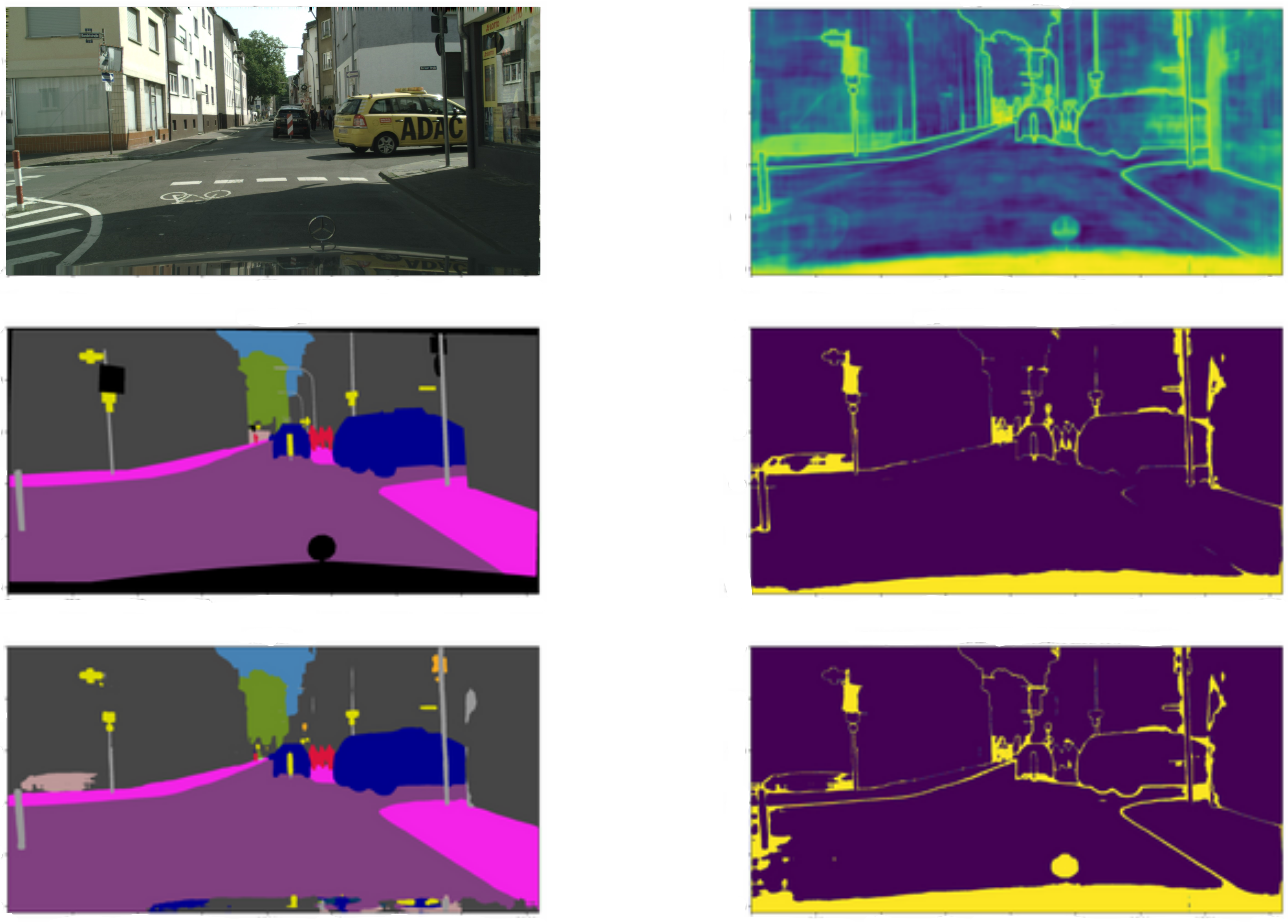
Figure 1: Deeplabv3 + LeftTop: Original Image. LeftMiddle:Ground Truth. LeftBottom: Prediction. RightTop Log Total Uncertainty. RightMiddle: Total Uncertainty   .95 Quantile. RightBottom: Categorical Uncertainty   .95 Categorical Quantile

Figure 1 outlines the challenges at hand. Initially, the photo reveals how obstructions, namely a traffic sign and a building, partially hide the vehicle, creating a complex scene for analysis. This complexity leads to the model’s difficulties in accurately distinguishing the edges of each element, as demonstrated in the lower-left portion of the figure. This issue is further compounded by the uncertainty depicted in the top-right section, which underscores the ambiguities in object boundaries. Notably, this uncertainty is not uniformly distributed but shows a spatial correlation, meaning areas close to one another share similar levels of uncertainty. Another significant challenge highlighted is the issue of class imbalance, with road pixels being overwhelmingly more common. This imbalance influences the uncertainty levels, which are also dependent on the category of the objects, with less common categories exhibiting greater uncertainty. This phenomenon is particularly noticeable in the comparison between the middle-right and bottom-right plots, where the categorical uncertainty helps to delineate the boundaries between objects more clearly, offering deeper insights into the model’s performance and the inherent challenges of the scene.

Given these hurdles and the general absence of ground truth uncertainty for validation, the field often relies on simplified metrics that, while computationally efficient, tend to mix different types of information and struggle to provide fair comparisons across various methods. These metrics frequently depend on indirect measures like accuracy or employ grouping mechanisms that may not fully capture the nuanced interplay of uncertainties among adjacent pixels or the abrupt shifts in uncertainty at boundaries.

Acknowledging these limitations necessitates a nuanced evaluation of the current metrics used for UQ in semantic segmentation. Our work delves into this realm, with a keen focus on the widely utilized Patch Accuracy versus Patch Uncertainty (PAvPU) metric [24]. PAvPU synthesizes accuracy and uncertainty quantification at a patch level, offering a pragmatic balance between computational feasibility and the granularity of uncertainty representation. By aligning patch-level accuracy and uncertainty within a binary threshold framework, PAvPU leverages spatial pixel relationships to mitigate cross-patch dependency issues. Yet, despite its merits, PAvPU is not without its limiations. It can be swayed by the specific settings for patch size and thresholds, requiring precise adjustments. It may also falter in the face of class imbalance, tending to favor more common classes while discriminating critical but less frequent ones. It struggles as well with the fuzziness in object boundary definitions. Most importantly, PAvPU, as with any metric, might not suit every model or situation, necessitating adaptation and perhaps the integration with other metrics to ensure a holistic assessment of a model’s effectiveness.

In light of these considerations, our investigation aims to unravel these complexities, enhancing the utility of PAvPU while addressing its inherent limitations. By incorporating a supplementary metric, we address the limitations tied to PAvPU’s accuracy dependency. This initiative highlights that, under this comprehensive metric system, the issues of patch size and boundary fuzziness are significantly diminished. Furthermore, by reporting the metric at the categorical level, we tackle the problem of class imbalance head-on. This integrated approach effectively bridges these solutions, forging a path toward a refined and reliable framework in uncertainty quantification within semantic segmentation.

2 Background

Uncertainty in ML In the field of machine learning, uncertainty is classified into aleatoric, related to inherent data variability, and epistemic, associated with the model’s limited knowledge [25]. The endeavor of uncertainty disentanglement seeks to differentiate between these sources, determining whether the uncertainty arises from the data’s intrinsic characteristics or from the model’s interpretative limitations. Entropy [26], a notion in information theory, plays a pivotal role in this context by providing a measure of the unpredictability inherent in the model’s predictions. Given a group of candidate models’ output distribution $Q_{i}$ and their average as the ensemble centroid $P=\frac{1}{I}\Sigma_{i}Q_{i}$. The total uncertainty can be decomposed:

$H(P)\text{ ( Total U ) }=\frac{1}{I}\Sigma_{i}D_{KL}(Q_{i}||P)\text{ ( Epistemic U ) }+\frac{1}{I}H(Q_{i})\text{ ( Aleotoric U )}$. $H$ is entropy. $D_{KL}$ is KL divergence.

This incorporation of entropy into the disentanglement process allows for a more sophisticated analysis, facilitating a deeper comprehension of uncertainty’s roots.

Semantic segmentation Semantic segmentation serves the purpose of categorizing each pixel in an image into designated classes, effectively dissecting the image into segments that hold meaningful semantic value. The essence of semantic segmentation lies in its ability to maintain consistency by ensuring that pixels pertaining to the same object are recognized under a unified label. Furthermore, the process is designed to be contextually aware, processing the image in its entirety to ascertain a comprehensive context. Such an approach is instrumental in enabling the algorithm to grasp the intricate interplay between adjacent pixels, thereby facilitating a segmentation that boasts a high degree of precision.

In this research, we utilize models that feature the same encoder configurations for our control tests. This method is chosen due to the greater variability observed in model structures that rely on entropy for uncertainty estimation, in contrast to deterministic models that determine uncertainty through calibration error. DeepLabV3 [27] introduced atrous convolution and Atrous Spatial Pyramid Pooling (ASPP), enhancing contextual details by expanding the receptive fields. DeepLabV3+ [28] further improved feature representation by merging high-level and low-level features. CCNet [29] applied a Criss-Cross Attention mechanism for comprehensive global context through sequential attention across rows and columns. The Asymmetric Non-local Network (ANN) [30] and Adaptive Pyramid Context Network (APCNet) optimized attention targeting and feature integration for computational efficiency, with APCNet [31] focusing on multi-scale attentions. The Dynamic Multi-scale Filters Network (DMNet) [32] incorporated contextual information into its filters, deviating from conventional methods, while the Dual Attention Network (DANet) [33] utilized spatial and channel attentions for improved communication. PSANet[34] introduced a mechanism to enhance spatial awareness by connecting any two points directly. Despite a shared backbone, the unique decoder designs in these models lead to varied handling of feature disruptions, allowing us to explore how different approaches to processing encoder outputs affect uncertainty quantification.

Metrics for uncertainty quantification in semantic segmentation In the realm of machine learning, gauging uncertainty is pivotal for validating the credibility of probabilistic forecasts. We will explore three hallmark metrics, each embodying a critical aspect of uncertainty quantification. PAvPU (Patch Accuracy versus Patch Uncertainty) [24], ECE (Expected Calibration Error) [35], and AUSE (Area Under the Sparsification Error curve) [36]. PAvPU assesses the relationship between the accuracy of predictions and the associated uncertainty at a patch level within an image, providing insight into whether high-confidence predictions correlate with high accuracy and vice versa for low-confidence predictions. This is particularly useful in tasks where local decisions (e.g., in patches of an image) are critical, and understanding the spatial distribution of uncertainty is important. ECE, on the other hand, measures the calibration of a model’s predicted probabilities against the actual outcomes across the entire dataset, offering a global view of how well the predicted uncertainties align with the true error rates. ECE is widely used for classification tasks but can also be adapted for segmentation. AUSE evaluates the performance of uncertainty quantification by measuring the error (e.g., segmentation error) as a function of the amount of data (e.g., pixels or patches) being considered, based on their estimated uncertainty. This metric effectively illustrates how well a model’s uncertainty estimates can identify and discard the most uncertain (and presumably the least accurate) predictions to improve the overall performance.

Among the metrics evaluated, PAvPU distinguishes itself by being the most computationally efficient, requiring neither calibration nor sorting, and it uniquely accommodates entropy-based uncertainty which breaks down total uncertainty into two complementary components. In view of this, our work concentrates on the refinement of PAvPU by introducing an axuliary metric, which uncovers and rectifies PAvPU’s blind spots, paving the way for a more discerning and reliable uncertainty quantification in semantic segmentation.

3 Local Nature of Entropy-Based Uncertainty as the UQ method and PAvPU as the corresponding UQ metric

In the realm of image segmentation, the incorporation of contextual cues is indispensable for the precise classification of individual pixels. While the current trajectory in machine learning, especially within uncertainty quantification (UQ), leans towards identifying and differentiating types of uncertainties such as aleatoric (pertaining to data variability) and epistemic (stemming from model limitations), there’s a notable oversight in fully acknowledging the influence of spatial and contextual factors on uncertainty. This oversight is particularly evident in the practice of calibrating uncertainty across entire datasets and relying on individual deterministic models for uncertainty assessment, which might not adequately account for the nuanced variations and localized uncertainties within specific data segments. [17, 37, 38] In scenarios demanding high precision like autonomous driving, where the accurate evaluation of local uncertainties is paramount for safety and strategic decision-making, this neglect of context can significantly impede the reliability and effectiveness of uncertainty quantification efforts. Therefore, a more nuanced approach that integrates and emphasizes contextual and spatial considerations within UQ methodologies is essential to enhance the accuracy and applicability of uncertainty estimates in complex, real-world applications.

3.1 Noise is Local – Data Uncertainty cannot be calibrated across the entire dataset

The calibration process, traditionally designed to synchronize a model’s predicted probabilities with the empirical frequencies of outcomes across a dataset, tends to homogenize the noise estimates, glossing over the local variations that might be introduced by environmental factors or sensor noise. This homogenization effect stems from the calibration methods’ reliance on aggregate performance metrics that consider the dataset in its entirety, without accounting for the localized discrepancies that might arise from specific environmental conditions such as varying lighting, weather phenomena, or occlusions. In the realm of autonomous driving, for instance, the localized impact of environmental noise—be it the glare from wet surfaces altering the appearance of road markings, the shadows cast by roadside objects obscuring lane boundaries, or the attenuation of sensor signals due to fog—can introduce significant local uncertainties in the perception system’s interpretations. The calibration approach doesn’t take these local variations into account and thus yields probabilities that inaccurately represent the model’s certainty levels in specific regions of an image, potentially leading to overconfident decisions in situations where caution is warranted.

3.2 Limited Dataset implies to Multiple Truths – Model Uncertainty cannot be averaged across the entire dataset

In deterministic frameworks, total uncertainty, encompassing both model (epistemic) and inherent data (aleatoric) uncertainties, hinges on the correct model specification [39]. This approach, however, is limited by its reliance on a singular model instance, leading to a uniform interpretation of uncertainty as the model is trained to minimize average loss across all data points, potentially concealing subtle individual data point discrepancies. Conversely, entropy-based models approach uncertainty through a probabilistic lens, drawing on a diverse set of model instances to delve into epistemic uncertainty with greater depth. This multiplicity of model viewpoints enriches the assessment of uncertainty, a critical component in accuracy-driven fields such as autonomous driving, where nuanced quantification of uncertainty is integral to decision-making.

3.3 PAvPU – patch-wise local UQ metrics with local entropy-based UQ methods

Within the domain of semantic segmentation, entropy-based Uncertainty Quantification (UQ) notably surpasses deterministic UQ methods by adeptly analyzing and quantifying the uncertainties in the local nuances of image segments. The Patch Accuracy versus Patch Uncertainty (PAvPU) metric is particularly well-suited for this entropy-based approach, given its focus on the spatial and contextual details inherent in image segmentation. PAvPU’s evaluation at the patch level amplifies its sensitivity to local image contexts, which is essential for pinpointing critical features and textures in areas such as autonomous driving. Its unique patch-based approach reduces cross-patch correlation, favoring a more detailed examination of local uncertainties and thereby enhancing the model’s interpretability and the decision-making process in critical applications.

4 PAvPU

4.1 Notation

To rigorously develop our discussion, we clarify here the mathematical notation. Construct a probability space $(\Omega,2^{\Omega},\mathcal{P})$ for patches. $\Omega$ is the space including patches with all possible contextual information, e.g. an edge patch of the road, or a non-edge patch of a traffic sign. $\mathcal{P}$ is a probabilistic measure: $\Omega\rightarrow[0,1]$ that assigns the probability of any measurable subset of $\Omega$. $2^{\Omega}$ is the $\sigma$ algebra that contains all possible subsets of $\Omega$. This ensures the completeness of $\Omega$. Namely, all elements $\omega\in\Omega$ are measurable by $\mathcal{P}$ and have probabilistic values indicating their likelihood. In this probability space, any model is described by two random variables, accuracy $A(\omega)$ and uncertainty $U(\omega)$. They both take values between 0 and 1. Since the probability space is complete, the distribution of $U(\omega)$ uniquely characterizes an uncertainty quantification method.

4.2 Derivation of PAvPU

Let’s formalize the definition of PAvPU in statistics: For any given model, its accuracy and uncertainty can be viewed as two random variables $A$ and $U$. We set two thresholds $A_{thres}$, $U_{thres}$ for the two outputs. $A_{acc}$ is responsive to accurate patches, while $A_{inacc}$ is responsive to inaccurate patches. $U_{cer}$ and $U_{uncer}$ follow the same logic. $A_{acc}=1_{\{A\geq A_{thres}\}}$, $A_{inacc}=1-A_{acc}$. $U_{cer}=1_{\{U\leq U_{thres}\}}$, $U_{uncer}=1-U_{cer}$. $1$ is the indicator function.

Define total number of patches ALL = $AC+IC+AU+IC$, $A$ is accurate, $I$ is inaccurate, $C$ is certain, $U$ is uncertain. For example, $AC$ represents patches that are both accurate and certain.

$$PAvPU:=(AC+IU)/ALL$$ (1)

$$=\mathbf{E}U_{cer}A_{acc}+\mathbf{E}U_{uncer}A_{inacc}$$ (2)

By definition $\frac{1}{2}(U_{cer}+U_{uncer})=\frac{1}{2}$ and $\frac{1}{2}(A_{acc}+A_{inacc})=\frac{1}{2}$. This setup implies that the joint distributions of $(A_{acc},U_{cer})$ and $(A_{inacc},U_{uncer})$ are symmetric about the central point $(\frac{1}{2},\frac{1}{2})$. Consequently, we direct our attention to the pair $(A_{acc},U_{cer})$. The same logic applies if we were to examine $(A_{inacc},U_{uncer})$ instead.

Choice of Threshold PAvPU consists of an accuracy threshold and an uncertainty threshold, effectively forming a surface influenced by both accuracy and uncertainty levels. The selection of these thresholds for model comparisons lacks a universally accepted method. In our research, we adopt the median value as the uncertainty threshold and set the accuracy threshold at 0.5. This choice aligns with the methodology presented in the foundational PAvPU paper. [24]. Other choices of threshold are also possible, such as by using domain knowledge or by maximizing PAvPU Surplus discussed in later sections.

4.3 Limitations of PAvPU

Brief sentence to introduce the section We argue that numerical quantification, rather than visual representation, is essential in assessing UQ. While visualization exposes flawed uncertainty quantification methods, in the absence of well-articulated assumptions, it often casts a shadow over the nuanced evaluation of more adept ones amidst divergent interpretations of "goodness" . It is thus paramount that we delve with discernment into the assumptions of these metrics and establish a clear starting point for our discussion. PAvPU assumes that good UQ should help separate accurate patches and inaccurate patches given an uncertainty threshold. This assumption breaks down into three sub-assumptions. (1) A well-quantified uncertainty can be assessed by its ability as a unique feature for detecting inaccurate patches as anomalies. (2) The confusion matrix is a suitable anomaly detector in this use case. (3) The anomaly detection tasks are comparable across models. These three sub-assumptions are not always satisfied and they correspond respectively to the three limitations.

Limitation 1 PAvPU’s accuracy metric focuses solely on the top-1 category, overlooking the entropy which reflects the disorder by considering the spread across all categories.

Unlike accuracy, entropy-based uncertainty contains additional information from non-top categories, which means PAvPU is not a proper scoring rule, as accuracy is not the direct ground truth. This violates sub-assumption (1). The discussion goes back to our previous argument that uncertainty must be quantified as we tend to disagree on what constitutes "goodness". The "goodness" for entropy-based uncertainty is richer in context than accuracy, as accuracy focuses solely on the maximal probability. To address this bias, we might explore how uncertainty correlates with top-k accuracy, building upon the concept of PAvPU. This approach helps prevent the issue of entropy-based uncertainty unreasonably tailoring to the PAvPU metric.

Limitation 2 The uncertainty discrepancies between categories escalate exponentially, making it impractical to employ a uniform uncertainty threshold to distinguish between accurate and inaccurate patches.

By definition, $PAvPU=\mathbf{E}_{\omega}1_{U<U_{thres}}1_{A>A_{thres}}+\mathbf{E}_{\omega}1_{{U\geq U_{thres}}}1_{{A\leq A_{thres}}}$. Uncertainty varies exponentially across categories. Therefore, the summation of the accuracy part and the inaccuracy part in most cases is roughly the summation of majority category part and minority category part. $PAvPU\approx\mathbf{E}_{\omega}1_{U<U_{thres}}1_{A>A_{thres}}1_{\omega\in\Omega_{I}}+\mathbf{E}_{\omega}1_{U\geq U_{thres}}1_{A\leq A_{thres}}1_{\omega\notin\Omega_{I}}$. $\Omega_{I}$ represents patches in majority cateogries. This results in the metric encouraging bad predictions for minority categories by treating them as anomalies. Minority categories include pedestrians due to their small physical size compared to roads, and such behavior is potentially dangerous. This violates sub-assumption (2). To address this violation, it is necessary to report PAvPU at categorical level.

Limitation 3 The entries in the confusion matrix depend on both accuracy and uncertainty. While uncertainty dependencies can be addressed by converting uncertainty values to percentiles, between-model accuracy discrepancies necessitate a distinct approach.

Given model accuracy $A({\omega})$, PAvPU is a functional that evaluates the function $U({\omega})$. One function $U({\omega})$ uniquely defines one uncertainty quantification method. However, for different models, the task $A({\omega})$ is different. This violates sub-assumption (3). Furthermore, if we randomly assign uncertainty values to patches, we can still observe patches that are both accurate and certain. This means PAvPU contains the effect of chance agreement between accuracy and uncertainty. And since uncertainty value in this case is random, the effect of chance agreement totally depends on accuracy. This further violates sub-assumption (3). As a general rule, one must cautiously employ anomaly detection metrics for uncertainty quantification.

To address the violation of sub-assumption (3), we need to standardize PAvPU based on the confusion matrix to equalize accuracy variations among different models. We establish a connection between metrics used in machine learning for anomaly detection and those used in statistics for probabilistic association. To evaluate UQ in a well-rounded manner, we propose a protocol to develop metric pairs, one for comprehensive model evaluation and the other as its adapted form for assessing the quality of uncertainty quantification.

5 PAvPU Surplus

5.1 Intuition

As previously noted, the reliance on accuracy presents difficulties due to its inconsistency across different categories and models. Moreover, the overabundance of freedom bestowed to PAvPU in trading off the recall of accurate patches below the uncertainty threshold with the recall of inaccurate patches above it further complicates this dependency. The primary aim of Uncertainty Quantification is to support decision-making for individual predictions, supplementing traditional overall performance metrics such as accuracy. However, this forced balance in attaining overall recall performance contradicts our initial goal. In the case of extremely accurate models, the quantified uncertainty could potentially allow accuracy to solely manage the task. Therefore, our goal is to discover a measure akin to PAvPU that sidesteps this obstacle.

5.2 Derivation

By incorporating the additional uncertainty information $U_{cer}$, we anticipate an increase in $A_{acc}$. This expectation is captured by the conditional expectation $\mathbf{E}(A_{acc}|U_{cer})$, which should surpass the unconditional expectation $\mathbf{E}A_{acc}$. The difference $\mathbf{E}(A_{acc}|U_{cer})-\mathbf{E}A_{acc}$ referred to as the Surplus, adjusts for the base accuracy level across different models by deducting the expected accuracy. This difference is then weighted by the probability of being certain, yielding $[\mathbf{E}(A_{acc}|U_{cer})-\mathbf{E}A_{acc}]\mathbf{P}(U_{cer}=1)$. This formula simplifies to $\mathbf{E}[U_{cer}\mathbf{E}[(A_{acc}|U_{cer})-\mathbf{E}A_{acc}]]$, which is mathematically the covariance $\mathbf{Cov}(A_{acc},U_{cer})$ between $A_{acc}$ and $U_{cer}$.

Eliminating accuracy dependency also addresses another issue. Even if uncertainty is randomly assigned within PAvPU, we might still detect patches that are both accurate and certain, a phenomenon known as chance agreement. However, in such scenarios, the Surplus $\mathbf{E}(A_{acc}|U_{cer})-\mathbf{E}A_{acc}$ would statistically be zero (Rigorously, given two independent random variables $A$ and $B$, $\mathbf{E}(A|B)=A$), indicating that the uncertainty adds no additional information and does not enhance the expected accuracy. This approach also negates any coincidental correlation between accuracy and uncertainty, offering a more direct measure of uncertainty’s reliability.

The aim of anomaly detection is to identify unusual patterns or observations in data that deviate significantly from the norm. Yet, as model accuracy approaches perfection, identifying these anomalous – inaccurate pixels, becomes exceedingly difficult, akin to finding a needle in a haystack. Hence, it’s important to ensure that the complexity of tasks is comparable across models. The easier the task, the greater the standard deviation $\mathbf{Std}A_{acc}$ in accuracy, leading to the ratio $\mathbf{Cov}(A_{acc},U_{cer})/\mathbf{Std}A_{acc}$, which equals $\mathbf{Corr}(A_{acc},U_{cer})\mathbf{Std}U_{acc}$ mathematically.

By synthesizing the analysis of both $(A_{acc},U_{cer})$ and $(A_{inacc},U_{uncer})$ pairs and acknowledging their symmetry, we derive $\mathbf{Corr}(A_{acc},U_{cer})\mathbf{Std}U_{cer}+\mathbf{Corr}(A_{inacc},U_{uncer})\mathbf{Std}U_{uncer}=2\times\mathbf{Corr}(A_{acc},U_{cer})\mathbf{Std}U_{cer}$. This sum is defined as the (complete) PAvPU Surplus, integrating the contributions from both pairs.

For a comprehensive and systematic presentation of the proof, please consult the Appendix.

Let’s look at the result from a statistical point of view. One component is the standard deviation of uncertainty. A higher standard deviation signifies greater variability in the uncertainty. This suggests that for uncertainty to be effectively impactful, it should be reactive to a wide range of pixel changes rather than being limited to just a few pixels. Given that aleatoric uncertainty remains constant, it necessitates a broader range of diversity among models in a given model family to effectively expand the scope of epistemic uncertainty. The other term statistical correlation $\mathbf{Corr}$ is a measure that quantifies the degree to which two variables change in relation to each other. It is used to identify the strength and direction of a linear relationship between two quantitative variables. For this specific case of two binary variables, it has the name Phi Coefficient [40]. The Phi Coefficient, is a measure of linear association for two binary variables. This statistic is similar in its calculation to the Pearson correlation coefficient but is specifically used for binary data. The Phi Coefficient ranges from -1 to +1, where +1 indicates a perfect positive association, -1 indicates a perfect negative association, and 0 implies no association between the variables.

We underline the distinction between the PAvPU Surplus and mere statistical correlation, especially when examining the entire curve of PAvPU Surplus. The significance of uncertainty by itself is minimal and acts only as an instrument. It does not hold an equivalent position to accuracy, as would be the case in a statistical correlation context. This concept is clearly demonstrated in the calculation of PAvPU Surplus. Consequently, it would be incorrect to adjust PAvPU Surplus further by dividing by the standard deviation of uncertainty. For instance, uncertainty that remains nearly constant may correlate well with accuracy statistically, but it is essentially ineffective for uncertainty quantification because it may either issue warnings too frequently or too seldom.

Choice of Threshold Same as PAvPU, PAvPU Surplus incorporates as well two treshholds. In our research, we adopt the median value as the uncertainty threshold and set the accuracy threshold at 0.5. This choice aligns with the methodology presented in the foundational PAvPU paper. [24]. By aggregating PAvPU Surplus across one or both thresholds, we derive a curve or a numerical value, comparable to the area under the curve (AUC) metric when considering a single threshold, thereby enhancing the PAvPU analysis.

6 Comparisons of PAvPU and PAvPU Surplus Curve

For models exhibiting significant differences in accuracy, evaluating the full performance curve is essential for a thorough comparison. Analyzing models through the PAvPU curve demands that one curve consistently outperforms the other, since PAvPU does not involve uncertainty threshold in calculation. This requirement could render some models non-comparable if there isn’t a clear leading curve. On the other hand, PAvPU Surplus curve weighs the patch frequencies below and above the uncertainty threshold, allowing for comparing models by focusing on the curve’s peak. The peak point on the PAvPU Surplus curve represents the ideal scenario where the use of quantified uncertainty can lead to the greatest increase in accuracy.

As previously noted, PAvPU Surplus is refined through two normalization processes. The first step is to remove the influence of random alignment between accuracy and uncertainty, highlighting the prerequisite of using uncertainty as a threshold-based method for anomaly detection, which is only effective when it outperforms random guessing. If the binary uncertainty is counter-informative, it could result in a negative PAvPU Surplus, where PAvPU is meaningless and the uncertainty information should be discarded. For example in Figure 2, for illustration purposes, we simulated statistically independent patche uncertainty and accuracy. PAvPU makes no sense for the orange segment. This indicates that the PAvPU might not display as a seamless curve but rather as a segmented curve.

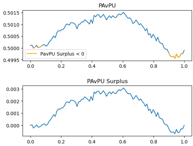
Figure 2: Simulated independent accuracy and uncertainty. PAvPU is meaningless on the orange segment as PAvPU Surplus is smaller than 0

The peak values on the PAvPU curve and the PAvPU Surplus curve have distinct implications. For the PAvPU curve, the peak signifies the optimal uncertainty threshold for distinguishing between accurate and inaccurate predictions. In contrast, the peak of the PAvPU Surplus curve highlights the point at which binary uncertainty yields the greatest insight into accuracy. These peaks might not coincide. For example, with an extremely accurate model, a higher uncertainty threshold might be preferable, even at the cost of making uncertainty information less relevant. This difference is vital for those working on feature engineering, particularly because entropy measures can become very unpredictable without proper thresholding.

7 Dropout as the UQ method and PAvPU Surplus as the UQ metric

In the domain of semantic segmentation, the generation of localized uncertainty estimates plays an indispensable role in assessing the confidence level associated with each pixel-wise prediction, a feature of paramount importance in critical applications like medical imaging and autonomous driving where inaccuracies can lead to dire consequences. The strategic incorporation of dropout within the encoder segments of advanced segmentation networks such as U-Net and Fully Convolutional Networks (FCNs) inherently introduces a degree of variability in the feature representations. This, in turn, subtly influences the decoder’s proficiency in delivering confident predictions, more so in regions characterized by complex semantic content or ambiguous class demarcations. This induced variability echoes the principles of ensemble learning, wherein each forward pass with dropout effectively simulates a distinct "version" of the network, thereby imbuing the model with a multifaceted understanding of its predictions and encapsulating a broader spectrum of epistemic uncertainty, or model uncertainty, which serves as a reflection of the model’s confidence in its learned parameters. [41]

Particularly noteworthy is the impact of this approach on intricate image regions with overlapping objects or nuanced textures, and on the precise delineation of class boundaries, areas where the decoder is challenged by the inconsistent feature sets generated due to encoder dropout. This leads to heightened uncertainty estimates in these critical zones, signifying a cautious stance in the model’s predictions. Such a mechanism is invaluable, for instance, in the realm of medical diagnostics, where an ambiguous area in a tissue scan could necessitate a more conservative interpretation or a second opinion from a medical expert, thus ensuring patient safety [42].

8 Summary

We highlight the necessity of quantifying uncertainty to reveal its underlying assumptions, especially when ground truth uncertainty is unknown. It is possible to put uncertainty quantification into anomaly detection framework, but the task difficulty across models needs to be rebalanced. Furthermore, we do see value in metrics that evaluate both uncertainty and accuracy for a comprehensive assessment, and propose to evaluate models with a metric triplet: (1) accuracy, (2) uncertainty, (3) accuracy & uncertainty. In the following sections, we bring these metrics to the real world.

9 Experimental Analysis

9.1 Objective

As outlined in earlier sections, PAvPU is constrained by its reliance on accuracy and issues stemming from class imbalance. Additionally, the computation of the accuracy value necessitates the grouping of adjacent pixels, making it contingent upon the chosen window size. Therefore, the experiment answers two major questions mentioned in the introduction section: (1) How much does PAvPU depend on accuracy? (2) Is class imbalance an issue for uncertainty quantification? In addition, it answers two minor questions: (1) Is neighboring pixel dependency (window size) an issue? (2) How does PAvPU perform when the patches cross boundaries?

9.2 Computational Environment and Software Stack

2x16 cores IBM POWER9 AC922 CPU, 256 GB RAM, 4 x NVIDIA Volta V100 GPUs, 16GB. mmsegmentation 0.29; Python 3.8; Pytorch 1.9; cuda 12.3.

9.3 Data Description

The Cityscapes Dataset [43] is a large-scale dataset for semantic urban scene understanding, primarily focused on semantic understanding of urban street scenes in the context of autonomous driving and urban scene segmentation. It features high-quality pixel-level annotations of images from 50 different cities, providing a diverse set of visual scenarios. This dataset is widely used in the development and evaluation of machine learning models for tasks such as semantic segmentation, instance segmentation, and panoptic segmentation within urban environments.

9.3.1 Preprocessing Steps

It is common practice to augment the data before feeding them to the model. Data augmentation in image segmentation is a technique used to increase the diversity of training data without actually collecting new images. It helps models to generalize better by exposing them to a wider range of variations within the data, thus improving their performance on unseen images. This is particularly crucial in autonomous driving, where the cost of errors is high and the variety of possible images is vast. In this experiment, we use common techniques to augment Cityscapes Dataset. This includes Random Crop 769 * 769, Horizontal Flip with probability 0.5, Photo Metric Distortion, Random Perturbations of brightness, contrast, saturation and hue and normalization with mean=[123.675, 116.28, 103.53] and std=[58.395, 57.12, 57.375].

9.3.2 Dataset Statistics

Semantic categories in the Cityscapes dataset are divided into several classes that cover a broad range of urban scene components. These categories are grouped into several higher-level categories such as flat, human, vehicle, construction, object, nature, sky, and void. Specifically, the dataset defines 30 classes, out of which 19 are considered for evaluation in segmentation tasks. The training set comprises 2,975 images, while the validation set comprises 500 images. Among all these labels, we emphasize the importance of pedestrians, which unfortunately is not among the majority categories. This raises concerns regarding the imbalance in quantified uncertainty. The major categories encompass roads and buildings, while the minority categories comprise sky, sidewalks, people, riders, walls, cars, fences, trucks, poles, buses, traffic lights, trains, traffic signs, motorcycles, vegetation, bicycles, terrain, and background.

9.4 Methodology

9.4.1 Training Protocol

The introduction of dropout changes the dynamics of the learning process, often necessitating adjustments to other hyperparameters to maintain or improve model performance. [44] Since dropout is essentially training multiple models at the same time, we enlarge the number of iterations to 200k.

9.4.2 Evaluation Framework

Through a traditional interpretation of uncertainty, we restate again the evaluation target of the three metrics: mIoU: accuracy, PAvPU Surplus: uncertainty, PAvPU: joint effect of accuracy and uncertainty. For each model, we run 20 forward loops to get 20 candidate models. The mean level of their uncertainty corresponds to aleatoric uncertainty, whereas their variance represents epistemic uncertainty.

9.4.3 Hyper-paraeter

We use Dropout rate 0.5 for train and validation. Window Size 3, Iterations 200k with SGD optimizer.

10 Experiment Result

10.1 Quantitative Performance

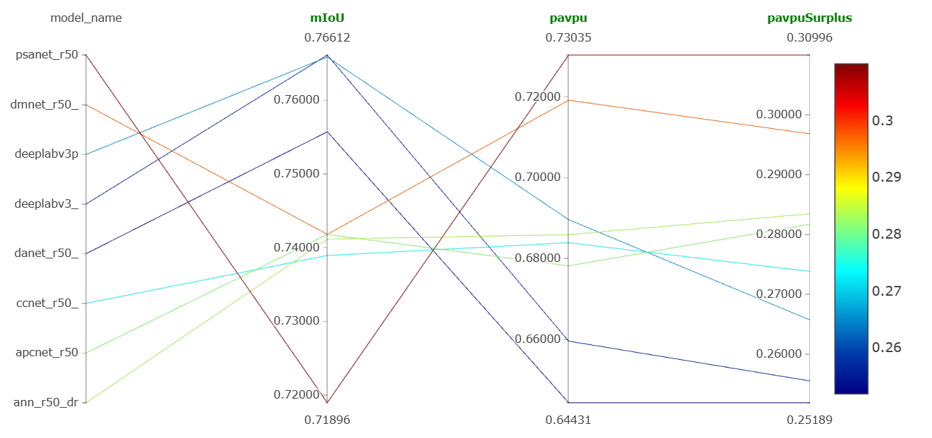
Figure 3: mIoU, PAvPU and PAvPU Surplus indicate different model properties.

Table 1: Benchmark Table for values for Fig. 3

Model	mIoU	PAvPU	PAvPU Surplus
ccnet	0.739	0.684	0.274
ann	0.741	0.686	0.283
apcnet	0.742	0.678	0.282
dmnet	0.742	0.719	0.297
danet	0.756	0.644	0.252
psanet	0.719	0.73	0.31
deeplabv3	0.766	0.66	0.256
deeplabv3+	0.766	0.686	0.264

Figure 3 and Table 1 demonstrate that the three metrics assess models from distinct perspectives, and with no single model outperforming the others across all metrics. Specifically, DeepLabV3+ achieves the highest mean Intersection over Union (mIoU), maintains a relatively high Patch accuracy vs Patch Uncertainty (PAvPU), yet exhibits a diminished PAvPU Surplus, as depicted in Figure 3. We find an interesting result that small models tend to perform better on uncertainty metrics while big models on accuracy metrics. It is possible to ensemble both types to get the benefit of the two. This confirms our proof that PAvPU Surplus complements PAvPU by removing accuracy dependency. We answered question (1). The difference between PAvPU and PAvPU Surplus numerically quantifies accuracy dependency.

Now we seek to numerically answer question (2) the wide class imbalance issue in semantic segmentation. To keep the paper concise, we limit our reporting to two models in Table 5.

We chose these two models due to apcnet’s low mIoU and PAvPU, as well as its high PAvPU Surplus, and conversely deeplabv3 plus’ high mIoU and PAvPU, and low PAvPU Surplus. While deeplabv3 plus is typically regarded as the superior choice, apcnet has demonstrated stronger performance in the critical "Person" category. We restate the importance of reporting the result in categorical levels as the quantified uncertainty differed exponentially across categories. The overall metric does not only neglect but also discriminates against minorities, forcing them to be inaccurate.

Table 2: Categorical PAvPU & PAvPU Surplus across Models

	apcnet		deeplabv3plus
lab	PAvPU	PAvPU+	PAvPU	PAvPU+
0	0,632	0,134	0,670	0,136
1	0,715	0,353	0,719	0,353
2	0,628	0,242	0,626	0,226
3	0,525	0,082	0,577	0,105
4	0,642	0,215	0,728	0,324
5	0,741	0,418	0,723	0,441
6	0,765	0,451	0,727	0,442
7	0,747	0,444	0,725	0,428
8	0,648	0,246	0,590	0,215
9	0,736	0,253	0,740	0,281
10	0,667	0,210	0,553	0,158
11	0,807	0,418	0,785	0,414
12	0,612	0,179	0,677	0,328
13	0,679	0,199	0,704	0,202
14	0,647	0,297	0,716	0,310
15	0,720	0,455	0,823	0,450
16	0,572	0,145	0,743	0,422
17	0,619	0,251	0,671	0,315
18	0,785	0,435	0,743	0,423
mix	0,847	-0,004	0,855	-0,008

The mixed patch refers to the patch that includes multiple categories, found on the edge of an object. As this patch encompasses a wide range of categories, one would expect a minimal connection between precision and uncertainty. In contrast to PAvPU, PAvPU Surplus correctly reflects this. In addition, in scenarios where PAvPU Surplus is negative, the quantified is meaningless and so is the PAvPU. We answered question (4). Due to PAvPU’s accuracy dependency, the meaning of its UQ on the boundary is unclear as accuracy varies across semantic categories. PAvPU Surplus could still provide insights to the trustworthiness of UQ.

Additionally, the investigation included an assessment of window sizes 5 and 7 utilizing the DeepLabV3+ framework to ascertain the reliability of the outcomes with respect to varying window sizes, as the window size is an arbitrary choice. We answered question (3). The findings presented in Table 6 corroborate the consistency of these results.

Table 3: Robestness Test to Window Size

	window size 5		window size 7
lab	PAvPU	PAvPU+	PAvPU	PAvPU+
0	0,680	0,138	0,681	0,137
1	0,739	0,351	0,755	0,354
2	0,643	0,236	0,649	0,232
3	0,592	0,138	0,588	0,114
4	0,735	0,330	0,742	0,324
5	0,759	0,430	0,804	0,445
6	0,762	0,477	0,785	0,468
7	0,751	0,438	0,770	0,420
8	0,604	0,221	0,611	0,218
9	0,751	0,274	0,765	0,282
10	0,568	0,161	0,568	0,153
11	0,815	0,403	0,836	0,394
12	0,697	0,338	0,699	0,318
13	0,720	0,206	0,732	0,203
14	0,719	0,316	0,726	0,308
15	0,833	0,443	0,845	0,464
16	0,739	0,425	0,742	0,407
17	0,668	0,290	0,695	0,323
18	0,771	0,441	0,785	0,436
mix	0,839	0,034	0,805	0,073

10.1.1 Qualitative Insights

We demonstrate another way to visually access model performance without patches.

By using a confusion matrix, we can rule out the badly performed models neglected by PAvPU. Due to the presence of an extra uncertainty output in stochastic models, the confusion matrix gains an extra dimension. We condensed the ground-truth dimension as it is not obtainable and displayed the condensed 3D confusion matrix by a heatmap. The x-axis is the uncertainty percentile, the y-axis is the predicted label. The color indicate the accuracy of pixels fall into the given percentile and predicted label. We demonstrate APCnet in Figure 4 and Deeplabv3 + in Figure 5.

Ideally, the color progression should be consistently darkening from left to right as high uncertainty, if correctly quantified, indicates low accuracy. Based on this standard, it is evident that APCnet outperforms DeeplabV3plus, as shown by the benchmark data for PAvPU Surplus, but not for PAvPU. This phenomenon is attributed to the fact that PAvPU is greatly influenced by the accuracy, where the remarkable accuracy of Deeplabv3+ (as proven by mIoU) compensates for the inadequate estimation of uncertainty.

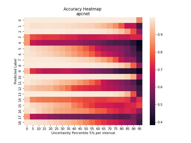
Figure 4: APCnet. The ground truth dimension is collapsed to compute model accuracy.

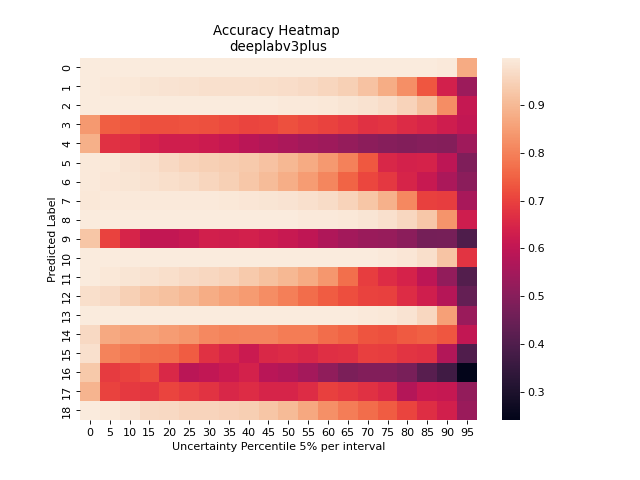
Figure 5: Deeplabv3+. The ground truth dimension is collapsed to compute model accuracy.

11 Conclusion

Initially, we examine three widely recognized metrics for measuring uncertainty and their corresponding methods for uncertainty quantification. We delve into the foundational assumptions of PAvPU, highlighting instances where these might be compromised, such as in cases of imbalanced pixel categories and discrepancies in accuracy. Under these conditions, PAvPU often falls short of its intended purpose. Nonetheless, these challenges are inherent to semantic segmentation models. Through thorough mathematical analysis, we identify the core reasons for these violations. Consequently, we introduce an additional metric, the PAvPU Surplus, to augment PAvPU and ensure its appropriate application.

In our conclusive examination, we assess a set of metrics, including accuracy, PAvPU, and PAvPU Surplus, against the real-world dataset from Cityscapes. This assessment reveals variances among different models, notably in the context of pedestrian categorization, highlighting the need to detail PAvPU and PAvPU Surplus at the category-specific level. In instances involving mixed patches, we observe instances of negative PAvPU Surplus, which emphasizes the critical function of PAvPU Surplus in setting a foundational benchmark for the applicability of PAvPU. Our findings indicate that no single model excels across all three metrics, suggesting the necessity for compromises between models.

For the moment, there is no consensus on the best metrics for quantifying uncertainty, as the preferred choice often varies based on the specific use case (such as the applicable UQ techniques, the requirement to distinguish different types of uncertainty, etc.). PAvPU, being suited for entropy-based uncertainty, presents a significant application. We aim for our detailed review of metrics and the introduction of the auxiliary metric, PAvPU Surplus, to provide direction for the appropriate application of these metrics in semantic segmentation tasks.

12 Appendix

To ease the understanding, we provide without proof the fundamental knowledge on probability.

1) Law of Iterated Expectation: $\mathbf{E}[X]=\mathbf{E}[\mathbf{E}[X|Y]]$

2) Theorem: $\mathbf{E}[g(X)h(Y)|X]=g(X)\mathbf{E}[h(Y)|X]$.

$$PAvPU\_Surplus$$ (3)

$$:=[\mathbf{E}(A_{acc}|U_{cer}=1)-\mathbf{E}(A_{acc})]\mathbf{P}(U_{cer}=1)/\mathbf{std}A_{acc}$$ (4)

$$\text{ }\text{ }\text{ }\text{ }\text{ }+[\mathbf{E}(A_{inacc}|U_{uncer}=1)-\mathbf{E}(A_{inacc})]\mathbf{P}(U_{uncer}=1)/\mathbf{std}A_{inacc}$$ (5)

$$=\mathbf{E}\{U_{cer}[\mathbf{E}(A_{acc}|U_{cer})-\mathbf{E}A_{acc}]\}/\mathbf{std}A_{acc}$$ (6)

$$\text{ }\text{ }\text{ }\text{ }\text{ }+\mathbf{E}\{U_{uncer}[\mathbf{E}(A_{inacc}|U_{uncer})-\mathbf{E}A_{inacc}]\}/\mathbf{std}A_{inacc}$$ (7)

$$=\{\mathbf{E}[\mathbf{E}(U_{cer}A_{acc}|U_{cer})]-\mathbf{E}U_{cer}\mathbf{E}A_{acc}\}/\mathbf{std}A_{acc}$$ (8)

$$\text{ }\text{ }\text{ }\text{ }\text{ }+\{\mathbf{E}[\mathbf{E}(U_{uncer}A_{inacc}|U_{uncer})]-\mathbf{E}U_{uncer}\mathbf{E}A_{inacc}\}/\mathbf{std}A_{inacc}$$ (9)

$$=(\mathbf{E}U_{cer}A_{acc}-\mathbf{E}U_{cer}\mathbf{E}A_{acc})/\mathbf{std}A_{acc}$$ (10)

$$\text{ }\text{ }\text{ }\text{ }\text{ }+(\mathbf{E}U_{uncer}A_{inacc}-\mathbf{E}U_{uncer}\mathbf{E}A_{inacc})/\mathbf{std}A_{inacc}$$ (11)

$$=\mathbf{Cov}(A_{acc},U_{cer})/\mathbf{std}A_{acc}+\mathbf{Cov}(A_{inacc},U_{uncer})/\mathbf{std}A_{inacc}$$ (12)

Note that pixels are by definition either accurate or inaccurate:

$$A_{acc}=1-A_{inacc}$$ (13)

Hence,

$$\mathbf{std}A_{acc}=sqrt[A_{acc}(1-A_{acc})]=sqrt[(1-A_{inacc})A_{inacc}]=\mathbf{std}A_{inacc}$$ (14)

For the same reason:

$$\mathbf{std}U_{cer}=\mathbf{std}U_{uncer}$$ (15)

Also,

$$\mathbf{Cov}(A_{acc},U_{cer})=\mathbf{Cov}(1-A_{acc},1-U_{cer})=\mathbf{Cov}(A_{inacc},U_{uncer})$$ (16)

Therefore,

$$PAvPU\_Surplus=2\times\mathbf{std}(1_{\{U<U_{thres}\}})\mathbf{Corr}(1_{U<U_{thres}},1_{A>A_{thres}})$$ (17)

References

- [1] Spyridon Bakas, Hamed Akbari, Aristeidis Sotiras, Michel Bilello, Martin Rozycki, Justin S Kirby, John B Freymann, Keyvan Farahani, and Christos Davatzikos. Advancing the cancer genome atlas glioma mri collections with expert segmentation labels and radiomic features. Scientific data, 2017.
- [2] Mohammad Havaei, Axel Davy, David Warde-Farley, Antoine Biard, Aaron Courville, Yoshua Bengio, Chris Pal, Pierre-Marc Jodoin, and Hugo Larochelle. Brain tumor segmentation with deep neural networks. Medical Image Analysis, 2017.
- [3] Olaf Ronneberger, Philipp Fischer, and Thomas Brox. U-net: Convolutional networks for biomedical image segmentation. 2015.
- [4] Özgün Çiçek, Ahmed Abdulkadir, Soeren S. Lienkamp, Thomas Brox, and Olaf Ronneberger. 3d u-net: Learning dense volumetric segmentation from sparse annotation. 2016.
- [5] Abhishta Bhandari, Jarrad Koppen, and Marc Agzarian. Convolutional neural networks for brain tumor segmentation. IEEE transactions on medical imaging, 2016.
- [6] Eli Gibson, Francesco Giganti, Yipeng Hu, Ester Bonmati, Steve Bandula, Kurinchi Gurusamy, Brian Davidson, Stephen P. Pereira, Matthew J. Clarkson, and Dean C. Barratt. Automatic multi-organ segmentation on abdominal ct with dense v-networks. IEEE transactions on medical imaging, 2018.
- [7] Holger R. Roth, Le Lu, Amal Farag, Hoo-Chang Shin, Jiamin Liu, Evrim Turkbey, and Ronald M. Summers. Deeporgan: Multi-level deep convolutional networks for automated pancreas segmentation. 2015.
- [8] Özgün Çiçek, Ahmed Abdulkadir, Soeren S. Lienkamp, Thomas Brox, and Olaf Ronneberger. Learning dense volumetric segmentation from sparse annotation. 2016.
- [9] Fang Lu, Fa Wu, Peijun Hu, Zhiyi Peng, and Dexing Kong. Automatic 3d liver location and segmentation via convolutional neural network and graph cut. International Journal of Computer Assisted Radiology and Surgery, 2013.
- [10] Marvin Teichmann, Michael Weber, Marius Zoellner, Roberto Cipolla, and Raquel Urtasun. Multinet: Real-time joint semantic reasoning for autonomous driving. IEEE Intelligent Vehicles Symposium (IV), 2018.
- [11] Xiaozhi Chen, Huimin Ma, Ji Wan, Bo Li, and Tian Xia. Multi-view 3d object detection network for autonomous driving. 2017.
- [12] SBasavaraj Chougula, Arun SADANAND Tigadi, Prabhakar Manage, and Sadanand Kulkarni. Road-segmentation for lidar-based vehicle navigation and autonomous driving. 2019.
- [13] Jinkyu Kim and John Canny. Interpretable learning for self-driving cars by visualizing causal attention. 2017.
- [14] Alex Kendall, Jeffrey Hawke, David Janz, Przemyslaw Mazur, Daniele Reda, John-Mark Allen, Vinh-Dieu Lam, Alex Bewley, and Amar Shah. Learning to drive in a day. 2019.
- [15] Mark Pfeiffer, Michael Schaeuble, Juan Nieto, Roland Siegwart, and Cesar Cadena. From perception to decision: A data-driven approach to end-to-end motion planning for autonomous ground robots. 2018.
- [16] Felipe Codevilla, Matthias Müller, Antonio López, Vladlen Koltun, and Alexey Dosovitskiy. End-to-end driving via conditional imitation learning. 2017.
- [17] Moloud Abdar, Farhad Pourpanah, Sadiq Hussain, Dana Rezazadegan, Li Liu, Mohammad Ghavamzadeh, Paul Fieguth, Xiaochun Cao, Abbas Khosravi, U. Rajendra Acharya, Vladimir Makarenkov, and Saeid Nahavand. A review of uncertainty quantification in deep learning: Techniques, applications and challenges. Information Fusion, page 243–297, 2021.
- [18] Christian Leibig, Vaneeda Allken, Murat Seçkin Ayhan, Philipp Berens, and Siegfried Wahl. Leveraging uncertainty information from deep neural networks for disease detection. Scientific Reports, 2017.
- [19] Christian F. Baumgartner, Kerem C. Tezcan, Krishna Chaitanya, Andreas M. Hötker, Urs J. Muehlematter, Khoschy Schawkat, Anton S. Becker, Olivio Donati, and Ender Konukoglu. Phiseg: Capturing uncertainty in medical image segmentation. 2019.
- [20] Paul K.J. Han, William M.P. Klein, and Neeraj K. Arora. Varieties of uncertainty in health care: a conceptual taxonomy. medical decision making. Medical Decision Making, 2011.
- [21] Amelia Green, William Tillett, Neil McHugh, Theresa Smith, and the PROMPT Study Group. A bayesian network for the assessment and management of musculoskeletal disorders. 2019.
- [22] Michael J. Milford, Janet Wiles, and Gordon F. Wyeth. Solving navigational uncertainty using grid cells on robots. PLOS Computational Biology, 2023.
- [23] Jason Choi, Fernando Castañeda, Claire J. Tomlin, and Koushil Sreenath. Reinforcement learning for safety-critical control under model uncertainty, using control lyapunov functions and control barrier functions. 2020.
- [24] Jishnu Mukhoti and Yarin Gal. Evaluating bayesian deep learning methods for semantic segmentation. https://arxiv.org/abs/1811.12709, 2018.
- [25] Alex Kendall and Yarin Gal. What uncertainties do we need in bayesian deep learning for computer vision? 2017.
- [26] C. E. Shannon. A mathematical theory of communication. Bell System Technical, 1948.
- [27] Chen Liang-Chieh, Papandreou George, Schroff Florian, and Adam Hartwig. Rethinking atrous convolution for semantic image segmentation. In CVPR, 2017.
- [28] Liang-Chieh Chen, Yukun Zhu, George Papandreou, Florian Schroff, and Hartwig Adam. Encoder-decoder with atrous separable convolution for semantic image segmentation. In ECCV, 2018.
- [29] Huang Zilong, Wang Xinggang, Huang Lichao, Huang Chang, Wei Yunchao, and Liu Wenyu. Ccnet: Criss-cross attention for semantic segmentation. In ICCV, 2019.
- [30] Zhu Zhen, Xu Mengde, Bai Song, Huang Tengteng, and Bai Xiang. Asymmetric non-local neural networks for semantic segmentation. In ICCV, 2019.
- [31] He Junjun, Deng Zhongying, Zhou Lei, Wang Yali, and Qiao Yu. Adaptive pyramid context network for semantic segmentation. In CVPR, 2019.
- [32] He Junjun, Deng Zhongying, and Qiao Yu. Dynamic multi-scale filters for semantic segmentation. In ICCV, 2019.
- [33] Jun Fu, Jing Liu, Haijie Tian, Yong Li, Yongjun Bao, Zhiwei Fang, and Hanqing Lu. Dual attention network for scene segmentation. In CVPR, 2019.
- [34] Zhao Hengshuang, Zhang Yi, Liu Shu, Shi Jianping, Change Loy Chen, Lin Dahua, and Jia Jiaya. Psanet: Point-wise spatial attention network for scene parsing. In ECCV, 2018.
- [35] Chuan Guo, Geoff Pleiss, Yu Sun, and Kilian Q. Weinberger. On calibration of modern neural networks. 2017.
- [36] Fredrik K. Gustafsson, Martin Danelljan, and Thomas B. Schön. Evaluating scalable bayesian deep learning methods for robust computer vision. 2020.
- [37] Yanwu Yang, Xutao Guo, Yiwei Pan, Pengcheng Shi, Haiyan Lv, and Ting Ma. Uncertainty quantification in medical image segmentation with multi-decoder u-net. 2021.
- [38] Ling Huang, Su Ruan, Pierre Decazes, and Thierry Denœux. Deep evidential fusion with uncertainty quantification and contextual discounting for multimodal medical image segmentation. arXiv:2309.05919, 2023.
- [39] Eyke Hüllermeier and Willem Waegeman. Aleatoric and epistemic uncertainty in machine learning: an introduction to concepts and methods. Machine Learning, page 457–506, 2021.
- [40] Pearson Karl. On the theory of contingency and its relation to association and normal correlation. 1904.
- [41] Yarin Gal and Zoubin Ghahramani. Dropout as a bayesian approximation: Representing model uncertainty in deep learning. 2016.
- [42] Sivaramakrishnan Rajaraman, Ghada Zamzmi, Feng Yang, Zhiyun Xue, Stefan Jaeger, and andSameer K. Antani. Uncertainty quantification in segmenting tuberculosis-consistent findings in frontal chest x-rays. Biomedicines, 2022.
- [43] Marius Cordts. The cityscapes dataset for semantic urban scene understanding. CVPR, 2016.
- [44] Nitish Srivastava. Dropout: A simple way to prevent neural networks from overfitting. Journal of Machine Learning Research, 2023.