Performance Evaluation of IEEE 802.11bf Protocol in the sub-7 GHz Band

Abstract

Changes in Wi-Fi signal, using Wi-Fi sensing, have been used to detect movements in the environment and have led to development of many related applications. However, there has not been a standard way to do this until the IEEE 802.11bf standard development activity was taken up recently by the IEEE. Wi-Fi sensing is an overhead to data communication. While the IEEE 802.11bf standard has been designed with careful attention to the overhead and its impact on data communication, there has been no study done to quantify those. Therefore, in this paper, we evaluate performance of IEEE 802.11bf protocol with different system configurations corresponding to different sensing loads and the impact of sensing on data communication in those configurations. We outline some of the key findings from our simulation experiments which may be useful in practical operating configurations of an IEEE 802.11bf network.

I Introduction

Using Wi-Fi sensing, changes in Wi-Fi radio channel can be used to detect movements in the environment enabling a wide range of applications such as presence of humans, localization, fall detection etc. [1]. Since Wi-Fi networks are widely deployed, the above paradigm would make it possible to make aforementioned diverse set of applications available to the users and eliminate the need for different kind of sensors for different applications. Although a lot of work has been reported in the literature about Wi-Fi based sensing  [1, 2, 3, 4, 5, 6, 7, 8], lack of standardization has limited the proliferation of Wi-Fi sensing based applications. Therefore, the Task Group IEEE 802.11bf (TGbf) started the development of an amendment to the IEEE 802.11 standard in September 2020 to standardize Wi-Fi based sensing [9] which will be known as IEEE 802.11bf. The IEEE 802.11bf standard defines Wireless Local Area Network (WLAN) sensing procedures, both in the sub-7 GHz [9, 10] and above 45 GHz band [9, 11].

Integrating sensing with data communication in Wi-Fi network is quite attractive since it allows for more efficient use of spectrum and hardware. However, for sensing, the system may need to allocate a part of its radio resources to send dedicated sounding frames and other sensing related information, reducing resources available for regular data communication. Thus, sensing may become an overhead for data communication. Hence, TGbf has given careful attention to the design of WLAN sensing procedure to limit the sensing overhead and its impact on communication performance. But, to the best of our knowledge, there is no performance study available to quantify the sensing performance and the impact of sensing on communication. Therefore, in this paper, we evaluate WLAN sensing performance and the impact of WLAN sensing on communication using performance metrics defined by us.

In the IEEE 802.11bf sensing protocol for sub-7 GHz, the actual sensing measurements are done during, what are called, sensing measurement exchanges (SMEs) and those SMEs account for most of the sensing overhead. So, in this performance study, we focus on the SME part of the protocol. To perform an SME, the initiator of sensing, which could be the Access Point (AP) or a Wi-Fi Station (STA), has to get access to the channel and obtain a Transmission Opportunity (TxOP). It may use Enhanced Distributed Channel Access (EDCA) or Point coordination function (PCF) Interframe Space (PIFS) to get a TxOP. The IEEE 802.11bf protocol also defines a periodically occurring sensing window within which the SMEs have to be performed. The duration and periods of sensing windows are configurable. Our simulation based performance study examines both the EDCA and PIFS based access methods at different sensing load in the system when the AP is the initiator of sensing. The sensing load in the system is varied by varying the number of sensing STAs, the number of sensing applications, the number of transmit and receive antennae and the sensing window duration. We present an extensive set of simulation results at different system configurations corresponding to different sensing loads. We then highlight some important and interesting findings from our simulation results which, we believe would be useful in configuring IEEE 802.11bf systems in the sub-7 GHz band.

The main contributions of this work are as follows.

• To the best of our knowledge, this is the first work to present extensive simulation of the IEEE 802.11bf protocol.

• This work provides quantitative insights into performance of the IEEE 802.11bf protocol in terms of defined performance metrics.

• Our simulation exposes limitations of WLAN sensing using EDCA based access when sensing reports need to be sent from sensing STAs to the AP.

• The results presented in this work provide guidance and insights into practical operating configurations of an IEEE 802.11bf network.

II Related Work

There has been a lot of research work on Wi-Fi reported in the literature. In [3], the authors present a passive Wi-Fi radar system for human sensing by exploiting high data rate OFDM signals and periodic Wi-Fi beacon signals. Change in Received Signal Strength (RSS) in a commercial off-the-shelf (COTS) Wi-Fi device held on a person’s chest is used to design a respiratory monitoring system in [2]. Changes in Wi-Fi signal strength have been studied to detect hand gestures around a user’s mobile device in [4]. In [6], the authors have implemented an end-to-end system to monitor human respiratory motion using Wi-FI Channel State Information (CSI). They propose a deep learning based processing algorithm called BreatheSmart that anaylzes the changes in amplitude and phase of CSI data to detect respiratory motion. In [7], a four antenna passive bistatic indoor radar configuration is set up using IEEE 802.11ax Wi-Fi system to track multi-target human based on range, doppler and angle-of-arrival measurements. A prototype of Wi-Fi based passive radar system for localization and tracking of moving targets using range, doppler and direction of arrival is presented in [8]. The above mentioned research works are focused on methodologies or algorithms for the concerned applications, but do not deal with estimating the Wi-Fi sensing related overhead of the system. A fairly comprehensive survey of Wi-Fi sensing with CSI is presented in [1].

To standardize Wi-Fi sensing process, the TGbf is developing a standard which will be known as IEEE 802.11bf [9]. This standard defines the mechanisms and protocols to provide channel state information in the sub-7 GHz band and radar based information (e.g., range, doppler, beam azimuth) above 45 GHz band. Since Wi-Fi sensing protocol is an overhead to the Wi-Fi data communication, it is important to study the performance of Wi-Fi sensing and its impact on data communication in different configurations. To the best of our knowledge, there is no such study available in the literature. This paper is the first to report performance analysis of IEEE 802.11bf protocol in various configurations.

III Overview of IEEE 802.11bf Sensing Procedure

An IEEE 802.11bf capable STA and AP exchange their sensing capabilities during the association process. WLAN sensing in the sub-7 GHz band, referred to as Sensing Procedure, starts out with the establishment of a sensing measurement session between a sensing initiator and a sensing responder at which time the operating parameters of the session are determined. Examples of operating parameters include bandwidth, role of the STAs (sensing transmitter or sensing receiver), timer values etc. The actual sensing measurements are performed in SMEs. SMEs can be trigger based (TB) or non-trigger based (NTB). Since TB SME is envisioned to be the most common deployment scenario, in this study, we focus on TB SME. In a TB SME an AP is the sensing initiator and one or more non-AP STAs are the sensing responders. A TB SME can have up to four phases as shown in Fig. 1. In the polling phase, an AP (the sensing initiator) sends a Sensing Polling Trigger frame to the sensing responder STAs to participate in the SME during a sensing availability window (SAW). A SAW has two parameters: SAW duration and SAW period. SAW durations occur periodically and the period is determined by SAW period. An AP and the STAs may participate in SMEs only in a SAW duration. In the Null Data Packet Announcement (NDPA) Sounding phase the AP is the sensing transmitter and one or more STAs are the sensing receivers. The AP sends a NDPA frame followed by a Null Data Packet (NDP) frame to the receiver STAs. The STAs measure the channel state using the received NDP frame. In the Trigger Frame (TF) Sounding phase, the AP acts as the sensing receiver and the STAs as sensing transmitters. The AP sends a TF to the sensing receiver STAs, which then send NDP frames (which are multiplexed in the spatial domain) to the AP. The AP measures the channel state using the received NDP frames. Reporting phase is present, if sensing report (mainly consisting of CSI) is required to be sent from the STAs to the AP. Orthogonal Frequency Division Multiple Access (OFDMA) mechanism is used for reporting, for which the AP allocates Resource Units (RUs) to the STAs. Only NDPA sounding phase may necessitate a Reporting phase, if reporting was enabled as part of operational parameters during sensing measurement session set up. For more details on TB SME, please refer to [9].

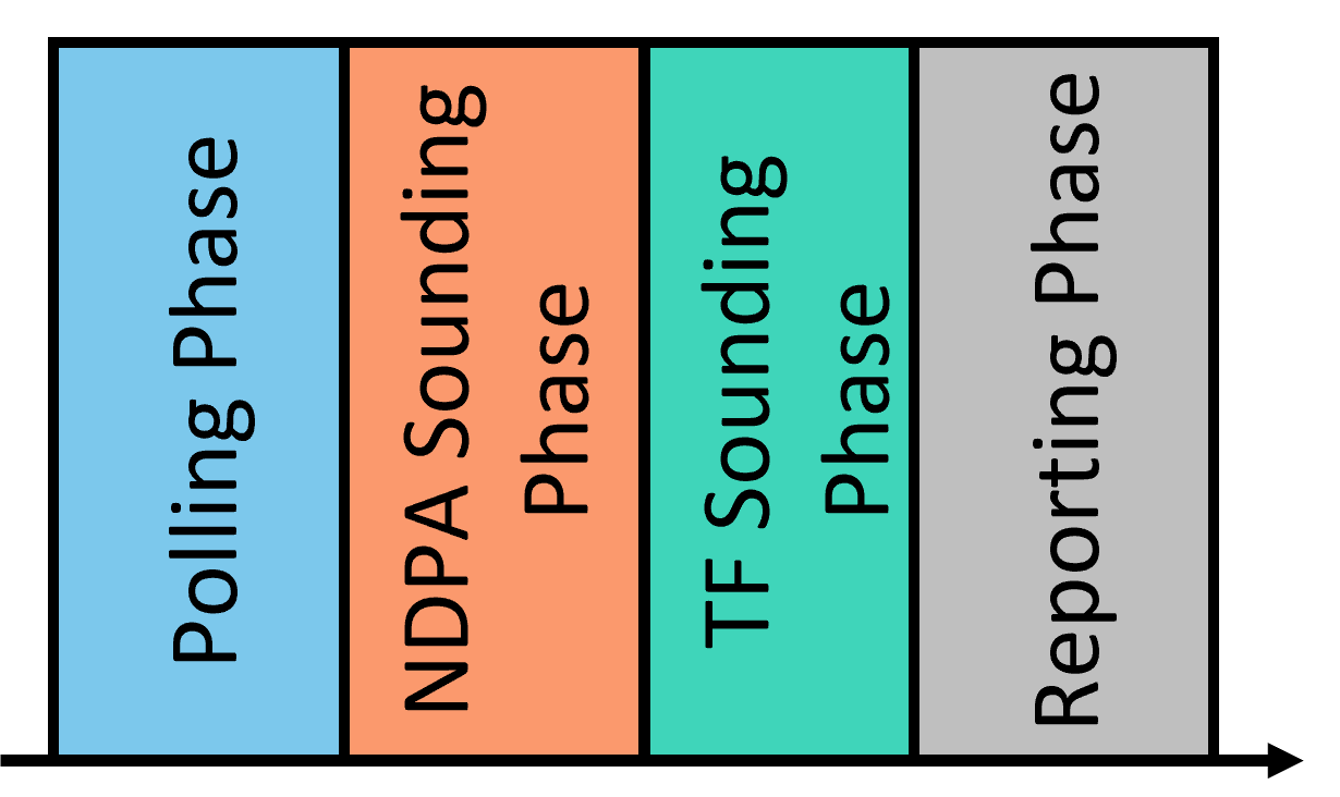
Figure 1: Different phases in a TB Sensing Measurement Exchange

An AP starts an SME by obtaining a TxOP after a SAW period starts. It may obtain the TxOP by EDCA or PIFS mechanism. We refer to them as EDCA access and PIFS access respectively. If it uses EDCA access, then due to contention, the actual SAW duration available for SME sometimes may be shorter than the configured SAW duration. But when PIFS access is used, AP gets priority access to the channel and hence, gets almost the entire SAW duration for sensing.

III-A Overhead Calculation

The Sensing Procedure is an overhead for data communication. Majority of the overhead is incurred in the SME part of the protocol. So, in this study, we concentrate on the SME of the protocol. In an SME, the NDPA sounding phase and Reporting phase account for most of the overhead. Hence, our overhead calculation involves only those two phases. Note that in an NDPA sounding phase, the AP acts as a sensing transmitter and one or more STAs act as sensing receivers. For the NDPA sounding phase, we take the number of bytes in NDPA and NDP frame structure as overhead [9]. The NDPA frame structure is presented in Fig. 9.58 in [12] and the STA Info field format used in NDPA frame is shown in Fig. 9-61da in [13]. The NDP format shown in Fig. 27.46a in [13] is used for computation of NDP overhead. For the reporting overhead, we use the CSI size computation used in Equation (9-5f) in [9]:

$$\begin{split}CSI\,size=&\lceil 1.5\times N_{tx}\times N_{rx}\rceil+\frac{N_{tx}\times N_{rx}\times N_{b}\times N_{sc}}{4}\\ &+2\times N_{rx},\end{split}$$ (1)

where $N_{tx}$ is the number of transmit antennas, $N_{rx}$ is the number of receive antennas, $N_{b}$ is the number of bits used for quantization of each CSI value, $N_{sc}$ is the number of subcarriers reported in CSI. The bytes transmitted as part of NDPA, NDP, and reporting frame will be referred to by a general term called sensing information bytes throughout this paper.

IV Simulation Experiments

IV-A Simulation Setup

In our simulation setup, in terms of network topology, we assume that there is one AP and a variable number of STAs associated with the AP. Our simulation assumes that all messages are received correctly by the receiver, i.e., there is no message error due to interference.

We assume that each sensing application runs on every STA in the network and that the AP requires CSI report from every STA in the network for a given sensing application. Due to resource limitation, if a complete report cannot be sent from a STA, the STA still sends a partial report. Although in practice, this will not happen, we resort to this method to highlight the sensing overhead and the missed sensing that such cases lead to. When there is no sensing activity in the network, the STAs send data traffic using EDCA with full bandwidth. We assume that each STA always has at least a TxOP worth of data to be sent. The TxOP duration was set to its maximum value of 5.484 ms [14]. The AP only participates in sensing and does not send any data traffic.

Performance evaluation of systems at high load is usually more interesting. Since the SME part of the Sensing Procedure incurs most of the overhead, it leads to high sensing load. Hence, it is the focus of our simulation. As mentioned in Section III-A, we compute overhead based on the NDPA sounding and Reporting phase of an SME. During Reporting phase, the AP allocates one RU (RU sizes given in Table II) to each STA which is used by each STA to send sensing reports using OFDMA. We have implemented our simulation code by incorporating IEEE 802.11bf features into the software available at [15], which was used in the simulation study reported in [14].

IV-B Performance Metrics

We define the following performance metrics in our evaluation.

• Percentage Sensing Overhead (PSO): It is the percentage of total simulation duration spent on exchanging sensing related messages.

• Percentage Sensing Missed (PSM): In every SAW period, sensing is considered to be complete, if all the sensing messages, for all the applications, were able to be sent in the SAW duration. If no sensing messages were sent (completely missed) or only a part of sensing messages were sent (partially missed), then we consider those cases as sensing missed. So, the percentage of the number of SAW periods in which sensing is missed is defined as Percentage Sensing Missed (PSM).

• Data Throughput: This is the total number of data bits sent by all the STAs divided by the simulation time.

• Percent Available Window Duration (PAWD): This is defined as the percentage of SAW duration actually available for sensing related tasks. Note that when EDCA acess is used, some part of SAW duration may be lost due to contention. In such situations, the PAWD would fall below 100 %.

TABLE I: Simulation Parameters Common to all Configurations

Parameter	Value
Sensing availability window period	1 (=100 TU = 102.4 ms)
TxOP duration	5.484 ms
Number of antennas in the AP	8
Number of antennas in each STA	2
AP Bandwidth	80 MHz
STA Bandwidth	80 MHz
maximum number of subcarriers	996
subcarrier grouping ($N_{g}$)	4
Number of subcarriers reported in CSI ($N_{sc}$)	250
Number of bits used for quantization of each CSI value ($N_{b}$)	8
EDCA transmission in a TxOP	Payload = 10 ethernet packets of size 1500 bytes each in an A-MPDU
MCS	6
Simulation duration	10000 seconds

TABLE II: Subcarrier Allocation vs. Number of STAs

Number of STA	Subcarriers per STA (size of RU allocation per STA)
1	996
2	484
[3 - 4]	242
[5 - 9]	106
[10 - 16]	52

IV-C Simulation Experiment Design

Three parameters decide the sensing load in an IEEE 802.11bf network: (i) number of sensing STAs, (ii) number of sensing applications, and (iii) number of transmit and receive antennae involved in sensing. Hence, for this performance study, we increased the sensing load in the system by increasing the value of one of those parameters while keeping the values of other two constant. This led us to run our experiments in three configurations as described below.

• Configuration 1: In this configuration, sensing load is increased by increasing the number of STAs (nSTAs) involved in sensing at different SAW durations. The number of applications is fixed at 4 and the sensing transmitter and receiver antenna configuration is set to 2x2. Note that sensing transmitter and receiver antenna configuration 2x2 implies that for each STA, the AP (sensing transmitter) uses two of its eight antenna and each STA (sensing receiver) uses all of its two antenna. Thus, the AP can engage with up to four STAs in an SME for sensing.

• Configuration 2: Sensing load, in this configuration, is increased by increasing the number of sensing applications (numapp) in the system at different nSTA values. The SAW duration is fixed at 127 (Note: SAW duration 1 = 100 $\mu$s), which corresponds to its maximum possible value of 12.7 ms. The sensing transmitter and receiver antenna configuration is set to 2x2.

• Configuration 3: Sensing load is increased by involving more transmit and receive antennae, referred to as sensing transmitter and receiver antenna (STRA) configuration, at different nSTA values. The number of application is fixed at 4 and SAW duration is fixed at 127 (12.7 ms).

Simulation parameters common to all configurations are shown in Table I.

IV-D Experiment Results

IV-D1 Configuration 1

Fig. LABEL:fig:edca_nsta_pso shows how PSO changes as nSTA increases with EDCA access. Generally, PSO decreases as nSTA increases, because there is more contention for getting TxOP for sensing and hence, less duration is available for sensing. However, PSO increases from nSTA = 4 to 5 and from nSTA = 9 to 10 for SAW duration $>$ 10. At these nSTA transition points the size of an RU assigned to each STA goes down (see Table II), hence, more time is needed to send a given number sensing information bytes thereby increasing the overhead. SAW duration 10 (1 ms) is very short relative to the SAW period of 102.4 ms. Hence, the overhead is very low in this case and at high nSTA, due to high contention, PSO goes down to almost zero.

As seen in Fig. LABEL:fig:pifs_nsta_pso, with PIFS access, PSO remains unchanged when RU size per STA does not change. Unlike EDCA access, there is no variability in actual SAW duration available for sensing since no contention is involved. Report size per STA does not change since the number of application is constant in this configuration. Hence, PSO remains constant in the intervals where RU size per STA does not change. But when RU size per STA decreases (e.g., from nSTA = 9 to 10), the duration to send sensing report goes up and hence, PSO goes up. SAW duration = 10 is too short which limits the number of sensing information bytes sent, to a constant value across the nSTA values and hence, PSO does not change. Note that PSO for SAW duration 90 and 127 are identical all throughout. For these two SAW durations PSM is 0 % all throughout (see Fig. LABEL:fig:pifs_nsta_psm). Hence, the amount of sensing information bytes sent is same for the two SAW durations. For SAW duration 50, PSO is identical to those of SAW duration 90 and 127 until nSTA=9, since PSM is 0 % until that point. But after that PSM goes up to 100 %. But these missed sensing are due to partial missed sensing and PSO beyond nSTA=9 is just 0.04 % lower than those of SAW durations 90 and 127. Hence, its PSO looks almost identical to them after nSTA=9. This indicates that SAW duration 50 fell slightly short of the duration needed to send all the sensing information bytes.

With EDCA access, as nSTA increases, PSM increases (see Fig. LABEL:fig:edca_nsta_psm). Due to more contention, actual SAW duration available for sensing decreases, hence, more sensing is missed. SAW duration 10 is too short for EDCA such that $100\,\%$ sensing is always missed. Except for nSTA = 1 none of the configurations can give $0\,\%$ PSM, which is important for sensing application performance. For SAW duration = 10, even though PSM is $100\,\%$, there is overhead which is due to partial missed sensing.

SAW duration 10 is too short even for PIFS access, hence $100\,\%$ sensing is missed (see Fig. LABEL:fig:pifs_nsta_psm). But SAW duration 90 and 127 give $0\,\%$ throughout. SAW duration 50 is not long enough, beyond nSTA = 9, to send all the sensing information bytes, due to decrease in RU size per STA.

With EDCA access, from Fig. LABEL:fig:edca_nsta_thrpt, it can be seen that throughput goes down when sensing is on (compared to no sensing). As nSTA increases, throughput decreases due to more contention and collisions. Also, as SAW duration increases, throughput decreases because more time is used for sensing. For SAW duration 10 and nSTA $\geq$ 3, throughput almost equals to that of no sensing case because actual available sensing duration becomes very short due to higher TxOP contention.

As shown in Fig. LABEL:fig:pifs_nsta_thrpt, with PIFS access, throughput is lower than the respective EDCA cases due to higher sensing overhead (and lower missed sensing). The throughput of SAW duration 50, 90 and 127 are almost equal since sensing overheads for these cases are almost equal.

With EDCA access, PAWD generally decreases as nSTA increases due to increase in contention (see Fig. LABEL:fig:config1_pawd). As expected, higher the SAW duration, higher is the PAWD. PAWD is found to be always $100\,\%$ or very close to $100\,\%$ for PIFS access (not shown in a graph).

IV-D2 Configuration 2

With EDCA access, PSO generally increases as numapp increases (Fig. LABEL:fig:edca_numapp_pso). At high numapp (e.g., 6 and 8), for nSTA = 12 and nSTA = 16, PSO remains flat, because the number sensing report bytes that can be sent in the SAW duration is limited by the RU size allocated to the STA. This can also be explained through PSM graph in Fig. LABEL:fig:edca_numapp_psm where between numapp = 6 and 8, PSM becomes $100\,\%$ for nSTA = 12 and 16. We notice that the overhead of nSTA = 12 is more than nSTA=16 which is counter intuitive. With nSTA = 16, there is less duration available for sensing due to more contention. Hence, nSTA = 12 gets more sensing opportunities and incurs higher overhead. We also notice that for nSTA = 8, overhead goes beyond nSTA = 12 and 16 at numapp = 8. nSTA = 8 has larger RU size than nSTA = 12 and 16 and hence, could send more sensing information bytes than nSTA = 12 and 16.

In case of PIFS access, overhead consistently increases as numapp increases and nSTA increases (see Fig. LABEL:fig:pifs_numapp_pso). This can be explained by observing PSM (see Fig. LABEL:fig:pifs_numapp_psm), where there is no sensing missed. Hence overhead increases with increase in numapp and also with increase in nSTA.

Fig. LABEL:fig:edca_numapp_psm shows that with EDCA access, as numapp increases, PSM increases. At some nSTA values, the jump is more drastic at certain numapp. For example, For nSTA = 12 and 16, as numapp increase from 4 to 6, the report size increases such that with the allocated RUs full report cannot be sent even for one application. Hence, PSM increases drastically to $100\,\%$. For nSTA = 1 and 4, the numapp increase does not affect PSM due to low report size.

In case of PIFS access (see Fig. LABEL:fig:pifs_numapp_psm), there is no missed sensing in any configuration since PIFS gives priority access to the channel and the SAW duration 127 is long enough to send all sensing information bytes.

With EDCA access (see Fig. LABEL:fig:edca_numapp_thrpt), for a given nSTA, the throughput goes down slowly as numapp increases since it is only affected by the report size increase. But for a given numapp, as nSTA increases throughput drops much more due to higher contention and collisions as well as due to report size increase. For nSTA = 12 and 16, as numapp increases from 6 to 8, throughput remains flat because the PSO in this case does not change (see Fig. LABEL:fig:edca_numapp_pso).

From Fig. LABEL:fig:pifs_numapp_thrpt, we observe that with PIFS access, throughput decrease is steeper than EDCA access as numapp increases, since PIFS access incurs $0\,\%$ PSM and higher sensing overhead than EDCA access.

Fig. LABEL:fig:config2_pawd shows the PAWD performance for EDCA access. Since SAW duration is 12.7 ms and TxOP is 5.484 ms, sensing can have up to three TxOPs. When nSTA is small (1 and 4), then increasing numapp does not change the duration and the number of TxOPs required to complete sensing. Hence, PAWD remains almost constant. But at large nSTA and large numapp, (e.g., nSTA = 12 and numapp = 6), it requires more TxOPs to finish sensing operation. Since each TxOP is subject to contention, PAWD comes down. PAWD is always $100\,\%$ or close to $100\,\%$ for PIFS access (not shown).

IV-D3 Configuration 3

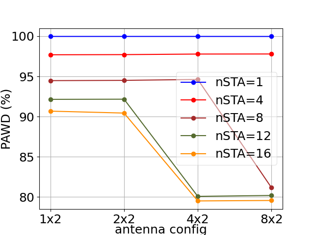
Figure 3: Available Window Duration vs. number of STAs with EDCA Access (Configuration 3)

With EDCA access, as STRA increases, PSO generally increases (see Fig. LABEL:fig:edca_antenna_pso). For nSTA = 12 and 16 PSO remains flat from STRA = 4x2 to 8x2, because the number of sensing information bytes that can be sent in the SAW duration is limited by the RUs assigned to the STAs. This is similar to what was seen in Configuration 2. Between nSTA = 12 and 16, the overhead of nSTA = 12 is more than nSTA = 16, which is again similar to Configuraiton 2 and the same explanation is applicable. We also notice that for nSTA = 8, overhead goes beyond nSTA = 12 and 16 at STRA 8x2. nSTA = 8 has larger RU size than nSTA = 12 and 16. Hence, nSTA = 8 could send more sensing information bytes than nSTA = 12 and 16 which results in higher PSO.

With PIFS access, as shown in Fig. LABEL:fig:pifs_antenna_pso, PSO goes up as STRA increases. As STRA increases report size also increases which leads to more overhead. Overhead for nSTA = 12 and 16 are the same throughout, since RU size per STA and PSM are same for them.

With EDCA access, as STRA increases, generally PSM also increases (see Fig. LABEL:fig:edca_antenna_psm). Since nSTA = 8 has larger RU size, it does not hit $100\,\%$ until STRA = 8x2. nSTA = 12 and 16 have smaller RU size, hence they hit $100\,\%$ at a lower STRA = 4x2. For a given STRA configuration, as nSTA increases, more sensing is missed due to the larger report size and more contention to claim TxOP.

For PIFS access, as shown in Fig. LABEL:fig:pifs_antenna_psm, PSM is mostly $0\,\%$, except for STRA = 8x2 and nSTA = 12 and 16 when the report size becomes too large for the RUs assigned to the STAs and PSM hits $100\,\%$.

From Fig. LABEL:fig:edca_antenna_thrpt, for EDCA access we notice that generally throughput decreases as STRA configuration increases due to increase in sensing overhead. Also as nSTA increases for a given STRA configuration, throughput decreases due to more contention as well as due to higher sensing overhead. For nSTA = 12 and nSTA = 16 between STRA = 4x2 and 8x2, throughput is flat because the corresponding PSO is also flat.

In Fig. LABEL:fig:pifs_antenna_thrpt it is observed that, with PIFS access, throughput drops more than EDCA access case as STRA configuration increases because of more sensing overhead. Between STRA = 4x2 and 8x2 throughput drop is more drastic which matches with corresponding drastic increase in sensing overhead.

PAWD performance with EDCA access, shown in Fig. 3, is very similar to the that in Configuration 2. Hence, the same explanation holds. For PIFS access PAWD is always 100 % or close to 100 %.

IV-D4 Discussion

From the above discussions on our simulation results, we highlight the following key points. Since keeping PSM to $0\,\%$ is important for the performance of a sensing application, EDCA access is not a suitable option as it can lead to missed sensing in almost all cases. So, PIFS based access should be used for sensing. Very short PAW duration (e.g., 10) is not a good choice even at very low sensing load since it leads to missed sensing. In fact, with PIFS access, it is better to set the SAW duration to its maximum value 127 to avoid missed sensing, since the performance impact of sensing on data communication in terms of PSO and throughput is almost identical to smaller SAW durations at which there is no missed sensing. With PIFS access, when numapp = 4 and nSTA = 16, the overhead is about $5\,\%$ and the throughput drops by about 8 Mbps (or about $5\,\%$) compared to “no sensing” case. Considering that this is a very high sensing load situation, the overhead and throughput drop may be acceptable. Another important thing to note is that the RU size changes at discrete points (with respect to nSTA) and there can be sudden change of performance or performance may seem counter-intuitive at those change points. These results also show that a system can be designed with an upper limit on sensing overhead. The AP in such a system would allow the sensing load to increase (by having more applications, stations or more antennae), until the sensing overhead limit is reached.

V Conclusion

IEEE 802.11bf is a relatively new standard for Wi-Fi sensing. While integrating sensing with communication in Wi-Fi network leads to more efficient use of spectrum and hardware, it also contributes to communication overhead. Although the TGbf has carefully designed the IEEE 802.11bf protocol to limit the overhead, there is no performance analysis of the protocol and its impact on data communication available in the literature. In this paper, we evaluate performance of the protocol and its impact on data communication using performance metrics defined by us. Our simulation results show that, when NDPA sounding phase with reporting is enabled, EDCA access is not suitable for sensing since it can lead to missed sensing. Also, very short SAW duration (e.g., 10), even at low sensing load, is not a good choice since it leads to missed sensing. A good rule of thumb is to have PIFS access with SAW duration set to a large value (e.g., its maximum value of 127), which ensures $0\,\%$ PSO in almost all the cases.

References

- [1] Y. Ma, G. Zhou, and S. Wang, “WiFi sensing with channel state information: A survey,” ACM Computing Surveys (CSUR), vol. 52, no. 3, pp. 1–36, 2019.
- [2] H. Abdelnasser, K. A. Harras, and M. Youssef, “Ubibreathe: A ubiquitous non-invasive wifi-based breathing estimator,” in Proceedings of the 16th ACM international symposium on mobile ad hoc networking and computing, 2015, pp. 277–286.
- [3] W. Li, R. J. Piechocki, K. Woodbridge, C. Tang, and K. Chetty, “Passive wifi radar for human sensing using a stand-alone access point,” IEEE Transactions on Geoscience and Remote Sensing, vol. 59, no. 3, pp. 1986–1998, 2020.
- [4] H. Abdelnasser, M. Youssef, and K. A. Harras, “Wigest: A ubiquitous wifi-based gesture recognition system,” in 2015 IEEE conference on computer communications (INFOCOM). IEEE, 2015, pp. 1472–1480.
- [5] S. Arshad, C. Feng, Y. Liu, Y. Hu, R. Yu, S. Zhou, and H. Li, “Wi-chase: A wifi based human activity recognition system for sensorless environments,” in 2017 IEEE 18th International Symposium on A World of Wireless, Mobile and Multimedia Networks (WoWMoM). IEEE, 2017, pp. 1–6.
- [6] S. Mosleh, J. B. Coder, C. G. Scully, K. Forsyth, and M. O. A. Kalaa, “Monitoring respiratory motion with Wi-Fi CSI: Characterizing performance and the BreatheSmart algorithm,” IEEE Access, pp. 1–1, 2022.
- [7] L. Storrer, H. C. Yildirim, M. Crauwels, E. I. P. Copa, S. Pollin, J. Louveaux, P. De Doncker, and F. Horlin, “Indoor tracking of multiple individuals with an 802.11ax Wi-Fi-based multi-antenna passive radar,” IEEE Sensors Journal, vol. 21, no. 18, pp. 20 462–20 474, 2021.
- [8] P. Falcone, F. Colone, A. Macera, and P. Lombardo, “Localization and tracking of moving targets with WiFi-based passive radar,” in 2012 IEEE Radar Conference, 2012, pp. 0705–0709.
- [9] “IEEE p802.11bf™/d3.0 draft standard for information technology— telecommunications and information exchange between systems local and metropolitan area networks— specific requirements part 11: Wireless LAN medium access control (MAC) and physical layer (PHY) specifications amendment 2: Enhancements for wireless LAN sensing,” 2023.
- [10] T. Ropitault, S. Blandino, A. Sahoo, and N. Golmie, “IEEE 802.11bf: Enabling the widespread adoption of wi-fi sensing,” accepted in IEEE Communications Standards Magazine: https://tsapps.nist.gov/publication/get_pdf.cfm?pub_id=935175, [Online; accessed September 28, 2023].
- [11] S. Blandino, T. Ropitault, C. R. da Silva, A. Sahoo, and N. Golmie, “IEEE 802.11 bf DMG sensing: Enabling high-resolution mmwave wi-fi sensing,” IEEE Open Journal of Vehicular Technology, vol. 4, pp. 342–355, 2023.
- [12] “Part 11: Wireless LAN Medium Access Control (MAC) and Physical Layer (PHY) Specifications,” 802.11 Working Group of the LAN/MAN Standards Committee of the IEEE Computer Society, Dec. 2020.
- [13] “IEEE p802.11az™/d7.0 draft standard for information technology— telecommunications and information exchange between systems local and metropolitan area networks— specific requirements part 11: Wireless LAN medium access control (MAC) and physical layer (PHY) specifications amendment 4: Enhancements for positioning sensing,” 2022.
- [14] Y. Daldoul, D.-E. Meddour, and A. Ksentini, “Performance evaluation of ofdma and mu-mimo in 802.11 ax networks,” Computer Networks, vol. 182, p. 107477, 2020.
- [15] “802.11ax lightsim,” https://github.com/yousri-daldoul/802.11ax-lightsim, accessed April 2023.